Article

Shape Adaptive Neighborhood Information-Based Semi-Supervised Learning for Hyperspectral Image Classification

1
College of Hydrology and Water Resources, Hohai University, Nanjing 211100, China
2
School of Earth Sciences and Engineering, Hohai University, Nanjing 211100, China
*
Author to whom correspondence should be addressed.
Remote Sens. 2020, 12(18), 2976; https://doi.org/10.3390/rs12182976
Submission received: 10 July 2020 / Revised: 19 August 2020 / Accepted: 11 September 2020 / Published: 13 September 2020

Abstract

:
Hyperspectral image (HSI) classification is an important research topic in detailed analysis of the Earth’s surface. However, the performance of the classification is often hampered by the high-dimensionality features and limited training samples of the HSIs which has fostered research about semi-supervised learning (SSL). In this paper, we propose a shape adaptive neighborhood information (SANI) based SSL (SANI-SSL) method that takes full advantage of the adaptive spatial information to select valuable unlabeled samples in order to improve the classification ability. The improvement of the classification mainly relies on two aspects: (1) the improvement of the feature discriminability, which is accomplished by exploiting spectral-spatial information, and (2) the improvement of the training samples’ representativeness which is accomplished by exploiting the SANI for both labeled and unlabeled samples. First, the SANI of labeled samples is extracted, and the breaking ties (BT) method is used in order to select valuable unlabeled samples from the labeled samples’ neighborhood. Second, the SANI of unlabeled samples are also used to find more valuable samples, with the classifier combination method being used as a strategy to ensure confidence and the adaptive interval method used as a strategy to ensure informativeness. The experimental comparison results tested on three benchmark HSI datasets have demonstrated the significantly superior performance of our proposed method.

Graphical Abstract

1. Introduction

Hyperspectral remote sensing has been widely used in earth observation with the special advantages of obtaining rich spectral information with hundreds of narrow and continuous spectral bands [1,2]. Classification is an indispensable part of hyperspectral remote sensing image processing and applications [3]. However, hyperspectral images (HSIs) classification is confronted with great challenges due to its high-dimensional characteristics. Such high data dimensionality typically leads to the requirement of abundant labeled samples for supervised classification; however, the labels on the samples are often quite labor-intensive and time-consuming to obtain. When the number of labeled samples is limited, the so-called Hughes phenomenon often occurs, in that the classification accuracy decreases with increasing data dimensionality [4]. To address this issue, two new solutions have emerged in recent years [5]: one solution is to develop classifiers that can perform efficiently in the scenario of limited labeled samples and high-dimensional features, such as support vector machine (SVM) classifier [6,7] and multinomial logistic regression (MLR) [8,9]; the second solution is semi-supervised learning (SSL), in which unlabeled samples are introduced into the training sets in order to improve the capability of the classifier, because the unlabeled samples are helpful in improving the estimation of the class boundaries and can be obtained in a much easier way.
As a very effective solution, SSL has attracted great attention for HSI classification [10]. The main challenges of SSL are how to determine the labels of the new selected samples and how to choose the most informative unlabeled samples. For the first challenge, guaranteeing the confidence of selected unlabeled samples is the key. One of the general methods is to introduce spatial information into SSL. Such spatial information has usually been applied to two aspects: the process of classification and the process of SSL. It has been broadly acknowledged that utilizing spatial information in remote sensing image classification can effectively remove the salt-and-pepper noise and improve classification accuracy [7,11,12]. Previous studies have demonstrated that the spatial information, such as texture feature [13,14,15,16], Markov random field [17,18,19], and extended morphological attribute profiles [20,21,22], can improve the classification results of HSIs classification significantly. Relevant studies have showed the effectiveness of spectral-spatial information-based SSL methods [23,24,25,26].
In the process of SSL, the spatial information can be used to select unlabeled samples with high confidence according to the hypothesis of local similarity, which assumes that adjacent pixels share the same class label. For example, in [27], high confidence unlabeled samples were selected from the labeled samples’ neighborhoods which is defined by first-order spatial connectivity. In [28], square neighborhood-based spatial constraints were introduced to exploit the spatial consistency to correct and reassign the incorrectly classified unlabeled labels. In [29], the spatial information extracted by a two-dimensional Gabor filter was stacked with spectral features and fed to an SVM classifier; at the same time, the stacked spatial-spectral information was used to construct label propagation graphs and select unlabeled samples for SSL. However, a fixed size window-based spatial information usually conflicts with the spatial characteristics of real scenarios; in other words, the geometric features of ground objects are usually shape adaptive. Therefore, the superpixel-based spatial information was exploited in the process of SSL. For example, Liu et al. [30] proposed a superpixel-based SSL methods that introduced the concept of spatial adaptivity into unlabeled samples’ selection to improve the classification performance. Balasubramaniam et al. [31] used softmax classifier to choose the right samples to update optimized training library of objects (superpixels) for multi-classifier object-oriented image analysis (OOIA). In [32], a superpixel graph and discrete potential based SSL method was proposed, in which each superpixel was viewed as a node in a graph which leads to a significant reduction in the volume of the HSI to be classified. However, the superpixel method can extract the spatial information adaptively at the object level, but cannot extract spatial neighborhood information in a pointwise adaptive manner. For the pixels located at the class boundary area, the spatial neighborhood information cannot be accurately represented by superpixels. In addition, the unlabeled samples are mainly selected by using the spatial neighborhood information of the labeled samples in the above methods; considering that the number of initially labeled samples is very small, the valuable unlabeled samples in their neighborhoods are limited considerably. To utilize the spatial neighborhood information of unlabeled samples, Tan et al. [33] defined a circular neighborhood that took an unlabeled sample as the center to assign the unlabeled sample with the label of the closest labeled sample that appears in the neighborhood.
For the second challenge of SSL, active learning (AL) provides a promising solution by using a variety of heuristic methods to select unbiased and informative samples from unlabeled samples, which can significantly reduce the cost of acquiring large training samples. Among the existing AL methods, breaking ties (BT) [34] is a simple and high-performance sample selection criterion that has been extensively studied. For example, in [35], unlabeled samples selected by breaking ties method were applied in order to improve the classification performance; furthermore, Li et al. [36] proposed a modified breaking ties (MBT) active learning method and applied it to spectral-spatial classification of HSIs [37]. Wang et al. [38] discussed the influence of random sampling (RS), BT, and MBT on a proposed spatial-spectral information based SSL algorithm, and the result showed that the BT method performed significantly better than RS and MBT as the number of unlabeled samples increased. BT and multiclass-level uncertainty methods were adopted to model the primitive co-occurrence matrix based active relearning framework in order to effectively integrate spatial information into the AL [39]. Shu et al. [40] proposed a BT-MS active learning method of HSI classification that introduced the mean shift method into the BT algorithm to improve the representativeness of the samples.
Based on the above discussion, in this paper, we propose a shape adaptive neighborhood information-based SSL (SANI-SSL) method to make full use of the adaptive spatial information and to select valuable unlabeled samples. The unlabeled samples selection is divided into two parts: (1) in the first part, samples are selected from the labeled samples’ spatial neighborhoods, whereby the SANI and the BT algorithm are utilized to derive reliable and valuable unlabeled samples; and, (2) in the second part, samples are selected from the unlabeled samples’ spatial neighborhoods, whereby an adaptive interval strategy is utilized to ensure the informativeness of the unlabeled samples, and the SANI and classifier combination strategy are utilized to ensure the confidence. The main contributions of this paper lies in two aspects:
(1)
Compared with the fixed size window-based and superpixel based spatial neighborhood information that most existing research methods adopted, the SA based method can represent the neighborhood information in a pointwise adaptive manner. We exploit the SANI in our proposed SSL method in order to select new unlabeled samples, which can make the training samples more representative and valuable and, thus, achieve better classification accuracy.
(2)
The unlabeled samples’ selection makes full use of SANI of the whole image which avoids the restriction of limited labeled samples. In addition, an adaptive interval strategy is proposed in our method to ensure the informativeness of unlabeled samples selected from unlabeled samples’ neighborhoods. The proposed strategy utilizes the uncertainty information of available training samples to select more diverse unlabeled samples.
The remainder of this paper is organized, as follows. In Section 2, we briefly introduce the spatial information extraction and classification methods and the framework of our SANI-SSL method. Section 3 presents experimental results on three public hyperspectral datasets. Finally, Section 4 discusses the result in Section 3 and Section 5 concludes this paper.

2. Methodology

First, we briefly define the basic notations used in this paper. Let x { x 1 , x n } d × n denote an HSI, where d is the number of spectral bands and n is the number of samples; let κ { 1 , , K } denote a set of class labels and let y { y 1 , , y n } be the image labels. The training sets are composed of initial labeled samples and unlabeled samples and are represented as D T r .

2.1. Spatial Information Extraction

2.1.1. Extended Morphological Attribute Profile

In this paper, we consider combining spectral and spatial information together in order to improve the feature discriminability of different classes. The mathematical morphology (MP) is a powerful framework for the spatial information analysis of remote sensing images [41]. To account for the important spectral information of the image, in [20], extended morphological attribute profiles (EMAPs) were proposed for HSIs analysis. The EMAPs are extracted via morphological operators using different kinds of attributes, such as area, moment of inertia, and standard deviation. For the connected component C of the grayscale image f , if the attribute verifies the predefined condition T ( C ) = a t t r ( C ) > λ , then the regions are kept unchanged; otherwise, they are merged into adjacent regions with similar grayscale values. If the gray level of the adjacent region is brighter, the operation is called a thickening operation and, if not, it is called a thinning operation. The APs can be obtained through a series of thickening operations and thinning operations with different attributes thresholds { λ 1 , λ 2 , , λ n } , as shown in formula (1):
A P s ( f ) = { ϕ 1 ( f ) , , ϕ n ( f ) , f , γ 1 ( f ) , , γ n ( f ) } ,
where ϕ ( f ) and γ ( f ) represent the thickening thinning operation, respectively. Subsequently, the APs of different grayscale images are computed and stacked together to construct the extended attribute profiles (EAPs):
E A P s = { A P ( f 1 ) , A P ( f 2 ) , , A P ( f p ) }
Last, the EAPs of multiple attributes are computed and stacked together to construct the EMAPs.
In this paper, the spectral information and EMAP information are exploited together to improve the classification performance. To avoid significant computational complexity, the principal component analysis is firstly implemented for HSIs, and the former four principal components that contain more than 99% of the total variance of HSIs are used to extract the EMAP features on according to different attributes.

2.1.2. Shape Adaptive Neighborhood Information

In this paper, we adopt the shape adaptive (SA) method proposed by [42] in order to extract neighborhood information with an adaptive size that is multidirectional for every pixel. The SA method has been successfully used in high-quality denoising of images and has been illustrated an efficient method to extract homogeneous region [43,44]. According to [42], a SA region is determined by the central pixel and the positions of its eight polygon vertices. The eight directions are denoted as { θ | θ k = k π / 4 } k = 1 , 2 , , 8 and are already known. The eight length { h θ k } ( k = 1 , 2 , , 8 ) from the central pixel to the vertices need to be computed. With a predefined candidate length set H = { h 1 , h 2 , , h m } , a varying-scale family of directional local polynomial approximation (LPA) convolution kernels ( { g h , θ k } h H ) are applied to the first principal component (PC1) of the HSI in order to obtain a set of directional varying scale estimates { y h , θ k } h H , as shown in formula (3):
y h , θ k = P C 1 g h , θ k ,
where denotes the convolution operation. More specifically, the LPA kernels are determined by polynomial and the window size of eight directions, which can perceive the spatial characteristics of the center pixel in different directions. The main reason that we adopt PC1 to obtain local estimates y h , θ k is that the principal component analysis (PCA) algorithm is simple and quite effective for extracting relevant information in HSI, the PC1 contains more than 90% of the total variance of HSIs and it can save the calculation time while preserving the original information as much as possible.
The estimation values of the pixels located at the local area can be calculated according to the polynomial, and the estimation error can be measured in order to determine the corresponding confidence interval according to the estimation error at each scale. For pixel x, the corresponding confidence intervals are computed, as follows:
E ( x ) h , θ k = [ y h , θ k μ × s t d ( y h , θ k ) ,   y h , θ k + μ × s t d ( y h , θ k ) ] ,
where μ is the threshold parameter and s t d ( y h , θ k ) represents the standard deviation of y h , θ k Subsequently, the scale in θ k of point x can be determined by the intersection of confidence intervals (ICI) rule:
h + ( x ) θ k = h i   s . t . { E ( x ) h = h i , θ k E ( x ) h < h i , θ k Ø E ( x ) h = h i , θ k E ( x ) h > h i , θ k = Ø ( h i H ) ,
The final SA regions are obtained through a convex combination of the corresponding eight directional scale estimates. The SA regions that were determined by LPA-ICI barely cross the boundaries of the HSI, since pixels on both sides of the edges are usually dissimilar, which can guarantee category consistency of the pixels in the SA region to a great extent. Figure 1 shows examples of neighborhoods determined by the SA method.

2.2. Classification Method

2.2.1. Sparse Multinomial Logistic Regression

In this paper, we consider using the kernel based sparse multinomial logistic regression (SMLR) model to predict the label and estimate the post probability of every pixel. The main reasons are, as follows. Firstly, the kernel transformation method can accomplish the separation of the classes in a higher dimensional space, which helps to solve the high-dimensional problem of HSI. Secondly, the SMLR method can perform efficiently in HSIs classification especially when the labeled training samples are limited. In addition, the SMLR method has great performance in combination with the kernel method. Many experiments have proved that SMLR has much better performance than conventional classification methods when dealing with HSIs classification problem [8,45,46,47]. The SMLR was also successfully applied to semi-supervised classification [30,33,48].
The SMLR model is build based on the MLR classifier, which is formally given by [49],
p ( y i = k | x i , ω ) = exp ( ω ( k ) T h ( x i ) ) k = 1 K exp ( ω ( k ) T h ( x i ) ) ,
where ω [ ω ( 1 ) , , ω ( K 1 ) ] denotes the logistic regression parameter; and h ( x i ) [ h 1 ( x i ) , , h l ( x i ) ] T are the linear or nonlinear transformation of input feature vectors (i.e., the extracted EMAPs and spectral features) composed of l fixed functions. Relevant researches showed that nonlinear features, such as kernel-based features, are more conducive to improving data discriminability for HSI classification. In this paper, the Gaussian radial basis function (RBF) [50] based kernel transformation is used to improve the data discriminability, which is written as:
K ( x i , x j ) = [ exp ( x i S p e x j S p e 2 / 2 × σ 2 ) , exp ( x i S p a x j S p a 2 / 2 × σ 2 ) ] ,
where x S p e , x S p a represent the spectral and EMAP feature of entity x , and σ represents the kernel width. The transformed spectral-spatial features of training samples are fed to the MLR model to solve logistic regression parameter ω . To reduce the computational complexity of calculating ω , in [36], the SMLR method was proposed to perform a sparsity constraint on the regression parameters ω . According to the SMLR algorithm, the parameter ω can be modeled as a prior random vector using the Laplacian density p ( ω ) exp ( γ ω 1 ) , where γ is the regularization parameter that controls the sparsity level of ω . With the training samples, ω are formulated, as follows:
ω ^ = arg   max ω   ( ω | D T r ) + log   p ( ω ) ,
In [36], the logistic regression via variable splitting and augmented Lagrangian algorithm (LORSAL) [51] was adopted to solve the optimization problem in (8). After solving the parameter ω , the label and the post probability of every pixel can be calculated. The labels of testing samples are assigned by the class that has the maximum probability.

2.2.2. Adaptive Sparse Representation

In this paper, another classification method, called adaptive sparse representation (ASR) [52], is adopted in order to guarantee the confidence of unlabeled samples. This method utilizes an adaptive sparse strategy to allow every test pixel to adaptively choose its own appropriate dictionary atoms within each class based on the principle of sparse representation that unlabeled samples can be represented as a linear combination of dictionary atoms constructed by labeled samples from all classes. The adaptive norm used in this method can exploit the strong correlations among the training dictionary while still preserving their diversity in a flexible way. In this way, the test pixels can be expressed more accurately, and the classification performance had shown great superiority when compared with SVM [53] and LORSAL-MLL [36]. However, the classification result does not contain the post probability of every class and the decomposition and classification of the whole image is quite time-consuming. Therefore, we take this classifier as an auxiliary classification method that only classifies the candidate unlabeled samples to ensure high confidence of the unlabeled samples.

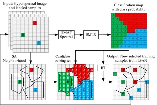
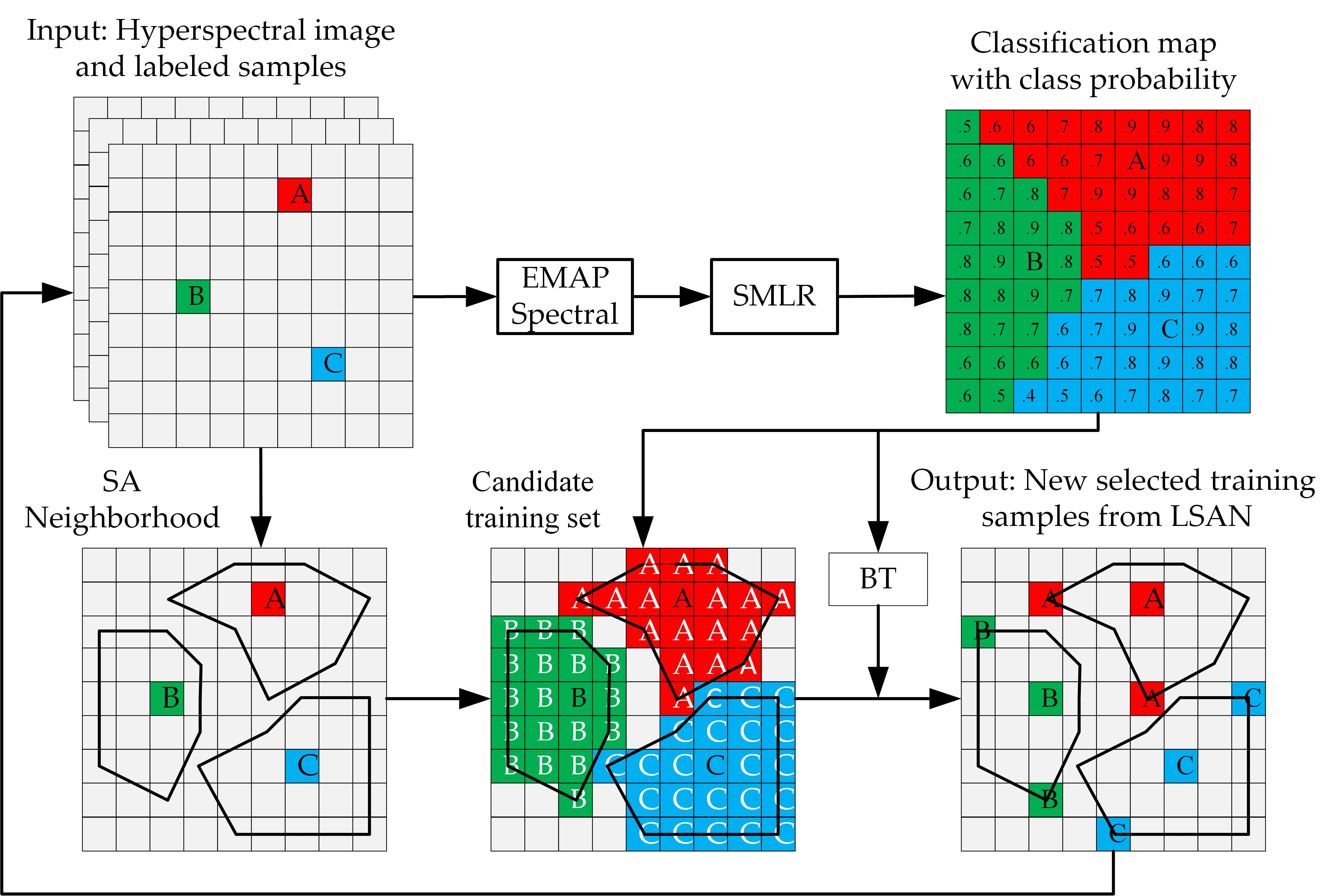
2.3. Unlabeled Samples Selection Method in Proposed SANI-SSL

In the proposed method, we accomplish classification improvement by selecting unlabeled samples from two parts. We first consider the samples from the initial labeled samples’ SA neighborhood (LSAN), which is more reliable and contains abundant unused information. Because the number of labeled training samples is very small, the unlabeled samples in their SA neighborhoods will be trapped in a limited area and the available information is restricted. Thereinafter, the information of the unlabeled samples’ SA neighborhood (uLSAN) is also utilized to select more valuable samples. Figure 2 illustrates the flowchart of the unlabeled samples selection of our SANI-SSL method.

2.3.1. Selecting Unlabeled Samples from LSAN

The selection of unlabeled samples from LSAN is based on two steps. In the first step, a set of candidate unlabeled samples with high confidence is chosen from the SA neighborhood of the labeled samples. In second step, the BT algorithm is adopted on the previously constructed candidate set, in such a way that the most valuable samples from the candidate set can be automatically selected. The specific procedure is shown in Figure 3 for illustrative purpose.
(1)
The construction of candidate training samples
In HSIs classification, there are two basic assumptions for the generation of unlabeled samples for SSL. The first assumption is that samples that have similar spectral characteristics likely belong to the same class. The second assumption is that spatially adjacent pixels likely share same class. Therefore, we integrate the spatial and spectral information into the SSL process in order to construct candidate training samples.
First, we train the spectral-spatial information-based SMLR classifier while using the initial labeled training samples to produce a classification map that contains the probabilities, as mentioned in Section 2.2.1. Second, we extract the SA neighborhoods of the labeled samples. Finally, based on the classification map, we select neighboring unlabeled samples whose predicted class labels are the same as the labels of the corresponding center pixels to constitute the candidate training samples D C L S A N . In this way, an initial pool of candidate training samples with high confidence is established.
(2)
Active learning
The candidate training samples usually contain a large amount of redundant information, since the neighboring pixels carry very similar information to the central pixel. Such a redundancy, although, does not reduce the quality of the classifier, slows down the training phase considerably. AL methods are usually adopted to determine unlabeled training samples that have high uncertainty in order to reduce the redundancies and select the most informative samples from candidate sets. In this paper, we adopt the BT algorithm to evaluate the uncertainty of every pixel by calculating the difference between the two highest probabilities, which is formulated as
x i B T = arg min x i D C L S A N { max k κ   p ( y i = k | x i , ω ) max k κ \ { k M } p ( y i = k | x i , ω ) } ,
where k M represents the class label with the largest posterior probability for x i , and κ \ { k M } represent all of the class labels, excluding k M . The value of BT is between (0, 1), and a smaller value indicates more uncertainty. However, it is important to emphasize that the BT algorithm assumes that only one sample satisfies the condition. Taking the computational complexity into consideration, we select the μ 1 most informative samples from D C L S A N at every iteration. The unlabeled samples selected from LSAN are represented as D u LSAN .

2.3.2. Selecting Unlabeled Samples from uLSAN

The unlabeled samples selected from uLSAN are added to the D T r to make full use of the information in the unlabeled samples and select more representative samples. This part of training samples (denoted as D u uLSAN ) is determined according to three strategies, which are implemented to guarantee the informativeness and confidence. The specific procedures are shown in Figure 4 for illustrative purpose.
(1)
Strategy to ensure informativeness
The BT values of the whole image are computed based on the classification probabilities obtained by training samples. To utilize the feedback information of the available training samples, the most informative samples x u of D T r is used as a benchmark to select new unlabeled samples. More specifically, we define an adaptive interval of uncertainty that takes the BT value of x u to be the lower bound, since a lower BT value indicates less uncertainty. The minimum BT value of D T r is denoted as x u B T , and the adaptive interval is presented as [ x u B T , x u B T + η ] , where η is the length of the interval. Because the training samples are updated every iteration, the x u B T and the interval change every iteration. Subsequently, the samples whose BT values are in the interval are selected as candidate samples D C uLSAN .
(2)
Strategies to ensure confidence
The neighboring pixels in an HSI usually follow the same spectral signatures or features, and the labels of neighboring pixels are highly correlated, which usually arises in the manner of label consistency or label smoothness. In order to ensure high confidence in the label of D C uLSAN , the SANI of D C uLSAN is utilized, and the principle of spatial consistency (SC) is implemented, which demands that the labels of samples are consistent with the mode of the labels of their SA neighborhood. Subsequently, samples that do not meet the SC requirement are excluded from D C uLSAN .
Except for the SC strategy, the ASR method is introduced to predict the labels of the candidate samples with a different mechanism. With the available D T r , the training dictionary is constructed by the EMAP and spectral features of training samples, and the labels of unlabeled samples can be predicted using the ASR. Only candidate samples that satisfy both of the first two conditions are predicted by the ASR to reduce the operation time. Subsequently, samples whose labels assigned by ASR are not same as those under SMLR are excluded from D C uLSAN . Finally, the D u uLSAN are determined by selecting the μ 2 most informative samples from D C uLSAN at every iteration. The samples in D u uLSAN are also added to D T r in order to retrain the classifiers.

3. Experiments

3.1. Datasets Used in the Experiments

In this paper, three public hyperspectral datasets are considered in order to evaluate the performance of the proposed approach.
(1)
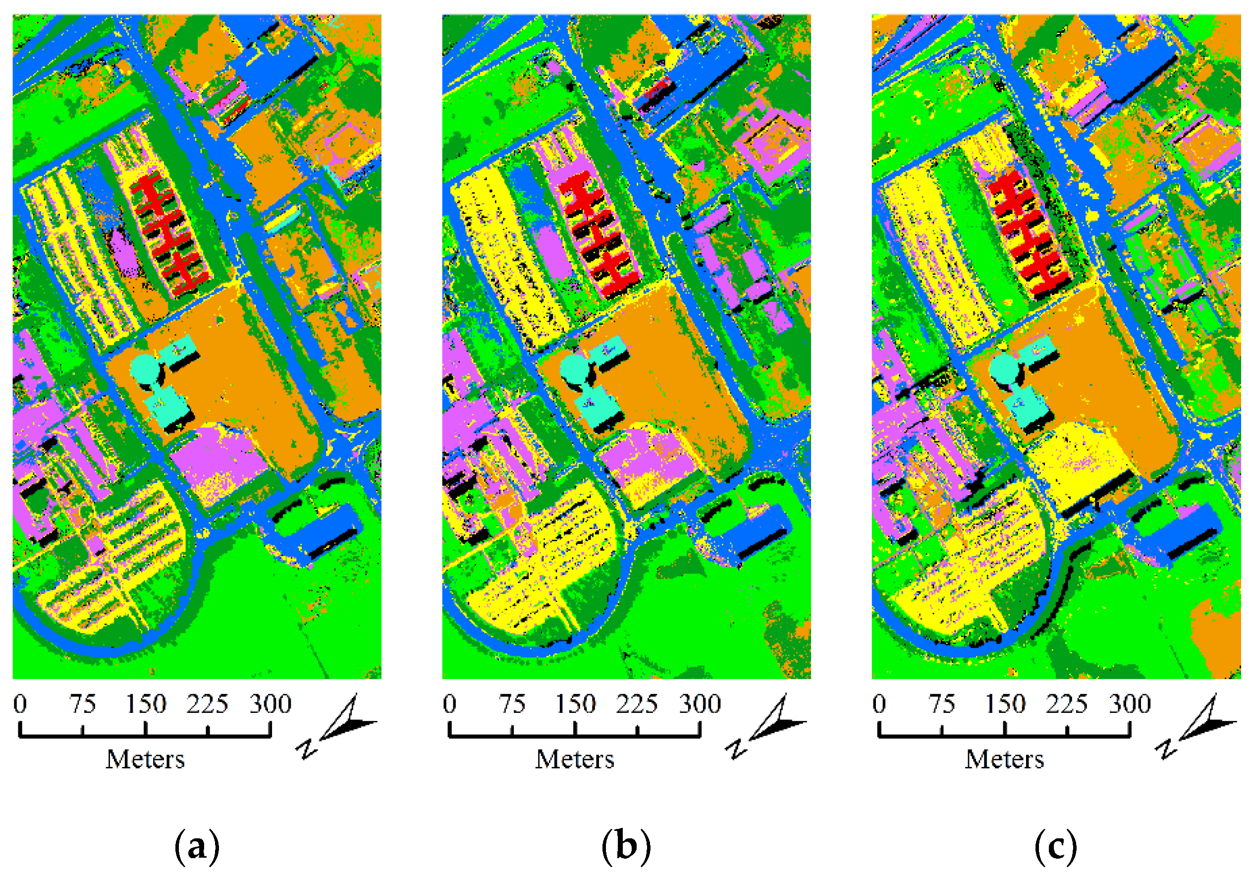
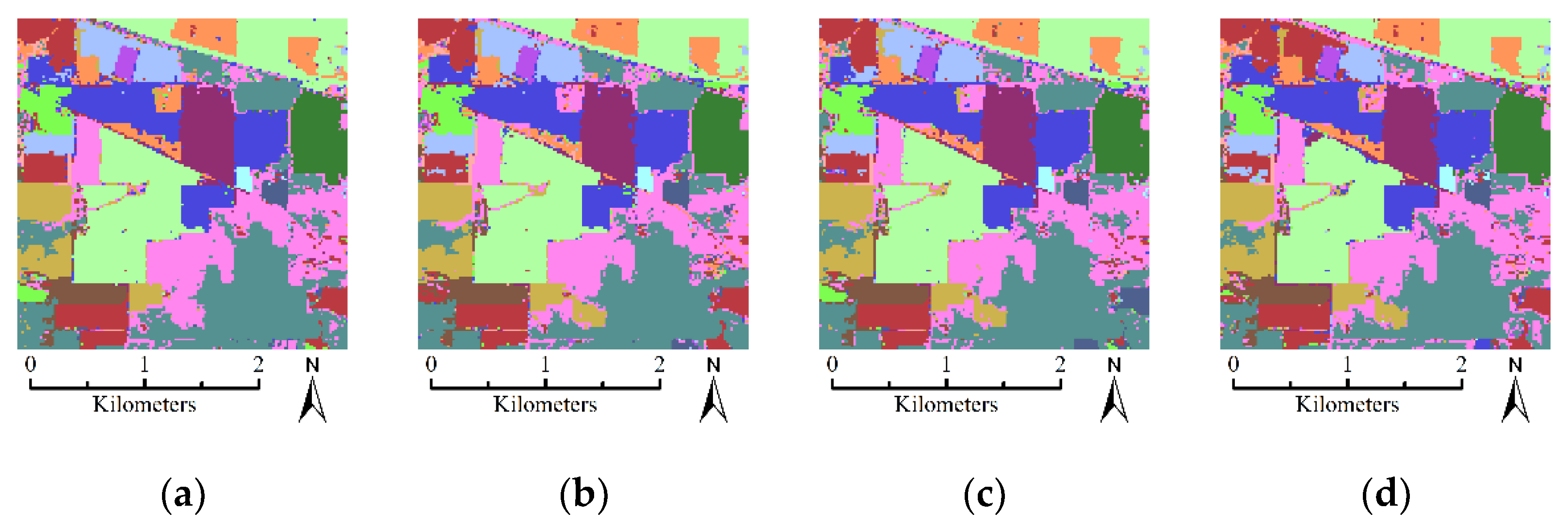
The first hyperspectral dataset used in this paper was acquired by the Airborne Visible/Infrared Imaging Spectrometer (AVIRIS) sensor over a mixed agricultural/forest area in northwestern Indiana in 1992. The dataset contains 145 lines by 145 samples with a spatial resolution of 20 m. It is composed of 224 spectral reflectance bands in the wavelength range from 0.4 um–2.5 um at 10 nm intervals. After an initial screening, the spectral bands were reduced to 200 by removing the bands that cover the region of water absorption. The available ground-truth map contains 10,366 labeled samples with 16 different classes. Figure 5 shows the false color composition image of Indian Pines datasets and ground-truth map.
(2)
The second hyperspectral dataset was acquired by the ROSIS optical sensor over the urban area of the Pavia University, Italy. The dataset contains 610 lines by 310 samples with a spatial resolution of 1.3 m. It comprises 115 spectral channels in the wavelength range of 0.43 um–0.68 µm and 103 spectral bands are used in the experiment after the noisy and water absorption channels were removed. For this dataset, the available ground-truth map contains 42,776 labeled samples with nine classes. Figure 6 shows the false color composition image of Pavia University data and ground-truth map.
(3)
The third hyperspectral dataset was acquired by the AVIRIS sensor over Salinas Valley, California in 1998. The dataset contains 512 lines by 217 samples with a spatial resolution of 3.7 m. It is composed of 224 spectral bands in the wavelength range from 0.4 um–2.5 um, and 204 bands are used in the experiment after noisy and water absorption channels were removed. There are 54,129 samples in total available in the scene which contains 16 classes. Figure 7 shows the false color composition image of Salinas Valley dataset and ground-truth map.

3.2. Experimental Setup

(1)
Spatial information extraction: in this paper, the parameters about EMAP are determined with reference to related work in [20,47]. The thresholds of area attribute are determined according to the scale of the objects, the thresholds of moment of inertia, and standard deviation are determined according to geometry of the objects and the homogeneity of the intensity values of the pixels. Although finer threshold division is conducive to extracting detailed spatial information, the amount of calculation will increase accordingly. For the Indian Pines dataset, the EMAP are extracted while using the attributes area a and moment of inertia i with thresholds λ a = { 100 , 400 , 800 , 1500 } , λ i = { 0.3 , 0.5 , 1 } ; for the Pavia University dataset, the EMAP are extracted using attributes area a and moment of inertia i with thresholds λ a = { 100 , 400 , 800 , 1500 } , λ i = { 0.3 , 0.5 , 1 } ; and, for Salinas Valley dataset, the EMAP are extracted using attributes area a and standard deviation s with thresholds λ a = { 50 , 100 , 500 , 1000 } , λ i = { 0.2 , 0.3 , 0.5 } . The SANI is extracted with the predefined candidate length set H = { 1 , 2 , 3 , 5 , 7 , 9 } for the three datasets.
(2)
Classifier parameter: the kernel width σ = 0.6 , and the degree of sparsity γ = 0.00001 for SMLR.
(3)
Training sets: to evaluate performance of the proposed SANI-SSL method for scenarios with limited labeled samples, only five truly labeled samples per class were randomly chosen from the ground truth for all of the methods in this paper. The number of unlabeled samples is set to be μ 1 + μ 2 = 32 , μ 1 + μ 2 = 18 , μ 1 + μ 2 = 32 for the three datasets, respectively.
(4)
Other settings: the parameter η , which represents the length of the uncertainty interval is intuitively set to 0.25 because we have empirically found that this parameter setting provides better performance and more detailed discussion about η is shown at 3.4.3. The SSL process is executed for 30 iterations. In order to evaluate the performance of our SANI-SSL method quantitatively, the overall accuracy (OA), average accuracy (AA), class-specific accuracies (CA), and kappa coefficient are computed by averaging ten Monte Carlo runs that correspond to independent initial labeled sets.

3.3. Experimental Results with Unlabeled Samples Selected from Only LSAN

In the first experiment, we evaluate the SANI-SSL performance with unlabeled samples selected from only LSAN. In this part, the superpixel (SP) and fixed size (FS) neighborhood information-based SSL methods are also adopted to illustrate the performance of our SANI-SSL method. More specifically, the superpixel information is extracted while using an oversegmentation algorithm, called the entropy rate superpixel (ERS) method [54], and the numbers of superpixels for three datasets are 800, 8000, and 4000, respectively. The fixed size neighborhood information is extracted using a 5 × 5 window for the three datasets. Similar to the SANI-SSL method, the unlabeled samples are selected from the SP-based and FS-based neighborhood of labeled samples.
Figure 8 shows the OA results as a function of the number of unlabeled samples that were obtained by different spatial neighborhood information for the three datasets. As shown in Figure 8, the OAs increase as the number of unlabeled samples increases, which reveal clear advantages for using the spatial neighborhood information to select unlabeled samples. In Figure 8, it can also be seen that the accuracies obtained by the SA based sample selection method are much higher than the accuracies obtained by the SP-based and FS-based methods. The OAs grows rapidly at first since the most informative samples are selected at first and then level off as the valuable unlabeled samples in the neighborhood are running out.
Table 1, Table 2 and Table 3 show the CAs, OAs, AAs, kappa, and running time average statistics obtained by different spatial neighborhood information for the three datasets where the best results are highlighted in bold in order to show the classification results in more detail. As seen in Table 1, Table 2 and Table 3, the proposed SA based method yields better performance than the other methods. This finding is expected, since the neighborhood information determined by the SA method can exploit pixels’ spatial information more accurately and comprehensively. For illustrative purpose, Figure 9, Figure 10 and Figure 11 display the best classification maps obtained using different spatial neighborhood information after 30 iterations for three datasets, along with the corresponding OAs. This experiment reflects the importance the of spatial neighborhood information for selecting the valuable unlabeled samples and the superiority of the SA method for representing the spatial neighborhood information.

3.4. Experimental Results with Unlabeled Samples Selected from LSAN and uLSAN

In the second experiment, we evaluate the performance of SANI-SSL with unlabeled samples selected from both LSAN and uLSAN. As the Figure 8 shows, the classification performance using unlabeled samples selected from LSAN converges after several iterations, which is expected, since the available information of LSAN is limited. Therefore, in our SANI-SSL method, the unlabeled samples that are selected from uLSAN are also added to the training samples. In this part, we conducted several comparison experiments to illustrate some key issues.

3.4.1. The Influence of Unlabeled Samples from uLSAN

To demonstrate the effectiveness of D u uLSAN , we adopted exactly the same number of initial training samples (five per class) and unlabeled samples selected from both LSAN and uLSAN in this part. When considering that the labels of pixels in the LSAN are more reliable, μ 1 is set to 32, 18, and 32 for three datasets at the beginning. In addition, when considering that the valuable information of LSAN is limited, the number of μ 1 decreases by one at each iteration, and the number of μ 2 increases by one correspondingly, to enable the unlabeled samples to be mostly selected from uLSAN when the valuable information in LSAN runs out. Figure 12 shows the OAs of the classification results using unlabeled samples that were selected from both LSAN and uLSAN, which is, our proposed SANI-SSL method. The OAs of classification results using unlabeled samples only from LSAN are also shown for comparison purpose.
The OAs of the two cases are very close to each other at first since the unlabeled samples are mostly selected from LSAN for both cases, the difference between the two methods increases with an increasing number of unlabeled samples, since there are more informative samples in uLSAN than LSAN, as seen in Figure 12. Finally, the OAs increases 1.32%, 1.96%, and 1.21% as compared with the results in Section 3.3 for three datasets, respectively. This experiment reflects that the unlabeled samples from uLSAN can improve the classification performance by improving training samples’ representativeness.

3.4.2. The Influence of the Strategy to Ensure Confidence

In order to further illustrate the importance of the strategies that we adopted to ensure confidence, four groups of comparison experiments were performed, as follows: (1) selecting unlabeled samples using both the SC and ASR strategies, which is, our proposed SANI-SSL method; (2) selecting unlabeled samples only using the SC strategy; (3) selecting unlabeled samples only using the ASR strategy; and, (4) selecting unlabeled samples using neither the SC nor ASR strategy.
Figure 13 shows the OAs of the classification results as a function of the number of unlabeled samples obtained with different strategies for three datasets. When the SC and ASR strategies are employed separately, both of them perform quite well and better than no strategy to ensure confidence for Indian Pines and Salinas Valley datasets, as seen in Figure 13. However, for the Pavia University data, the combination of SC and ASR greatly outperforms other cases, which reveals that both the SC and ASR strategies play an important part in the unlabeled samples’ selection. For the performance difference between three datasets, the main reason is that Pavia University is characterized as a complex spatial structure with stronger heterogeneity, and only one ensured strategy might not guarantee the correctness of the unlabeled samples effectively.
Table 4 shows the detailed OAs, AAs, kappa, and running time results obtained with different strategies to ensure confidence for the three datasets, and the best results are highlighted in bold. It can be seen that the combination of the two confidence strategies provides more satisfactory and stable results; the ASR and SC made almost equal contributions to the confidence of the unlabeled samples, but the ASR was more time-consuming than the SC strategy. Figure 14, Figure 15 and Figure 16 show the best classification map obtained by using different strategies after 30 iterations, along with the corresponding OAs, in order to intuitively illustrate the differences among these methods. The classification results obtained without such ensure strategies have more salt-and-pepper noise than those obtained with both ASR and SC strategies, as can be seen from Figure 14, Figure 15 and Figure 16. It can also be seen that the noise in Figure 14, Figure 15 and Figure 16 is reduced significantly when compared with that in Figure 9, Figure 10 and Figure 11 in Section 3.3. This experiment reflects that the strategies that we adopted are effective to select reliable unlabeled samples and the consuming time is acceptable.

3.4.3. The Influence of the Strategy to Ensure Informativeness

We conducted the experiments using different values of η in order to explore the influence of the parameter η on the classification accuracy. In this part, both of the two strategies to ensure confidence are used. Recall that the BT value is in the range of (0, 1); we set η in the range of (0.05, 0.55) with a 0.05 step size. Figure 17 shows that the OAs of the classification results obtained with different η for three datasets. The classification OAs of three datasets first increases, then reaches the peak value, and finally decreases or keeps the same value, as we can see from Figure 17. It can also be seen that Indian Pines and Salinas Valley datasets are robust to the parameter η and Pavia University dataset is more sensitive to η . This finding is expected, since the larger the value of η is, the more uncertain samples will be included in the candidate sets; the scene in Pavia University is more complex, which makes the labels of the uncertainty samples more prone to error and, thus, affects the final accuracy.

4. Discussion

We reveal some important issues about the proposed SSL methods by conducting several comparison experiments on three hyperspectral datasets.
(1)
The comparison experiment between the SA-, SP-, and FS- based SSL methods shows that our proposed SA-based method performs better than the other two methods. This finding can be explained by the fact that the SA spatial information is beneficial to construct a more representative neighborhood for every pixel. In homogeneous regions of the image, SA has the advantage of representing the neighborhood information comprehensively, while in the heterogeneous region, SA has the advantage of more accurately representing the neighborhood information.
(2)
The comparison experiment between the selection of unlabeled samples from LSAN and uLSAN shows that the uLSAN has great potential in finding valuable samples. This potential could be attributed to two reasons. First, when compared with the limited and high-related information in LSAN, the uLSAN contains abundant undiscovered and unused information, which is helpful in improving the classifier. Second, taking the characteristics of both LSAN and uLSAN into full consideration, the unlabeled samples are selected from these two regions at generally appropriate time by adjusting the number of unlabeled samples from both regions.
(3)
The influence of different strategies confidence to ensure on the classification accuracy is analyzed in Section 3.4.2, and the result shows that the two strategies can ensure that the selected samples are assigned by correct labels, and the SC strategy shows better performance in computational efficiency. The influence of the informativeness parameter η on the classification accuracy is analyzed by conducting experiments using different value of η , and the best performance is acquired by setting η to 0.25 according to the results of three datasets. As for the difference in performance of the three datasets, the main reason is that the spatial characteristics in the datasets are different. The main ground objects of Indian Pines and Salinas Valley datasets are cropland, which have larger spatial scale and regular distribution. However, for the urban scene in Pavia University dataset, the spatial distribution is more complicated; therefore, more stringent requirements on the strategies need to be satisfied in order to achieve satisfactory results.
We make a comparison between the proposed SANI-SSL method and the following spectral-spatial-based SSL methods for HSIs classification to further evaluate the performance of the proposed method: (1) tri-training based semi-supervised learning (TT-SSL) proposed in [55]; (2) generative adversarial networks based semi-supervised learning (GANs-SSL) proposed in [25]; and, (3) superpixel and density peak based semi-supervised learning (SDP-SSL) proposed in [30]. Table 5 shows the classification OAs, AAs, and kappa coefficient of our proposed SANI-SSL method in comparison with those of the above methods using five truly labeled samples per class for the Indian Pines and Pavia University datasets (some of the above methods did not use Salinas Valley dataset). It can be seen from Table 5 that the performance of SANI-SSL is better than the other spectral-spatial based SSL methods, which confirms the effectiveness of our proposed method.

5. Conclusions

In this paper, we have presented a SANI based SSL method for HSIs classification, which exploits the SANI of both labeled and unlabeled samples in order to make full use of the spectral-spatial information of the whole image. The EMAP-based spatial information is extracted and fused with spectral information firstly to enhance the discriminability of the different classes, and the SA-based spatial neighborhood information is used to select unlabeled samples. The novelty of this paper is that we selected unlabeled samples not only using the SANI of truly labeled samples, but also utilizing the SANI of unlabeled samples. For the unlabeled samples selected from LSAN, the SANI is utilized in order to guarantee the confidence of the unlabeled samples, and the BT algorithm is adopted to guarantee the informativeness. For the unlabeled samples selected from uLSAN, the SANI and classifier combination methods are utilized to guarantee the confidence, and a novel adaptive interval method is proposed to guarantee the informativeness. The proposed method was tested on Indian Pines, Pavia University, and Salinas Valley datasets, and the comparison with other spectral-spatial-based SSL methods (i.e., TT-SSL, GANs-SSL, and SDP-SSL) has demonstrated the superiority and effectiveness of the proposed SANI-based SSL method.
In future work, we would consider combining the SA-based spatial information with spectral information in order to improve the performance of the classifier, and investigating the influence of the scale of spatial features on HSIs classification.

Author Contributions

Y.H. and R.A. conceived the conceptualization and designed the experiments; Y.H. analyzed the data; Y.H. and R.A. wrote the main manuscript text; Y.H., R.A., B.W., F.X. and F.J. reviewed and edited the manuscript. All authors have read and agreed to the published version of the manuscript.

Funding

This research was funded by National Natural Science Foundation of China (Grant No. 41871326, No. 41271361).

Acknowledgments

The authors would like to thank the reviewers and editors for their valuable comments and suggestions.

Conflicts of Interest

The authors declare no conflict of interest.

References

  1. Luo, Y.H.; Tao, Z.P.; Ke, G.; Wang, M.Z. The Application Research of Hyperspectral Remote Sensing Technology in Tailing Mine Environment Pollution Supervise Management. In Proceedings of the 2012 2nd International Conference on Remote Sensing, Environment and Transportation Engineering, Nanjing, China, 1–3 June 2012; pp. 1–4. [Google Scholar]
  2. Tong, Q.; Zhang, B.; Zheng, L. Hyperspectral Remote Sensing: The Principle, Technology and Application; Higher Education Press: Beijing, China, 2006. [Google Scholar]
  3. Majdar, R.S.; Ghassemian, H. A probabilistic SVM approach for hyperspectral image classification using spectral and texture features. Int. J. Remote Sens. 2017, 38, 4265–4284. [Google Scholar] [CrossRef]
  4. Hughes, G. On the mean accuracy of statistical pattern recognizers. IEEE Trans. Inf. Theory 1968, 14, 55–63. [Google Scholar] [CrossRef] [Green Version]
  5. Du, P.; Xia, J.; Xue, Z.; Tan, K.; Su, H.; Bao, R. Review of hyperspectral remote sensing image classification. J. Remote Sens. 2016, 20, 236–256. [Google Scholar]
  6. Ballanti, L.; Blesius, L.; Hines, E.; Kruse, B. Tree Species Classification Using Hyperspectral Imagery: A Comparison of Two Classifiers. Remote Sens. 2016, 8, 445. [Google Scholar] [CrossRef] [Green Version]
  7. Yu, H.; Gao, L.; Li, J.; Li, S.S.; Zhang, B.; Benediktsson, J.A. Spectral-Spatial Hyperspectral Image Classification Using Subspace-Based Support Vector Machines and Adaptive Markov Random Fields. Remote Sens. 2016, 8, 355. [Google Scholar] [CrossRef] [Green Version]
  8. Cao, F.; Yang, Z.; Ren, J.; Ling, W.K.; Zhao, H.; Marshall, S. Extreme Sparse Multinomial Logistic Regression: A Fast and Robust Framework for Hyperspectral Image Classification. Remote Sens. 2017, 9, 1255. [Google Scholar] [CrossRef] [Green Version]
  9. Li, J.; Bioucas-Dias, J.M.; Plaza, A. Spectral-Spatial Hyperspectral Image Segmentation Using Subspace Multinomial Logistic Regression and Markov Random Fields. IEEE Trans. Geosci. Remote Sens. 2012, 50, 809–823. [Google Scholar] [CrossRef]
  10. Li, J.; Gamba, P.; Plaza, A. A Novel Semi-Supervised Method for Obtaining Finer Resolution Urban Extents Exploiting Coarser Resolution Maps. IEEE J. Sel. Top. Appl. Earth Obs. Remote Sens. 2014, 7, 4276–4287. [Google Scholar] [CrossRef]
  11. Chen, C.; Li, W.; Su, H.; Liu, K. Spectral-Spatial Classification of Hyperspectral Image Based on Kernel Extreme Learning Machine. Remote Sens. 2014, 6, 5795–5814. [Google Scholar] [CrossRef] [Green Version]
  12. Li, Y.; Zhang, H.; Shen, Q. Spectral-Spatial Classification of Hyperspectral Imagery with 3D Convolutional Neural Network. Remote Sens. 2017, 9, 67. [Google Scholar] [CrossRef] [Green Version]
  13. Mirzapour, F.; Ghassemian, H. Improving hyperspectral image classification by combining spectral, texture, and shape features. Int. J. Remote Sens. 2015, 36, 1070–1096. [Google Scholar] [CrossRef]
  14. Huang, X.; Liu, X.; Zhang, L. A Multichannel Gray Level Co-Occurrence Matrix for Multi/Hyperspectral Image Texture Representation. Remote Sens. 2014, 6, 8424–8445. [Google Scholar] [CrossRef] [Green Version]
  15. Li, J.; Xi, B.; Li, Y.; Du, Q.; Wang, K. Hyperspectral Classification Based on Texture Feature Enhancement and Deep Belief Networks. Remote Sens. 2018, 10, 396. [Google Scholar] [CrossRef] [Green Version]
  16. Wang, Y.; Zhang, Y.; Song, H. A Spectral-Texture Kernel-Based Classification Method for Hyperspectral Images. Remote Sens. 2016, 8, 919. [Google Scholar] [CrossRef] [Green Version]
  17. Zhang, B.; Li, S.; Jia, X.; Gao, L.; Peng, M. Adaptive Markov Random Field Approach for Classification of Hyperspectral Imagery. IEEE Geosci. Remote Sens. Lett. 2011, 8, 973–977. [Google Scholar] [CrossRef]
  18. Andrejchenko, V.; Liao, W.; Philips, W.; Scheunders, P. Decision Fusion Framework for Hyperspectral Image Classification Based on Markov and Conditional Random Fields. Remote Sens. 2019, 11, 624. [Google Scholar] [CrossRef] [Green Version]
  19. Cao, X.; Xu, Z.; Meng, D. Spectral-Spatial Hyperspectral Image Classification via Robust Low-Rank Feature Extraction and Markov Random Field. Remote Sens. 2019, 11, 1565. [Google Scholar] [CrossRef] [Green Version]
  20. Dalla Mura, M.; Benediktsson, J.A.; Waske, B.; Bruzzone, L. Extended profiles with morphological attribute filters for the analysis of hyperspectral data. Int. J. Remote Sens. 2010, 31, 5975–5991. [Google Scholar] [CrossRef]
  21. Liang, H.; Li, Q. Hyperspectral Imagery Classification Using Sparse Representations of Convolutional Neural Network Features. Remote Sens. 2016, 8, 99. [Google Scholar] [CrossRef] [Green Version]
  22. Sun, Y.; Wang, S.; Liu, Q.; Hang, R.; Liu, G. Hypergraph Embedding for Spatial-Spectral Joint Feature Extraction in Hyperspectral Images. Remote Sens. 2017, 9, 506–519. [Google Scholar]
  23. Andekah, Z.A.; Naderan, M.; Akbarizadeh, G.; IEEE. Semi-Supervised Hyperspectral Image Classification using Spatial-Spectral Features and Superpixel-Based Sparse Codes. In Proceedings of the 25th Iranian Conference on Electrical Engineering, Teheran, Iran, 2–4 May 2017; pp. 2229–2234. [Google Scholar]
  24. Fu, Q.; Yu, X.; Zhang, P.; Wei, X. Semi-supervised ELM combined with spectral-spatial featuresfor hyperspectral imagery classification. J. Huazhong Univ. Sci. Technol. Nat. Sci. 2017, 45, 89–93. [Google Scholar]
  25. He, Z.; Liu, H.; Wang, Y.; Hu, J. Generative Adversarial Networks-Based Semi-Supervised Learning for Hyperspectral Image Classification. Remote Sens. 2017, 9, 1042. [Google Scholar] [CrossRef] [Green Version]
  26. Tan, K.; Li, E.; Du, Q.; Du, P. An efficient semi-supervised classification approach for hyperspectral imagery. ISPRS J. Photogramm. Remote Sens. 2014, 97, 36–45. [Google Scholar] [CrossRef]
  27. Dopido, I.; Li, J.; Marpu, P.R.; Plaza, A.; Bioucas Dias, J.M.; Benediktsson, J.A. Semisupervised Self-Learning for Hyperspectral Image Classification. IEEE Trans. Geosci. Remote Sens. 2013, 51, 4032–4044. [Google Scholar] [CrossRef] [Green Version]
  28. Wu, Y.; Mu, G.F.; Qin, C.; Miao, Q.G.; Ma, W.P.; Zhang, X.R. Semi-Supervised Hyperspectral Image Classification via Spatial-Regulated Self-Training. Remote Sens. 2020, 12, 159. [Google Scholar] [CrossRef] [Green Version]
  29. Wang, L.; Hao, S.; Wang, Q.; Wang, Y. Semi-supervised classification for hyperspectral imagery based on spatial-spectral Label Propagation. ISPRS J. Photogramm. Remote Sens. 2014, 97, 123–137. [Google Scholar] [CrossRef]
  30. Liu, C.; Li, J.; He, L. Superpixel-Based Semisupervised Active Learning for Hyperspectral Image Classification. IEEE J. Sel. Top. Appl. Earth Obs. Remote Sens. 2019, 12, 357–370. [Google Scholar] [CrossRef]
  31. Balasubramaniam, R.; Namboodiri, S.; Nidamanuri, R.R.; Gorthi, R.K.S.S. Active Learning-Based Optimized Training Library Generation for Object-Oriented Image Classification. IEEE Trans. Geosci. Remote Sens. 2018, 56, 575–585. [Google Scholar] [CrossRef]
  32. Zhao, Y.; Su, F.; Yan, F. Novel Semi-Supervised Hyperspectral Image Classification Based on a Superpixel Graph and Discrete Potential Method. Remote Sens. 2020, 12, 1528–1547. [Google Scholar] [CrossRef]
  33. Tan, K.; Hu, J.; Li, J.; Du, P.J. A novel semi-supervised hyperspectral image classification approach based on spatial neighborhood information and classifier combination. ISPRS J. Photogramm. Remote Sens. 2015, 105, 19–29. [Google Scholar] [CrossRef]
  34. Luo, T.; Kramer, K.; Goldgof, D.B.; Hall, L.O.; Samson, S.; Remsen, A.; Hopkins, T. Active learning to recognize multiple types of plankton. J. Mach. Learn. Res. 2005, 6, 589–613. [Google Scholar]
  35. Li, J.; Bioucas-Dias, J.M.; Plaza, A. Semisupervised Hyperspectral Image Segmentation Using Multinomial Logistic Regression with Active Learning. IEEE Trans. Geosci. Remote Sens. 2010, 48, 4085–4098. [Google Scholar] [CrossRef] [Green Version]
  36. Li, J.; Bioucas-Dias, J.M.; Plaza, A. Hyperspectral Image Segmentation Using a New Bayesian Approach with Active Learning. IEEE Trans. Geosci. Remote Sens. 2011, 49, 3947–3960. [Google Scholar] [CrossRef] [Green Version]
  37. Li, J.; Bioucas-Dias, J.M.; Plaza, A. Spectral-Spatial Classification of Hyperspectral Data Using Loopy Belief Propagation and Active Learning. IEEE Trans. Geosci. Remote Sens. 2013, 51, 844–856. [Google Scholar] [CrossRef]
  38. Wang, L.; Hao, S.; Wang, Y.; Lin, Y.; Wang, Q. Spatial-Spectral Information-Based Semisupervised Classification Algorithm for Hyperspectral Imagery. IEEE J. Sel. Top. Appl. Earth Obs. Remote Sens. 2014, 7, 3577–3585. [Google Scholar] [CrossRef]
  39. Shi, Q.; Liu, X.; Huang, X. An Active Relearning Framework for Remote Sensing Image Classification. IEEE Trans. Geosci. Remote Sens. 2018, 56, 3468–3486. [Google Scholar] [CrossRef]
  40. Shu, W.; Liu, P.; He, G.; Wang, G. Hyperspectral Image Classification Using Spectral-Spatial Features with Informative Samples. IEEE Access 2019, 7, 20869–20878. [Google Scholar] [CrossRef]
  41. Pesaresi, M.; Benediktsson, J.A. A new approach for the morphological segmentation of high-resolution satellite imagery. IEEE Trans. Geosci. Remote Sens. 2001, 39, 309–320. [Google Scholar] [CrossRef] [Green Version]
  42. Foi, A.; Katkovnik, V.; Egiazarian, K. Pointwise shape-adaptive DCT for high-quality denoising and deblocking of grayscale and color images. IEEE Trans. Image Process. 2007, 16, 1395–1411. [Google Scholar] [CrossRef]
  43. Yang, J.; Qian, J. Joint Collaborative Representation with Shape Adaptive Region and Locally Adaptive Dictionary for Hyperspectral Image Classification. IEEE Geosci. Remote Sens. Lett. 2020, 17, 671–675. [Google Scholar] [CrossRef]
  44. Xue, Z.; Du, P.; Li, J.; Su, H. Simultaneous Sparse Graph Embedding for Hyperspectral Image Classification. IEEE Trans. Geosci. Remote Sens. 2015, 53, 6114–6133. [Google Scholar] [CrossRef]
  45. Du, P.; Xue, Z.; Li, J.; Plaza, A. Learning Discriminative Sparse Representations for Hyperspectral Image Classification. IEEE J. Sel. Top. Signal. Process. 2015, 9, 1089–1104. [Google Scholar] [CrossRef]
  46. Kayabol, K. Approximate Sparse Multinomial Logistic Regression for Classification. IEEE Trans. Pattern Anal. Mach. Intell. 2020, 42, 490–493. [Google Scholar] [CrossRef]
  47. Li, J.; Huang, X.; Gamba, P.; Bioucas-Dias, J.M.; Zhang, L.; Benediktsson, J.A.; Plaza, A. Multiple Feature Learning for Hyperspectral Image Classification. IEEE Trans. Geosci. Remote Sens. 2015, 53, 1592–1606. [Google Scholar] [CrossRef] [Green Version]
  48. Dopido, I.; Li, J.; Plaza, A.; Bioucas-Dias, J.M.; IEEE. A New Semi-supervised Approach for Hyperspectral Image Classification with Different Active Learnings Strategies. In Proceedings of the 2012 4th Workshop on Hyperspectral Image and Signal Processing, Shangai, China, 4–7 June 2012. [Google Scholar]
  49. Böhning, D. Multinomial logistic regression algorithm. Ann. Inst. Stat. Math. 1992, 44, 197–200. [Google Scholar] [CrossRef]
  50. Camps-Valls, G.; Bruzzone, L. Kernel-based methods for hyperspectral image classification. IEEE Trans. Geosci. Remote Sens. 2005, 43, 1351–1362. [Google Scholar] [CrossRef]
  51. Bioucasdias, B.J.; Figueiredo, M. Logistic Regression via Variable Splitting and Augmented Lagrangian Tools; Technical Report; Instituto Superior Técnico: Lisboa, Portugal, 2009. [Google Scholar]
  52. Fang, L.; Li, S.; Kang, X.; Benediktsson, J.A. Spectral-Spatial Hyperspectral Image Classification via Multiscale Adaptive Sparse Representation. IEEE Trans. Geosci. Remote Sens. 2014, 52, 7738–7749. [Google Scholar] [CrossRef]
  53. Melgani, F.; Bruzzone, L. Classification of hyperspectral remote sensing images with support vector machines. IEEE Trans. Geosci. Remote Sens. 2004, 42, 1778–1790. [Google Scholar] [CrossRef] [Green Version]
  54. Liu, M.Y.; Tuzel, O.; Ramalingam, S.; Chellappa, R.; IEEE. Entropy Rate Superpixel Segmentation. In Proceedings of the IEEE Conference on Computer Vision and Pattern Recognition, Washington, DC, USA, 20–25 June 2011. [Google Scholar]
  55. Tan, K.; Zhu, J.; Du, Q.; Wu, L.; Du, P. A Novel Tri-Training Technique for Semi-Supervised Classification of Hyperspectral Images Based on Diversity Measurement. Remote Sens. 2016, 8, 749. [Google Scholar] [CrossRef] [Green Version]
Figure 1. (a) Diagram of an example shape adaptive (SA) region. The red block denotes the central pixel, the dark gray block denotes the length in the eight directions, and the light gray block denotes the SA neighborhood; (bd) are examples of the SA neighborhood for the Indian Pines data, part of the Pavia University data and part of the Salinas Valley data, respectively.
Remotesensing 12 02976 g001
Figure 2. Flowchart of the unlabeled samples selection of our proposed shape adaptive neighborhood information based semi-supervised learning (SANI-SSL).
Remotesensing 12 02976 g002
Figure 3. Flowchart for the selection of unlabeled samples from labeled samples’ SA neighborhood (LSAN).
Remotesensing 12 02976 g003
Figure 4. Flowchart for the selection of unlabeled samples from unlabeled samples’ SA neighborhood (uLSAN).
Remotesensing 12 02976 g004
Figure 5. (a) The false color composition image of Indian Pines dataset; and, (b) the ground truth map of Indian Pines dataset.
Remotesensing 12 02976 g005
Figure 6. (a) The false color composition image of Pavia University dataset; and, (b) the ground truth map of Pavia University dataset.
Remotesensing 12 02976 g006
Figure 7. (a) The false color composition image of Salinas Valley dataset; and, (b) the ground truth map of Salinas Valley dataset.
Remotesensing 12 02976 g007
Figure 8. Overall accuracies (OAs) as a function of the number of unlabeled samples with unlabeled samples selected from the SA-, SP-, and FS- based neighborhood for the three datasets: (a) Indian Pines dataset; (b) Pavia University dataset; and, (c) Salinas Valley dataset.
Remotesensing 12 02976 g008
Figure 9. Classification maps of Indian Pines dataset obtained by using different spatial neighborhood information: (a) SA (86.82%); (b) SP (82.55%); and, (c) FS (84.71%).
Remotesensing 12 02976 g009
Figure 10. Classification maps of Pavia University dataset obtained by using different spatial neighborhood information: (a) SA (92.69%); (b) SP (88.92%); and, (c) FS (90.41%).
Remotesensing 12 02976 g010
Figure 11. Classification maps of Salinas Valley dataset obtained by using different spatial neighborhood information: (a) SA (96.06%); (b) SP (94.91%); (c) FS (94.48%).
Remotesensing 12 02976 g011
Figure 12. OAs as a function of the number of unlabeled samples with unlabeled samples selected from only LSAN and from uLSAN, LSAN simultaneously for the (a) Indian Pines dataset, (b) Pavia University dataset, and (c) Salinas Valley dataset.
Remotesensing 12 02976 g012
Figure 13. OAs as a function of the number of unlabeled samples obtained by using different strategies to ensure confidence for the (a) Indian Pines dataset, (b) Pavia University dataset, and (c) Salinas Valley dataset.
Remotesensing 12 02976 g013
Figure 14. Classification maps obtained by using different strategies to ensure confidence for Indian Pines dataset: (a) with SC and ASR (90.90%); (b) with SC (90.61%); (c) with ASR (90.16%); and, (d) without SC or ASR (87.76%).
Remotesensing 12 02976 g014
Figure 15. Classification maps obtained by using different strategies to ensure confidence for Pavia University dataset: (a) with SC and ASR (95.85%); (b) with SC (91.72%); (c) with ASR (93.04%); and, (d) without SC or ASR (86.03%).
Remotesensing 12 02976 g015
Figure 16. Classification maps obtained by using different strategies to ensure confidence for Salinas Valley dataset: (a) with SC and ASR (97.24%); (b) with SC (96.97%); (c) with ASR (96.38%); and, (d) without SC or ASR (95.51%).
Remotesensing 12 02976 g016
Figure 17. The influence of the parameter η on the OAs of classification results.
Remotesensing 12 02976 g017
Table 1. Class-specific accuracies (CAs), OAs, average accuracies (AAs), kappa (as a percentage, with the standard deviation in brackets), and running time average statistics obtained with unlabeled samples selected from the SA-, SP-, and FS- based neighborhood for Indian Pines dataset.
ClassNumber of Testing SamplesSASPFS
Alfalfa4991.63 ± (5.66)91.02 ± (5.49)92.45 ± (6.13)
Corn-Notill142969.66 ± (10.72)64.85 ± (8.90)68.01 ± (7.97)
Corn-Mintill82972.98 ± (11.77)62.36 ± (11.51)65.11 ± (8.32)
Corn22979.87 ± (11.77)93.49 ± (6.42)87.60 ± (7.80)
Grass-Pasture49281.36 ± (6.16)78.01 ± (5.57)80.08 ± (5.53)
Grass-Trees74296.73 ± (1.38)87.80 ± (8.78)95.22 ± (3.72)
Grass-Pasture-Mowed2196.67 ± (3.05)98.57 ± (2.18)99.05 ± (1.90)
Hay-Windrowed484100.00 ± (0.00)99.77 ± (0.22)99.67 ± (0.28)
Oats15100.00 ± (0.00)100.00 ± (0.00)100.00 ± (0.00)
Soybean-Notill96381.73 ± (5.00)80.82 ± (5.08)80.08 ± (4.60)
Soybean-Mintill246381.12 ± (6.08)75.54 ± (8.95)75.28 ± (10.36)
Soybean-Clean60978.83 ± (13.92)60.31 ± (18.88)70.89 ± (17.34)
Wheat20799.52 ± (2.22)99.23 ± (0.24)99.52 ± (0.22)
Woods128991.61 ± (9.32)89.34 ± (10.42)91.39 ± (8.91)
Buildings-Grass-Trees-Drives37585.79 ± (10.16)87.76 ± (10.19)87.44 ± (10.34)
Stone-Steel-Towers9097.22 ± (2.12)96.44 ± (4.38)98.78 ± (1.26)
OA82.90 ± (2.37)78.12 ± (3.39)80.05 ± (3.35)
AA87.79 ± (1.80)85.33 ± (2.02)86.91 ± (1.79)
Kappa80.67 ± (2.63)75.46 ± (3.69)77.59 ± (3.66)
Time(s)242236237
Table 2. CAs, OAs, AAs, kappa (as a percentage, with the standard deviation in brackets), and running time average statistics obtained with unlabeled samples selected from SA-, SP-, and FS- based neighborhood for Pavia University dataset.
ClassNumber of Testing SamplesSASPFS
Asphalt662692.79 ± (3.26)93.62 ± (6.50)96.02 ± (2.83)
Meadows18,64481.53 ± (6.82)75.95 ± (6.35)73.91 ± (6.67)
Gravel209492.95 ± (7.12)90.21 ± (8.08)91.63 ± (4.71)
Trees305986.54 ± (6.14)86.90 ± (5.07)91.01 ± (5.07)
Painted Metal Sheets134094.31 ± (6.47)97.49 ± (3.71)98.07 ± (2.44)
Bare Soil502493.64 ± (5.09)92.87 ± (5.56)94.22 ± (5.10)
Bitumen132599.88 ± (0.08)99.55 ± (0.66)99.71 ± (0.35)
Self-Blocking Bricks367796.32 ± (2.90)96.69 ± (2.48)96.96 ± (3.03)
Shadows94297.26 ± (4.28)78.94 ± (12.15)84.21 ± (11.38)
OA88.21 ± (2.55)85.42 ± (2.45)85.59 ± (2.80)
AA92.80 ± (1.93)90.25 ± (1.37)91.75 ± (1.76)
Kappa84.92 ± (3.07)81.59 ± (2.89)81.85 ± (3.33)
Time(s)267263258
Table 3. CAs, OAs, AAs, kappa (as a percentage, with the standard deviation in brackets), and running time average statistics obtained with unlabeled samples selected from SA-, SP-, and FS- based neighborhood for Salinas Valley dataset.
ClassNumber of Testing SamplesSASPFS
Brocoli_Green_Weeds_1200499.89 ± (0.14)99.50 ± (0.46)99.31 ± (0.71)
Brocoli_Green_Weeds_2372199.29 ± (0.26)99.38 ± (0.28)99.44 ± (0.26)
Fallow197193.28 ± (15.64)92.57 ± (16.59)93.19 ± (16.38)
Fallow_Rough_Plow138997.27 ± (4.41)98.60 ± (2.39)99.25 ± (0.90)
Fallow_Smooth267392.79 ± (4.81)97.01 ± (2.01)97.34 ± (0.94)
Stubble395498.21 ± (1.65)96.46 ± (2.22)96.78 ± (2.52)
Celery357498.82 ± (0.70)99.39 ± (0.30)99.39 ± (0.31)
Grapes_Untrained11,26684.98 ± (3.21)78.83 ± (6.01)76.95 ± (8.55)
Soil_Vinyard_Develop619899.75 ± (0.32)99.07 ± (1.29)99.65 ± (0.61)
Corn_Senesced_Green_Weeds327396.02 ± (2.62)92.62 ± (7.43)92.06 ± (7.96)
Lettuce_Romaine_4 wk106395.50 ± (12.18)97.54 ± (1.60)97.48 ± (1.47)
Lettuce_Romaine_5 wk192296.15 ± (5.42)97.30 ± (6.42)99.99 ± (0.02)
Lettuce_Romaine_6 wk91199.08 ± (0.50)99.13 ± (0.97)99.09 ± (0.74)
Lettuce_Romaine_7 wk106593.05 ± (7.05)89.92 ± (7.10)92.08 ± (6.32)
Vinyard_Untrained726391.91 ± (5.61)91.01 ± (4.46)91.47 ± (4.11)
Vinyard_Vertical_Trellis180296.03 ± (2.33)96.45 ± (2.97)94.51 ± (2.88)
OA94.07 ± (1.40)92.53± (1.78)92.38 ± (2.07)
AA95.75 ± (1.45)95.30 ± (1.49)95.50 ± (1.28)
Kappa93.41 ± (1.55)91.72 ± (1.96)91.55 ± (2.29)
Time(s)425430401
Table 4. OA, AA, kappa (as a percentage, with the standard deviation in brackets), and running time average statistics obtained by using different strategies to ensure confidence for three datasets.
Strategy to Ensure Confidencewith SC and ASRwith SCwith ASRwithout SC or ASR
Indian PinesOA (%)84.22 ± (3.20)84.56 ± (2.51)84.20 ± (3.12)83.19 ± (2.83)
AA (%)88.55 ± (2.32)88.47 ± (2.00)88.29 ± (2.46)87.64 ± (2.04)
Kappa (%)82.14 ± (3.59)82.52 ± (2.80)82.12 ± (3.49)80.98 ± (3.16)
Time(s)289244367269
Pavia UniversityOA (%)90.17 ± (4.87)87.39 ± (3.27)87.27 ± (4.39)81.52 ± (3.63)
AA (%)90.81 ± (3.64)88.30 ± (1.94)90.34 ± (1.80)83.00 ± (2.10)
Kappa (%)87.29 ± (6.03)83.76 ± (3.91)83.68 ± (5.34)76.42 ± (4.20)
Time(s)441425565258
Salinas ValleyOA (%)95.28 ± (1.51)95.10 ± (1.04)94.62 ± (1.48)92.30 ± (2.25)
AA (%)96.76 ± (1.03)96.49 ± (1.14)96.52 ± (1.15)94.58 ± (1.72)
Kappa (%)94.75 ± (1.68)94.56 ± (1.15)94.02 ± (1.64)91.45 ± (2.50)
Time(s)571367640394
Table 5. Comparison of OAs, AAs, and kappa (as a percentage) between the proposed SANI-SSL method and other spectral-spatial information-based SSL methods.
DatasetsTT-SSLGANs-SSLSDP-SSLSANI-SSL
Indian PinesOA77.5575.6282.6684.22
AA85.1681.0588.1288.55
Kappa74.7972.2380.2782.14
Pavia UniversityOA82.5577.9484.2090.17
AA88.6981.3689.1490.81
Kappa78.0171.8279.8687.29

