Article

Detection of Italian Ryegrass in Wheat and Prediction of Competitive Interactions Using Remote-Sensing and Machine-Learning Techniques

1
Department of Soil and Crop Sciences, Texas A&M University, College Station, TX 77840, USA
2
Eastern Shore Agricultural Research and Extension Center, Virginia Tech, Painter, VA 23420, USA
3
Department of Crop and Soil Sciences, Washington State University, Pullman, WA 646420, USA
*
Author to whom correspondence should be addressed.
Remote Sens. 2020, 12(18), 2977; https://doi.org/10.3390/rs12182977
Submission received: 3 August 2020 / Revised: 6 September 2020 / Accepted: 11 September 2020 / Published: 13 September 2020

Abstract

:
Italian ryegrass (Lolium perenne ssp. multiflorum (Lam) Husnot) is a troublesome weed species in wheat (Triticum aestivum) production in the United States, severely affecting grain yields. Spatial mapping of ryegrass infestation in wheat fields and early prediction of its impact on yield can assist management decision making. In this study, unmanned aerial systems (UAS)-based red, green and blue (RGB) imageries acquired at an early wheat growth stage in two different experimental sites were used for developing predictive models. Deep neural networks (DNNs) coupled with an extensive feature selection method were used to detect ryegrass in wheat and estimate ryegrass canopy coverage. Predictive models were developed by regressing early-season ryegrass canopy coverage (%) with end-of-season (at wheat maturity) biomass and seed yield of ryegrass, as well as biomass and grain yield reduction (%) of wheat. Italian ryegrass was detected with high accuracy (precision = 95.44 ± 4.27%, recall = 95.48 ± 5.05%, F-score = 95.56 ± 4.11%) using the best model which included four features: hue, saturation, excess green index, and visible atmospheric resistant index. End-of-season ryegrass biomass was predicted with high accuracy (R2 = 0.87), whereas the other variables had moderate to high accuracy levels (R2 values of 0.74 for ryegrass seed yield, 0.73 for wheat biomass reduction, and 0.69 for wheat grain yield reduction). The methodology demonstrated in the current study shows great potential for mapping and quantifying ryegrass infestation and predicting its competitive response in wheat, allowing for timely management decisions.

Graphical Abstract

1. Introduction

Italian ryegrass (Lolium perenne ssp. multiflorum (Lam) Husnot) is one of the most problematic weeds in wheat (Triticum aestivum L.) production in the United States (U.S.) [1]. Italian ryegrass is a cool-season winter annual weed that thrives best under a temperature range of 20 to 25 °C. It has faster leaf expansion rate than wheat and its competition can negatively impact tiller production, uptake of soil nutrients, photosynthesis and overall growth of wheat, resulting in significant crop yield loss [2,3]. Italian ryegrass densities as low as 1 plant m−2 can reduce wheat grain yield by 0.4% [4]. Early management of this species is vital to prevent yield loss, given its high competitive ability with wheat [4].
Advancements in precision agriculture can facilitate site-specific weed management (SSWM) [5], which involves variable application rates for effective weed management based on weed distribution, location, and density in crops [6]. This approach can assist with effective management of herbicide resistance in weeds such as Italian ryegrass [7,8]. Given the vital need for early-season weed control to prevent crop yield loss, information on weed distribution through effective detection and mapping in crop fields is of paramount importance [9]. Furthermore, an ability to predict the outcomes of weed-crop competitive interactions, particularly crop yield reduction and weed seed production, using early-season weed infestation levels can facilitate informed management decisions for timely action [10].
Precise detection and mapping of Italian ryegrass in wheat fields, especially during early growth stages, is a challenge, generally due to high morphological similarities and indistinct canopy boundaries. Although Italian ryegrass has a characteristic pale green color and could stand out visually from wheat plants, such differences may not be obvious or too intricate to recognize in spectral data. These challenges in the classification of grass weed species, such as wild oat (Avena sterilis L.) and rigid ryegrass (Lolium rigidum L.), in a grass crop such as wheat based on spectral signatures have already been reported [11,12]. Few other attempts have been made to classify ryegrass from wheat using digital imagery [13,14], but primarily using traditional classification approaches that may be less robust.
Addressing the challenge of grass weed detection in a cereal crop would require solutions on two major fronts: acquiring high spatial resolution imageries of production fields and developing effective image analysis models for precise species detection. Although varying spatial resolution of imageries and maps could have a differential impact on model uncertainties [15,16], high-resolution imageries have proven effective for detection of weeds at the individual plant level even at early growth stages [17]. Mapping ryegrass at individual plant canopy level allows for better estimation of weed infestations across the crop field and thus effective implementation of SSWM. Unmanned aerial systems (UAS), one of the popular remote-sensing platforms, have been successfully utilized in obtaining high-resolution aerial imageries for weed detection and mapping [18,19,20,21,22]. However, the benefits of high-resolution imagery can be fully exploited only if the image analysis/classification approach used for the problem is robust.
Several machine-learning classification approaches have been employed for various classification problems in the agricultural sector, including mapping of crops and weeds using aerial imageries. Yang et al. [23] applied the single feature probability technique to generate features, which were later trained with decision trees and maximum likelihood classifier to map rice fields and assess lodging. Gašparović et al. [24] utilized a fusion of random forest-based supervised and K-means algorithm-based unsupervised classification methods to map oat (Avena sativa L.) in fields using a low-cost unmanned aerial vehicle (UAV)-borne red, green and blue (RGB) imagery. Combining the object-based image analysis (OBIA) with random forest-based prediction, De Castro et al. [21] analyzed UAV imagery and its derivatives to map weeds in cotton and sunflower fields. Gao et al. [17] fused row-detection algorithm results with OBIA-derived features to map weeds in maize fields using a random forest classifier.
Every classification problem poses a unique level of intricacy and therefore demands a suitable classification mechanism. For discriminating among different grass species, a powerful classification approach accompanied by a machine-learning classifier may be desirable. One of the effective ways in this regard is to generate multiple features, select the best and most informative features, and make inferences using a powerful machine-learning algorithm. The feature selection process ensures the elimination of irrelevant features, which would otherwise compromise the ability of the machine-learning models [25]. Artificial neural networks (ANNs), one of the most powerful and advanced machine-learning classifiers, have been frequently used for weed detection and mapping [26,27,28]. ANNs, in general, are the computing systems that mimic the biological neural networks, comprising of three main systems namely the input layer to receive the data, hidden layer(s) to learn the pattern in the data, and output layer to provide the best parameters for classification [29].
The current study utilizes deep neural networks (DNNs) for detection and mapping of Italian ryegrass in wheat fields. DNNs are ANNs with more than one hidden layer, designed to improve the ability to learn complex patterns. With the increase in the number of hidden layers, the neural networks become denser with an enhanced ability for pattern recognition [30]. Here, we apply a rigorous hyperparameter tuning process and exhaustive feature selection to improve the DNN-based classification accuracy. The specific objectives of this study were to: 1) detect and map Italian ryegrass in wheat fields using UAS-derived imageries and DNNs; and 2) develop and test models to predict the impact of early-season Italian ryegrass infestations determined using UAS-derived imagery on end-of-season productivity of wheat and ryegrass.

2. Materials and Methods

2.1. Location and Experimental Setup

The study was conducted in 2018 at two distinct sites (0.2 ha each) at the Texas A&M AgriLife Research (Site A, 30°32′15″N, 96°25′35″W, elevation: 70 m) and Extension farms (Site B, 30°30′37″N, 96°25′13″W, elevation: 68 m) located in Burleson County, TX (Figure 1). The locations are characterized by a sub-tropical climate, with average monthly maximum and minimum temperatures during the study period/winter wheat growing season (November–May) of 20 °C and 8.5 °C, respectively. The total rainfall during the growing season in 2018 for this area was 889 mm. The sites mainly varied in soil composition; the soil type of Site A was Weswood silty clay loam, whereas that of Site B was Belk clay [31].
The winter wheat crop (TAM 304) was drill-seeded at a seeding rate of 120 kg ha−1 and 19 cm row spacing on 15 November 2018 at Site A and 20 November 2018 at Site B. An Italian ryegrass biotype sourced locally was broadcast planted in the plots immediately after planting wheat. The experimental area was divided into model training (red polygons in Figure 1) and validation sections (blue polygons in Figure 1). The training area consisted of three Italian ryegrass density (low, moderate, and high) treatments and a weed-free check, replicated four times (16 total plots; plot size: 2 m × 3 m, with 2 m buffer in all sides) in a randomized complete block design. Within each training plot, a 1 m2 quadrat was established at the center which served as the sampling unit for image analysis and ground-truth data collection. In the quadrats, the ryegrass seedlings were thinned to simulate a gradient of different densities across sites, with achieved final densities of 20, 50, and 80 plants m−2 for Site A, and 50, 100, and 150 plants per m−2 for Site B. The validation area (25 m × 9 m) had a random gradient of densities of Italian ryegrass inter-mixed in wheat, and a total of 5 quadrats were established within the validation area for each site as the sampling units for model validation. Wheat was raised as a rain-fed crop, and nitrogen fertilizer (150 kg ha−1) was split-applied at 45 days after planting (DAP) (50 kg ha−1) and at 90 DAP (100 kg ha−1). No pest control treatments were required.

2.2. General Workflow

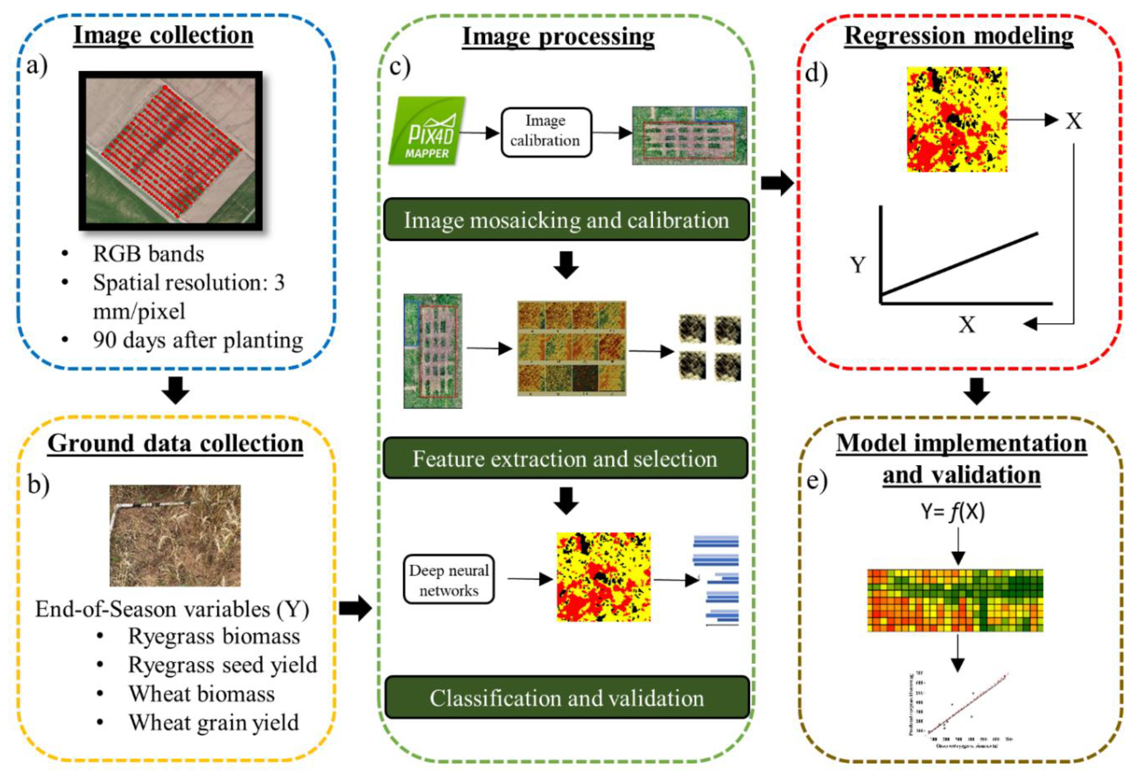
The experiment began with image collection during the early growth stage of weed, followed by an end-of-season collection of ground-truth data for both weed and crop. The next step was to process the imagery, which was conducted in three sub-steps, including image mosaicking and calibration, feature extraction and selection, and image classification and validation. Regression modelling was performed to develop predictive models using image- and ground-based information. Finally, the models were implemented on the validation plots to build a heatmap for different measured variables (Italian ryegrass biomass and seed production, and wheat biomass and grain yield reduction) and validate the accuracy of the models. Figure 2 shows the schematics of the general workflow followed in this research.

2.3. Data Collection

2.3.1. Image Collection

In order to collect early-season information required for the study, aerial flights were carried out on 6 March 2019 and 13 March 2019 at Site A and Site B, respectively. The timing coincided with the peak tillering stage of wheat and ryegrass, at about 90 DAP on both sites. A quadcopter UAV “DJI Phantom 4 Pro” (DJI, China) attached with an RGB sensor (12 megapixels) was flown at an altitude of 10 m to acquire aerial images at three different bands (Red, Green, and Blue) during ±2 h of solar noon (10 AM to 2 PM) in both sites. The average wind speed was 9.6 kmph for Site A and 8 kmph for Site B throughout the flight duration. Images were acquired at an overlapping mode (75% for both side and end overlap), the exposure was set to automatic mode, and the flight plan was executed in a grid structure at an operating speed of 5 m/s. The flight mission was executed using the mobile application “Pix4Dcapture” (Pix4D, Lausanne, Switzerland) and was completed in 20 min at each site. Reflectance panels/tarps were placed in the field at the time of flights to perform spectral calibration in the imagery at a later stage.

2.3.2. Ground-Truth Data Collection

Upon wheat maturity, ground-truth data pertaining to ryegrass biomass, ryegrass seed yield, wheat biomass, and wheat grain yield were obtained from each quadrat on 23 May 2019, to develop regression models between early-season ryegrass densities and end-of-season biophysical parameters of ryegrass and wheat. In order to account for potential ryegrass seed loss due to shattering prior to harvest, a visual estimate of seed shattering was documented at the time of harvest. The ryegrass and wheat plants were manually harvested from each quadrat at the ground level, separated by species, placed in individual paper bags, and dried in an oven at 63 °C for 36 h prior to the estimation of dry biomass. Wheat plants from each experimental unit were threshed to obtain grain yield. Ryegrass spikes were hand threshed and seed yield was determined after adjusting for shattering loss.

2.4. Image Processing

2.4.1. Image Mosaicking and Calibration

Images acquired for each site were stitched together using the Pix4D mapper software (Pix4D, Lausanne, Switzerland) to generate qualitative, high-resolution (3 mm/pixel) orthomosaic imageries. Generating qualitative orthomosaic imageries can sometimes be challenging as the process depends heavily upon several factors, including camera internal and external orientation parameters, flight parameters, and the robustness of the image-matching algorithm [32,33]. Failure to optimize the camera parameters can result in distortion of the imageries. The Pix4D mapper mitigates this issue by optimizing the camera parameters during the initial run and allowing users to re-run the process with the optimized parameters. In this study, camera model parameters were initially loaded from the exchangeable image file format metadata, generated automatically by the UAV during the image acquisition process, into the Pix4D mapper. To further improve the quality, the initial calibration phase was re-run using the optimized parameters. A detailed description of how Pix4D mapper generates an orthomosaic imagery from sets of UAV-borne imageries can be found in this link (https://support.pix4d.com/hc/en-us/articles/204272989-Offline-Getting-Started-and-Manual-pdf).
Following the orthomosaic generation, the digital number (DN) values of the imageries were calibrated to reflectance values using the three different custom spectral panels (black, grey, and white). Three different datasets, each with 300 DN or pixel values of a band as the X-variable and the reflectance values of corresponding pixels in the spectral panels derived using Analytical Spectral Devices FieldSpec Pro HandHeld spectroradiometer (Analytical Spectral Devices, Boulder, CO, USA) as the Y-variable were prepared. Furthermore, simple linear regression analyses were conducted for the X- and Y-variables to derive three separate regression models (Equations (1)–(3)) for predicting reflectance values using prepared datasets. The model was then applied to predict the values for all the pixels in red, blue, and green bands.
( σ j ) r   =   μ 1 ( λ j ) r   +   c 1
( σ j ) g = μ 2 ( λ j ) g   +   c 2  
( σ j ) b   =   μ 3 ( λ j ) b   +   c 3
where, σ j =   predicted reflectance value of a jth pixel for the red (r), green (g), and blue (b) band; λ j = DN value of a jth pixel for the red (r), green (g), and blue (b) band; μ 1, µ 2 ,   and   µ 3   are slope values derived from the linear equations for red, green, and blue band, respectively; and c1, c2, and c3 are intercepts for models for red, green, and blue band, respectively.

2.4.2. Feature Extraction and Selection

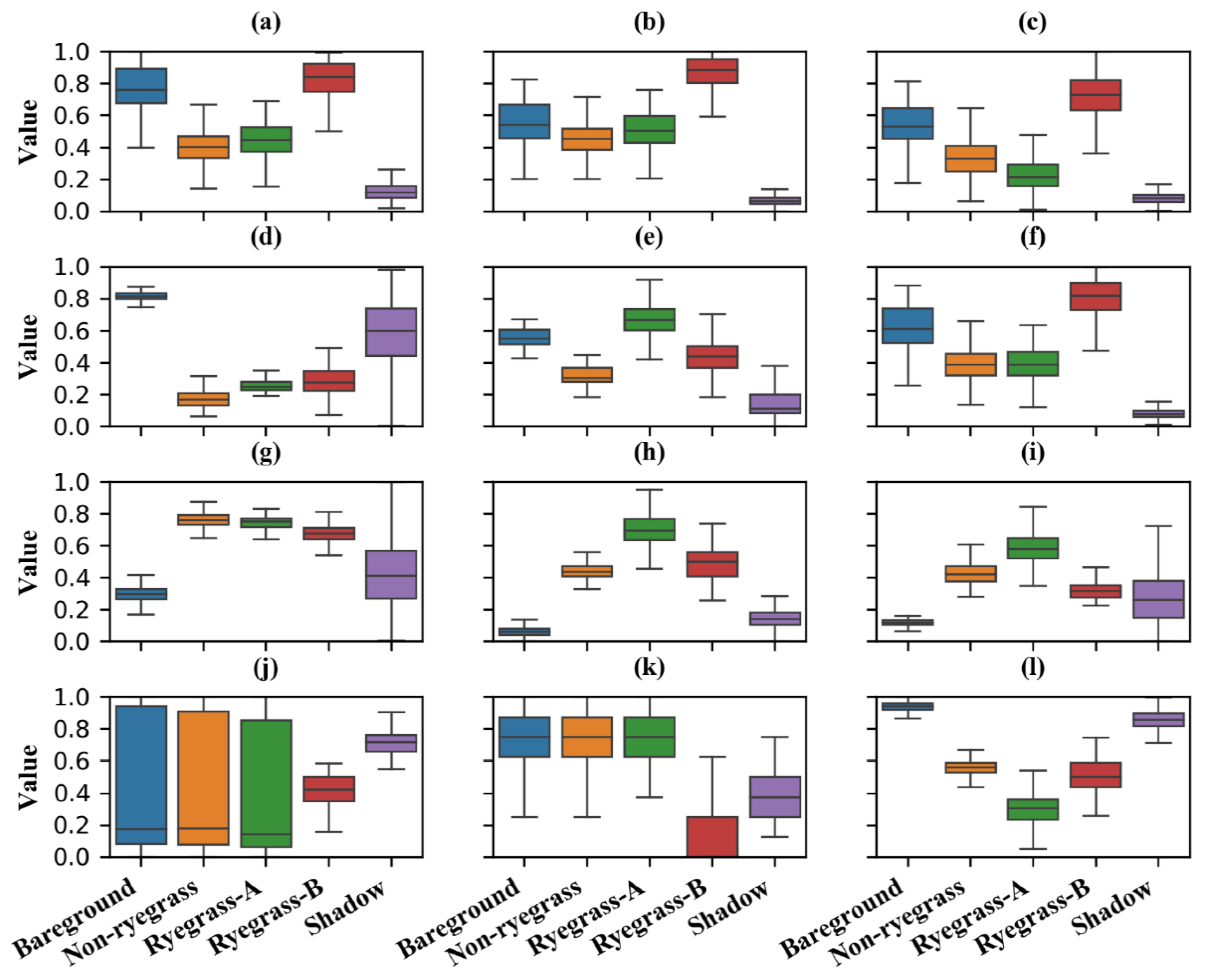
Following the spectral calibration, 12 feature layers were extracted and/or computed for further image-processing purposes (Table 1). Optimizing the feature subset is required before feeding into machine-learning algorithms for improving the classification process and making it cost- and time-efficient [34]. For this purpose, first, 1000 training samples for each of the user-defined classes (in this case, 5-classes: Ryegrass-A, Ryegrass-B, Non-ryegrass vegetation, Bareground, and Shadow) were collected from the imageries of both sites. Ryegrass-A and B represent different categories of ryegrass pixels in the imagery, indicating normal green pixels (A) and illuminated pixels (B). A considerable number of illuminated ryegrass pixels were observed in the experiment area, and the two categories were treated separately since combining them might compromise the prediction ability of the classifier. Second, the distribution of features within/across the user-defined classes were explored to select the best feature combination qualitatively. However, such a selection approach was too complex since there was much variation in the distribution of these features (Figure 3). Therefore, a wrapper-based feature selection approach called “exhaustive selection” was employed to select the 10 best feature combinations (hereafter referred to as feature models) using one-fourth of the training samples for each class (i.e., 250).

2.4.3. Image Classification and Validation

After the selection of best feature models, each feature model was tested for classifying images sampled in each quadrat (1 m × 1 m) (hereafter referred to as quadrat images) into user-defined classes using the supervised machine-learning system. The back-propagation multilayer perceptron (MLP), a commonly used and widely available ANN structure [41], was used as the machine-learning system in this study. Keras, a high-level neural networks application programming interface (API) written in python computer language [42], was used to build the MLP-based custom DNN system. Various hyperparameters were tested for several values prior to final training process to derive the best set of values (Table 2), using the same subset of training samples used for exhaustive feature selection. Categorical crossentropy was fixed for the loss function and “adam”, a very popular stochastic gradient descent-based weight optimization technique, was fixed for the optimizer in the tuning and training process.
This best set of parameters was then used in the custom DNN system to train each feature model. One-half of the training samples for each class (i.e., 500) were used for training purposes. Each trained DNN model was finally implemented over each quadrat image and in total 10 different classification outputs were generated for 10 different feature models for each image. Once the quadrat image was classified into user-defined classes, post-classification operations such as filtering, smoothing, and generalization were carried out to remove any speckled appearance and improve the quality of the classified output. For accuracy purposes, different indicators such as precision, recall, and F-score were calculated for each feature model using an independent set of validation samples [i.e., remaining one-fourth of training samples (250) for each class] and the best feature model was determined. Precision was measured as the number of correctly classified samples of a class divided by the number of samples labeled as that class by the system (Equation (4)). Recall was calculated as the number of correctly classified positive samples of a class divided by the number of validation samples allocated for that class (Equation (5)). F-score is a combination of both precision and recall (Equation (6)).
Precision   =   TP TP   +   FP
Recall   =   TP TP   +   FN
F - score   =   2   ×   Precision   ×   Recall   Precision   +   Recall
where, TP, FP, and FN represent true positive, false positive, and false negative instances, respectively.

2.5. Regression Modeling

With the classification of imageries and evaluation of the models, the best classified output, i.e., classified imagery for each quadrat (altogether 32, including both sites) were used in the regression modelling procedure. Each classified imagery comprised of pixels classified into either of the user-defined classes. First, both ryegrass classes (i.e., Ryegrass-A and B) were merged into a single class. Then, the ryegrass pixels pertaining to this class within each classified imagery were enumerated and the number of enumerated pixels was divided by total number of pixels in the imagery to calculate ryegrass canopy coverage area (%). In the next step, four separate models were developed by regressing the canopy coverage area of ryegrass (%) as the predictor variable, while considering ryegrass biomass (g), ryegrass seed yield (g), wheat biomass reduction (%), and wheat grain yield reduction (%) as predicted variables. Wheat biomass and grain yield reduction (%) were calculated as a relative measure with weed-free check plots. Altogether, 32 pairs of predicted and predictor variables (16 pairs corresponding to the quadrats for each site) were used in the regression analysis for ryegrass biomass and seed yield, whereas only 24 pairs were used for wheat biomass reduction (%) and grain yield reduction (%). Finally, the coefficient of determination (R2) and root mean square error (RMSE) were calculated as statistical measures of how well the regression predictions approximated the datapoints.

2.6. Predictive Model Implementation and Validation

The validation areas (Figure 1) were demarcated within the experimental field and the orthomosaic imageries were clipped to their extent for spatial implementation of the predictive models and independent model validation. The best feature model was also applied to the clipped imageries to obtain the classified outputs (i.e., early-season ryegrass canopy coverage maps), followed by all the post-classification operations described earlier to improve the results. The classified map was partitioned into several (1 m × 1 m) grids and the ryegrass canopy coverage area (%) was calculated for each of the grid. The predictive models developed earlier were then applied to the grids to obtain the values for all the predicted variables. Ground truth values for the 5 quadrats in each validation area pertaining to ryegrass biomass (g), ryegrass seed yield (g), wheat biomass reduction (%), and wheat grain yield reduction (%) were assessed against predicted heatmap values for those corresponding grids to determine the reliability of the whole classification and predictive model framework. RMSE and coefficient of determination (R2) were calculated as the measure of agreement between predicted and observed variables.

3. Results

3.1. Ryegrass Detection Using Feature Combinations

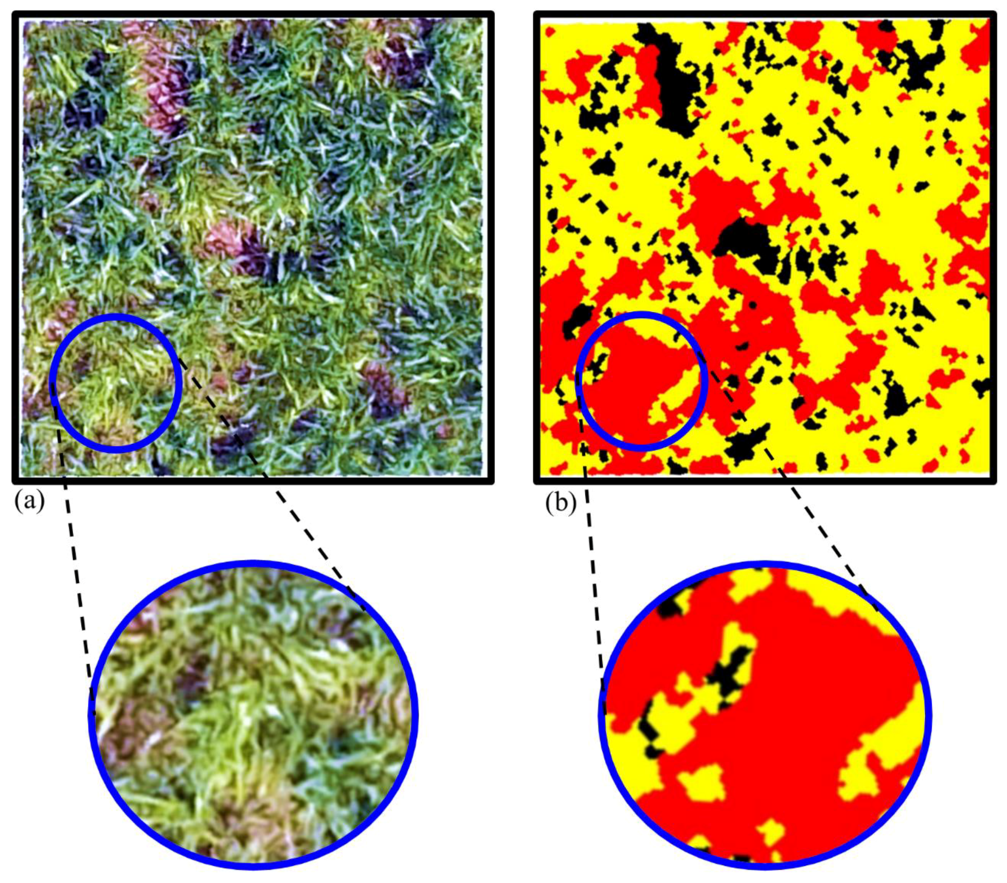
Among the approximately 4000 model runs of various features and their combinations tested in the study, the top 10 best performing models had a combination of four or more features, illustrating the robustness of multivariate analysis for species detection. Based on independent validation samples, the average F-score values ranged between 89% and 96% for different feature models (i.e., feature combinations) tested (Table 3). The highest average F-score (95.5%) was achieved with the model that combined color transformed features (hue and saturation) with vegetation indices (Excess Green Index (ExG) and Visible Atmospheric Resistant Index (VARI)) for machine learning (Model #10 in Table 3), which was closely followed by the model that used Red, Blue, Sat, VARI, ExG and Wavelet_Mean (Model #9; F-score: 95.3%). However, the model #10 was chosen for mapping Italian ryegrass (Figure 4) since it was more parsimonious compared to #9.
For model #10, the user-defined classes Bareground and Shadow were classified with the highest precision, recall and F-score (>98%), compared to the other classes namely Ryegrass-A, Ryegrass-B and Non-Ryegrass (Figure 5). As explained by boxplots for different features (Figure 3), Bareground and Shadow had very distinct boundaries from other classes for several features. The lightly shaded portion of Italian ryegrass and wheat leaves were expected to be classified as Shadow (i.e., formed underneath the canopy) due to spectral similarities; however, a meticulous training of these regions greatly reduced potential misclassification, which is indicated by the high precision (>98%) and recall (>98%) values for Shadow. The classification for Non-Ryegrass vegetation had the lowest accuracy (Figure 5; F-score: 91%), which is likely since this class encompassed a mixture of primarily wheat and few other weed species, resulting in fuzzy, instead of distinct, boundaries for different features. As a result, there could have been several instances of misclassification with either Shadow and/or Ryegrass-A. Ryegrass-B had a higher F-score (94%) compared to Ryegrass-A (92.5%) and Non-Ryegrass vegetation (91%), which could be attributed to brighter pixels of Ryegrass-B compared to the rest of the vegetation pixels, leading to distinct separation for several features. However, Ryegrass-B and Bareground overlapped for several features, as a result of reflectance from debris present on the soil surface which often produced bright reflectance.

3.2. Prediction of Competitive Outcomes between Italian Ryegrass and Wheat

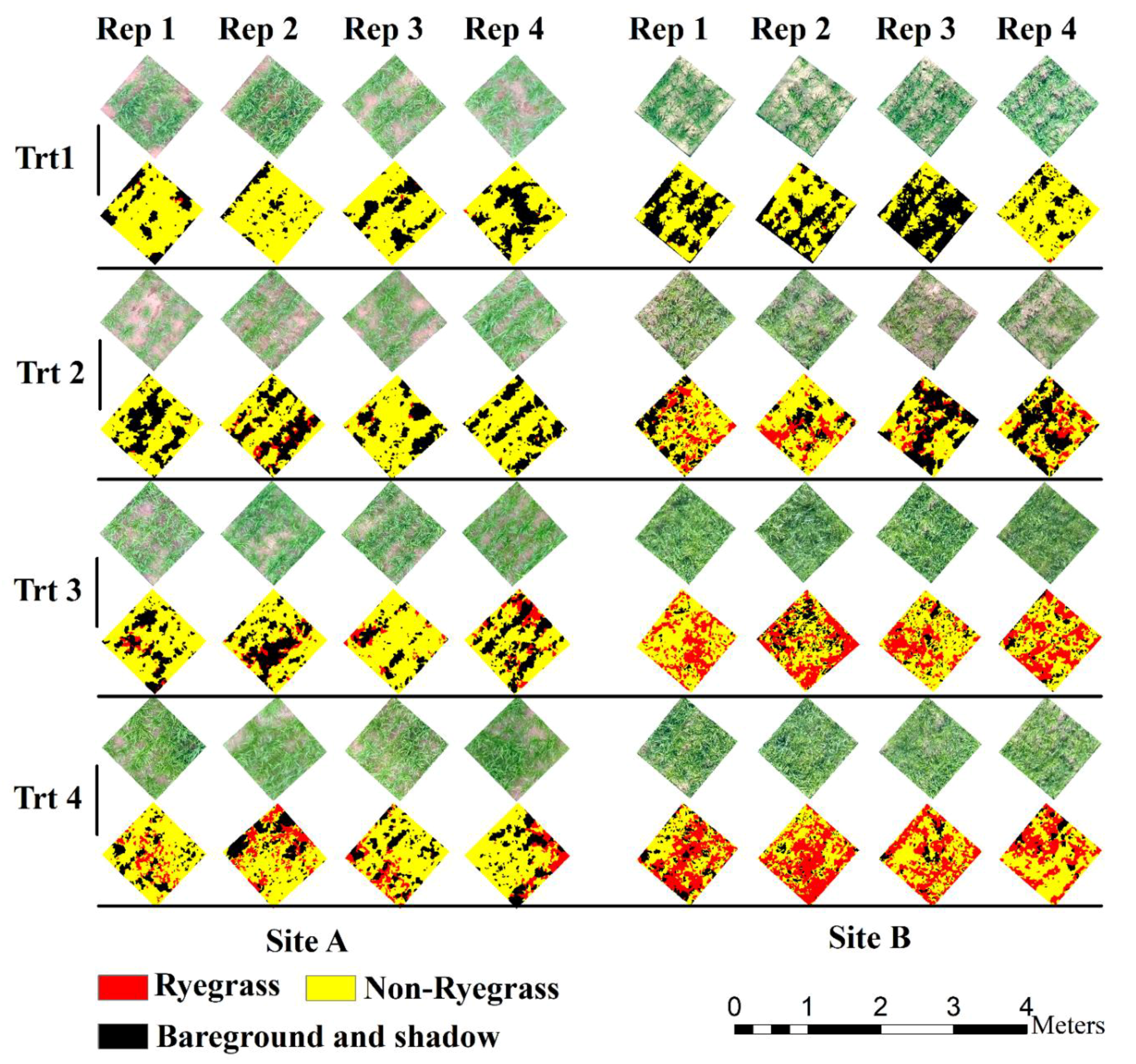
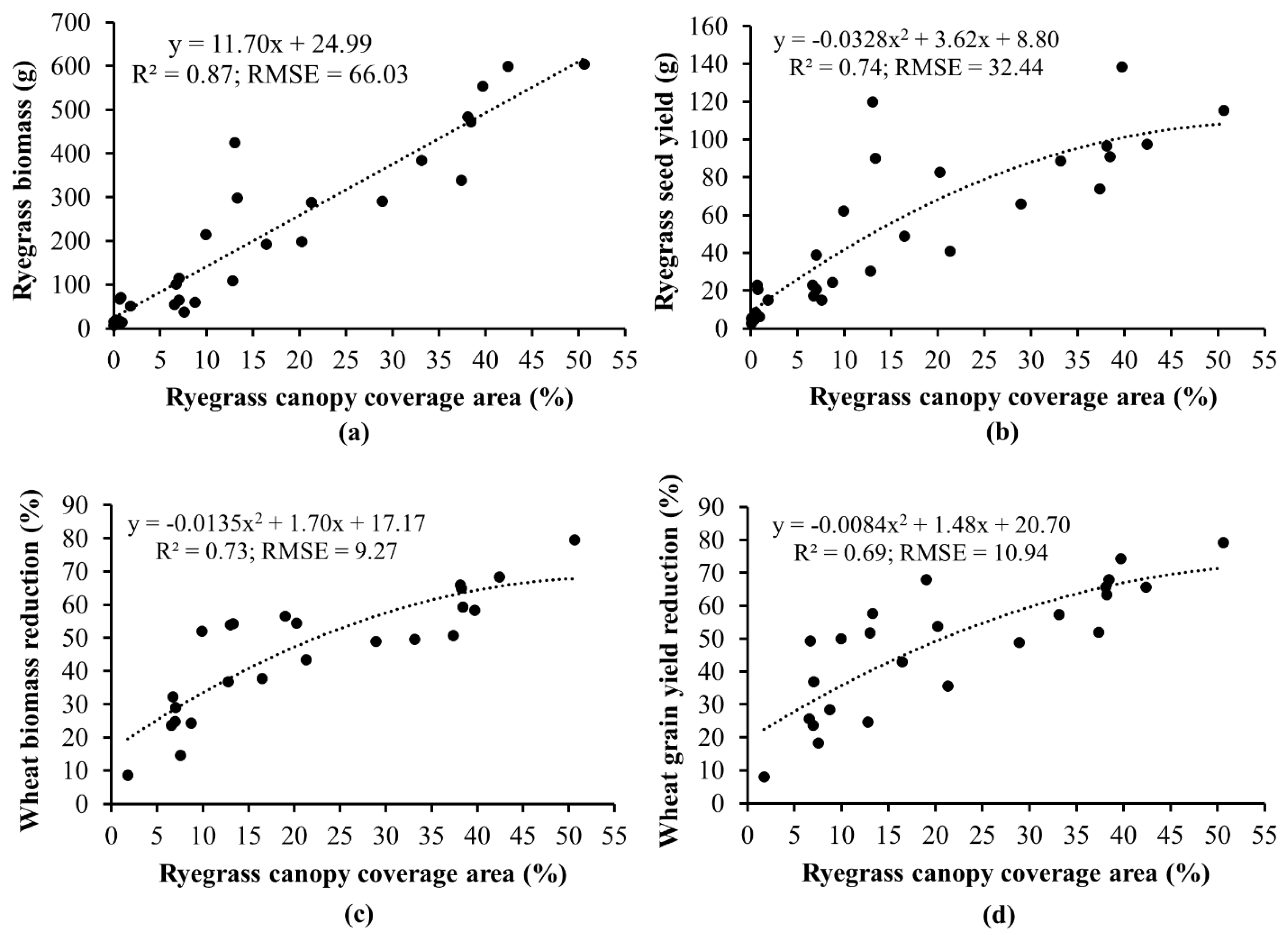
The canopy coverage area (%) for Italian ryegrass (predictor variable) was computed from each classified map of quadrat image (Figure 6) and regressed against the ground truth data (predicted variables). In general, Italian ryegrass biomass and seed production increased with an increase in their canopy coverage area (as determined through image analysis) for the densities simulated here, with a concurrent decline in wheat biomass production and grain yield. The highest coefficient of determination (R2 = 0.87; RMSE = 66.03) was achieved for prediction of ryegrass biomass, followed by ryegrass seed yield (R2 = 0.74; RMSE = 32.44), wheat biomass reduction (%) (R2 = 0.73; RMSE = 9.27), and wheat grain yield reduction (%) (R2 = 0.69; RMSE = 10.94) (Figure 7). Results showed that Italian ryegrass coverage had a linear relationship with its biomass, and a curvilinear relationship with its seed production as well as biomass and grain yield reduction of wheat.

3.3. Model Validation

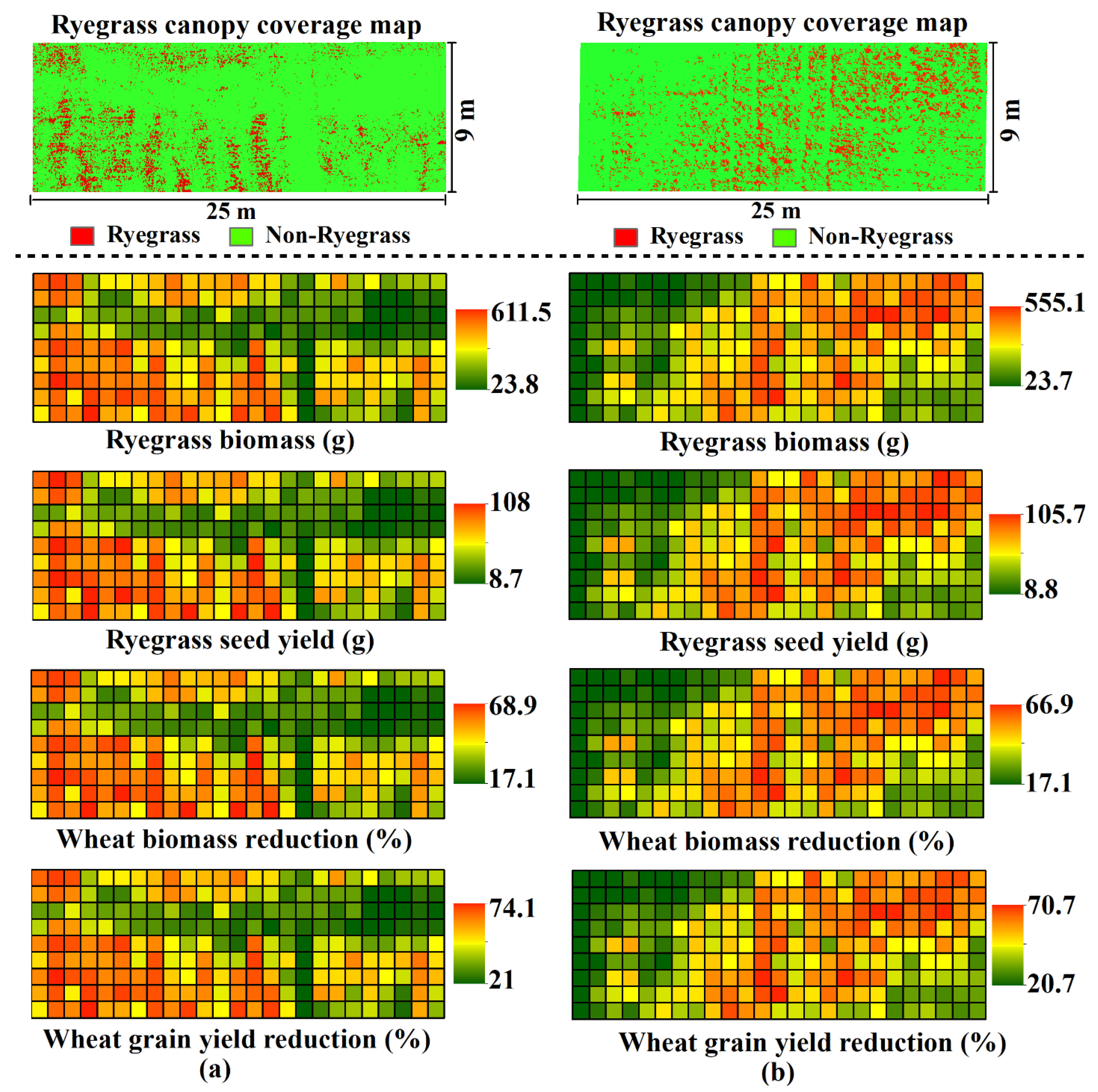
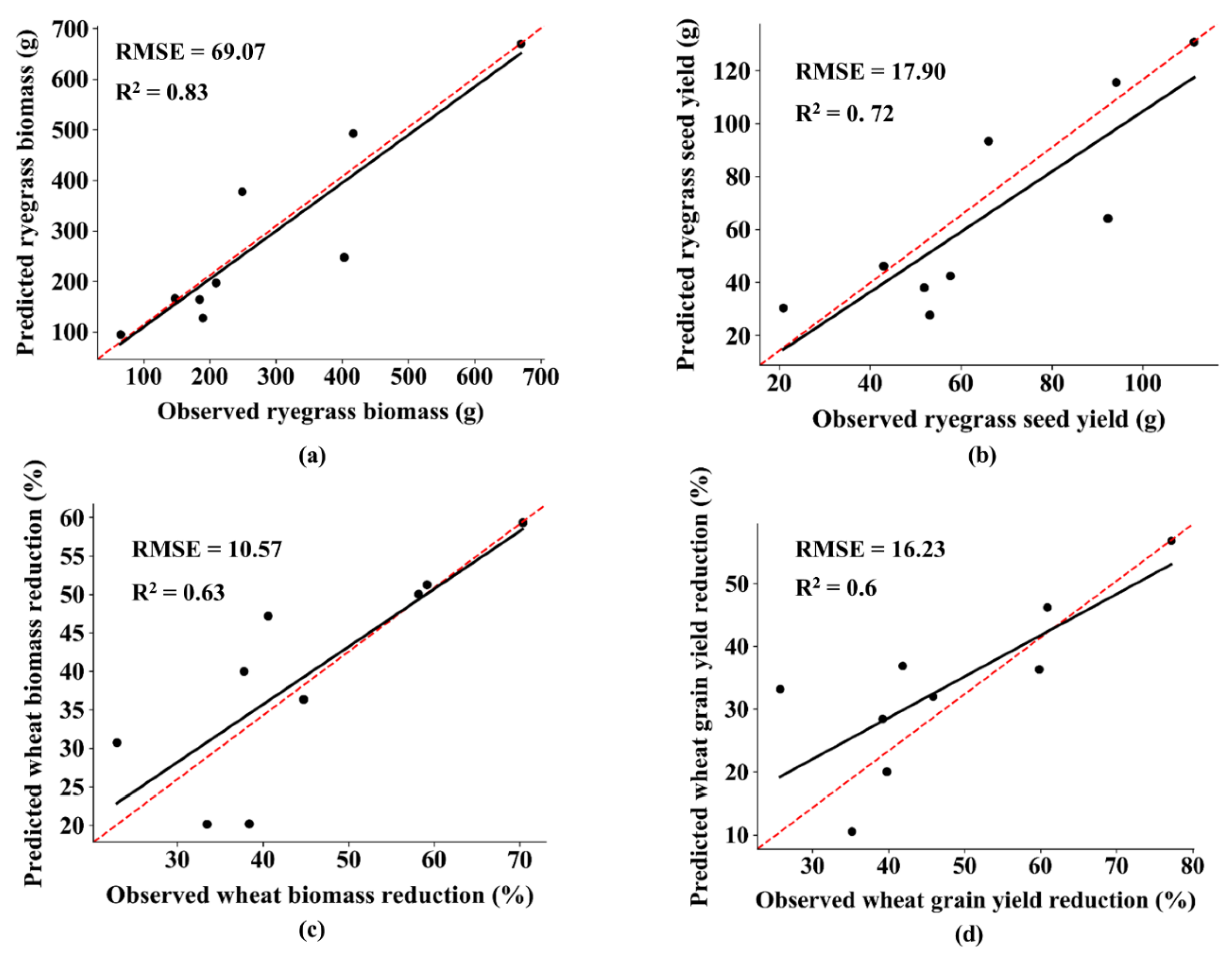
The early-season ryegrass canopy coverage maps developed with the DNN model for validation area in each site (Figure 8, top panel) and the competition models described above were utilized together to produce heat maps (1 m × 1 m grid size). These heat maps provide a visual representation of weed/crop competitive outcomes at the end of the season in terms of biomass and seed yield (Figure 8, bottom panel). Validation results showed that the coefficient of determination based on predicted (heat map-based) and observed values (ground-based) was the highest (R2 = 0.83; RMSE: 69.8) for Italian ryegrass biomass, followed by ryegrass seed yield (R2 = 0.72; RMSE = 17.9), wheat biomass reduction (%) (R2 = 0.63; RMSE: 10.57), and grain yield reduction (%) (R2 = 0.60; RMSE = 16.23) (Figure 9). Thus, the validation analysis showed that the models developed in this study were generally robust in predicting end-of-season productivity for Italian ryegrass as well as wheat.

4. Discussion

The results provide strong evidence that a combination of multiple classification features is more effective in species detection compared to employing individual features, but the choice of features is important. In this study, color-transformed features (hue and saturation) and vegetation indices (VARI and ExG) were found to be the most effective combination in detecting Italian ryegrass in wheat. Hue and saturation are invariant to brightness variation [43] and, therefore, are least affected by illumination differences by ryegrass leaves. Given the pale green color of ryegrass leaves compared to that of wheat, the difference in the greenness level was obvious with hue and saturation values. Several studies have credited hue and saturation for their ability to differentiate plants based on the greenness level [44,45]. Additionally, ExG was shown to be useful in separating plant tissues from other backgrounds (soil and weathered plant residue) [46]. VARI was designed to be minimally sensitive to atmospheric effects, allowing precise estimation of the vegetative fraction of different plant species. Recently, VARI was found to be very useful in classifying real shadows from non-sunlit plant leaves in the canopy [47]. This property of the index may have helped in reducing misclassification between shadow and non-sunlit wheat/ryegrass plant canopies in our study, as there were several non-sunlit plant pixels with shadow-like appearance in both experimental sites.
A very limited number of studies have detected/classified grass weeds in wheat using digital images (either handheld camera or UAS-derived) to date. Golzarian and Frick [14] used very high-resolution true-color images (0.26 mm/pixel) for differentiating annual ryegrass and wheat, with an accuracy of 88%. It should be noted that the current study utilized relatively lower spatial resolution (3 mm/pixel; Figure 4) and still achieved a higher accuracy (F-score: 95%). This is particularly advantageous for optimizing computational costs and complexity when scaling up this approach for vast production fields. The reasons for the improvement in classification accuracy compared to that of Golzarian and Frick [14] could be the use of DNNs, which have been proven to solve increasingly complicated applications with increasing accuracy over time [30]. However, the current study classified ryegrass at a relatively larger seedling stage compared to what was studied by Golzarian and Frick [14], which may also have affected the learning capability of the classification model.
Kodagoda et al. [13] used an overhead imaging system fitted with color and near-infrared cameras to capture high-resolution digital images in order to differentiate between wheat and two weed species, cobbler’s peg (Bidens pilosa L.) and rigid ryegrass (Lolium rigidium L.). Hue, saturation, and texture information of plant leaves were extracted from the digital images and fed into traditional machine learning algorithms such as k-means clustering and Mahalanobis distance. Although their model worked fairly well for differentiating cobbler’s peg from wheat (accuracy: 85%), it failed to detect and classify ryegrass from wheat (accuracy: 26%). Similarities of these two species in the distributions of hue, saturation, and texture cues were concluded to be the prime reason for the very low performance of the model. The current study also observed an overlap in the distribution of hue and saturation between ryegrass and non-ryegrass vegetation (Figure 3); however, supplementing with vegetation indices such as ExG and VARI was beneficial for classification.
Recently, convolutional neural networks (CNNs) have been widely appreciated for their high potential for detecting and mapping weeds [48,49,50]. However, training a CNN model for segmentation generally requires a relatively large number of annotated labels for weeds and crop canopy boundaries, making the procedure labor-intensive and time-consuming [50]. The complexity in training data preparation manifolds due to the intricate labeling procedure for grasses caused by the extreme interlocking of leaves. Moreover, this annotation process is almost impossible if the resolution of the imagery is not high enough to clearly delineate leaf boundaries. Instead of a time-consuming and intricate weed annotation procedure, this study adopted the relatively easier training sample selection approach. The most representative pixels for each user-defined class were selected as the training samples and deep neural network system was trained over the samples to achieve higher accuracy. With the intensive feature optimization technique, this study generated various feature models and tested independently to obtain the most accurate model. Feature optimization processes, such as that described in the current research, are often reported to boost machine learning performance [34].
To the best of our knowledge, very few studies have utilized DNN-based predictive models for understanding weed–crop interaction and explored the feasibility of predicting biomass and seed yield using plant canopy coverage information. Most of the existing yield prediction studies have heavily relied upon vegetation indices, especially Normalized Difference Vegetation Index (NDVI) [51,52,53]. However, several studies have reported that NDVI becomes saturated at high leaf-area index levels, which in turn may lead to inaccurate prediction of biomass and yield [54,55]. This study, in contrast, utilizes vegetation indices and other promising features to classify the pixels pertaining to the class of interest and then uses the number of pixels as the predictor variable for biomass and seed yield. Thus, this method avoids the risk of saturation and seasonal variability of vegetation indices, and leads to a better prediction.
Relatively lower correlation for wheat biomass and grain yield reduction (%) compared to ryegrass biomass and seed yield in this study could be attributed to the use of ryegrass canopy coverage area (%) as the predictor variable. In particular, wheat grain yield reduction (%) had lower coefficient of determination compared to wheat biomass because grain yield is a complex trait and is affected by several factors including environmental and genetic factors [56,57]. Although biomass has been reported to be one of the primary determinants of grain yield, other factors such as grains per spike and spikelets per plant may also have an influence [57]. Thus, the competitive effect of ryegrass on wheat grain yield may not be proportional to the effect on wheat biomass, as explained by different coefficient of determination for wheat biomass and grain yield in this study.
The ryegrass infestation map developed during the early season may help facilitate management interventions, including site-specific weed management [6]. The infestation maps can also be useful for monitoring ryegrass distribution and dynamics spatially and temporally. The predictive models and the spatial heatmap representation of weed-crop competitive interactions as presented in this study can be highly useful for management decision making [58]. Predicting weed-crop interference early-on can inform weed control thresholds required to minimize yield loss [59]. These spatial heatmaps together with weed control thresholds can be utilized to create management grids. It should also be noted that heat map representation of competitive interactions at the 1 m × 1 m grid level in this study can be scaled-up to various grid sizes to fit different management needs. Furthermore, recommendations for the features and hyperparameters made in the study could be utilized in similar studies to improve the efficiency.
This study, however, has some limitations: (1) only ANNs were tested for weed detection where several machine-learning classifiers such as random forest and support vector machine were available and already used for weed detection and mapping in the past. Future research should test these classifiers independently or maybe fused with more advanced deep-learning methods such as the CNNs; (2) broader applicability of the classification model presented here in wheat fields with varying geographies and environmental conditions is unknown. Wheat varieties may widely differ in leaf color and composition and thus may exhibit different spectral signatures. The model can be generalized and empowered with diverse training samples; (3) the competition models developed here were based solely on ryegrass canopy coverage area estimated from the aerial imageries. As such, this study did not attempt to utilize/evaluate already established weed-crop competitive models that were based on variables such as weed density [60], biomass [61,62], and leaf-area index [63]. The effectiveness of the canopy/ground cover-based prediction compared to the previously established approaches is unknown. Future research should test and ensemble these approaches to improve the accuracy and feasibility of weed–crop interaction assessments; and (4) scaling this approach to large production fields may be challenging due to high computational demands.

5. Conclusions

This study successfully identified and demonstrated a UAS-based remote-sensing approach that combined both color transformed features and vegetation indices for improved detection and mapping of Italian ryegrass in wheat (Highest F-score: 95.56 ± 4.11%). In addition, this study provided evidence that deep learning-based estimation of early-season plant canopy coverage can be a better predictor for competitive interactions, with relatively higher R2 values for developed models [0.87 for ryegrass biomass (g), 0.74 for ryegrass seed yield (g), 0.73 for wheat biomass reduction (%), and 0.69 for wheat seed yield reduction (%)]. This study also highlighted the value of affordable, computationally less complex, and less storage demanding RGB imageries in assisting farmers with weed assessment and precision weed management. The machine learning-based classification model and the weed–crop competition models developed and employed in the study will be helpful in devising suitable agronomic interventions.

Author Contributions

M.B. conceptualized, designed, and led the research; B.S. designed and conducted the study, performed data analysis, and wrote the paper; M.B., V.S., C.N., and N.R. edited and revised the paper. All authors have read and agreed to the published version of the manuscript.

Funding

This research was funded by a Texas A&M AgriLife Research Cropping Systems Seed Grant awarded to Dr. Bagavathiannan.

Conflicts of Interest

The authors declare that no conflict of interest exist.

References

  1. Tucker, K.P.; Morgan, G.D.; Senseman, S.A.; Miller, T.D.; Baumann, P.A. Identification, distribution, and control of Italian ryegrass (Lolium multiflorum) ecotypes with varying levels of sensitivity to triasulfuron in Texas. Weed Technol. 2006, 20, 745–750. [Google Scholar] [CrossRef]
  2. Stone, M.J.; Cralle, H.T.; Chandler, J.M.; Miller, T.D.; Bovey, R.W.; Carson, K.H. Above-and belowground interference of wheat (Triticum aestivum) by Italian ryegrass (Lolium multiflorum). Weed Sci. 1998, 46, 438–441. [Google Scholar] [CrossRef]
  3. Carson, K.H.; Cralle, H.T.; Chandler, J.M.; Miller, T.D.; Bovey, R.W.; Senseman, S.A.; Stone, M.J. Triticum aestivum and Lolium multiflorum interaction during drought. Weed Sci. 1999, 47, 440–445. [Google Scholar] [CrossRef]
  4. Liebl, R.; Worsham, A.D. Interference of Italian ryegrass (Lolium multiflorum) in wheat (Triticum aestivum). Weed Sci. 1987, 35, 819–823. [Google Scholar] [CrossRef]
  5. Singh, V.; Rana, A.; Bishop, M.; Filippi, A.M.; Cope, D.; Rajan, N.; Bagavathiannan, M. Chapter three-unmanned aircraft systems for precision weed detection and management: Prospects and challenges. In Advances in Agronomy; Sparks, D.L., Ed.; Academic Press: Cambridge, MA, USA, 2020; Volume 159, pp. 93–134. [Google Scholar]
  6. Thompson, J.F.; Stafford, J.V.; Miller, P.C.H. Potential for automatic weed detection and selective herbicide application. Crop Prot. 1991, 10, 254–259. [Google Scholar] [CrossRef]
  7. Mingyang, L.; Andrew, G.H.; Carol, M.-S. Characterization of multiple herbicide-resistant Italian Ryegrass [Lolium perenne L. ssp. multiflorum (Lam.)] populations from winter wheat fields in Oregon. Weed Sci. 2016, 64, 331–338. [Google Scholar]
  8. Caio, A.C.G.B.; Bradley, D.H. Multiple herbicide–resistant Italian Ryegrass [Lolium perenne L. spp. multiflorum (Lam.) Husnot] in California perennial crops: Characterization, mechanism of resistance, and chemical management. Weed Sci. 2018, 66, 696–701. [Google Scholar]
  9. Shaner, D.L.; Beckie, H.J. The future for weed control and technology. Pest Manag. Sci. 2014, 70, 1329–1339. [Google Scholar] [CrossRef] [PubMed]
  10. Ali, A.; Streibig, J.C.; Andreasen, C. Yield loss prediction models based on early estimation of weed pressure. Crop Protect. 2013, 53, 125–131. [Google Scholar] [CrossRef]
  11. López-Granados, F.; Peña-Barragán, J.M.; Jurado-Expósito, M.; Francisco-Fernández, M.; Cao, R.; Alonso-Betanzos, A.; Fontenla-Romero, O. Multispectral classification of grass weeds and wheat (Triticum durum) using linear and nonparametric functional discriminant analysis and neural networks. Weed Res. 2008, 48, 28–37. [Google Scholar] [CrossRef]
  12. Gómez-Casero, M.T.; Castillejo-González, I.L.; García-Ferrer, A.; Peña-Barragán, J.M.; Jurado-Expósito, M.; García-Torres, L.; López-Granados, F. Spectral discrimination of wild oat and canary grass in wheat fields for less herbicide application. Agron. Sustain. Dev. 2010, 30, 689–699. [Google Scholar] [CrossRef]
  13. Kodagoda, S.; Zhang, Z.; Ruiz, D.; Dissanayake, G. Weed detection and classification for autonomous farming. In Intelligent Production Machines and Systems, Proceedings of the 4th International Virtual Conference on Intelligent Production Machines and Systems, Amsterdam, The Netherlands, 3–14 July 2008; Elesevier: Amsterdam, The Netherlands, 2008. [Google Scholar]
  14. Golzarian, M.R.; Frick, R.A. Classification of images of wheat, ryegrass and brome grass species at early growth stages using principal component analysis. Plant Methods 2011, 7, 28. [Google Scholar] [CrossRef] [PubMed] [Green Version]
  15. Singh, G.; Kumar, E. Input data scale impacts on modeling output results: A review. J. Spat. Hydrol. 2017, 13, 1. [Google Scholar]
  16. Cotter, A.S.; Chaubey, I.; Costello, T.A.; Soerens, T.S.; Nelson, M.A. Water quality model output uncertainty as affected by spatial resolution of input data. J. Am. Water Res. Assoc. 2003, 39, 977–986. [Google Scholar] [CrossRef]
  17. Gao, J.; Liao, W.; Nuyttens, D.; Lootens, P.; Vangeyte, J.; Pižurica, A.; He, Y.; Pieters, J.G. Fusion of pixel and object-based features for weed mapping using unmanned aerial vehicle imagery. Int. J. Appl. Earth Obs. 2018, 67, 43–53. [Google Scholar] [CrossRef]
  18. Peña, J.M.; Torres-Sánchez, J.; de Castro, A.I.; Kelly, M.; López-Granados, F. Weed mapping in early-season maize fields using object-based analysis of unmanned aerial vehicle (UAV) images. PLoS ONE 2013, 8, e77151. [Google Scholar] [CrossRef] [Green Version]
  19. López-Granados, F.; Torres-Sánchez, J.; Serrano-Pérez, A.; de Castro, A.I.; Mesas-Carrascosa, F.J.; Peña, J.-M. Early season weed mapping in sunflower using UAV technology: Variability of herbicide treatment maps against weed thresholds. Precis. Agric. 2016, 17, 183–199. [Google Scholar] [CrossRef]
  20. Tamouridou, A.; Alexandridis, T.; Pantazi, X.; Lagopodi, A.; Kashefi, J.; Moshou, D. Evaluation of UAV imagery for mapping Silybum marianum weed patches. Int. J. Remote Sens. 2017, 38, 2246–2259. [Google Scholar] [CrossRef]
  21. De Castro, A.I.; Torres-Sánchez, J.; Peña, J.M.; Jiménez-Brenes, F.M.; Csillik, O.; López-Granados, F. An automatic random forest-OBIA algorithm for early weed mapping between and within crop rows using UAV imagery. Remote Sens. 2018, 10, 285. [Google Scholar] [CrossRef] [Green Version]
  22. Sapkota, B.; Singh, V.; Cope, D.; Valasek, J.; Bagavathiannan, M. Mapping and estimating weeds in cotton using unmanned aerial systems-borne imagery. AgriEngineering 2020, 2, 350–366. [Google Scholar] [CrossRef]
  23. Yang, M.-D.; Huang, K.-S.; Kuo, Y.-H.; Tsai, H.P.; Lin, L.-M. Spatial and spectral hybrid image classification for rice lodging assessment through UAV imagery. Remote Sens. 2017, 9, 583. [Google Scholar] [CrossRef] [Green Version]
  24. Gašparović, M.; Zrinjski, M.; Barković, Đ.; Radočaj, D. An automatic method for weed mapping in oat fields based on UAV imagery. Comput. Electron. Agric. 2020, 173, 105385. [Google Scholar] [CrossRef]
  25. Kanellopoulos, I.; Wilkinson, G.G. Strategies and best practice for neural network image classification. Int. J. Remote Sens. 1997, 18, 711–725. [Google Scholar] [CrossRef]
  26. Yang, C.C.; Prasher, S.O.; Landry, J.A.; Ramaswamy, H.S. Development of a herbicide application map using artificial neural networks and fuzzy logic. Agric. Syst. 2003, 76, 561–574. [Google Scholar] [CrossRef]
  27. Gutiérrez, P.A.; López-Granados, F.; Peña-Barragán, J.M.; Jurado-Expósito, M.; Hervás-Martínez, C. Logistic regression product-unit neural networks for mapping Ridolfia segetum infestations in sunflower crop using multitemporal remote sensed data. Comput. Electron. Agric. 2008, 64, 293–306. [Google Scholar] [CrossRef]
  28. Li, Z.; An, Q.; Ji, C. Classification of weed species using artificial neural networks based on color leaf texture feature. In Proceedings of the International Conference on Computer and Computing Technologies in Agriculture, Beijing, China, 18–20 October 2008; pp. 1217–1225. [Google Scholar]
  29. Rumelhart, D.E.; Hinton, G.E.; Williams, R.J. Learning representations by back-propagating errors. Nature 1986, 323, 533–536. [Google Scholar] [CrossRef]
  30. Goodfellow, I.; Bengio, Y.; Courville, A. Deep Learning; MIT Press: Cambridge, MA, USA, 2016. [Google Scholar]
  31. Soil Survey Staff, Natural Resources Conservation Service, United States Department of Agriculture. Web Soil Survey. Available online: http://websoilsurvey.sc.egov.usda.gov/ (accessed on 6 January 2020).
  32. Pérez, M.; Agüera, F.; Carvajal, F. Low cost surveying using an unmanned aerial vehicle. Int. Arch. Photogramm. Remote Sens. Spat. Inf. Sci 2013, 40, 311–315. [Google Scholar] [CrossRef] [Green Version]
  33. Conte, P.; Girelli, V.A.; Mandanici, E. Structure from Motion for aerial thermal imagery at city scale: Pre-processing, camera calibration, accuracy assessment. ISPRS J. Photogramm. Remote Sens. 2018, 146, 320–333. [Google Scholar] [CrossRef]
  34. Xue, B.; Zhang, M.; Browne, W.N. Particle swarm optimization for feature selection in classification: A multi-objective approach. IEEE Trans. Cybern. 2013, 43, 1656–1671. [Google Scholar] [CrossRef]
  35. Woebbecke, D.M.; Meyer, G.E.; Von Bargen, K.; Mortensen, D.A. Color indices for weed identification under various soil, residue, and lighting conditions. Trans. ASAE 1995, 38, 259–269. [Google Scholar] [CrossRef]
  36. Hunt, E.R., Jr.; Daughtry, C.S.T.; Eitel, J.U.H.; Long, D.S. Remote sensing leaf chlorophyll content using a visible band index. Agron. J. 2011, 103, 1090–1099. [Google Scholar] [CrossRef] [Green Version]
  37. Gitelson, A.A.; Kaufman, Y.J.; Stark, R.; Rundquist, D. Novel algorithms for remote estimation of vegetation fraction. Remote Sens. Environ. 2002, 80, 76–87. [Google Scholar] [CrossRef] [Green Version]
  38. Shapiro, L.; Stockman, G. Computer Vision; Prentice Hall Inc.: Upper Saddle River, NJ, USA, 2001. [Google Scholar]
  39. Stanković, R.S.; Falkowski, B.J. The Haar wavelet transform: Its status and achievements. Comput. Electron. Eng. 2003, 29, 25–44. [Google Scholar] [CrossRef]
  40. Pearson, K. On lines and planes of closest fit to systems of points in space. Lond. Edinb. Dublin Phil. Mag. J. Sci. 1901, 2, 559–572. [Google Scholar] [CrossRef] [Green Version]
  41. Atkinson, P.M.; Tatnall, A.R.L. Introduction neural networks in remote sensing. Int. J. Remote Sens. 1997, 18, 699–709. [Google Scholar] [CrossRef]
  42. Keras, F.C. The Python Deep Learning Library, 2015. Available online: https://keras.io/ (accessed on 20 September 2019).
  43. Chaves-González, J.M.; Vega-Rodríguez, M.A.; Gómez-Pulido, J.A.; Sánchez-Pérez, J.M. Detecting skin in face recognition systems: A colour spaces study. DSP 2010, 20, 806–823. [Google Scholar] [CrossRef]
  44. Hemming, J.; Rath, T. PA—Precision agriculture: Computer-vision-based weed identification under field conditions using controlled lighting. J. Agric. Eng. Res. 2001, 78, 233–243. [Google Scholar] [CrossRef] [Green Version]
  45. Burks, T.F.; Shearer, S.A.; Green, J.D.; Heath, J.R. Influence of weed maturity levels on species classification using machine vision. Weed Sci. 2002, 50, 802–811. [Google Scholar] [CrossRef]
  46. Yang, W.; Wang, S.; Zhao, X.; Zhang, J.; Feng, J. Greenness identification based on HSV decision tree. Inf. Process. Agric. 2015, 2, 149–160. [Google Scholar] [CrossRef] [Green Version]
  47. Milas, A.S.; Arend, K.; Mayer, C.; Simonson, M.A.; Mackey, S. Different colours of shadows: Classification of UAV images. Int. J. Remote Sens. 2017, 38, 3084–3100. [Google Scholar] [CrossRef]
  48. Huang, H.; Deng, J.; Lan, Y.; Yang, A.; Deng, X.; Zhang, L. A fully convolutional network for weed mapping of unmanned aerial vehicle (UAV) imagery. PLoS ONE 2018, 13, e0196302. [Google Scholar] [CrossRef] [PubMed] [Green Version]
  49. Sa, I.; Popović, M.; Khanna, R.; Chen, Z.; Lottes, P.; Liebisch, F.; Nieto, J.; Stachniss, C.; Walter, A.; Siegwart, R. WeedMap: A large-scale semantic weed mapping framework using aerial multispectral imaging and deep neural network for precision farming. Remote Sens. 2018, 10, 1423. [Google Scholar] [CrossRef] [Green Version]
  50. Gao, J.; French, A.P.; Pound, M.P.; He, Y.; Pridmore, T.P.; Pieters, J.G. Deep convolutional neural networks for image-based Convolvulus sepium detection in sugar beet fields. Plant Methods 2020, 16, 1–12. [Google Scholar] [CrossRef] [PubMed] [Green Version]
  51. Shanahan, J.F.; Schepers, J.S.; Francis, D.D.; Varvel, G.E.; Wilhelm, W.W.; Tringe, J.M.; Schlemmer, M.R.; Major, D.J. Use of remote-sensing imagery to estimate corn grain yield. Agron. J. 2001, 93, 583–589. [Google Scholar] [CrossRef] [Green Version]
  52. Xue, L.-H.; Cao, W.-X.; Yang, L.-Z. Predicting grain yield and protein content in winter wheat at different N supply levels using canopy reflectance spectra. Pedosphere 2007, 17, 646–653. [Google Scholar] [CrossRef]
  53. Zhou, X.; Zheng, H.B.; Xu, X.Q.; He, J.Y.; Ge, X.K.; Yao, X.; Cheng, T.; Zhu, Y.; Cao, W.X.; Tian, Y.C. Predicting grain yield in rice using multi-temporal vegetation indices from UAV-based multispectral and digital imagery. ISPRS J. Photogramm. Remote Sens. 2017, 130, 246–255. [Google Scholar] [CrossRef]
  54. Fassnacht, K.S.; Gower, S.T.; MacKenzie, M.D.; Nordheim, E.V.; Lillesand, T.M. Estimating the leaf area index of North Central Wisconsin forests using the landsat thematic mapper. Remote Sens. Environ. 1997, 61, 229–245. [Google Scholar] [CrossRef]
  55. Turner, D.P.; Cohen, W.B.; Kennedy, R.E.; Fassnacht, K.S.; Briggs, J.M. Relationships between leaf area index and landsat TM spectral vegetation indices across three temperate zone sites. Remote Sens. Environ. 1999, 70, 52–68. [Google Scholar] [CrossRef]
  56. Yagbasanlar, T.; Özkan, H.; Genç, I. Relationships of growth periods, harvest index and grain yield in common wheat under Mediterranean climatic conditions. Cereal Res. Commun. 1995, 23, 59–62. [Google Scholar]
  57. Slafer, G.; Calderini, D.; Miralles, D. Yield components and compensation in wheat: Opportunities for further increasing yield potential. In Increasing Yield Potential in Wheat: Breaking the Barriers; Reynolds, M.P., Rajaram, S., McNab, A., Eds.; CIMMYT: El Batan, Mexico, 1996; pp. 101–133. [Google Scholar]
  58. Heather, J.G.; Bennett, K.A.; Ralph, B.B.; Tardif, F.J. Evaluation of site-specific weed management using a direct-injection sprayer. Weed Sci. 2001, 49, 359–366. [Google Scholar]
  59. Swanton, C.J.; Weaver, S.; Cowan, P.; Acker, R.V.; Deen, W.; Shrestha, A. Weed thresholds. J. Crop Prod. 1999, 2, 9–29. [Google Scholar] [CrossRef]
  60. Cousens, R. A simple model relating yield loss to weed density. Ann. Appl. Biol. 1985, 107, 239–252. [Google Scholar] [CrossRef]
  61. Christensen, S. Crop weed competition and herbicide performance in cereal species and varieties. Weed Res. 1994, 34, 29–36. [Google Scholar] [CrossRef]
  62. Colbach, N.; Collard, A.; Guyot, S.H.M.; Meziere, D.; Munier-Jolain, N. Assessing innovative sowing patterns for integrated weed management with a 3D crop:weed competition model. Eur. J. Agron. 2014, 53, 74–89. [Google Scholar] [CrossRef]
  63. Kropff, M.J.; Spitters, J.T. A simple model of crop loss by weed competition from early observations on relative leaf area of the weeds. Weed Res. 1991, 31, 97–105. [Google Scholar] [CrossRef]
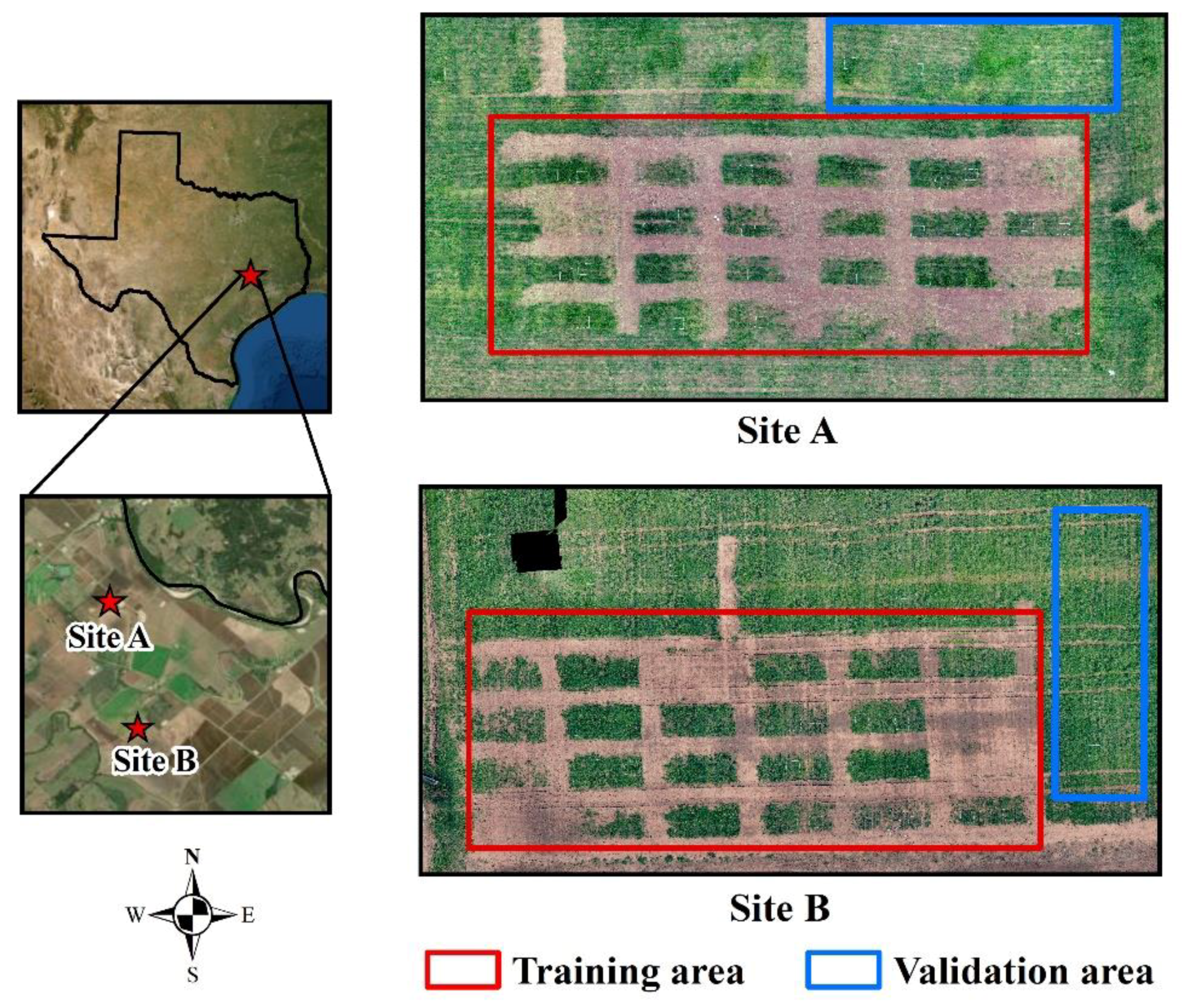
Figure 1. Study locations (Burleson county, Texas, U.S.) and experimental setup for detecting Italian ryegrass and evaluating the competitive response with wheat using unmanned aerial vehicle (UAV)-based aerial true color imagery (spatial resolution 3 mm/pixel). The study locations are located approximately 4 km apart and are unique in edaphic characteristics. Training area includes all the experimental units that would be used for building predictive models and validation area includes the area that would be subjected to validate the accuracy of the model.
Remotesensing 12 02977 g001
Figure 2. Flowchart for the overall methodology followed in this research for detecting Italian ryegrass in wheat and prediction of competitive interactions. The specific steps included (shown in dashed boxes) are: (a) image collection, (b) ground data collection, (c) image processing, (d) regression modeling, (e) model implementation and validation.
Remotesensing 12 02977 g002
Figure 3. Boxplots showing the distribution of features for each of the user-defined classes, with X- and Y-axis being the user-defined classes and corresponding normalized values, respectively. The colored portion of boxplots shows inter-quartile range of the red band (a), green band (b), blue band (c), hue (d), saturation (e), value (f), Visible Atmospheric Resistant Index (g), Triangular Greenness Index (h), Excess Greenness Index (i), wavelet transformed coefficients mean (j), wavelet transformed coefficients standard deviation (k), and principal component 1 (l).
Remotesensing 12 02977 g003
Figure 4. An example imagery showing Italian ryegrass coverage in wheat in a moderate density experimental unit (i.e., 1 m × 1 m quadrat) established in this study (a) and its corresponding classified map (b). The imagery for the experimental unit was classified using the best feature model determined in the study. The zoomed circles beneath the panels a and b represent a specific section of the imagery and its corresponding map. The red, yellow, and black colors in the map represent ryegrass coverage area, non-ryegrass vegetation, and baregound and shadow areas, respectively.
Remotesensing 12 02977 g004
Figure 5. Accuracy statistics for the best model used for detecting Italian ryegrass in wheat, which combined color transformed features with vegetation indices. Precision, recall, and F-score values (%) (Y-axis) are shown for each of the five user defined classes (X-axis).
Remotesensing 12 02977 g005
Figure 6. Implementation of the best model, that utilized color transformed features and vegetation indices, over training experimental units (1 m × 1 m quadrats) in both study sites (A and B) to detect and map Italian ryegrass in wheat. The figure consists of true color imagery and corresponding classified maps for the experimental units for weed-free check (Trt 1), low (Trt 2), moderate (Trt 3), and high (Trt 4) density treatments (red pixels: Italian ryegrass; yellow pixels: vegetation other than Italian ryegrass; and black pixels: bareground and shadow). Abbreviations: trt-treatments; rep-replications. Note: since each experimental unit was clipped based on the quadrat’s boundary visible in the imagery and because the imagery was not perfectly ortho-rectified, the size of the clipped units may range between 1 ± 0.05 m. However, this may not affect the analysis as ryegrass canopy coverage (%) was calculated based on the total size of the unit.
Remotesensing 12 02977 g006
Figure 7. Regression analysis between Italian ryegrass canopy coverage area (%) determined using image analysis and ground truth Italian ryegrass biomass (a), Italian ryegrass seed yield (b), wheat biomass reduction (%) (c), and wheat grain yield reduction (%) (d). The canopy coverage area (%) was derived from the classified images for experimental units (1 m × 1 m), whereas predicted variables (y-variables) were ground/field-based data.
Remotesensing 12 02977 g007
Figure 8. Implementation of predictive models over two validation sites (a,b). Predictions were done on 1 m × 1 m spatial grids created over the ryegrass canopy coverage map developed during early season (layers above the dashed line in the figure). The maps below the dashed line show the gradient of model predicted end-of-season estimates for different variables in each 1 m × 1 m grid.
Remotesensing 12 02977 g008
Figure 9. Predicted vs observed values in the validation experiment for different competition models pertaining to Italian ryegrass biomass (a), Italian ryegrass seed yield (b), wheat biomass reduction (%) (c), and wheat grain yield reduction (%) (d). The red-dashed line represents 1:1 slope line or reference diagonal line (expected values) and the black solid line represents the observed slope line between the predicted and observed datasets. The units of root mean square error (RMSE) values correspond to the units of respective predictor/observed values.
Remotesensing 12 02977 g009
Table 1. Details of various features extracted and/or computed for image classification, through several computational procedures on the pixel value of imageries. The value in parenthesis indicates number of features belonging to the feature category.
CategoryFeaturesDescription/Formula **Reference
Original bands (3)Blue --
Green
Red
Vegetation indices (3)Excess Green Index (ExG) 2 ×   G     R     B R   +   G   +   B [35]
Triangular Greenness Index (TGI)   190   ( R     G )     120 ( R     B ) 2 [36]
Visible Atmospheric Resistant Index (VARI) G     R G   +   R     B [37]
Color space transformed features (3)Hue A gradation or variety of a color [38]
SaturationDepth, purity, or shades of the color
ValueBrightness intensity of the color tone
Wavelet transformed coefficients (2)Wavelet coefficient meanMean value calculated for a pixel using discrete wavelet transformation[39]
Wavelet coefficient standard deviationStandard deviation calculated for a pixel using discrete wavelet transformation
Principal components (1)Principal component 1Principal component analysis-derived component accounting maximum amount of variance [40]
** Abbreviations: R, G, and B represent Red, Green, and Blue bands, respectively.
Table 2. Various hyperparameters and several potential values for corresponding hyperparameters tested for the best performance of the custom deep neural network system using the grid search cross validation method. A total of 150 trials were conducted to obtain the best set of values.
HyperparameterValuesSelected Value(s)
Number of hidden layers1,2,3,4,55
Nodes in hidden layers *(20)
(40, 20)
(60, 40, 20)
(80, 60, 40, 20)
(100, 80, 60, 40, 20)
(100, 80, 60, 40, 20)
Activation function“Rectified linear unit”
“Sigmoid function”
“Rectified linear unit”
Batch size10, 20, 30, 40, 5020
Number of epochs100, 300, 500100
* The values for hyperparameter “nodes in hidden layers” were assigned with respect to “number of hidden layers”.
Table 3. Validation samples-based accuracy statistics for 10 best feature models used for detecting Italian ryegrass in wheat. The 10 best feature models were determined through the exhaustive feature selection process. The accuracy statistics for each feature model were based on 250 samples for each user-defined class.
Feature Model #Features Used **Precision (%) *Recall (%) *F-score (%) *
1Green, Blue, Hue, Sat, Value, TGI, ExG, PC-194.28 ± 4.8694.28 ± 5.2494.27 ± 4.96
2Hue, Value, VARI, ExG94.28 ± 4.5094.28 ± 7.9494.27 ± 5.26
3Red, Hue, Sat, VARI, ExG, Wavelet_Mean94.95 ± 4.5894.91 ± 4.9894.91 ± 4.43
4Hue, VARI, TGI, ExG91.53 ± 6.7590.63 + 8.9390.54 + 2.29
5Green, Blue, Hue, Sat, Value, ExG, Wavelet_Mean, PC-195.33 ± 4.2395.38 ± 5.0795.36 ± 4.14
6Red, Green, Hue, Sat, ExG, Wavelet_Std94.45 ± 4.6794.44 ± 5.8394.41 ± 4.98
7Red, Green, Hue, Sat, TGI, Wavelet_Std95.01 ± 4.3194.94 ± 5.594.91 ± 4.25
8Sat, Value, VARI, ExG91.74 ± 8.1491.59 ± 9.4891.54 ± 8.21
9Red, Blue, Sat, VARI, ExG, Wavelet_Mean95.01 ± 4.7194.97 ± 5.3694.96 ± 4.67
10Hue, Sat, VARI, ExG95.34 ± 4.2795.68 ± 5.0595.56 ± 4.11
* A single mean value calculated by averaging the values of all the user-defined classes, and standard deviation value calculated among the accuracies for each user-defined class for each feature model.
** Abbreviations: ExG-Excess Greenness Index, PC-Principal component, Sat-Saturation, TGI-Triangular Greenness Index, VARI-Visible Atmospheric Resistant Index, Wavelet_mean-Wavelet transformed coefficient mean value, Wavelet_std-Standard deviation of Wavelet transformed coefficients mean value.