Article

Mapping Crop Types in Southeast India with Smartphone Crowdsourcing and Deep Learning

1
Institute for Computational and Mathematical Engineering, Stanford University, Stanford, CA 94305, USA
2
Department of Earth System Science and Center on Food Security and the Environment, Stanford University, Stanford, CA 94305, USA
3
Progressive Environmental & Agricultural Technologies, 10435 Berlin, Germany
*
Author to whom correspondence should be addressed.
Remote Sens. 2020, 12(18), 2957; https://doi.org/10.3390/rs12182957
Submission received: 25 July 2020 / Revised: 26 August 2020 / Accepted: 5 September 2020 / Published: 11 September 2020
(This article belongs to the Section Remote Sensing in Agriculture and Vegetation)

Abstract

:
High resolution satellite imagery and modern machine learning methods hold the potential to fill existing data gaps in where crops are grown around the world at a sub-field level. However, high resolution crop type maps have remained challenging to create in developing regions due to a lack of ground truth labels for model development. In this work, we explore the use of crowdsourced data, Sentinel-2 and DigitalGlobe imagery, and convolutional neural networks (CNNs) for crop type mapping in India. Plantix, a free app that uses image recognition to help farmers diagnose crop diseases, logged 9 million geolocated photos from 2017–2019 in India, 2 million of which are in the states of Andhra Pradesh and Telangana in India. Crop type labels based on farmer-submitted images were added by domain experts and deep CNNs. The resulting dataset of crop type at coordinates is high in volume, but also high in noise due to location inaccuracies, submissions from out-of-field, and labeling errors. We employed a number of steps to clean the dataset, which included training a CNN on very high resolution DigitalGlobe imagery to filter for points that are within a crop field. With this cleaned dataset, we extracted Sentinel time series at each point and trained another CNN to predict the crop type at each pixel. When evaluated on the highest quality subset of crowdsourced data, the CNN distinguishes rice, cotton, and “other” crops with 74% accuracy in a 3-way classification and outperforms a random forest trained on harmonic regression features. Furthermore, model performance remains stable when low quality points are introduced into the training set. Our results illustrate the potential of non-traditional, high-volume/high-noise datasets for crop type mapping, some improvements that neural networks can achieve over random forests, and the robustness of such methods against moderate levels of training set noise. Lastly, we caution that obstacles like the lack of good Sentinel-2 cloud mask, imperfect mobile device location accuracy, and preservation of privacy while improving data access will need to be addressed before crowdsourcing can widely and reliably be used to map crops in smallholder systems.

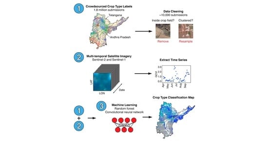
Graphical Abstract

1. Introduction

Smallholder farms—commonly defined as holdings smaller than 2 ha in size [1]—make up 84% of the world’s 570 million farms [2], provide a living for two-thirds of the world’s 3 billion rural population [3], and produce an estimated one-third of global food consumed [4,5]. In the developing nations of Asia and Africa, smallholder agriculture is vital to achieving food security under growing populations [3]. Relative to this global significance, there is a scarcity of data on smallholder crop production, starting at the fundamental questions of which crop types smallholders grow and where they grow them. Both pieces of information are needed to track smallholder yield progress, study management strategies, and design targeted agricultural policies [6,7]. The data gap exists because most smallholders are located in countries where infrastructure to conduct surveys—the traditional way of obtaining farm-level information—is still nascent or under development [8]. Where official statistics on crop area and production do exist, they are aggregated to regional or national levels [9], or, in the case of the World Bank’s Living Standards Measurement Study, available for a random sample of a country’s villages [10].
Remote sensing data offers a low-cost, large-scale, and continuously-updated supplement to surveys [11]. In the past decade, advances in the resolution of satellite sensors, data storage and processing, and machine learning algorithms have enabled the development of annual crop type maps in the United States [12], Canada [13], and Europe [14] at sub-field levels. They have the potential to do the same in areas dominated by smallholder agriculture, if two main challenges can be overcome. First, field-level ground data are still required to train, or at least validate, models that can relate remote sensing data to crop types. As mentioned, many countries lack the infrastructure to conduct surveys to obtain these ground truth labels at a national scale. Second, smallholder systems are more heterogeneous than the industrial agriculture that dominates North America and Europe, where most crop type mapping methods have focused to date. Fields are smaller, on-farm species are more diverse, management practices are more variable, and intercropping and multi-crop rotations are common [2,15,16]. These attributes complicate the use of moderate-resolution satellite imagery and increase variability within the same field, making it difficult to distinguish crop types from each other.
Without publicly-available, government-led field surveys, researchers have either organized their own surveys [14,17,18,19] or mobilized citizen science efforts [20,21] to obtain ground truth labels in smallholder systems. Most often, these labels are used in conjunction with supervised machine learning methods [14,17,18,19,21] or classification rules designed by crop experts [22,23]. These approaches have shown that supervised machine learning methods like random forests can achieve some success discerning crop types in smallholder systems, but small field size, high within-crop variation, and low training set size continue to limit map accuracies and the generalizability of models. In works where no field-level ground truth is available [24,25], maps have been validated against sub-national production statistics, but their field-level accuracies are unknown.
In India, no national field-level crop type map exists for public use at the time of writing. Large-scale crop type mapping efforts have mostly focused on rice (paddy), which covers the most cultivable land in India [9] and has a distinct spectral time series due to periodic flooding of fields. Examples of rice maps include moderate-resolution MODIS- or SPOT-based maps across South Asia [24,26,27] and a 10 m-resolution Sentinel-1-based map in northeast India [21]. Due to the small size of Indian crop fields [28], only the latter can be considered field-level mapping. Maps of wheat [19,29] and sugarcane [30,31] have also been created at local scales, illustrating the potential of remote sensing-based crop mapping across India’s diverse agricultural landscape. However, to create national or state-wide multi-crop maps and validate them against field observations requires expansive ground truth datasets that have thus far been unavailable.
In this study, we demonstrate the use of crowdsourced ground data, high resolution Sentinel and DigitalGlobe satellite imagery, and neural networks to map kharif rice and cotton at 10 m resolution in southeast India. To fill the gap in field-level crop labels, we used over 1.8 million geotagged submissions from local farmers to Plantix, a free Android application that uses image recognition to diagnose crop diseases and classify crop types. The high volume of data was possible because, unlike previous efforts at crowdsourcing crop labels that enlisted researchers and volunteers [20,21], Plantix offers farmers a service at a time when 18% of rural India has access to mobile internet [32]. With high data volume, however, comes high levels of noise and sampling bias not present in well-designed surveys. To render the Plantix data usable, we filtered and resampled the submissions to 10,000 geographically representative points spanning the major monsoon-season crops—a dataset comparable in size to the ground truth collected by Indian state agriculture departments annually (11,469 points nationally in kharif and rabi from 2017–2018) [33].
Next, to address the second challenge of classifying crop types in a heterogeneous landscape with very small fields, we used multi-temporal radar (Sentinel-1) and optical (Sentinel-2) images at 10 m resolution, augmented with very high resolution (0.3 m) static DigitalGlobe images to ensure that labeled Sentinel pixels are within a crop field. We compared classification using Fourier transform coefficients [34,35,36] and random forests [37] with classification using raw time series input to convolutional neural networks [38]. We tested whether classification was robust to moderate amounts of training set and validation set noise, and validated model predictions against both a hold-out set of farmer submissions and sub-national crop area statistics. Our final crop type map covers rice and cotton at 10 m resolution across Andhra Pradesh and Telangana for the 2018 kharif season.

2. Study Region

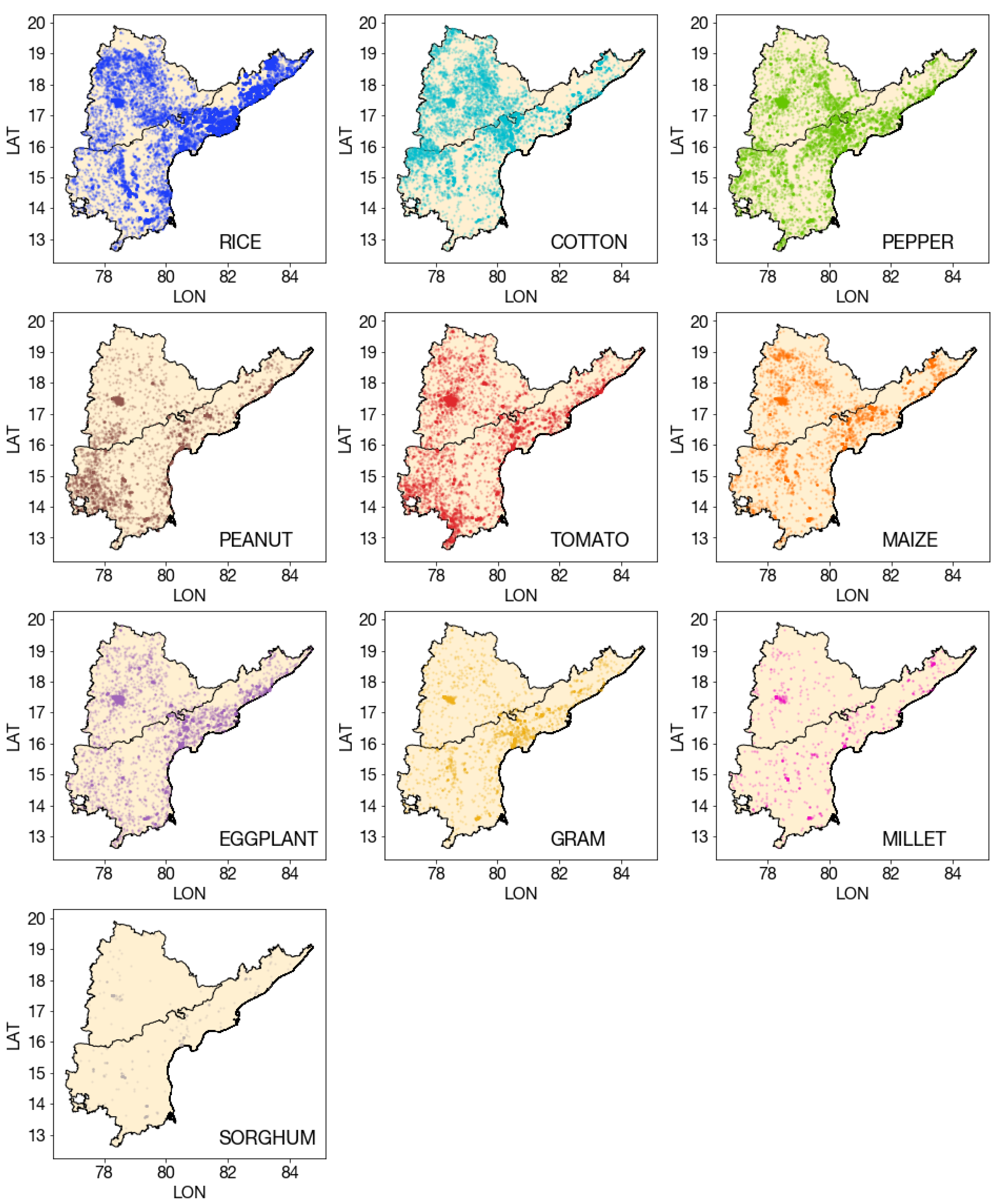
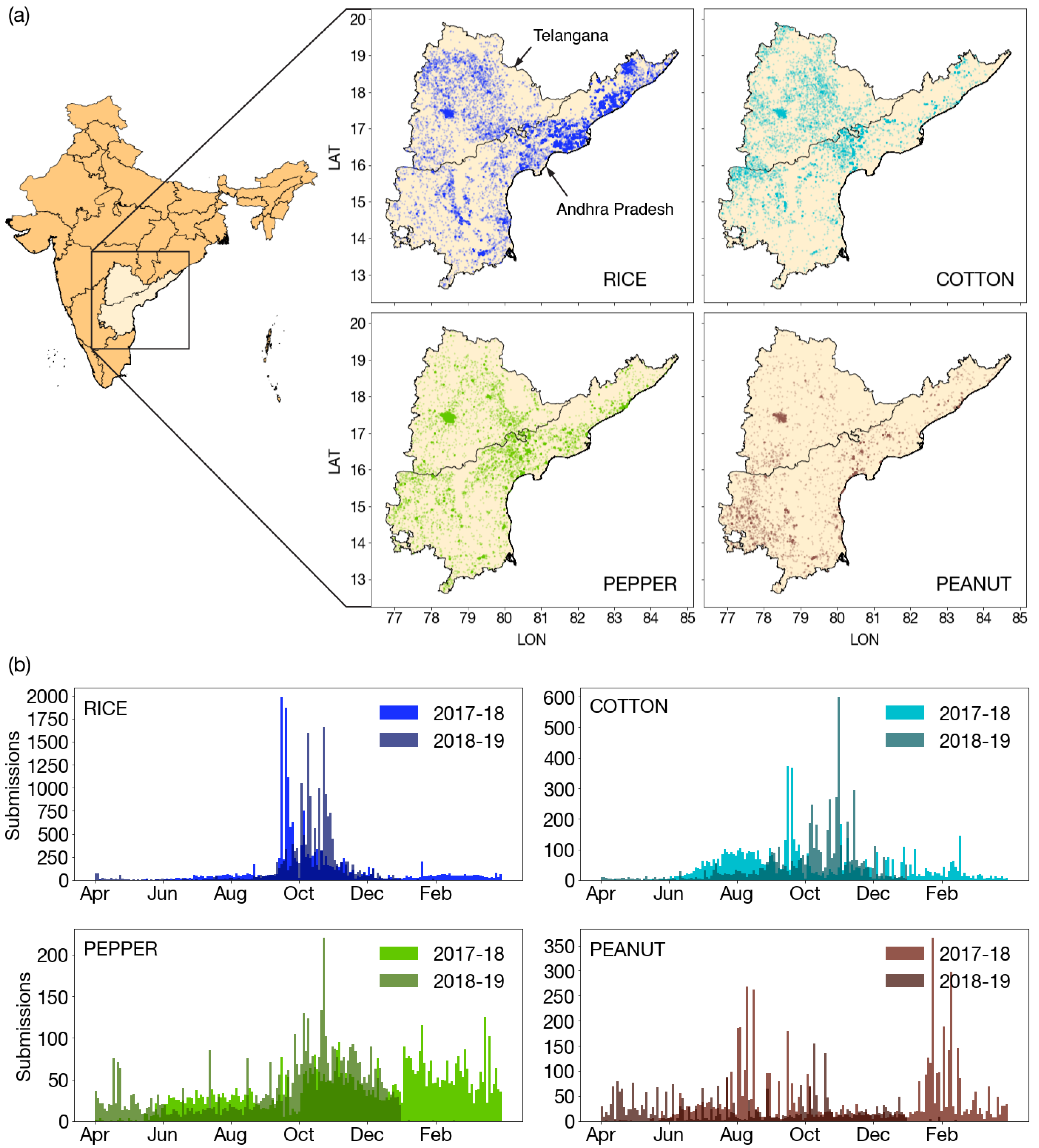
India is comprised of 29 states, whose climates range from tropical in the south to arid in the northwest and support a large diversity of crop types. In this study, we focus on developing crop type mapping methodology in two states: Andhra Pradesh and Telangana, where the Plantix app received the largest number of user submissions between 2017 and 2019 (Figure 1).
Andhra Pradesh (AP) lies on the southeastern coast of India, bordering the Bay of Bengal. It is the seventh largest Indian state (160,200 sq km) and accounts for 7.3 % of the country’s total irrigation [39]. The state is dominated by a semi-arid tropical climate; districts experience annual rainfalls of 700 mm to 1200 mm falling mostly within July to October and temperatures varying from 15  C to 45  C [40]. In 2014, the Ministry of Agriculture reported that 40 % of the state is cropped, while another 22 % is forest [40]. Like much of India, AP has two main cropping seasons: kharif, from June to November coinciding with the southwest monsoon, and rabi, from November to May in drier months and requiring irrigation. Rice (paddy), cotton, and peanut (groundnut) account for over 70 % of cropped area in the kharif season, while rice, chickpea (gram), and black gram (urad) dominate the rabi season [9]. The 2015–2016 Indian Agriculture Census revealed that the average operational holding size in AP was 0.94 ha [28].
Telangana borders Andhra Pradesh to the northwest, and until 2014 was part of Andhra Pradesh. Today it is the eleventh largest Indian state (112,077 sq km). Situated on the Deccan Plateau in central-south India, its climate is semi-arid and drier than that of AP, with district average annual precipitation more variable from 500 mm to 1200 mm and temperatures from 15 °C to 45 C. Forty-three percent of the state is cropped, and  24 % is forest [40]; cotton, rice, and maize are major kharif crops, while rice, maize, and peanut comprise the major rabi crops [9]. The average operational holding size in Telangana was 1.00 ha in 2015–2016 [28].

3. Datasets

3.1. Plantix User Submissions

Plantix is a free Android application created by Progressive Environmental and Agricultural Technologies (PEAT) in 2015 to help farmers identify pests, diseases, and nutrient deficiencies using a mobile phone camera and image recognition software. The user—usually a farmer, sometimes a hired plant expert—takes a photo of his or her crop with a mobile phone and uploads the photo to PEAT servers for a diagnosis of plant health. The photo is then run through a deep neural network, which returns predicted plant ailments. This information, along with corresponding treatments, are sent back to the user’s Plantix app.
Between 1 January 2017 and 1 January 2019, the Plantix app received 8.6 million geolocated submissions from India, 1.8 million of which were in Andhra Pradesh and Telangana. When a photo was taken via Plantix, the time of capture and the location of the phone were recorded. Figure 1 shows that most of the submissions were logged between September and November, which is during the harvest of the kharif season. While submissions were not tagged with a crop type by the farmer, crop scientists at PEAT assigned a crop type label to a subset of the submissions based on the uploaded photos, and a deep convolutional neural network (Plantix-DNN) was trained on expert labels to predict the crop type of all million submissions.
Details of how Plantix submissions were filtered and used to construct training, validation, and test sets for crop type classification are described in Section 4.1.

3.2. Sentinel-2 Time Series

Sentinel-2 was chosen for its high spatial resolution and public availability, and prior work has shown that optical features can be used to distinguish crop types [14,18,27,41]. Sentinel-2A was first launched by the European Space Agency (ESA) in June 2015 as part of the European Union’s Copernicus Programme for Earth observation, and captures high-resolution (10–60 m) optical imagery to serve a wide range of scientific applications on land and in coastal waters. Since March 2017, with the launch of Sentinel-2B, images have been collected on a 5-day cycle. ESA distributes a top of atmosphere reflectance product (Level-1C) for Sentinel-2, while a higher-level surface reflectance product (Level-2A) can be derived using a toolbox provided by ESA [42]. At the time of this work, pre-generated Level-2A imagery was not available for download from either ESA or Google Earth Engine (GEE) over India before December 2018. Since the ESA Toolbox was also not available in GEE, one would have to compute the Level-2A product and ingest it into GEE in order to obtain time series of surface reflectance. Such an approach is hugely expensive computationally and storage-wise, and does not scale well to a study region as large as Andhra Pradesh and Telangana. Furthermore, prior work showed that land cover classification using top-of-atmosphere reflectance is comparable to using surface reflectance, since relative spectral differences drive classification [43,44]. For these reasons, we used the Level-1C product, with the recognition that this imperfect input will still place some limits on the performance of a crop classifier.
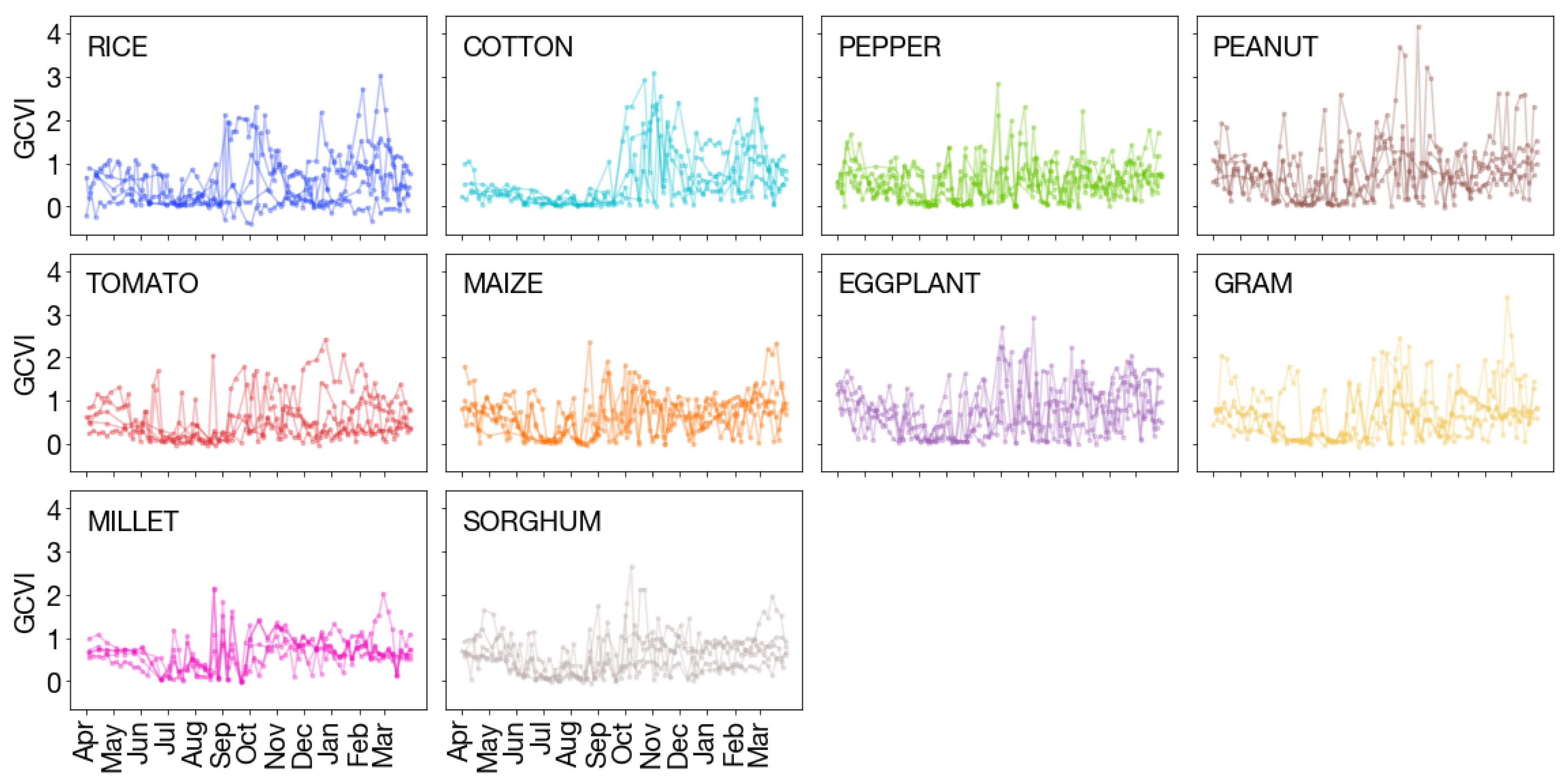
Using Google Earth Engine [45], we exported all Sentinel-2 Level-1C images at each submission coordinate for the corresponding crop year, where a crop year is defined to be from 1 April of one year to 31 March of the next. For example, a Plantix submission from 1 September 2017—during the kharif season—generates a time series of Sentinel-2 readings from 1 April 2017 to 31 March 2018, which encompasses the fall 2017 kharif season and winter 2017–2018 rabi season. 1 April was chosen as the cutoff date to avoid truncating early kharif or late rabi satellite data that could be relevant for crop type classification. All spectral bands were sampled at 10 m ground resolution; the 20 m and 60 m bands were resampled using the GEE default nearest neighbor algorithm. In addition to the 13 spectral bands, we also computed the green chlorophyll vegetation index ( GCVI = NIR / green 1 ) [46] as previous work has shown GCVI to correlate well with leaf area index [47] and be a strong feature for crop type classification [18,48]. Figure 2 visualizes GCVI time series of the 10 crop types and shows the high levels of noise due to clouds in Sentinel-2 imagery.
Across the dataset of Plantix submissions, the median number of Sentinel-2 images for the 2017–2018 crop year was 42, with minimum and maximum image counts of 36 and 143. In 2018, the median image count was 71, with minimum and maximum of 67 and 143. Of these images, many are affected by clouds and cloud shadows, especially during the monsoon season; since the Sentinel-2 Level 1-C cloud mask has a high omission error at the time of writing [49], we describe methods to minimize the impact of clouds in Section 4.3.2. Although we will show that it is possible to make progress in distinguishing crop types in the presence of cloudy imagery, the lack of high-quality cloud mask remains a major challenge to mapping crop types in smallholder systems, and we expect the improvement of such masks to enable better classification performance in the future.

3.3. Sentinel-1 Time Series

The Sentinel-1 constellation is composed of two satellites, Sentinel-1A and Sentinel-1B, launched April 2014 and April 2016, respectively. The satellites carry a C-band synthetic-aperture radar (SAR) instrument that captures 5–40 m resolution imagery with a revisit period of 12 days. We used the Interferometric Wide swatch mode, which acquires images with dual polarization (vertical transmit, vertical receive (VV) and vertical transmit, horizontal receive (VH)). In addition to using backscatter coefficients as features, we computed their ratio and difference ( RATIO = VH / VV = VH dB VH dB and DIFF = VV VH ) based on previous work that indicated the suitability of such transformations for agricultural applications [18,50,51]. Unlike optical imagery, radar is not affected by weather conditions and can monitor the Earth’s surface through clouds, making it a useful complement to optical imagery during the wet season. The median number of Sentinel-1 images available was 30 in both 2017 and 2018, with minimum and maximum of 21 and 78.
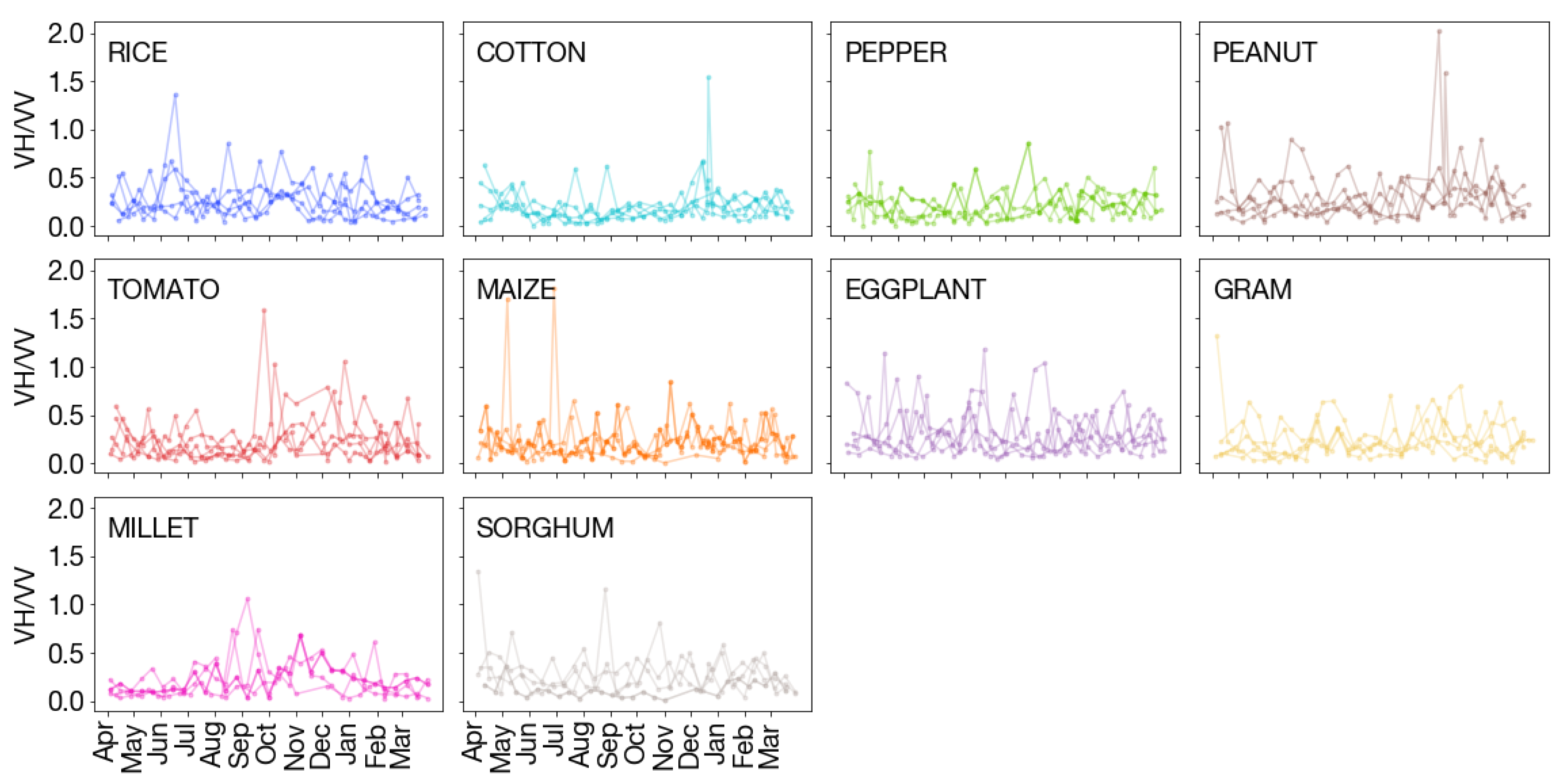
Sentinel-1 Ground Range Detected (GRD) scenes are available in GEE, which processes the imagery using ESA’s Sentinel-1 Toolbox to reduce noise and standardize bands at 10 m spatial resolution. We note that after this processing Sentinel-1 imagery still contains speckle-noise, which is caused by backscatter interference. While speckle is highly disruptive for interpreting individual images taken at one point in time [52], its effect on a SAR time series over the course of a year is dampened by the feature extraction methods described in Section 4.3.2 and Section 4.3.3. We used GEE to export Sentinel-1 GRD observations at each submission coordinate for the corresponding crop year, where a crop year is defined to be from 1 April of one year to 31 March of the next (Figure A2).

3.4. DigitalGlobe Static Satellite Imagery

Due to Android phone location inaccuracy and users taking photos of crops while not standing in their fields (e.g., from the road next to their field or in an urban area with internet access), we employed very high resolution satellite imagery to filter for points within a crop field. A single DigitalGlobe image was downloaded using the company’s Web Map Service application for each submission location, for all 72,000 kharif season submissions (see Section 4.1 for how we arrived at 72,000). Images have 0.3 m ground sample distance, are RGB, and span 256 × 256 pixels (76.8 m × 76.8 m) around the submission location. This ground resolution is high enough for humans to visually determine whether any pixel in the image belongs to a crop field or not.
Since we used time series of Sentinel imagery for crop type classification, we were interested in whether the Sentinel pixel covering each submission location is within a crop field. We therefore drew a 10 m × 10 m square centered within each DigitalGlobe image to approximate the bounds of the corresponding Sentinel-2 pixel.

3.5. Sub-National Crop Area Statistics

District-wise, season-wise crop production statistics were available from 1997 to 2016 on India’s Crop Production Statistics Information System and Open Government Data (OGD) Platform [9,53]. We compared the kharif crop area data in 13 districts of Andhra Pradesh and 30 districts of Telangana against our aggregated crop type predictions. Note that the number of districts in Telangana increased from 10 to 33 upon redistricting in 2016. In the latest government crop statistics (2016–2017), data were only available for 30 of the 33 districts (Hyderabad is urban, Mulugu and Narayanpet missing).

4. Methods

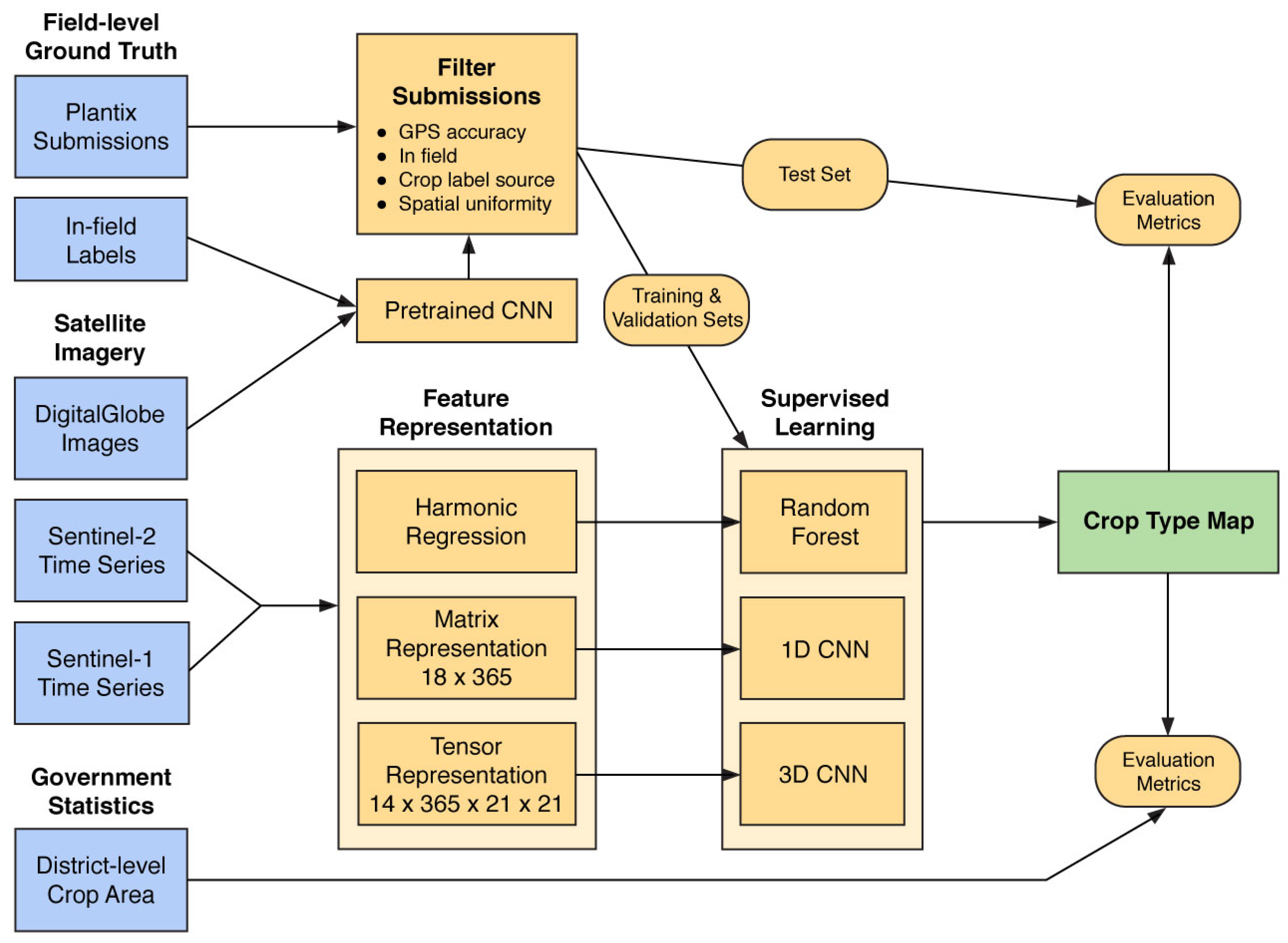
For a graphical overview of the methods presented in this paper, please see Figure 3.

4.1. Measuring and Reducing Noise in Crowdsourced Data

4.1.1. Initial Filtering by PEAT

To extract usable data and minimize noise, our collaborators at PEAT applied several filtering steps to the original 1.8 million submissions. First, photos had to show a crop (1.3 million samples) and be labeled by an expert or with a Plantix-DNN prediction consistent with disease prediction (1.0 million samples). Second, the predicted crop type had to be one of a pre-selected list of crops: rice, cotton, peanut, pepper, tomato, eggplant, maize, gram, millet, and sorghum (620,000 samples), which account for about 70% of the region’s kharif crops (Table 1). Third, Android location accuracy had to be available and within 200 m (213,000 samples). Lastly, only one image of each crop type was permitted per user (102,000 samples). This minimized the overrepresentation of very active users and submissions from the same field.
Since there are two growing seasons in southeast India, we chose to focus on kharif crops to simplify the classification task. We defined kharif samples as those submitted between 1 June and 1 December, which filtered the dataset further to 72,000 samples. A geographic and temporal distribution of Plantix submissions in our study region is shown in Figure 1, and a quantitative summary by crop type, with comparisons to government statistics, can be found in Table 1. Rice is by far the most highly represented crop type in Plantix submissions with over 32,000 points, followed by cotton with over 10,000. All other crop types have below 10,000 submissions. It is worthwhile to note that, between the selection bias of submission through the Plantix app and filtering for usable samples, this dataset is likely to contain biases; we discuss these in more detail in Section 6.
The dataset of 72,000 kharif samples, though filtered, still included many noisy submissions. Below, we describe methods to further filter the dataset on Android location accuracy, how much of the Sentinel-2 pixel is within a crop field, whether crop type was assigned by a human expert or by the Plantix-DNN, and spatial uniformity across the study region.

4.1.2. Android Location Accuracy

Information on the location accuracy of submissions was available via the Android platform. The Android Location API supplied the horizontal accuracy of a location as the radius of 68% confidence. In general, higher accuracy in location required higher battery drain, so preservation of battery life compromised location accuracy and therefore the majority of submissions’ usefulness for crop type mapping. Filtering for submissions with accurate locations is a crucial step in de-noising crowdsourced data.
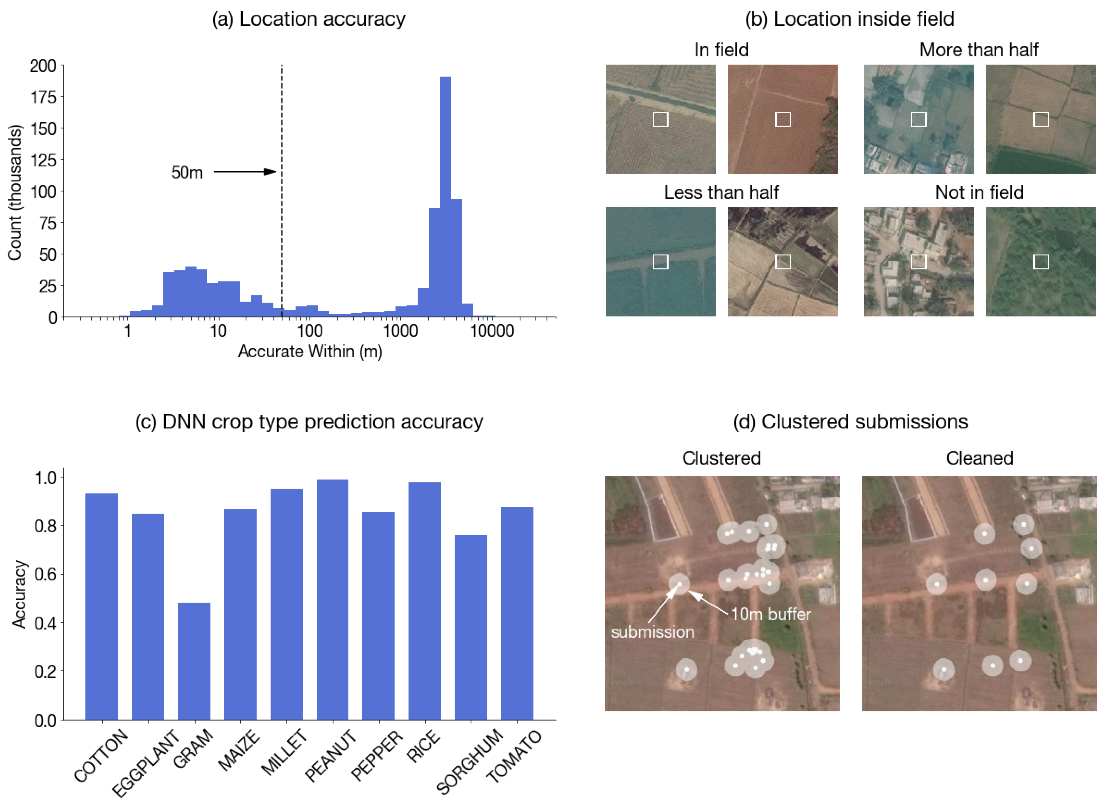
A histogram of submission location accuracy across a random sample of the 1.8 million dataset is shown in Figure 4a. The distribution is bimodal, with one small peak at 5 m and a second, much larger one at 3000 m. In comparison, the average operational holding size in AP and Telangana is 0.94 ha and 1.00 ha, respectively [28], and we observed individual fields as small as 10 × 10 m in DigitalGlobe imagery. This implies that a location accurate to 200 m is unlikely to still be inside the field of the submitted photo. We filtered for location accuracies at the 10 m, 20 m, and 50 m level in our sensitivity analyses; submissions with accuracies >50 m were discarded. Note that, since the Android location service seeks to preserve battery at the expense of accuracy, the ≤50 m criterion alone removes 61% of all submissions.

4.1.3. Pretrained CNN for In-Field Classification

A second source of label error is the farmer taking a photo of a plant without standing inside their field. They often take the photo from a road at the edge of their field, pick off a diseased leaf, and photograph it in an urban area (i.e., in a place with WiFi), or stand under trees in fields while using the app. Though the crop type labels may be correct for the submitted photos, the satellite time series at these non-field locations do not correspond to those labels.
We used the DigitalGlobe (DG) imagery described in Section 3.4 and a 2D CNN to classify each submission into one of four classes: “in field”, “more than half”, “less than half”, and “not in field” (Figure 4b). The rationale for finer-grained labels “more than half” and “less than half” is that the spectral reading at a pixel that is mostly in a field may be dominated by the crop in that field, whereas pixels mostly not in one field are too mixed or contaminated.
Since the DG images are RGB, we classified them using well-established network architectures designed for natural images. We tried two commonly-used CNN architectures: VGG and ResNet [54,55], each with two network depths (VGG-11, VGG-19, ResNet-18, and ResNet-50). Their weights were initialized by pretraining on the large RGB image database ImageNet to boost classification accuracy with small training sets [56]. All four pretrained initializations were available off-the-shelf in the deep learning framework PyTorch [57]. We also tried two resolutions of DG imagery: 0.3 m and 0.6 m, the latter of which was downsampled from the 0.3 m imagery. At both resolutions, images were cropped to 224 × 224 -pixels to fit the pretrained models.
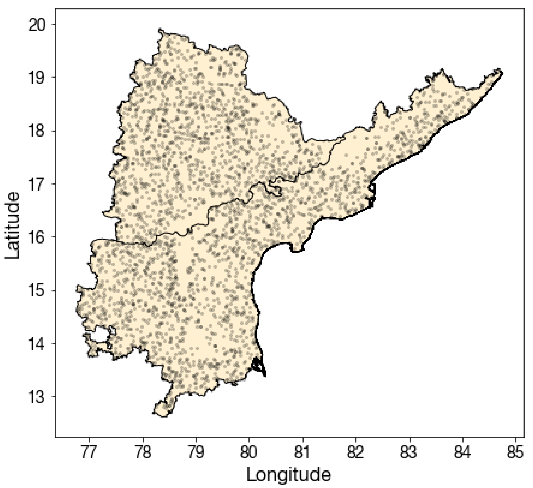
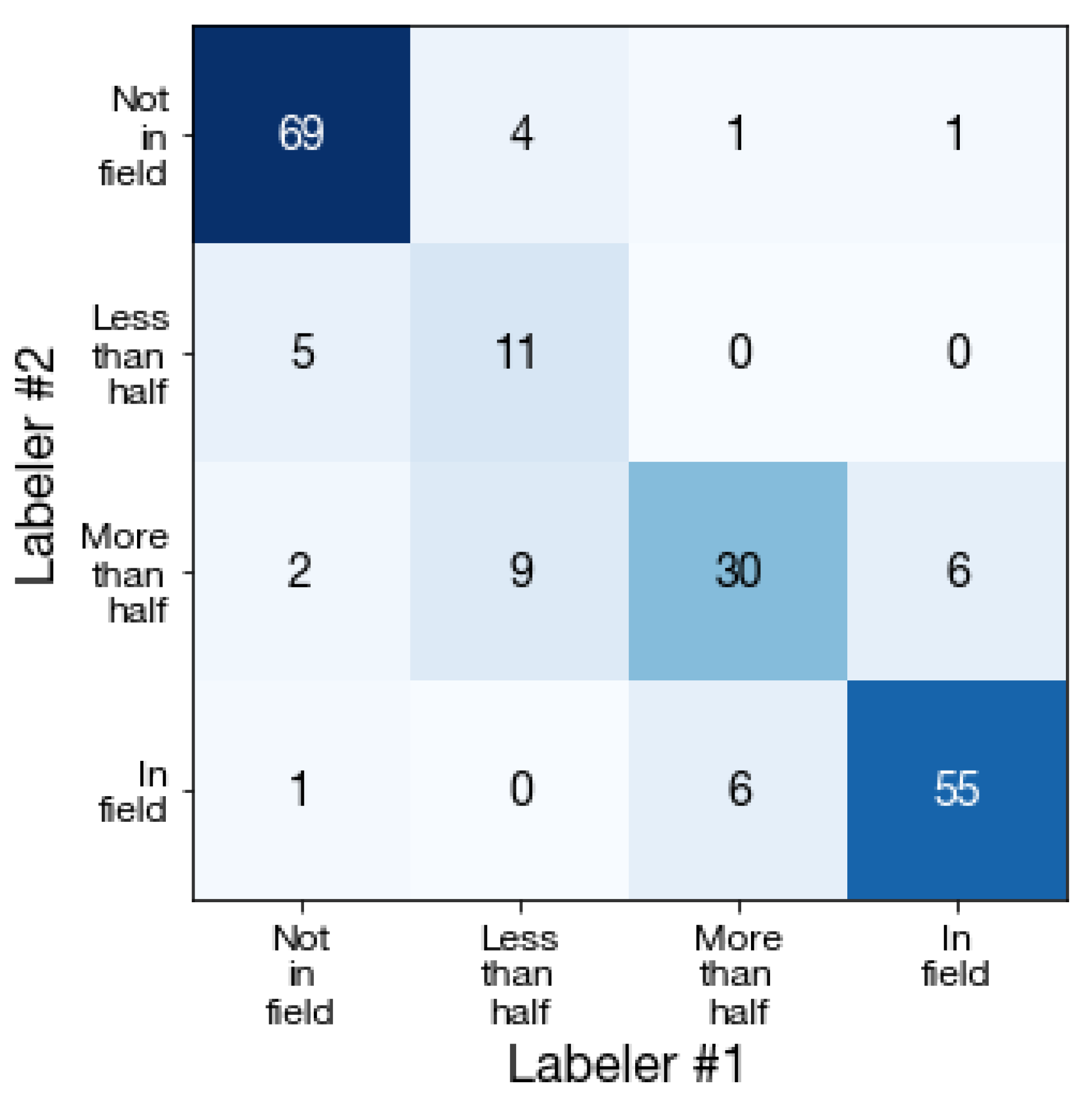
We sampled 3000 submissions from the 72,000 kharif points obtained at the end of Section 4.1.1 in a geographically uniform manner (Figure A3). Through manual inspection of the DG images, which took a total of 4 hours, two human labelers generated in-field labels to train the CNNs. Figure A4 shows the agreement between the two labelers to give a sense of the task difficulty. Of these 3000 DG images, 2000 were placed in the training set, 500 in the validation set, and 500 in the test set; each split was constructed so that no points in one split were within 200 m of any points in the other two splits (to ensure non-overlapping DG images). Table 2a summarizes the distribution of labels.
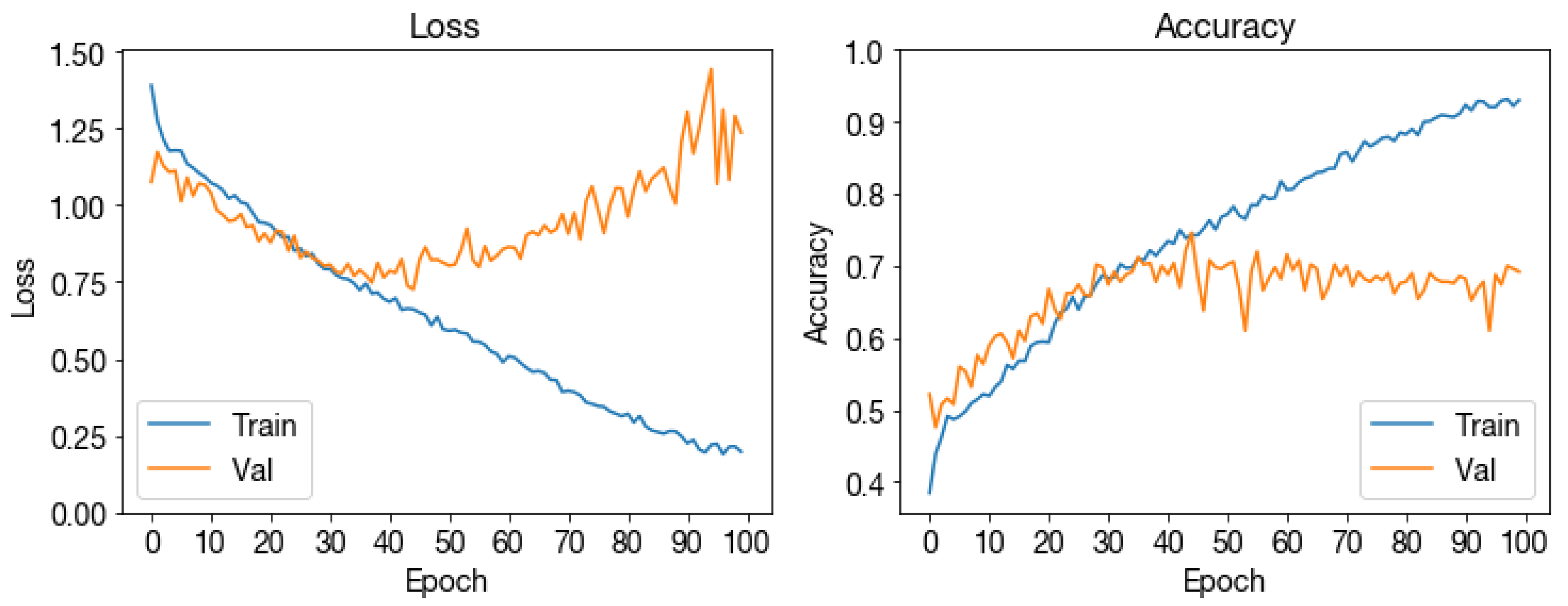
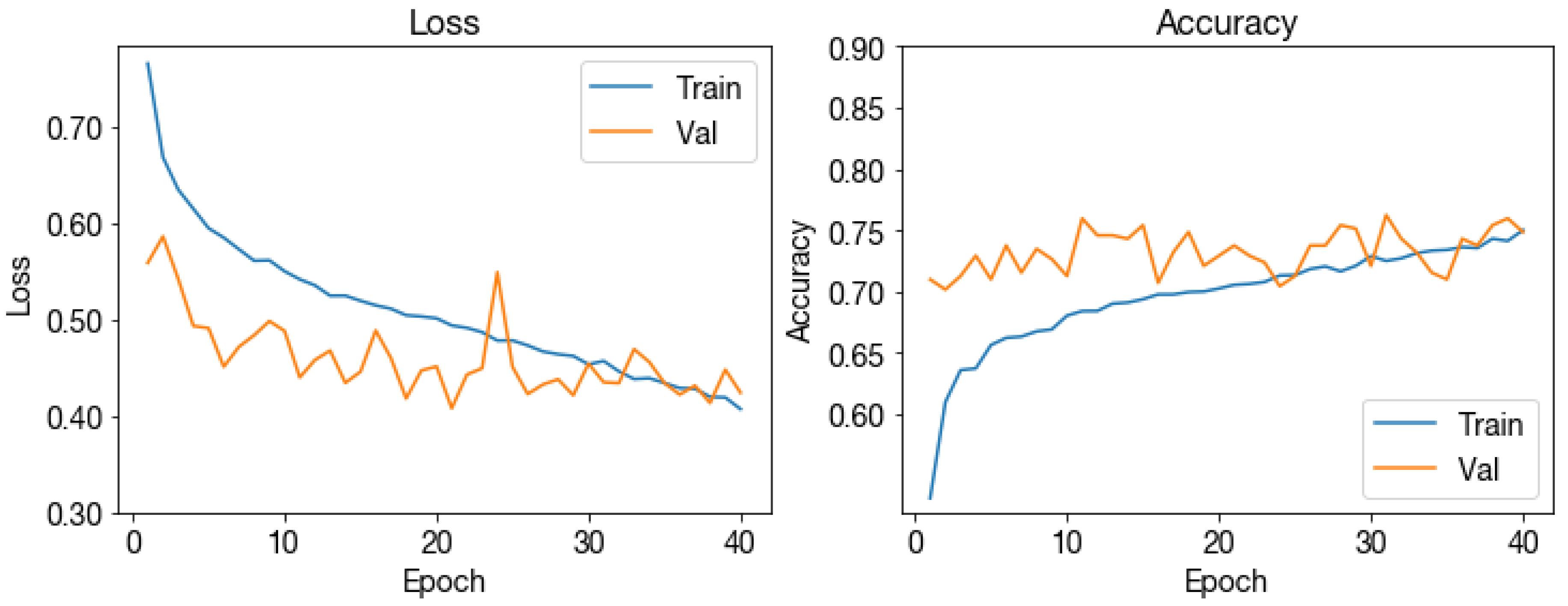
The CNNs were trained to minimize cross entropy loss (Equation (2)) with C = 4 for the four classes. During training, common data augmentation strategies were used to increase the diversity of the training set: random horizontal flips, vertical flips, rotations, and color jitters. The best model was selected via the highest validation set accuracy, and test set accuracy was evaluated using this model. Details of the network architectures and optimization parameters are shown in Table A1, training loss and accuracy over epochs are shown in Figure A5, and pretrained networks’ validation set accuracies are shown in Table A2.
We note that this data cleaning step significantly reduces noise found in the Plantix dataset, but remains imperfect. CNN misclassifications aside, it is unclear which field a submission is from when it is on the boundary between two fields, but the submission may still be considered “more than half” in a field. Geolocation errors of Sentinel-2 images (especially Sentinel-2B prior to mid-2018), which we did not correct, may also add noise to the time series of submissions near field boundaries [58]. We therefore tested different in-field thresholds for inclusion in the training set and report their effect on performance in the results.

4.1.4. Expert vs. Plantix-DNN Labeling

Since the vast majority of crop type labels were assigned by Plantix’s deep neural network (DNN) trained on expert labels, the use of these imperfect labels introduces another source of noise. Figure 4c shows the DNN accuracy by crop type, evaluated on the expert labels. The overall accuracy is 97%, while crop-specific recalls range from 48% for gram to 99% for peanut. Accuracies for rice and cotton are 97% and 93%, respectively. In the sensitivity analyses, we compared the performance of models trained on expert-labeled submissions to those trained on DNN-labeled submissions.

4.1.5. Spatial Distribution of Submissions

The geographic distribution of submissions is heavily concentrated around urban areas (e.g., Hyberadad) and locations of highly-active users (Figure 1), likely due to differences in smartphone ownership, internet access, and knowledge of the Plantix app. One field may generate multiple submissions when its farmer is an active user. We introduced another filtering step in which submissions within 20 m of another were considered duplicates and removed (Figure 4d).

4.2. Constructing Training, Validation, and Test Sets

Identifying a good crop type classifier and providing an unbiased out-of-sample estimate of classification performance requires validation and test sets that (1) have high label accuracy and (2) are representative samples of the region. To generate cleaned validation and test sets, we first filtered for the set of points that satisfied the following criteria.
1.
The location accuracy is deemed to be ≤10 m by the Android platform.
2.
The Sentinel-2 pixel at the submission location has been classified as either “in field” or “more than half” inside a field.
3.
A crop scientist, not the DNN, assigned the crop type label based on the submission photo.
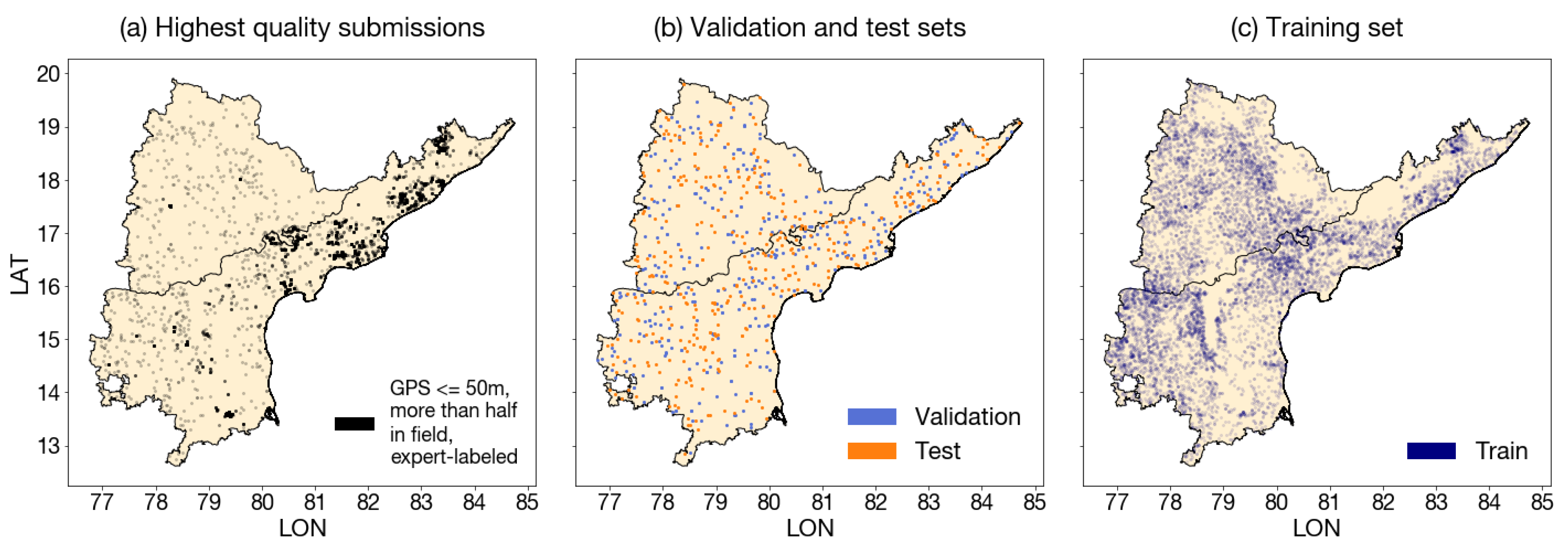
The resulting dataset was heavily skewed toward the eastern part of the study region (Figure A8a), undermining the ability of the validation set to select a good model for the entire region and of the test set metrics to represent the entire region. To achieve greater spatial uniformity, we started with an empty set, randomly sampled coordinates within the study region, and added the “clean” submission closest to the sampled coordinate until the validation and test sets each reached 400 samples (Figure A8b).
In these cleaned validation and test sets, the median location accuracy was 4.6 m and 4.1 m, respectively. This means that the sample has on average a 68% chance of being within 4.6 m (or 4.1 m) and a 95% chance of being within 9.2 m (or 8.2 m) of the submission location. Forty-one percent of the validation set were classified as completely inside a field, while 43% of the test set were completely in-field.
To see how much validation set noise affects the ability to choose good training data and models, we also constructed a noisy validation set comprised of 400 points sampled at random from the original dataset. It therefore includes submissions with GPS accuracy from 10–50 m, submissions not taken inside a crop field, and submissions labeled by the Plantix-DNN. Note that, to avoid overfitting and inflated metrics, no samples in the validation or test sets were within 500 m of samples in the other two sets.
The training set was derived from the remaining points in the dataset not in the validation and test sets (Figure A8c). Training points were filtered to be at least 500 m from all points in the validation and test sets (45,000 samples), to have Sentinel-2 pixels in field or more than half in a field (21,000 samples), and to not contain points within 20 m of each other. The final training set used to train the classifiers contained 9079 samples, a very large reduction from the 1.8 million raw submissions.

4.3. Crop Type Classification

As a result that smallholder systems are highly heterogeneous and simple rules to separate crop types are not immediately apparent (Figure 2), we tested the performance of three machine learning algorithms for feature extraction and crop type classification (Figure 5). The first is a random forest using features derived from harmonic regressions on satellite time series, an algorithm that has performed well at crop type classification in previous studies [18,36]. The second is a 1D CNN with kernels convolving over the temporal dimension of the time series. The advantage of a CNN is that features are learned, not prescribed, and can take useful forms that the harmonic coefficients cannot. The third model is a 3D CNN with kernels convolving over two spatial and one temporal dimension of the time series for an entire image tile. The 3D CNN can see a broad spatial context that the previous two methods cannot, but it contains more parameters, is much more computationally intensive to train, and is more prone to overfitting on small datasets. A comparison of the data storage and computational runtime required for each model is provided in Table A3.

4.3.1. Choosing Crop Types to Predict

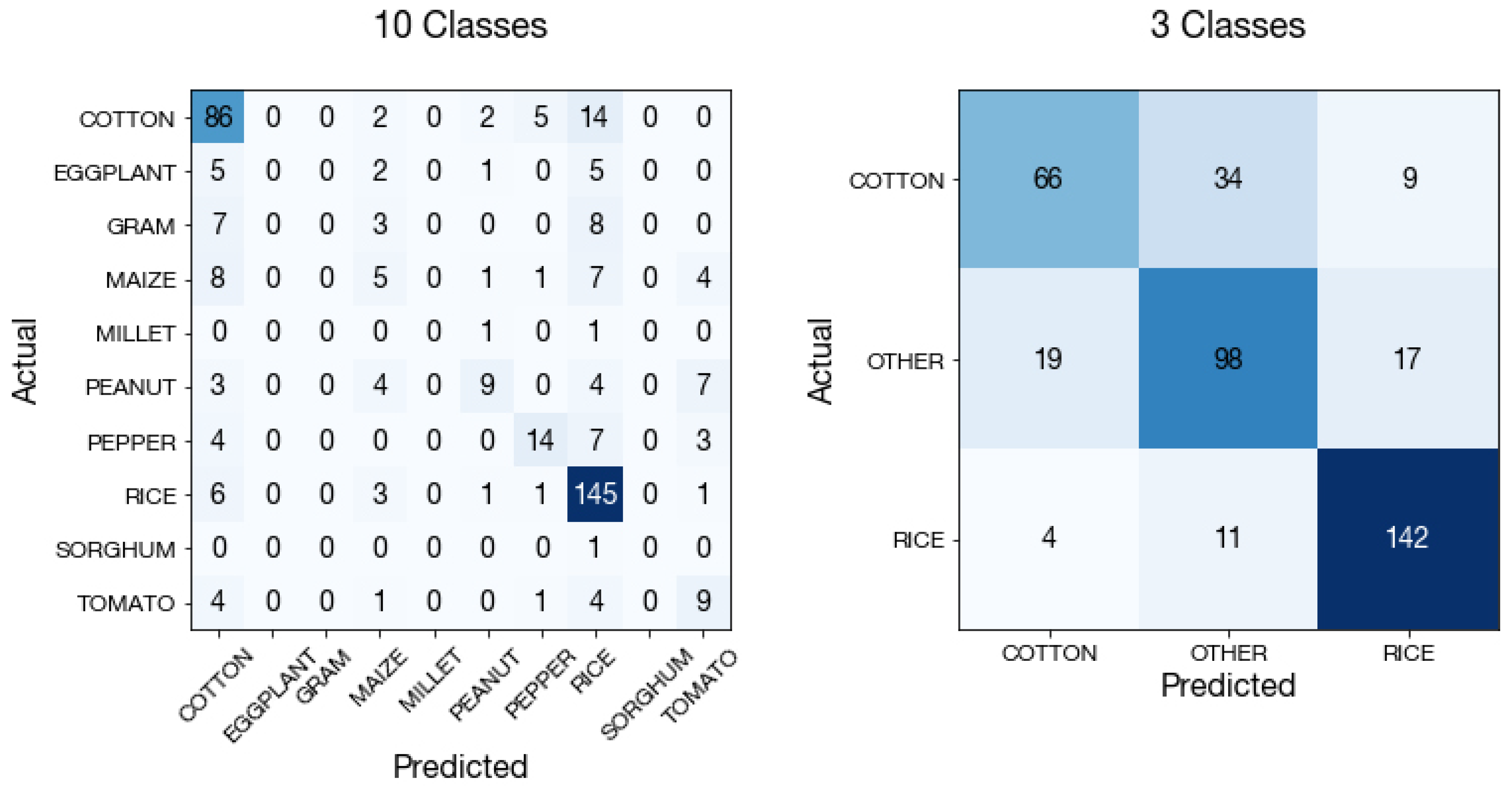
The Plantix dataset contains ten crop types, whose distribution is shown in Table 1. Ideally, a classifier would achieve high precision and recall on all ten crops; in reality, the minor crop types do not have enough label quantity or signal in their time series for accurate classification. We first show results for 10-crop classification to demonstrate the difficulty of mapping minor crops over large geographic extents with only small label quantities. We then simplify the classification to a 3-class problem of distinguishing rice and cotton from all other crops (lumped into one “other” class). Rice and cotton were chosen because they are the two major kharif crops in Andhra Pradesh and Telangana (Table 1), had label accuracy exceeding 90% from the Plantix DNN (Figure 4c), and had high precision and recall in the 10-crop classification task (Figure A13).

4.3.2. Random Forest with Harmonic Features

In order to use the phase and amplitude of plant phenology to differentiate crop types, a method is needed to transform variable-length discrete time series into features that can be input into machine learning algorithms. One such method whose features have been successfully used to classify crop types is the harmonic regression, or regression using a Fourier basis [18,34,35,36]. The harmonic regression decomposes a function of time into its frequencies, yielding a compact representation of the time series at each satellite band or vegetation index (VI). Mathematically, it is equivalent to performing a discrete Fourier transform [59].
We viewed each satellite band or VI as a time-dependent function f ( t ) and performed the harmonic regression
f ( t ) = c + k = 1 n a k cos ( 2 π k t ) + b k sin ( 2 π k t )
for each band/VI independently, where a k are cosine coefficients, b k are sine coefficients, c is the intercept term, and n is the order of the harmonic series. The independent variable t represents the time an image is taken within a crop year expressed as a fraction between 0 (1 April) and 1 (next 31 March).
Due to the presence of clouds, the harmonic regression fit naively to a Sentinel-2 time series does not capture crop phenology well. In the absence of an accurate cloud mask, we followed a recursive curve fitting procedure similar to that implemented in the TIMESAT program [60], which has been shown to reduce the bias introduced by clouds. The algorithm recursively fits the harmonic regression to the time series, and then imputes the cloud-free values of the time series by taking the maximum (or minimum) of the band/VI and the regression fit if clouds appear as low (or high) values for that band/VI. For example, since clouds appear as low GCVI values, one iteration of the recursive algorithm would regress the raw GCVI values on the harmonic terms, then take the maximum of the fitted curve and the raw GCVI values. This can be repeated for a total of r recursive fits (Figure 5a).
The values of n and r are hyperparameters that must be tuned via cross-validation for a given dataset and task. A larger n (more cosine and sine terms) increases model flexibility but risks the model overfitting to spurious patterns. Meanwhile, r should minimize the influence of clouds on the coefficients without obscuring real phenological signal. We picked n = 3 and r = 2 by minimizing crop type classification error on a hold-out set (Table A4).
After performing this regression recursively, we extracted coefficients a 1 , a 2 , a 3 , b 1 , b 2 , b 3 , and c for each of the 18 bands and VIs, giving us a total of 126 features on which to classify crop types. Since the model has seven parameters to fit, it requires at least seven cloud-free observations at a pixel to extract meaningful coefficients, a criteria that is met at all Sentinel-1 and Sentinel-2 pixels (Section 3.2). An example regression is shown in Figure 5a for GCVI on a rice submission time series.
Finally, to perform crop type classification, we trained random forest models with the harmonic coefficients as input and Plantix-labeled crop type as output. Random forest is an ensemble machine learning method comprised of many decision trees in aggregate [37], and has frequently been used in the field of remote sensing to perform land cover classification and crop type mapping [61,62]. It often yields higher accuracy than maximum likelihood classifiers, support vector machines, and other methods for crop type mapping [14,34,63,64]. We used the default parameters of Python’s scikit-learn [65] package RandomForestClassifier with the exception of increasing n_estimators (the number of decision trees in the random forest) from 10 to 500 to reduce model variance. Error bars on classification metrics were obtained by fitting the classifier on multiple bootstrapped training sets (sampled with replacement).

4.3.3. 1D Convolutional Neural Network

While random forests are commonly used for crop type mapping in the literature [14,18,36], obtaining features for the model still require the user to assume a functional form to summarize time series data. In contrast, neural networks learn both the feature representations from the raw data as well as how to use them to perform classification. If harmonic coefficients fail to capture some information that is helpful for classifying crop types, or random forests are not well-suited to learn the types of nonlinearities that characterize decision boundaries, a neural network has the potential to perform better.
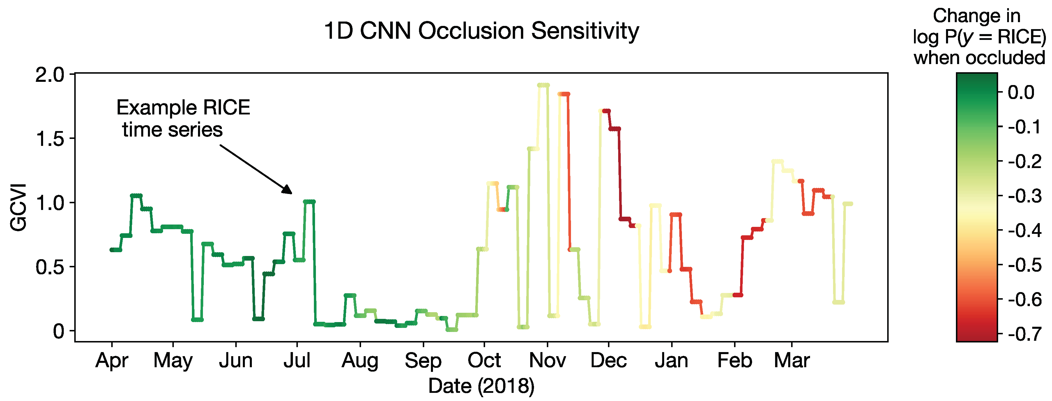
To classify satellite time series, we constructed a 1D convolutional neural network. The time series for each sample was represented as an 18 row × 365 column matrix, where each row is a band/VI and each column is a day of the year. The first 14 rows are Sentinel-2 bands and GCVI, and the last 4 rows are Sentinel-1 VV, VH, RATIO, and DIFF. This encoding was chosen to standardize Sentinel-1 and Sentinel-2 time series with different observation dates to the same neural network input size. If a satellite took an observation on day D, then column D in the matrix will be filled with that satellite’s band values (Figure 5b). Since the revisit times of Sentinel-1 and Sentinel-2 are 6 and 5 days, respectively, the values on days with no observation were imputed with values from the previous observation (known as “forward imputation” [66]). Lacking a high quality cloud mask for Sentinel-2, we again were not able to remove cloudy observations. As a result that neural networks can learn which parts of an input are relevant to the task at hand [67,68,69] and have previously been shown capable of ignoring cloudy observations [70], we did not further process the time series to reduce the influence of clouds, as we did for the random forest classifier. An occlusion sensitivity analysis, shown in Figure A15, shows that the 1D CNN indeed learns to rely largely on clear observations for classification.
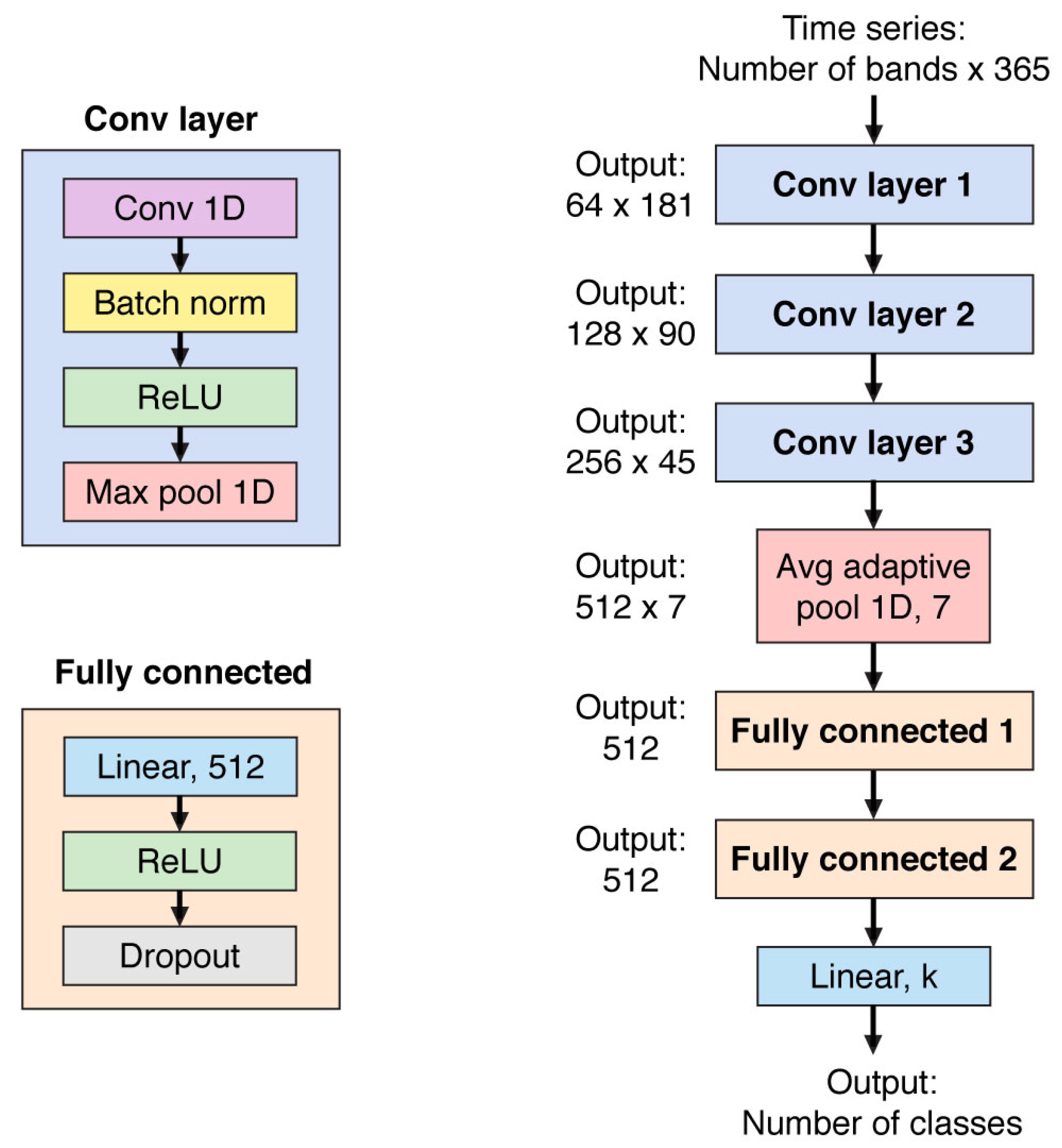
In image classification, convolutions are 2D and are performed across the two spatial dimensions of the image. Here, each submission is comprised of one pixel and there are no spatial dimensions; the CNN instead convolves over the temporal dimension with kernels of size 3. The 1D CNN architecture is comprised of multiple convolutional blocks, each of which is a stack of 1D convolution, batch normalization, rectified linear unit (ReLU), and 1D max pooling layers (Figure A11). The final prediction is output by a few fully connected layers.
Training was performed by minimizing the cross entropy loss, defined as a function of the ith input sample as
( θ , x , y ) = c = 1 C y c log y ^ c
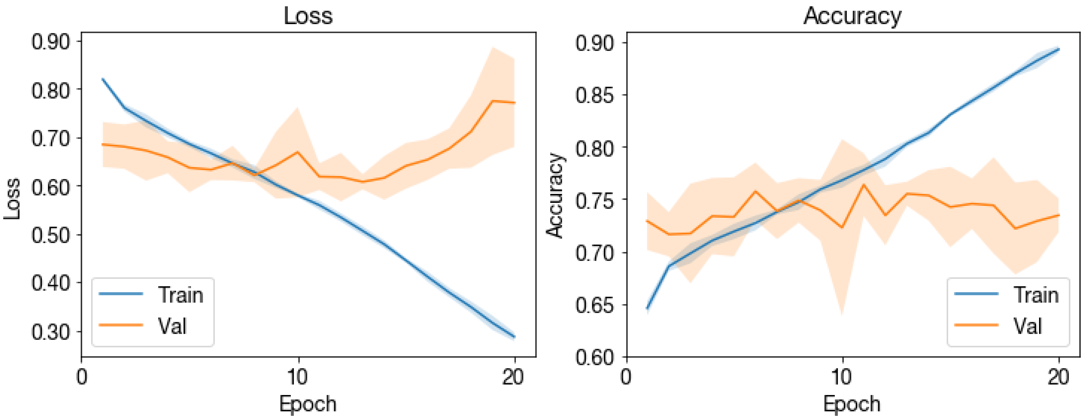
for model parameters θ , number of classes C, the input time series x , crop type probabilities y ^ = f θ ( x ) , and one-hot ground truth label y . The notation y c denotes the cth element of the vector y , which is equal to 1 if the sample belongs to class c and 0 otherwise. The element y ^ c is the predicted probability that the sample belongs to class c. Minimizing cross entropy incentivizes the network to maximize the value of y ^ c for the correct class c. Figure A12 shows a typical training curve for the 1D CNN.
Hyperparameters, such as the number of convolutional blocks and the number of filters per layer, were chosen to maximize prediction performance on a validation set and are shown in Table A6. The model that performed the best on the validation set was a CNN with 4 layers, 64 filters in the first layer, a learning rate of 0.001, and a batch size of 16. Other implementation details can be found in Table A5.

4.3.4. 3D Convolutional Neural Network

A limit of the 1D CNN is that it is only able to use temporal information to classify crop types; it does not “see” the spatial context that includes clues like field size and shape, surrounding vegetation, and proximity to buildings and roads. To see whether spatial information can improve crop type classification, we built a 3D U-Net, modeled after the popular 2D U-Net for image segmentation [71].
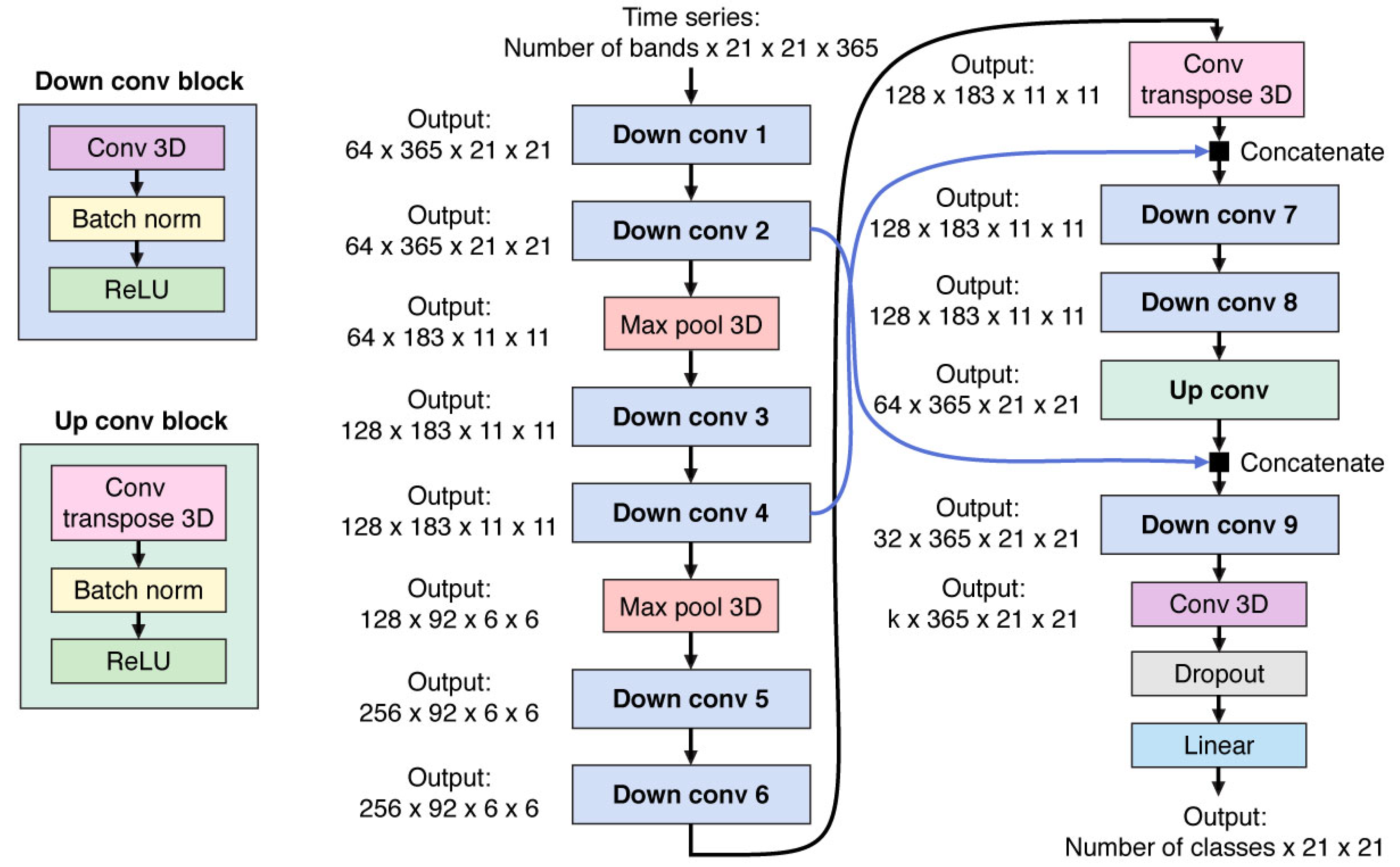
A 21 × 21 pixel tile of each Sentinel-2 image was exported around each submission coordinate to allow spatial features to inform crop type classification. We did not export Sentinel-1 tiles, as the additional storage and computational runtime (Table A3) was high compared to the marginal benefit SAR brought to CNNs in this setting (Table A7). The input to the 3D U-Net is therefore a 4D tensor of size 14 × 365 × 21 × 21 , where days with no Sentinel-2 observation are imputed with the previous observation. Thus the network sees not only the labeled pixel’s time series, but also the time series of pixels up to 200 m away (Figure 5c). The tensor is first downsampled (encoded) via blocks of 3D convolution, batch normalization, ReLU, and 3D max pooling operations in the first half of the network, then upsampled (decoded) back to its original resolution in the second half. A diagram of the network is shown in Figure A16.
The output of the network is a 21 × 21 -pixel segmented prediction in which every pixel is assigned a crop type label. Since we only observed the label at one pixel in the image (Figure 5c), we only computed the loss and performance metrics at that pixel. Like the 1D CNN, the 3D U-Net was trained using a cross entropy loss with C classes (Equation (2)). Figure A17 shows a typical training curve for the 3D CNN.

4.4. Feature Importance via Permutation

We performed experiments to determine the relative importance of features to crop classification by permuting each feature across all samples, as suggested in [37]. The algorithm is as follows.
1.
Fit a classifier to the training set (e.g., harmonic coefficients and random forest, 1D CNN).
2.
Record the baseline predictive performance of the model on the validation set (i.e., accuracy).
3.
For each feature j, randomly permute feature j in the validation set, thereby breaking the association between feature j and the label y. Apply the model to this modified validation set, and record the model performance.
4.
The feature importance is the difference between the baseline performance and the permuted performance.
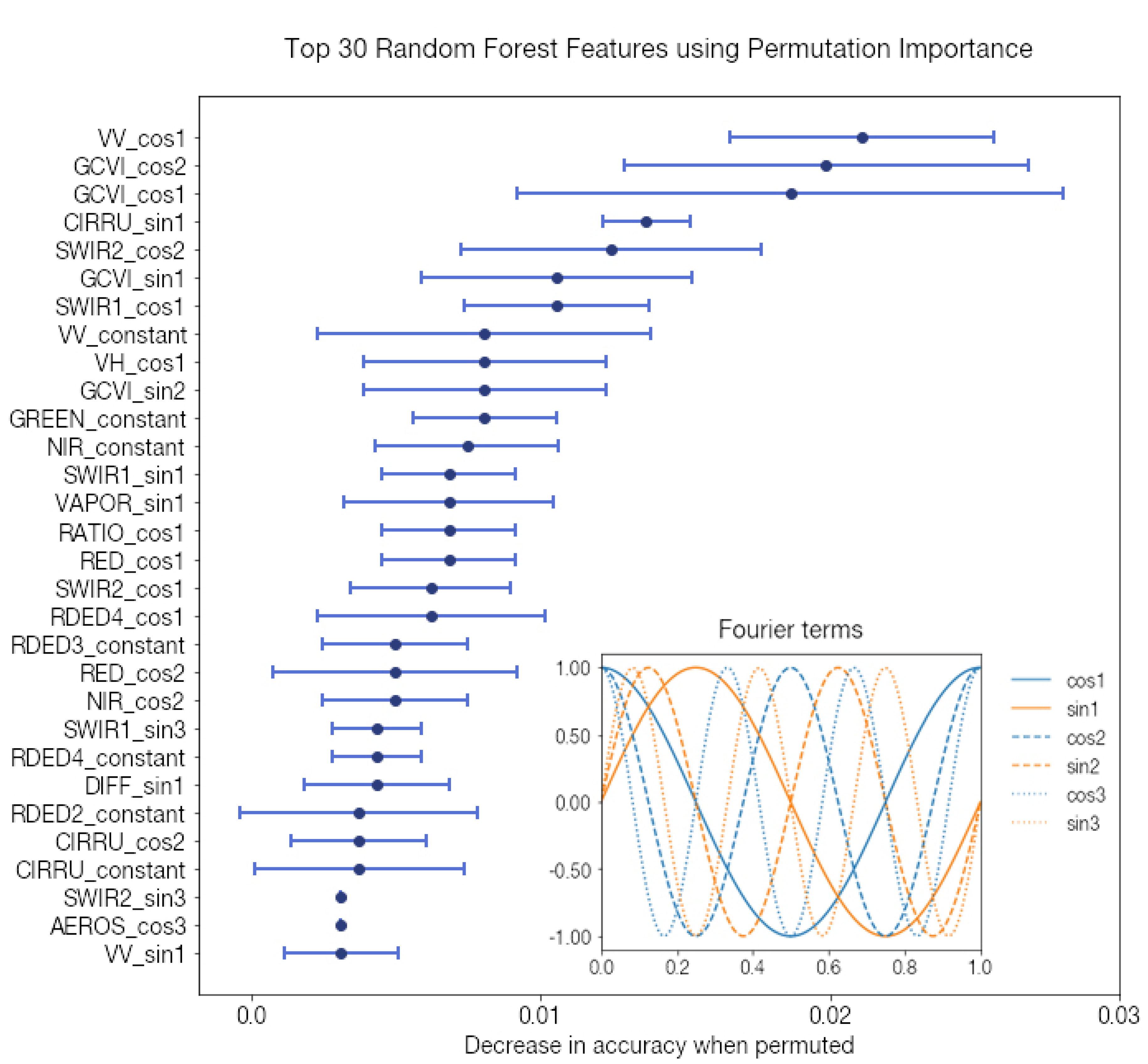
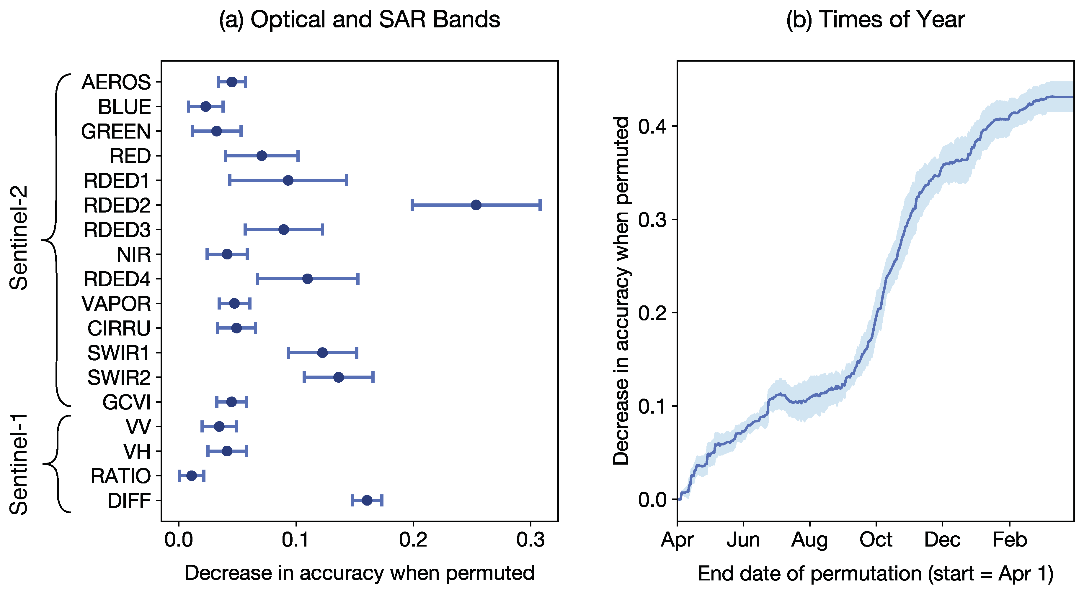
We applied this algorithm to the 126 harmonic coefficient features with the random forest classifier to see which bands and Fourier frequencies decrease classification accuracy the most when permuted. With the 1D CNN, the spectral and temporal dimensions were permuted independently to study which bands and times of year are most important to distinguishing crops. Band b was permuted across all time steps with the same band from another sample, or, for each time step t, all bands were permuted with those of another sample from 1 April to date t.
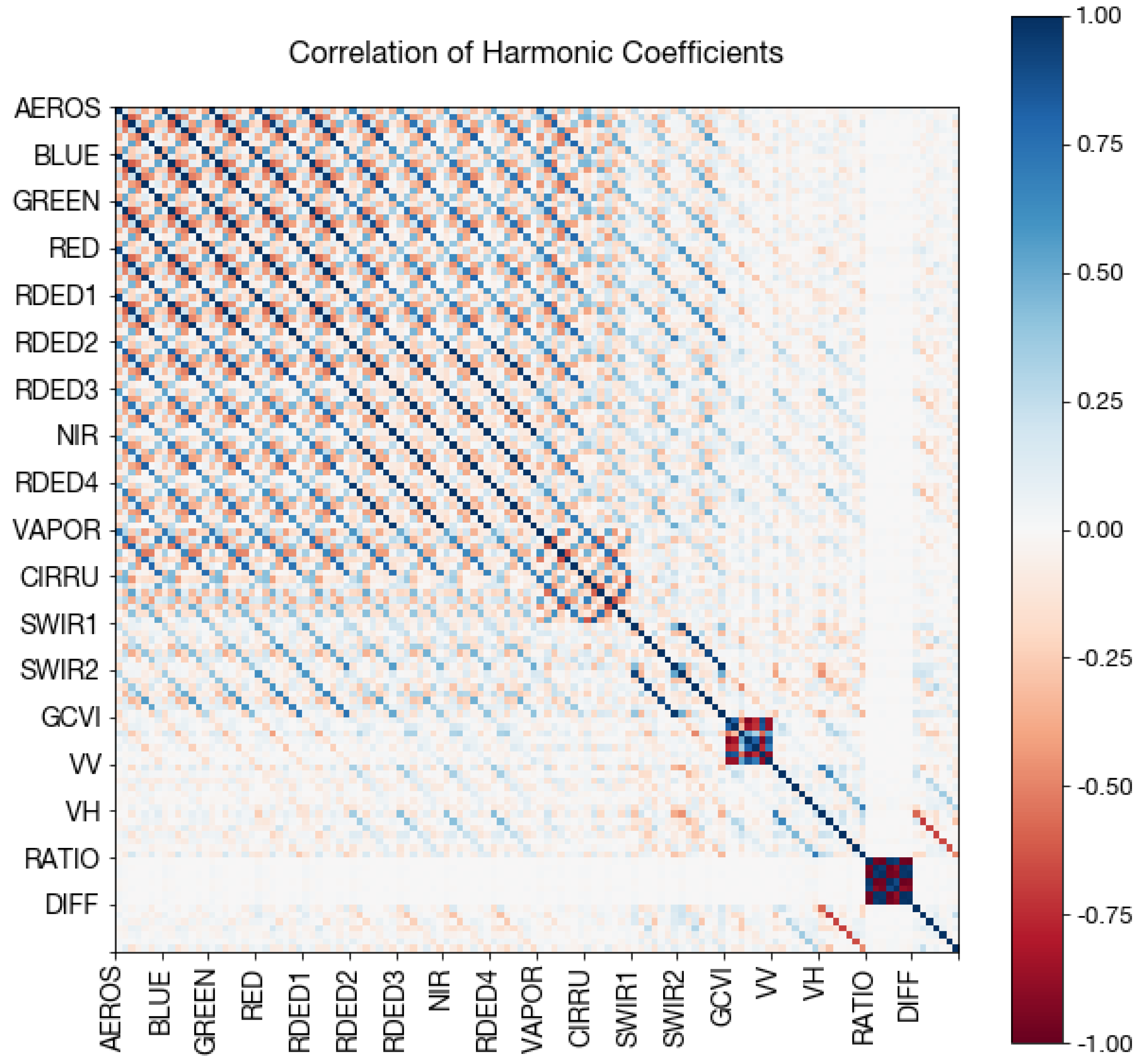
Note that a feature’s importance via permutation is not the same as how much worse a model would perform if trained without that feature, due to correlations between features. That is, a model trained without a particular feature can rely more on other correlated features to compensate. For a correlation matrix of the harmonic coefficients, see Figure A9.

4.5. Assessing the Additional Value of Sentinel-1

As a result that the use of Sentinel-1 for crop type mapping is relatively recent and its utility is not fully known, we performed experiments in which we classified crop types using only Sentinel-2 time series and compared performance to using both Sentinel-2 and Sentinel-1. We compared results for both the harmonics/random forest model and the 1D CNN.

4.6. Validation Against District-Wise Production Data

We sampled ten thousand points uniformly at random from the study region in areas classified as cropland by the Global Food Security-support Analysis Data (GFSAD) Cropland Extent 30 m map [72] and exported all images taken at these points by Sentinel-2 and Sentinel-1 in the period 1 April 2018–31 March 2019. We then used the highest-performing 1D CNN trained on Plantix labels to classify the unlabeled samples into 3 classes (rice, cotton, and other), where rice and cotton had the highest precision and recall among all 10 crops. We compared the percent of samples classified as each crop to the percent of cropland devoted to each crop in 2016–2017 district-level statistics. At the time of writing, statistics were not yet available for 2017–2019, so they predate our classified samples by two years. We exported samples for the 2018–2019 kharif season instead of 2017–2018 because the former has more frequent Sentinel imagery.

4.7. Study Region-Wide Crop Type Map

Using Google Earth Engine, we computed harmonic features on Sentinel-1 and Sentinel-2 bands (Section 4.3.2) across Andhra Pradesh and Telangana for the crop year 1 April 2018 to 1 April 2019. Ten thousand Plantix points from the 2017–2019 kharif seasons were sampled as described in Section 4.2 and used as training points in an Earth Engine random forest classifier with 500 trees. The points were labeled with one of three kharif crop classes: rice, cotton, and other crops. The trained random forest was then applied to all Sentinel pixels in the rest of the region to predict among the three crop classes. We used the harmonic features and random forest for map creation due to their ease of scalability in Earth Engine, as the entire study region contains over 2.7 billion Sentinel pixels. Lastly, we masked out pixels that were not deemed to be cropland by the GFSAD cropland product [72].

5. Results

5.1. DigitalGlobe Images for In-Field Classification

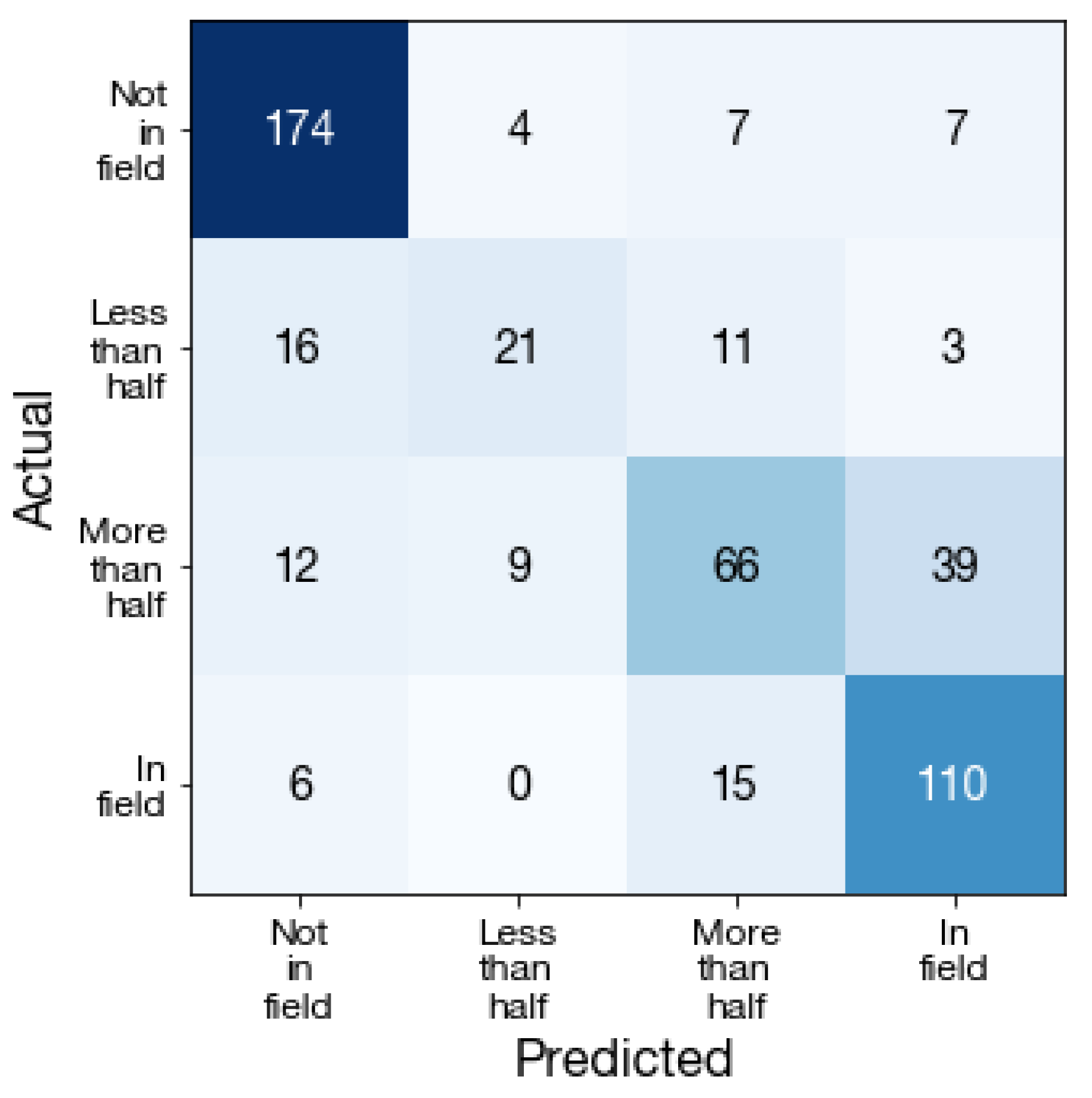
Pretrained convolutional neural networks fit to our in-field dataset ( n = 2000 ) were able to classify whether the center boxes are in-field with high accuracy. The best model, a pretrained ResNet with 18 layers using 0.3 m resolution DigitalGlobe imagery (Table A2), distinguished between center boxes that are completely, more than half, less than half, and not in a field with 74.2% test set accuracy (Table 2b). Comparison to the baseline accuracy (guessing majority class) of 38.4% and human labeler agreement of 82.5% (Figure A4) indicates that the ResNet performed considerably better than the baseline on a task that can often be confusing to humans.
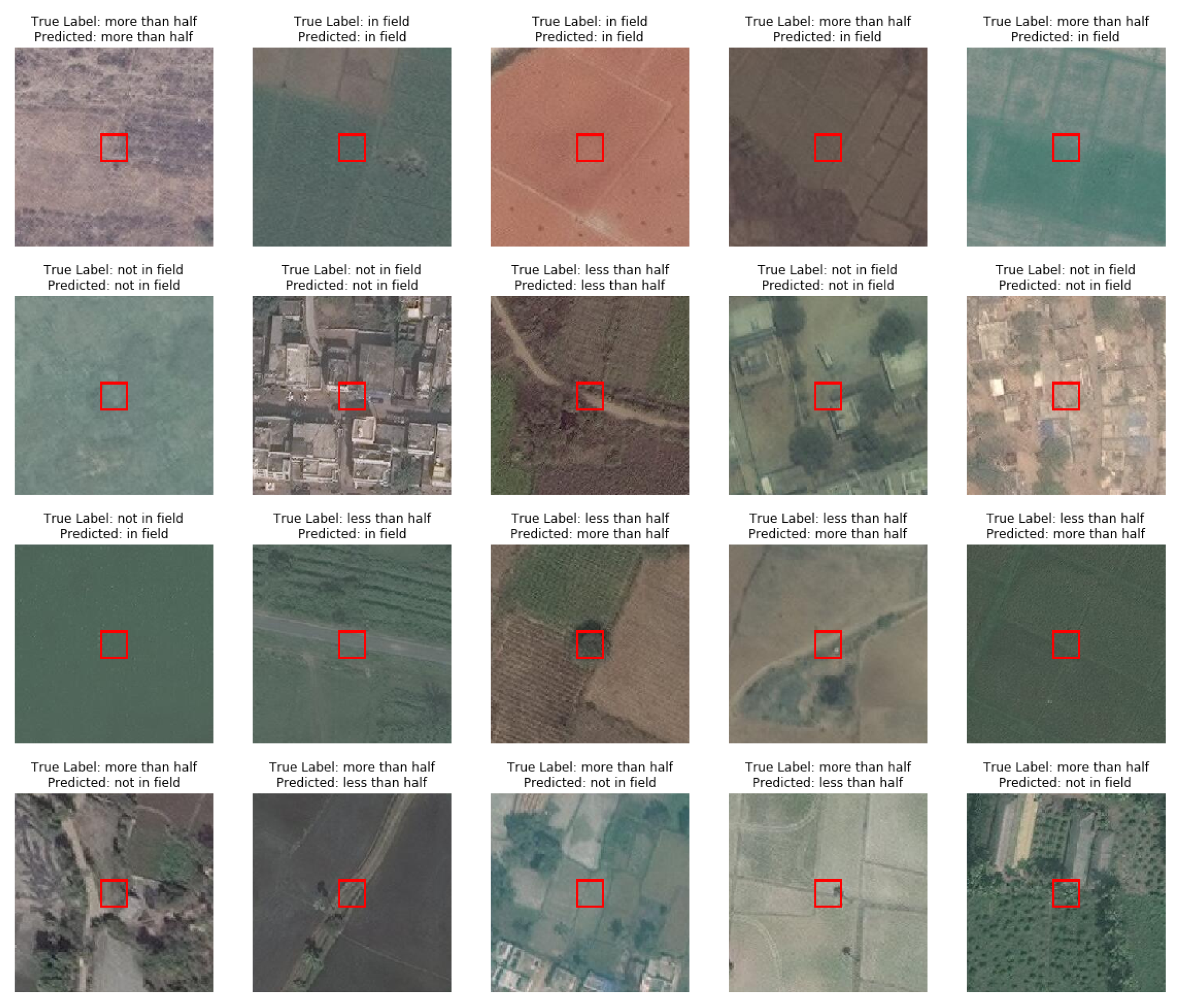
When classification errors occurred, they came mostly from difficulty telling adjacent classes apart, rather than confusing boxes not in a field with those entirely in a field (Figure A6). Grouped together into a binary “more than half” versus “less than half” classification, the corresponding test set accuracy was 89.0%. Examples of correctly and incorrectly classified images are displayed in Figure A7. We see that boxes in urban areas and boxes entirely in rectangular fields were easy to identify as “not in field” and “in field”, respectively, while irregularly-shaped fields, lone trees, and dirt roads occasionally confused the classifier.
We applied the trained ResNet-18 model to predict whether Sentinel-2 pixels are in a field on the remaining submissions without in-field labels, thereby allowing all submissions to be filtered on this attribute. Of the unlabeled submissions, over 55% had Sentinel-2 pixels more than half in a field. These “more than half” in field Sentinel-2 pixels were used to train the crop type classification models.

5.2. Crop Type Classification with Multi-Temporal Satellite Imagery

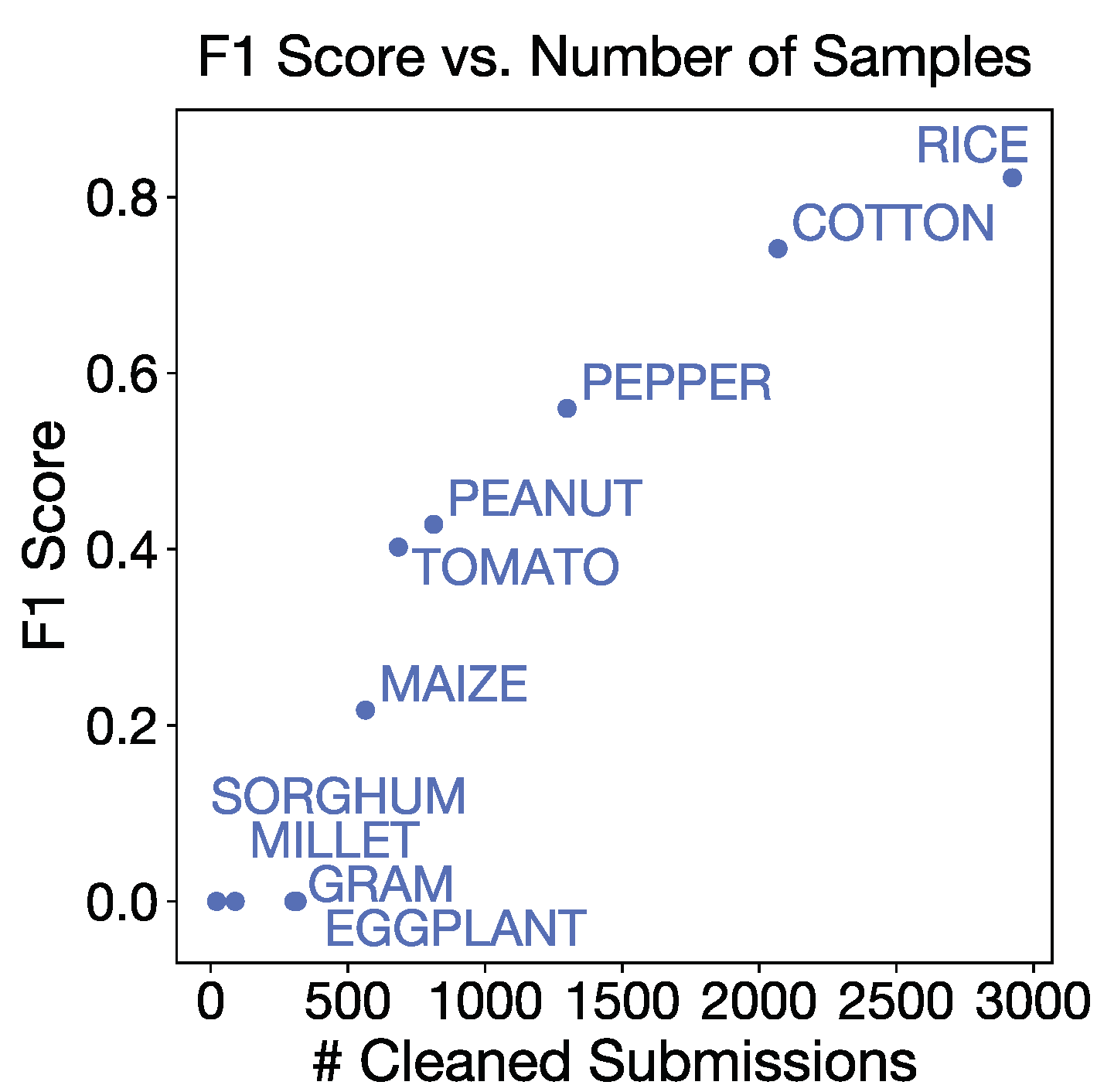
Both neural networks and harmonic coefficients with random forests were able to distinguish rice and cotton from other crops with overall accuracy above 70% (Table 3b); for comparison, a baseline model that classifies everything as the most common class (rice) would achieve 39% accuracy. However, both models struggled to classify minor crops for which there is less data. The 1D CNN, with its highly flexible feature-learning algorithm, consistently outperformed the harmonics and random forest classifier by a small but statistically significant amount (3-class test set accuracy: 74.2 ± 1.4 % CNN versus 71.5 ± 0.7 % harmonics/random forest). On the 10-crop task, however, the recall of non-rice/cotton crops ranged from 20–50% (maize, peanut, pepper, tomato) to 0% (eggplant, gram, millet, and sorghum) (Table 4, full confusion matrix in Figure A13). For all models, the precision and recall were positively correlated with the number of samples available in the training set (Figure 6). The 3D CNN, which has a 21 × 21 -pixel contextualized view of each sample, achieved accuracy lower (3-class task: 72.7%) than the 1D CNN at the cost of much greater data storage and computational runtime (Table A3), which may be due to the much larger number of parameters in the 3D CNN ( 6.1 × 10 6 ) compared to the 1D CNN ( 2.6 × 10 6 ).
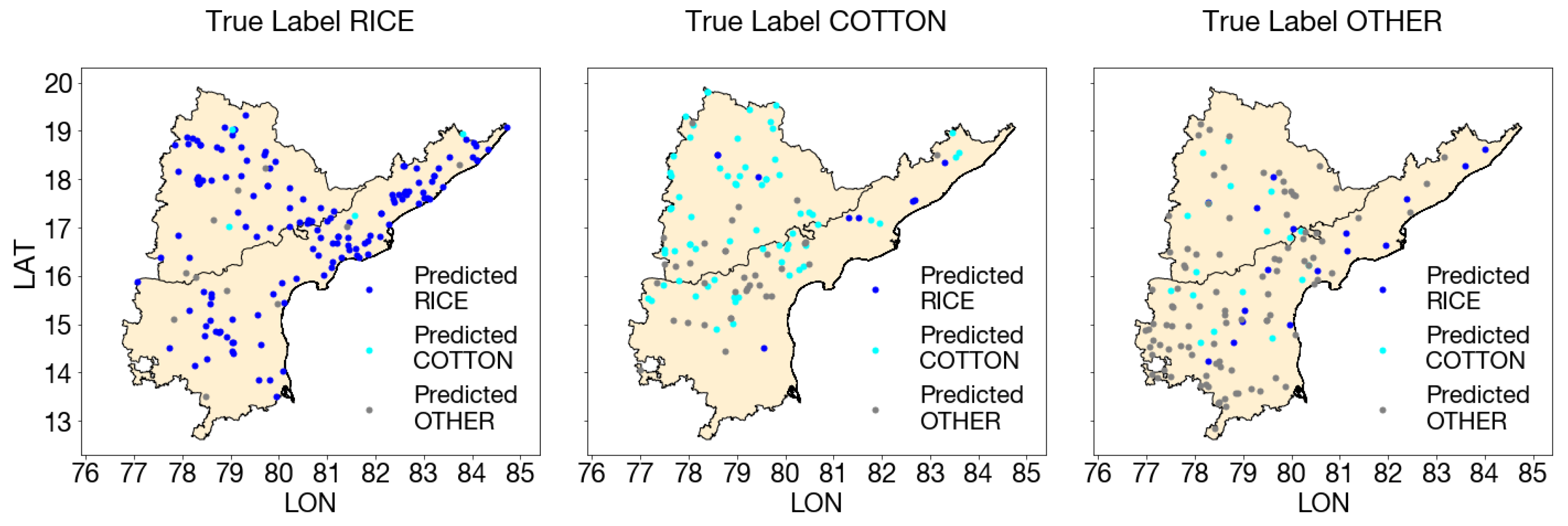
Spatial patterns emerge when we map our crop type predictions against the test set labels. Broadly, rice is common among submissions (and in government statistics) in eastern Andhra Pradesh, cotton in Telangana and northern Andhra Pradesh, and other crops in southwestern Andhra Pradesh. Our models recreate these spatial patterns well (shown for 1D CNN in Figure A14), and are also biased toward these patterns in their errors. For instance, the recall of rice is high in eastern Andhra Pradesh, but at the expense of cotton and other crop recall; rice and other crops misclassified as cotton appear more frequently in Telangana and northern Andhra Pradesh, and misclassified rice and cotton tend to be put in the other class in southwestern Andhra Pradesh. Despite the existence of spatial bias in the model, predictions of all three classes appear throughout the entire study region.

5.3. Combined Sentinel-1 and -2 Imagery Versus Sentinel-2 Only

In our comparison of classification accuracy under models using both Sentinel-1 and -2 imagery versus only Sentinel-2 imagery, we found that adding Sentinel-1 improves performance, especially when features are harmonic coefficients (Table A7). Indeed, on the 3-crop task, adding Sentinel-1 improves overall accuracy on the validation set from 69.4 ± 0.6 % to 75.0 ± 0.8 % when using harmonic features. Permutation experiments also show a number of VV and VH coefficients in the top 30 most important harmonic features (Figure A10). However, the additional value of Sentinel-1 bands on 1D CNN accuracy is not statistically significant relative to the variance introduced by bootstrapping the training set. This may be because the neural network is able to extract more information from the raw Sentinel-2 time series, thereby diminishing the returns from adding Sentinel-1 data. Permutation experiments on the 1D CNN reveal that the neural network relies strongly on the red edge bands (especially around 740 nm, RDED2), short wave infrared, and the difference of VV and VH polarizations (DIFF) to differentiate crop types (Figure 7). This is consistent with prior work showing that red-edge bands are sensitive to leaf and canopy structure [73,74,75] and SWIR bands are sensitive to leaf and soil water content [75,76]. Surprisingly, the VH / VV ratio did not emerge as the top SAR feature despite prior evidence suggesting its sensitivity to crop growth [50]. Instead, the DIFF feature, which is sparsely documented to date, was favored by the model. Permutation of times of year also shows that the most important months to have satellite data are October and November, which correspond to the harvest of kharif crops.

5.4. Robustness to Location and Label Noise

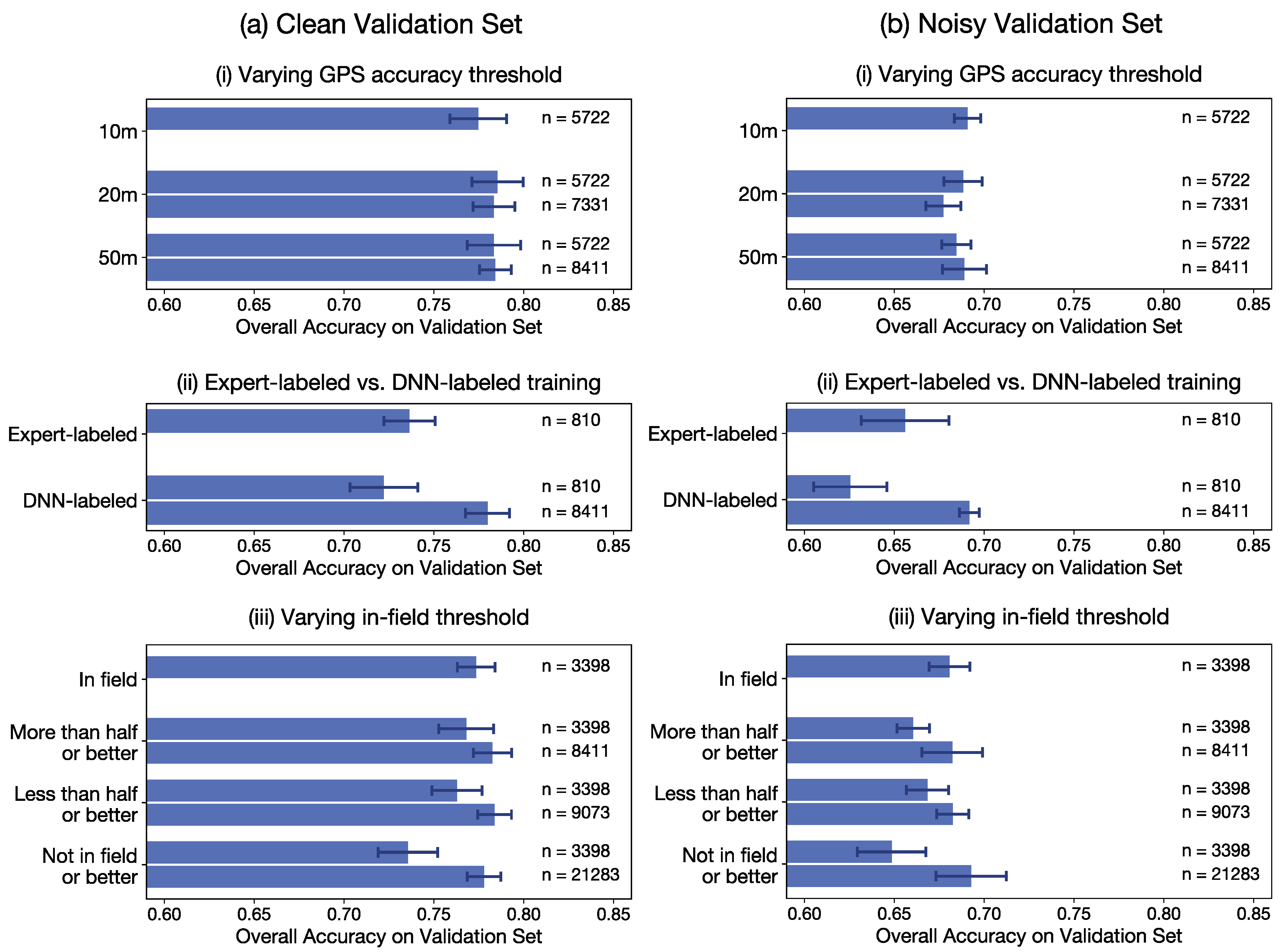
Crowdsourced data can contain many sources of error, and efforts to reduce noise can be costly. To understand whether a noisy Plantix dataset can still be useful for crop type mapping and how much investment should be made to clean it, we tested the sensitivity of 1D CNN performance to both training and validation set quality. Figure 8a shows the effect of increasing training set noise along three axes (GPS accuracy, label origin, and in-field threshold) on a cleaned validation set, while Figure 8b shows the same effects as they appear on a noisy validation set. We use overall accuracy as the metric, but obtained the same analysis for F1 scores.
The conclusions concerning training set quality are similar from both validation sets. First, holding training set sizes constant, training sets with moderate levels of noise did not yield significantly worse validation set accuracies than the highest quality training sets. For example, classifiers trained on samples with GPS locations accurate to 50 m performed as well as those trained on samples with GPS locations accurate to 10 m. Second, adding samples whose labels are noisy to the training set can still boost classification performance. Adding samples labeled by the Plantix-DNN, samples with GPS locations accurate to 50 m, and samples whose Sentinel-2 pixels are only partially in a crop field all increased validation set accuracy (though not to a statistically significant extent in the last two examples). Lastly, high levels of label noise do decrease classification performance, as seen when submissions not in crop fields were added to the training set. However, even in this last setting, validation accuracy degraded only a few percentage points, and the decrease disappeared when all available data was used for training instead of a subsample with the same training set size.
While the CNN is robust to some training set noise, it requires a high quality validation set to yield accurate error estimates on unseen data. Accuracies on the noisy validation set are consistently 10% lower than those on the clean validation set, so that a naive interpretation of results on a noisy validation set would underestimate true classifier performance.

5.5. Comparison to District-Level Data

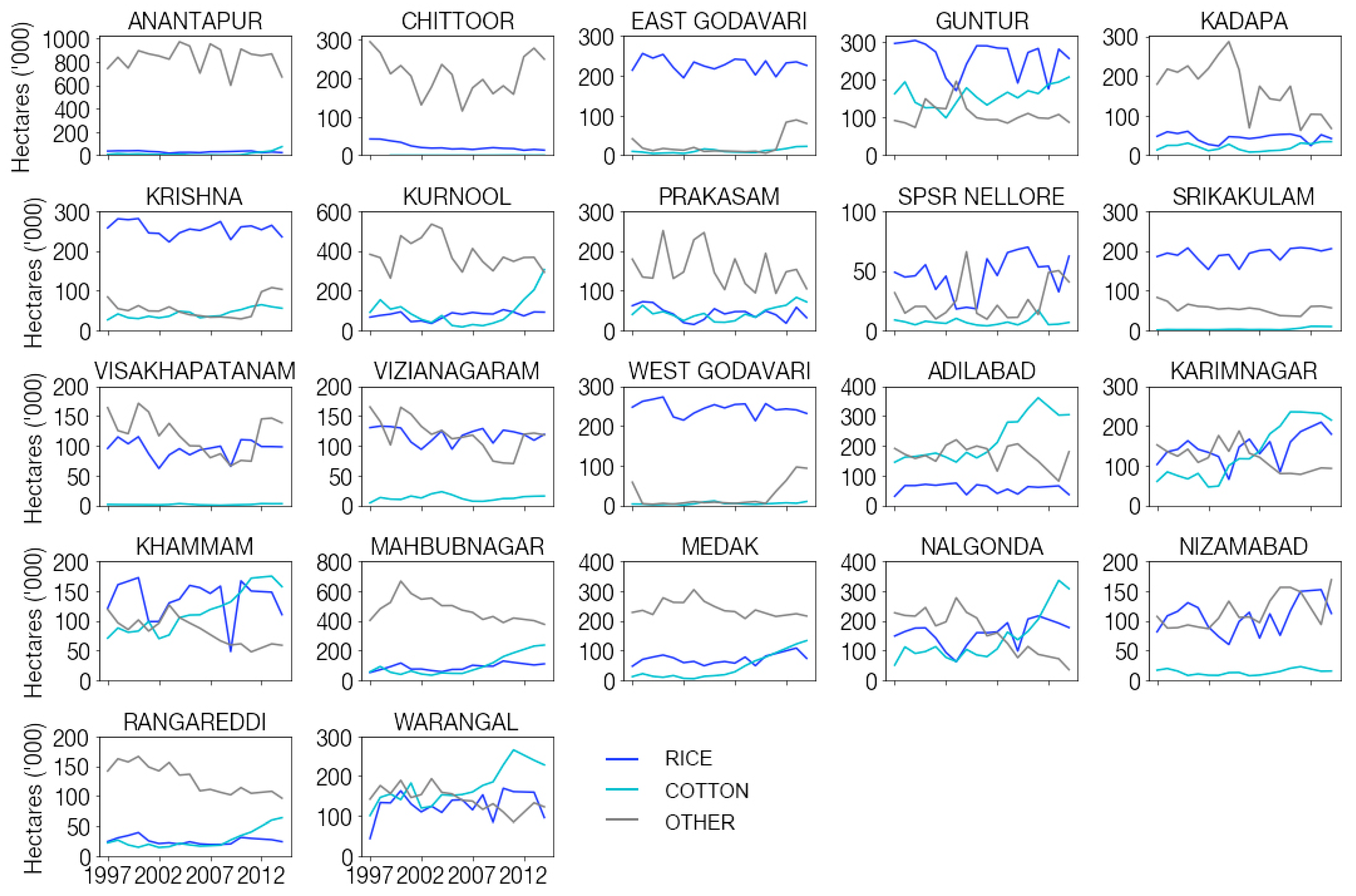
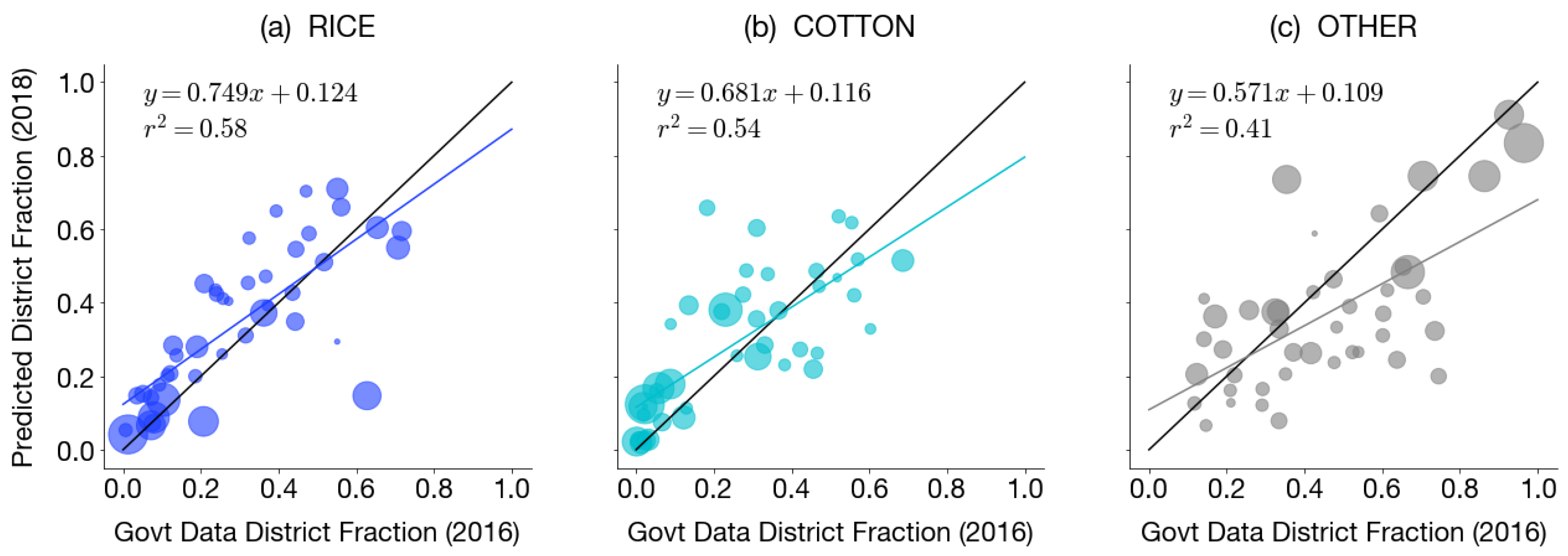
In addition to validating the classifiers on a hold-out set of Plantix submissions, we also compared the 3-class 1D CNN predictions on 2018–2019 GFSAD cropland samples (see Section 4.6) to the 2016–2017 district-level kharif season crop area statistics from the Indian Department of Agriculture [9]. Across 43 districts, R 2 values between the fraction of samples predicted and the fraction of cropped area in the official statistics were 0.58, 0.54, and 0.41 for rice, cotton, and other crops, respectively (Figure 9). The classifier’s aggregated predictions captured broad district-level characteristics correctly—districts like East Godavari, West Godavari, Krishna, and Srikakulam are dominated by rice; Adilabad, Nalgonda, and Warangal are dominated by cotton, and Anantapur and Chittoor grow mostly peanut (groundnut). However, our rice prediction for SPSR Nellore was much lower than the official statistic, and our cotton prediction for Vikarabad was much higher. These discrepancies may be due to a combination of classifier bias, error in the district statistics, and mismatch between the year of our samples and the year of district statistics. Note that comparatively few training samples came from SPSR Nellore (Figure A8), and historical changes in crop area statistics in this district have also been large, suggesting statistics could also have changed between 2016–2017 and 2018–2019 (Figure A18). Meanwhile, cotton dominated training samples in Vikarabad and could have biased the classifier toward predicting cotton on similar time series. While the latitude and longitude of samples were not explicitly provided as features to any classifiers, the 1D CNN could have learned to associate crop type with, say, the satellite image acquisition schedule or regional phenology in addition to with meaningful phenological characteristics. Without more updated district statistics, it is difficult to diagnose the main source of discrepancy between our aggregated predictions and the statistics.

5.6. Study Region-Wide Crop Type Map

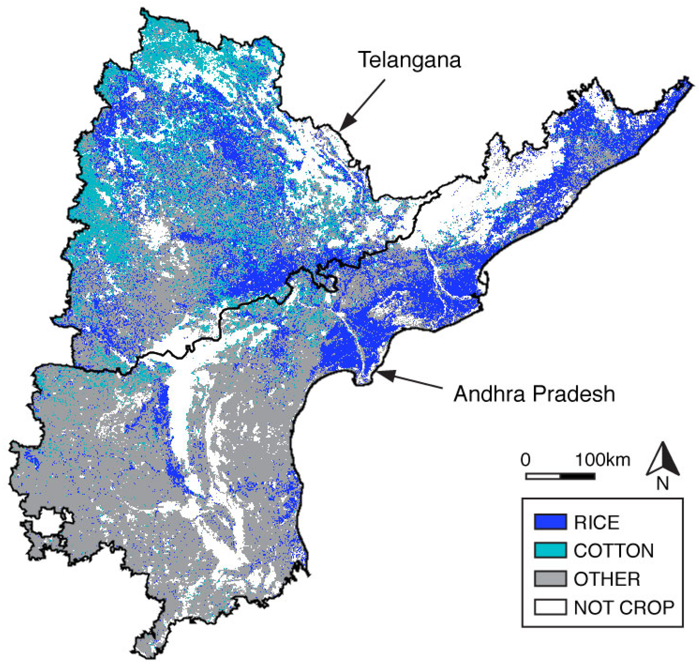
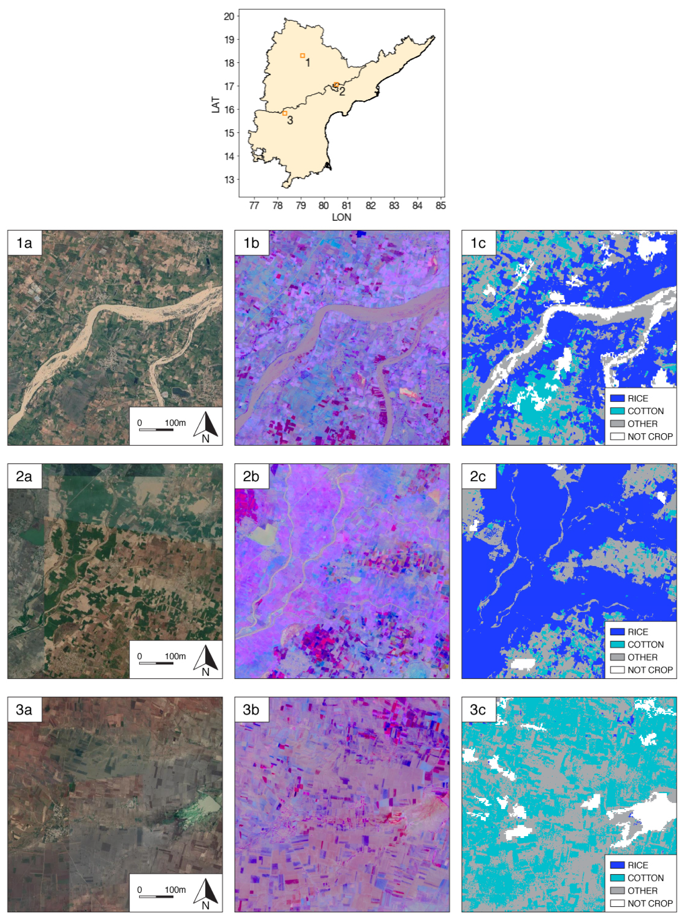
We produced a 10 m ground resolution map of rice, cotton, and other crop across the states of Andhra Pradesh and Telangana for the 2018 kharif season (Figure 10). Three-crop classification performance in Google Earth Engine mirrored the Python performance, achieving 72% accuracy on the held-out test set. The predicted crop type map matches broad patterns of Plantix submission data and government district statistics: rice dominates in the north and northeast regions, cotton dominates in the northwest, and other crops dominate in the south. Sections of the map shown in Figure 11 illustrate these patterns, as well as the frequent prediction of rice along riverbanks. Sources of error in the map include non-cropland regions being classified as cropland and vice versa (from the underlying GFSAD product), and regions with very small field sizes exhibiting high prediction noise. In the latter case, individual pixels differ in prediction from their neighbors, so smoothing techniques may help to address this in future work.
While numerous prior works have mapped paddy rice in South Asia, Plantix labels and Sentinel data enabled us to create a map that is higher resolution than most existing large-scale products, which use MODIS or other medium-resolution imagery and therefore are not at the field level in smallholder systems. An exception is Singha et al. [21], who use Sentinel-1 to map rice in Bangladesh and northeast India and report accuracies exceeding 90%. The crop composition in northeast India is, however, very different from that in AP and Telangana; in the northeast, paddy rice accounts for about 80% of the total cultivated area. Accuracy would therefore appear quite high for a baseline model that assumes all samples are rice. In AP and Telangana, rice is still the most dominant crop but only accounts for 33% of cropped area (according to the government statistics) and comprises 39% of Plantix samples. This highlights that, as more crop type maps are created throughout India and across the world, it can be difficult to compare methodologies and results directly, and one should do so with an understanding of the underlying diversity in cropping systems.

6. Discussion

6.1. Contributions and Shortcomings of This Work

We draw the following lessons from cleaning Plantix submissions to supervise crop classification, which are applicable to both crop type mapping in smallholder systems and land use mapping more generally.
First, crowdsourced data, though very high in noise, can be cleaned and used to supervise remote sensing tasks if data quality is measured for each sample. In this study, location accuracy, whether the submission came from inside a field, and whether crop type was labeled by human experts were important metadata on which to filter Plantix submissions. We discuss the challenges and potential of crowdsourced data in detail in the next section.
Second, a high-quality hold-out set is crucial for assessing model performance accurately. For the same classifier, our results indicate that a higher level of noise in the validation set biases the validation accuracy downward, since the noise is random and follows no learnable pattern. Given that our cleaned validation and test sets still contain non-zero noise, our reported metrics may in fact be underestimates of model performance. At the same time, since conclusions drawn about training set noise sensitivity were similar for both the clean and noisy validation sets, a noisy validation set can still be useful for data filtering and model selection.
Third, classifiers can be robust to noise in the training set—for example, even when a majority of training samples were not in a crop field, the 1D CNN performance degraded only slightly. This observation is consistent with literature on image classification, in which CNNs are found to achieve high classification accuracy even when the training set is scraped from the internet or diluted with 100 noisy labels for each clean label [77,78]. In other words, CNNs can still learn appropriate decision boundaries when trained on highly noisy data. These results suggest that, when researchers face a choice between collecting few high quality labels (usually more expensive per unit) or many noisy labels (cheaper per unit), broader spatial coverage and a larger, more diverse training set are worth trading for moderate decreases in data quality.
Fourth, we tried multiple combinations of Sentinel data and machine learning methods to see whether adding SAR imagery and increasing model capacity could improve crop type mapping. We found that, while the 1D CNN outperforms random forest classifiers, the improvement was modest. Similarly, using Sentinel-1 features slightly improves classification performance over Sentinel-2 features alone. While the recursive harmonics and neural networks show evidence of being somewhat robust to clouds ([18] and Figure A15), the lack of high-quality Sentinel-2 cloud mask remains a weakness of this work and a barrier to global crop type mapping.
The relative performance of random forest, 1D CNN, and 3D CNN suggest that model expressiveness is not the main hindrance to crop type mapping, at least in southeast India. Instead, better features, high quality Sentinel-2 cloud masks, and larger sample sizes are likely needed. The last is especially true for classifying minor crops. While the number of samples required depends on the desired level of accuracy, the quality of satellite imagery, the quality of ground truth labels, the complexity of the agricultural system, and the uniqueness of a crop’s spectral reflectance, the trend in Figure 6 suggests that achieving an F1 score above 0.8 requires at least 3000 cleaned Plantix submissions for training. Future methodological work to map crop types in smallholder systems could focus on leveraging different sensor data, removing clouds, developing data-efficient algorithms, improving classification of minor crop classes, and incorporating prior knowledge to improve classification, rather than more complex, data-hungry supervised learning methods.

6.2. Challenges of Crowdsourced Labels and Possible Ways Forward

The most challenging aspects of working with the Plantix data were (1) high dataset error, which we took measures to reduce, and (2) sampling bias, part of which we mitigated via re-sampling but which largely remained unaddressable post-data collection. Ongoing and future efforts to gather crop type labels via crowdsourcing should consider how to reduce these two sources of error. At the very least, GPS accuracy, location of submission inside a field, and crop label quality must be recorded. Without these measures, high-quality hold-out sets cannot be constructed to accurately assess classifier performance, and low-quality training sets will also degrade classifier performance. We took steps to remove points that had high location uncertainty and were not inside a field to arrive at cleaner subsets of Plantix data. This enabled the training of classifiers that performed much better than a random guessing baseline. Even so, there remains some noise in the cleaned data, as the location accuracy is a probabilistic metric, the in-field classifier has a 10% error rate, and human labelers are also imperfect. Research is needed to further decrease the influence of these sources of noise, and could involve re-weighting the training set based on inferred label accuracy [79], employing noise-tolerant loss functions [80], or adding noise-adaptive layers to the neural network [81].
A second challenge of the Plantix dataset is the sampling bias inherent to using data submitted to an Android application. Farmers had to have internet access and a smartphone to participate in this form of crowdsourcing, while individuals without these resources were systematically excluded from the data. Some of this bias was removed when we re-sampled the dataset to be more geographically uniform; where the raw dataset was heavily concentrated around cities (e.g., Hyberadad), the eventual training, validation, and test sets became more representative of the entire study region. Still, submissions from farmers without access to or knowledge of Plantix are not present in the dataset at all, and, since the agricultural circumstances of this group are likely to differ from those of Plantix users, further work is needed to assess the accuracy of our maps in areas with low mobile internet use.
Taken together, we see that obtaining crowdsourced data that can be used for mapping land use requires nontrivial investments in representative sampling and quality control pre- and post-data collection. For some tasks (e.g., generating crop type or in-field labels), this still entails initial input from experts, albeit at a computer instead of in the field. Once the Plantix submissions were filtered, we were left with 10,000 samples to train a classifier. This is a tiny fraction of total Plantix submissions, and the future of crowdsourcing for label collection depends strongly on increasing the fraction of usable submissions. Some progress in this vein will naturally follow existing technological trends; for example, location accuracy will improve as internet connectivity expands globally. Others, such as in-field classification, require active research.
Despite the large percentage of crowdsourced labels that end up discarded, Plantix has provided more ground data than available previously in similar settings [14,17,18,19] and comparable in volume to the ground truth collected by Indian state agriculture departments annually (11,469 points nationally in kharif and rabi from 2017–2018) [33]. Therefore, despite the challenges of crowdsourcing, the volume and coverage of datasets like Plantix, along with ever-improving data storage, processing, and smartphone access, make crowdsourcing an increasingly viable and useful alternative to traditional field work. In the future, one could imagine combining multiple data collection methods so that validation and test sets are constructed from trusted survey-based methods while large crowdsourced datasets are used to train classifiers. Lastly we note that, while this work focuses on technical feasibility, best practices to preserve data accessibility and privacy will also need to be defined for crowdsourcing to be widely practicable.

7. Conclusions

This is the first study to explore the potential of crowdsourced data to augment or replace ground surveys for land use mapping at a large scale. We derived a large but noisy crowdsourced dataset from the Plantix mobile app to train and validate a crop type map in southeast India. Two million farmer submissions were filtered to 10,000 higher-quality labels, and three machine learning models trained on multi-temporal satellite imagery were able to differentiate rice and cotton from other crops with 70+% accuracy. We found classification performance to be robust to moderate levels of the label and location noise common to crowdsourced data. Our 3-crop prediction (rice, cotton, other) for the 2018 kharif season was validated against a hold-out set of Plantix data and district-level crop area statistics from the Indian Department of Agriculture, and is available upon request.

Author Contributions

Conceptualization, S.W., R.S., and D.B.L.; data curation, J.F., T.F., A.K., and S.W.; methodology, S.W.; software, S.W., J.F., T.F., and S.D.T.; validation, S.W. and S.D.T.; investigation, S.W.; writing—original draft preparation, S.W.; writing—review and editing, S.W., S.D.T., J.F., R.S., and D.B.L.; visualization, S.W.; supervision, D.B.L. and R.S. All authors have read and agreed to the published version of the manuscript.

Funding

This research received no external funding.

Acknowledgments

We thank Christina Sintek for help with data acquisition, Brian Lin for help with data labeling, and Rose Rustowicz and Robin Cheong for sharing software.

Conflicts of Interest

The authors declare no conflict of interest.

Abbreviations

The following abbreviations are used in this manuscript:
APAndhra Pradesh
PEATProgressive Environmental and Agricultural Technologies
GPSGlobal positioning system
SARSynthetic-aperture radar
VVVertical transmit, vertical receive
VHVertical transmit, horizontal receive
DGDigitalGlobe
RGBRed, green, and blue
GFSADGlobal Food Security-support Analysis Data
CNNConvolutional neural network
DNNDeep neural network

Appendix A

Figure A1. Geographic distribution of submissions for each crop type. Crops are ordered by number of submissions in the dataset, rice with the most and sorghum the least.
Remotesensing 12 02957 g0a1
Figure A2. Sentinel-1 time series. For each crop type, VH/VV of Sentinel-1 time series at 5 randomly sampled submissions are shown from 1 April of the crop year to 31 March of the next year.
Remotesensing 12 02957 g0a2
Figure A3. Map of 3000 submissions sampled for “in-field” labeling. The DigitalGlobe image ( 500 × 500 pixels at 0.3 m resolution) centered at each location was downloaded and labeled for whether the center 10 × 10 m box was inside a field.
Remotesensing 12 02957 g0a3
Figure A4. Labeler agreement. Confusion matrix of in-field labels generated by two labelers on a subsample of 200 DigitalGlobe images. Percent agreement across 4 classes is 83%, and across 2 classes (more than half, less than half) is 93%.
Remotesensing 12 02957 g0a4
Figure A5. Pretrained ResNet-18 loss and accuracy across training epochs.
Remotesensing 12 02957 g0a5
Figure A6. In-field classification confusion matrix. Values are shown for test set.
Remotesensing 12 02957 g0a6
Figure A7. From first row to last row: true positives, true negatives, false positives, and false negatives of the binary in-field classification problem. Five examples were sampled at random from each category. The box marks the size of a Sentinel-2 pixel.
Remotesensing 12 02957 g0a7
Figure A8. Maps of Plantix training, validation, and test sets for crop type classification. (a) To build the validation and test sets, we started with the highest quality submissions (GPS accuracy 50 m, more than half of the Sentinel-2 pixel is in a field, crop type was assigned by a human expert). These submissions were highly concentrated in the eastern half of Andhra Pradesh. (b) High quality submissions were re-sampled in a spatially uniform way to form the validation and test sets ( n = 400 for both). (c) The training set was filtered from the remaining dataset to be 500 m away from any points in the validation and test sets, with GPS accuracy 50 m and more than half of the Sentinel-2 pixel in a field.
Remotesensing 12 02957 g0a8
Figure A9. Correlation matrix of harmonic coefficients. The 14 Sentinel-2 bands and 4 Sentinel-1 bands are shown. Within each band, coefficients are shown in order of ascending Fourier frequency, followed by the constant ( a 1 , b 1 , a 2 , b 2 , a 3 , b 3 , c in Equation (1)).
Remotesensing 12 02957 g0a9
Figure A10. Harmonic coefficient feature importance via permutation. The permutation importance is shown for the 30 most important features. Error bars are 1 standard deviation. Fourier terms are shown in inset for reference.
Remotesensing 12 02957 g0a10
Figure A11. 1D CNN architecture.
Remotesensing 12 02957 g0a11
Figure A12. 1D CNN loss and accuracy across training epochs.
Remotesensing 12 02957 g0a12
Figure A13. Crop type classification confusion matrices on the 10-class task and the 3-class task. Values are shown for the test set ( n = 400 ).
Remotesensing 12 02957 g0a13
Figure A14. Map of 1D CNN predictions for rice, cotton, and other kharif crops. From left to right: panels show our model’s predictions for test points whose true labels are rice, cotton, and other, respectively.
Remotesensing 12 02957 g0a14
Figure A15. Occlusion sensitivity analysis. We blocked a 5-day sliding window of values in an example time series and analyzed its effect on the probability score output by the 1D CNN. The time series is originally correctly classified by the network as “rice”. The values substituted in the occlusion window are the mean of the time series. Only GCVI is visualized, but all Sentinel-2 and Sentinel-1 values in the window were occluded. Cloudy observations appear as low values in GCVI. The greater the decrease in log P ( y = RICE ) (more red), the more the 1D CNN relies on that segment of the time series for classification. Conversely, greener segments are less important for classification.
Remotesensing 12 02957 g0a15
Figure A16. 3D CNN architecture.
Remotesensing 12 02957 g0a16
Figure A17. 3D CNN loss and accuracy across training epochs.
Remotesensing 12 02957 g0a17
Figure A18. District-level kharif crop area in Andhra Pradesh and Telangana from 1997–2014. Area data were downloaded from data.gov.in and are shown for rice, cotton, and other, where other shows the sum of non-rice and non-cotton crops.
Remotesensing 12 02957 g0a18
Table A1. Pretrained CNN implementation details. Hyperparameters for the pretrained 2D CNNs used for in-field classification. We refer the reader to references [54,55] for descriptions of the architectures of VGG and ResNet CNNs.
ModelHyperparameterValue
VGG [54]Input size 224 × 224 × 3
Kernel size 3 × 3
Initial filters16
Batch size4
Epochs200
OptimizerSGD
Learning rate0.0001
Momentum0.9
ResNet [55]Input size 224 × 224 × 3
Kernel size 7 × 7 , 3 × 3
Initial filters64
Batch size4
Epochs100
OptimizerAdam
Learning rate0.001
Betas(0.9, 0.999)
AllBrightness jitter0.5
Contrast jitter0.5
Saturation jitter0.5
Hue jitter0
Table A2. In-field model selection. VGG and ResNet training and validation accuracies are shown for 12 architecture and hyperparameter settings. Comparisons to guessing everything is in the majority class (not in field) and human labeler accuracy are provided to gauge task difficulty and lower/upper bounds for metrics. Test accuracy was computed for the model with highest validation accuracy.
ModelLayersGSDBestTrainingValidationTest
L 2 -RegAccuracyAccuracyAccuracy
Majority class0.3880.3680.384
VGG (pretrained)110.3 m0.00.7040.708
0.6 m0.00.7940.730
190.3 m0.00.7270.722
0.6 m0.00.8370.736
ResNet (pretrained)180.3 m0.00.7430.7460.742
0.6 m0.00.7440.716
500.3 m0.00.7220.694
0.6 m0.00.7180.710
VGG
(not pretrained)
110.3 m0.00.7610.722
0.6 m0.00.7200.712
ResNet
(not pretrained)
180.3 m0.00.7700.680
0.6 m0.00.7710.686
Human labeler0.3 m0.8250.8250.825
Table A3. Data storage and computational runtime required of the 3 machine learning algorithms. Data storage is shown for 10,000 samples. Experiment runtimes are shown for the 3-class task for training and validating on a single model. Random forest experiments were performed using sklearn’s RandomForestClassifier with 500 trees on 8 CPUs with 52 GB RAM running Ubuntu 16.04. The CNNs were run on the same machine on one NVIDIA Tesla K80 GPU, and runtimes are shown for 20 epochs.
Harmonics and1D CNN3D CNN
Random Forest
Sentinel-2 data storage27 MB406 MB166 GB
Sentinel-1 data storage8 MB116 MB
Number of parameters 2.6 × 10 6 6.1 × 10 6
Runtime (HH:mm:ss)00:00:4000:02:2244:00:00
Table A4. Harmonics hyperparameter tuning. Grid search was performed to find the best pair of hyperparameters: the number of cosine and sine terms (order) and number of recursive fits. Each combination of hyperparameters was trained with 10 random bootstrapped training sets to obtain error bars (shown for 1 standard deviation). Random forest hyperparameters were kept at default based on previous work [36], except number of trees was increased to 500.
ModelOrderNumberTrainingValidation
of FitsAccuracyAccuracy
Majority class0.3220.399
Harmonic features and random forest21 1.000 ± 0.000 0.739 ± 0.009
2 1.000 ± 0.000 0.741 ± 0.008
4 1.000 ± 0.000 0.735 ± 0.002
8 1.000 ± 0.000 0.734 ± 0.010
16 1.000 ± 0.000 0.734 ± 0.013
31 1.000 ± 0.000 0.746 ± 0.009
2 1.000 ± 0.000 0.750 ± 0.008
4 1.000 ± 0.000 0.726 ± 0.014
8 1.000 ± 0.000 0.728 ± 0.010
16 1.000 ± 0.000 0.708 ± 0.004
41 1.000 ± 0.000 0.748 ± 0.008
2 1.000 ± 0.000 0.749 ± 0.011
4 1.000 ± 0.000 0.740 ± 0.008
8 1.000 ± 0.000 0.722 ± 0.005
16 1.000 ± 0.000 0.721 ± 0.008
Table A5. 1D CNN implementation details. Hyperparameters for the 1D CNN yielding the highest validation set accuracy.
HyperparameterValue
Kernel size3
Conv layers4
Initial filters64
L 2 regularization0.0
Batch size4
OptimizerAdam
Learning rate0.001
Betas(0.9, 0.999)
Table A6. 1D CNN hyperparameter tuning. Due to the large search space, 24 sets of hyperparameters were randomly sampled from the grid of options, and each set was trained with 5 random CNN weight initializations and bootstrapped training sets to obtain error bars (shown for 1 standard deviation).
ModelEncodingLayersInitialLearningBatchTrainingValidation
FiltersRateSizeAccuracyAccuracy
Majority class0.3220.399
1D CNNConstant until updated3160.0014 0.922 ± 0.058 0.672 ± 0.012
640.00014 0.952 ± 0.053 0.683 ± 0.013
480.000116 0.803 ± 0.048 0.764 ± 0.018
0.00116 0.826 ± 0.051 0.783 ± 0.012
320.014 0.435 ± 0.020 0.399 ± 0.000
640.00116 0.802 ± 0.083 0.787 ± 0.010
580.00116 0.797 ± 0.086 0.758 ± 0.014
160.00014 0.754 ± 0.121 0.754 ± 0.006
320.000116 0.966 ± 0.044 0.768 ± 0.016
680.0014 0.722 ± 0.055 0.753 ± 0.010
16 0.782 ± 0.083 0.754 ± 0.008
320.0014 0.660 ± 0.117 0.687 ± 0.144
Zero for missing3160.00014 0.894 ± 0.068 0.632 ± 0.019
640.00014 0.967 ± 0.042 0.662 ± 0.016
480.0014 0.727 ± 0.078 0.757 ± 0.008
580.00014 0.707 ± 0.078 0.750 ± 0.023
320.000116 0.889 ± 0.151 0.757 ± 0.013
0.00116 0.849 ± 0.106 0.763 ± 0.012
0.0116 0.446 ± 0.003 0.399 ± 0.000
640.00116 0.776 ± 0.074 0.760 ± 0.010
680.00116 0.764 ± 0.112 0.755 ± 0.013
320.000116 0.964 ± 0.049 0.758 ± 0.009
640.0014 0.444 ± 0.003 0.399 ± 0.00
0.014 0.446 ± 0.003 0.399 ± 0.00
Table A7. The additional value of Sentinel-1. Training and validation accuracies for the 10-crop classification problem and 3-class problem are compared between models using both SAR and optical (Sentinel-1 and -2) satellite imagery and only optical satellite imagery (Sentinel-2).
ModelNumberSatellite(s)TrainingValidation
of ClassesAccuracyAccuracy
Majority100.3220.399
class30.4500.388
Harmonics + random forest10Sentinel-1 and -2 1.000 ± 0.000 0.629 ± 0.007
Sentinel-2 1.000 ± 0.000 0.611 ± 0.012
3Sentinel-1 and -2 1.000 ± 0.000 0.750 ± 0.008
Sentinel-2 1.000 ± 0.000 0.694 ± 0.006
1D CNN10Sentinel-1 and -2 0.615 ± 0.025 0.645 ± 0.013
Sentinel-2 0.629 ± 0.038 0.636 ± 0.015
3Sentinel-1 and -2 0.802 ± 0.083 0.787 ± 0.010
Sentinel-2 0.754 ± 0.014 0.775 ± 0.008

References

  1. Khalil, C.A.; Conforti, P.; Ergin, I.; Gennari, P. Defining Small Scale Food Producers to Monitor Target 2.3. of the 2030 Agenda for Sustainable Development; Technical Report; Food and Agriculture Organization of the United Nations: Rome, Italy, 2017. [Google Scholar]
  2. Lowder, S.K.; Skoet, J.; Raney, T. The Number, Size, and Distribution of Farms, Smallholder Farms, and Family Farms Worldwide. World Dev. 2016, 87, 16–29. [Google Scholar] [CrossRef] [Green Version]
  3. Rapsomanikis, G. The Economic Lives of Smallholder Farmers; Technical Report; Food and Agriculture Organization of the United Nations: Rome, Italy, 2015. [Google Scholar] [CrossRef]
  4. Ricciardi, V.; Ramankutty, N.; Mehrabi, Z.; Jarvis, L.; Chookolingo, B. How much of the world’s food do smallholders produce? Glob. Food Secur. 2018, 17, 64–72. [Google Scholar] [CrossRef]
  5. Samberg, L.H.; Gerber, J.S.; Ramankutty, N.; Herrero, M.; West, P.C. Subnational distribution of average farm size and smallholder contributions to global food production. Environ. Res. Lett. 2016, 11, 124010. [Google Scholar] [CrossRef]
  6. Burke, M.; Lobell, D.B. Satellite-based assessment of yield variation and its determinants in smallholder African systems. Proc. Natl. Acad. Sci. USA 2017, 114, 2189–2194. [Google Scholar] [CrossRef] [Green Version]
  7. Plourde, J.D.; Pijanowski, B.C.; Pekin, B.K. Evidence for increased monoculture cropping in the Central United States. Agric. Ecosyst. Environ. 2013, 165, 50–59. [Google Scholar] [CrossRef]
  8. Espey, J. Data for Development: A Needs Assessment for SDG Monitoring and Statistical Capacity Development; Technical Report; Sustainable Development Solutions Network: New York, NY, USA, 2015. [Google Scholar]
  9. Ministry of Agriculture and Farmers’ Welfare. Crop Production Statistics Information System. 2017. Available online: https://aps.dac.gov.in/APY/Index.htm (accessed on 28 September 2019).
  10. Christiaensen, L. Agriculture in Africa—Telling myths from facts: A synthesis. Food Policy 2017, 67, 1–11. [Google Scholar] [CrossRef]
  11. Atzberger, C. Advances in Remote Sensing of Agriculture: Context Description, Existing Operational Monitoring Systems and Major Information Needs. Remote Sens. 2013, 5, 949–981. [Google Scholar] [CrossRef] [Green Version]
  12. USDA National Agricultural Statistics Service Cropland Data Layer. Published Crop-Specific Data Layer [Online]. 2018. Available online: https://nassgeodata.gmu.edu/CropScape/ (accessed on 29 August 2019).
  13. Fisette, T.; Rollin, P.; Aly, Z.; Campbell, L.; Daneshfar, B.; Filyer, P.; Smith, A.; Davidson, A.; Shang, J.; Jarvis, I. AAFC annual crop inventory. In Proceedings of the 2013 Second International Conference on Agro-Geoinformatics (Agro-Geoinformatics), Fairfax, VA, USA, 12–16 August 2013; pp. 270–274. [Google Scholar] [CrossRef]
  14. Inglada, J.; Arias, M.; Tardy, B.; Hagolle, O.; Valero, S.; Morin, D.; Dedieu, G.; Sepulcre, G.; Bontemps, S.; Defourny, P.; et al. Assessment of an Operational System for Crop Type Map Production Using High Temporal and Spatial Resolution Satellite Optical Imagery. Remote Sens. 2015, 7, 12356–12379. [Google Scholar] [CrossRef] [Green Version]
  15. Kremen, C.; Iles, A.; Bacon, C. Diversified Farming Systems: An Agroecological, Systems-based Alternative to Modern Industrial Agriculture. Ecol. Soc. 2012, 17, 44. [Google Scholar] [CrossRef]
  16. Sheahan, M.; Barrett, C.B. Ten striking facts about agricultural input use in Sub-Saharan Africa. Food Policy 2017, 67, 12–25. [Google Scholar] [CrossRef] [Green Version]
  17. Defourny, P.; Bontemps, S.; Bellemans, N.; Cara, C.; Dedieu, G.; Guzzonato, E.; Hagolle, O.; Inglada, J.; Nicola, L.; Rabaute, T.; et al. Near real-time agriculture monitoring at national scale at parcel resolution: Performance assessment of the Sen2-Agri automated system in various cropping systems around the world. Remote Sens. Environ. 2019, 221, 551–568. [Google Scholar] [CrossRef]
  18. Jin, Z.; Azzari, G.; You, C.; Tommaso, S.D.; Aston, S.; Burke, M.; Lobell, D.B. Smallholder maize area and yield mapping at national scales with Google Earth Engine. Remote Sens. Environ. 2019, 228, 115–128. [Google Scholar] [CrossRef]
  19. Singh, R.P.; Sridhar, V.N.; Dadhwal, V.K.; Jaishankar, R.; Neelkanthan, M.; Srivastava, A.K.; Bairagi, G.D.; Sharma, N.K.; Raza, S.A.; Sharma, R.; et al. Village level crop inventory using remote sensing and field survey data. J. Indian Soc. Remote Sens. 2005, 33, 93–98. [Google Scholar] [CrossRef]
  20. Xiao, X.; Dorovskoy, P.; Biradar, C.; Bridge, E. A library of georeferenced photos from the field. EOS Trans. Am. Geophys. Union 2011, 92, 453–454. [Google Scholar] [CrossRef]
  21. Singha, M.; Dong, J.; Zhang, G.; Xiao, X. High resolution paddy rice maps in cloud-prone Bangladesh and Northeast India using Sentinel-1 data. Sci. Data 2019, 6, 26. [Google Scholar] [CrossRef]
  22. Son, N.T.; Chen, C.F.; Chen, C.R.; Duc, H.N.; Chang, L.Y. A Phenology-Based Classification of Time-Series MODIS Data for Rice Crop Monitoring in Mekong Delta, Vietnam. Remote Sens. 2014, 6, 135–156. [Google Scholar] [CrossRef] [Green Version]
  23. Mondal, S.; Jeganathan, C.; Sinha, N.K.; Rajan, H.; Roy, T.; Kumar, P. Extracting seasonal cropping patterns using multi-temporal vegetation indices from IRS LISS-III data in Muzaffarpur District of Bihar, India. Egypt. J. Remote Sens. Space Sci. 2014, 17, 123–134. [Google Scholar] [CrossRef] [Green Version]
  24. Xiao, X.; Boles, S.; Frolking, S.; Li, C.; Babu, J.Y.; Salas, W.; Moore, B. Mapping paddy rice agriculture in South and Southeast Asia using multi-temporal MODIS images. Remote Sens. Environ. 2006, 100, 95–113. [Google Scholar] [CrossRef]
  25. Ambika, A.K.; Wardlow, B.; Mishra, V. Remotely sensed high resolution irrigated area mapping in India for 2000 to 2015. Sci. Data 2016, 3, 160118. [Google Scholar] [CrossRef] [Green Version]
  26. Gumma, M.K.; Thenkabail, P.S.; Teluguntla, P.; Rao, M.N.; Mohammed, I.A.; Whitbread, A.M. Mapping rice-fallow cropland areas for short-season grain legumes intensification in South Asia using MODIS 250 m time-series data. Int. J. Digit. Earth 2016, 9, 981–1003. [Google Scholar] [CrossRef] [Green Version]
  27. Manjunath, K.; More, R.S.; Jain, N.; Panigrahy, S.; Parihar, J. Mapping of rice-cropping pattern and cultural type using remote-sensing and ancillary data: A case study for South and Southeast Asian countries. Int. J. Remote Sens. 2015, 36, 6008–6030. [Google Scholar] [CrossRef]
  28. Ministry of Agriculture and Farmers’ Welfare, Government of India. All India Report on Number and Area of Operational Holdings 2015–2016; Ministry of Agriculture and Farmers’ Welfare, Government of India: New Delhi, India, 2019.
  29. Parida, B.R.; Ranjan, A.K. Wheat Acreage Mapping and Yield Prediction Using Landsat-8 OLI Satellite Data: A Case Study in Sahibganj Province, Jharkhand (India). Remote Sens. Earth Syst. Sci. 2019, 2, 96–107. [Google Scholar] [CrossRef]
  30. Misra, G.; Kumar, A.; Patel, N.R.; Zurita-Milla, R. Mapping a Specific Crop—A Temporal Approach for Sugarcane Ratoon. J. Indian Soc. Remote Sens. 2014, 42, 325–334. [Google Scholar] [CrossRef]
  31. Dubey, S.K.; Gavli, A.S.; Yadav, S.K.; Sehgal, S.; Ray, S.S. Remote Sensing-Based Yield Forecasting for Sugarcane (Saccharum officinarum L.) Crop in India. J. Indian Soc. Remote Sens. 2018, 46, 1823–1833. [Google Scholar] [CrossRef]
  32. Internet and Mobile Association of India. Mobile Internet Report 2017; Technical Report, Kantar IMRB; Internet and Mobile Association of India: Mumbai, India, 2018. [Google Scholar]
  33. FASAL (Forecasting Agricultural Output Using Space, Agro-Meteorology and Land Based Observations). 2019. Available online: http://www.ncfc.gov.in/about_fasal.html (accessed on 24 September 2019).
  34. Ghazaryan, G.; Dubovyk, O.; Löw, F.; Lavreniuk, M.; Kolotii, A.; Schellberg, J.; Kussul, N. A rule-based approach for crop identification using multi-temporal and multi-sensor phenological metrics. Eur. J. Remote Sens. 2018, 51, 511–524. [Google Scholar] [CrossRef]
  35. Jakubauskas, M.E.; Legates, D.R.; Kastens, J.H. Crop identification using harmonic analysis of time-series AVHRR NDVI data. Comput. Electron. Agric. 2002, 37, 127–139. [Google Scholar] [CrossRef]
  36. Wang, S.; Azzari, G.; Lobell, D.B. Crop type mapping without field-level labels: Random forest transfer and unsupervised clustering techniques. Remote Sens. Environ. 2019, 222, 303–317. [Google Scholar] [CrossRef]
  37. Breiman, L. Random Forests. Mach. Learn. 2001, 45, 5–32. [Google Scholar] [CrossRef] [Green Version]
  38. LeCun, Y.; Bengio, Y.; Hinton, G. Deep learning. Nature 2015, 521, 436. [Google Scholar] [CrossRef]
  39. Prasuna, V.V.L.; Suneetha, B.; Madhavi, K.; Haritha, G.V.; Murthy, G.R.R. Irrigation status, issues and management in Andhra Pradesh. Ground Water 2018, 1532, 1–42. [Google Scholar]
  40. Forest Survey of India. State of Forest Report 2017; Technical Report; Ministry of Environment and Forests, Government of India: New Delhi, India, 2018.
  41. Useya, J.; Chen, S. Exploring the Potential of Mapping Cropping Patterns on Smallholder Scale Croplands Using Sentinel-1 SAR Data. Chin. Geogr. Sci. 2019, 29, 626–639. [Google Scholar] [CrossRef] [Green Version]
  42. SNAP—Sentinel Application Platform. Available online: http://step.esa.int/main/toolboxes/snap/ (accessed on 22 August 2020).
  43. Rumora, L.; Miler, M.; Medak, D. Contemporary comparative assessment of atmospheric correction influence on radiometric indices between Sentinel-2A and Landsat 8 imagery. Geocarto Int. 2019, 1–15. [Google Scholar] [CrossRef]
  44. Rumora, L.; Miler, M.; Medak, D. Impact of Various Atmospheric Corrections on Sentinel-2 Land Cover Classification Accuracy Using Machine Learning Classifiers. ISPRS Int. J. Geo-Inf. 2020, 9, 277. [Google Scholar] [CrossRef] [Green Version]
  45. Gorelick, N.; Hancher, M.; Dixon, M.; Ilyushchenko, S.; Thau, D.; Moore, R. Google Earth Engine: Planetary-scale geospatial analysis for everyone. Remote Sens. Environ. 2017, 202, 18–27. [Google Scholar] [CrossRef]
  46. Gitelson, A.A.; Vina, A.; Ciganda, V.; Rundquist, D.C.; Arkebauer, T.J. Remote estimation of canopy chlorophyll content in crops. Geophys. Res. Lett. 2005, 32. [Google Scholar] [CrossRef] [Green Version]
  47. Nguy-Robertson, A.L.; Peng, Y.; Gitelson, A.A.; Arkebauer, T.J.; Pimstein, A.; Herrmann, I.; Karnieli, A.; Rundquist, D.C.; Bonfil, D.J. Estimating green LAI in four crops: Potential of determining optimal spectral bands for a universal algorithm. Agric. For. Meteorol. 2014, 192–193, 140–148. [Google Scholar] [CrossRef]
  48. Jain, M.; Srivastava, A.K.; Balwinder-Singh; Joon, R.K.; McDonald, A.; Royal, K.; Lisaius, M.C.; Lobell, D.B. Mapping Smallholder Wheat Yields and Sowing Dates Using Micro-Satellite Data. Remote Sens. 2016, 8, 860. [Google Scholar] [CrossRef] [Green Version]
  49. Coluzzi, R.; Imbrenda, V.; Lanfredi, M.; Simoniello, T. A first assessment of the Sentinel-2 Level 1-C cloud mask product to support informed surface analyses. Remote Sens. Environ. 2018, 217, 426–443. [Google Scholar] [CrossRef]
  50. Veloso, A.; Mermoz, S.; Bouvet, A.; Toan, T.L.; Planells, M.; Dejoux, J.F.; Ceschia, E. Understanding the temporal behavior of crops using Sentinel-1 and Sentinel-2-like data for agricultural applications. Remote Sens. Environ. 2017, 199, 415–426. [Google Scholar] [CrossRef]
  51. Laurin, G.V.; Balling, J.; Corona, P.; Mattioli, W.; Papale, D.; Puletti, N.; Rizzo, M.; Truckenbrodt, J.; Urban, M. Above-ground biomass prediction by Sentinel-1 multitemporal data in central Italy with integration of ALOS2 and Sentinel-2 data. J. Appl. Remote Sens. 2018, 12, 016008. [Google Scholar] [CrossRef]
  52. Dasari, K.; Anjaneyulu, L.; Jayasri, P.V.; Prasad, A.V.V. Importance of speckle filtering in image classification of SAR data. In Proceedings of the 2015 International Conference on Microwave, Optical and Communication Engineering (ICMOCE), Bhubaneswar, India, 18–20 December 2015; pp. 349–352. [Google Scholar]
  53. Ministry of Agriculture and Farmers’ Welfare. District-Wise, Season-Wise Crop Production Statistics. 2015. Available online: https://data.gov.in/catalog/district-wise-season-wise-crop-production-statistics (accessed on 1 September 2019).
  54. Simonyan, K.; Zisserman, A. Very Deep Convolutional Networks for Large-Scale Image Recognition. arXiv 2014, arXiv:1409.1556. [Google Scholar]
  55. He, K.; Zhang, X.; Ren, S.; Sun, J. Deep Residual Learning for Image Recognition. arXiv 2015, arXiv:1512.03385. [Google Scholar]
  56. Marmanis, D.; Datcu, M.; Esch, T.; Stilla, U. Deep Learning Earth Observation Classification Using ImageNet Pretrained Networks. IEEE Geosci. Remote Sens. Lett. 2016, 13, 105–109. [Google Scholar] [CrossRef] [Green Version]
  57. Paszke, A.; Gross, S.; Chintala, S.; Chanan, G.; Yang, E.; DeVito, Z.; Lin, Z.; Desmaison, A.; Antiga, L.; Lerer, A. Automatic Differentiation in PyTorch. OpenReview, 28 October 2017. [Google Scholar]
  58. European Space Agency. Sentinel-2 MSI Data Product Quality Report. July 2018. Available online: https://sentinels.copernicus.eu/web/sentinel/data-product-quality-reports (accessed on 19 July 2020).
  59. Shumway, R.H.; Stoffer, D.S. Time Series Analysis and Its Applications (Springer Texts in Statistics); Springer: Berlin/Heidelberg, Germany, 2005. [Google Scholar]
  60. Jönsson, P.; Eklundh, L. TIMESAT—A program for analyzing time-series of satellite sensor data. Comput. Geosci. 2004, 30, 833–845. [Google Scholar] [CrossRef] [Green Version]
  61. Gislason, P.O.; Benediktsson, J.A.; Sveinsson, J.R. Random Forests for land cover classification. Pattern Recognit. Lett. 2006, 27, 294–300. [Google Scholar] [CrossRef]
  62. Azzari, G.; Lobell, D. Landsat-based classification in the cloud: An opportunity for a paradigm shift in land cover monitoring. Remote Sens. Environ. 2017, 202, 64–74. [Google Scholar] [CrossRef]
  63. Ok, A.O.; Akar, O.; Gungor, O. Evaluation of random forest method for agricultural crop classification. Eur. J. Remote Sens. 2012, 45, 421–432. [Google Scholar] [CrossRef]
  64. Gomez, C.; White, J.C.; Wulder, M.A. Optical remotely sensed time series data for land cover classification: A review. ISPRS J. Photogramm. Remote Sens. 2016, 116, 55–72. [Google Scholar] [CrossRef] [Green Version]
  65. Pedregosa, F.; Varoquaux, G.; Gramfort, A.; Michel, V.; Thirion, B.; Grisel, O.; Blondel, M.; Prettenhofer, P.; Weiss, R.; Dubourg, V.; et al. Scikit-learn: Machine Learning in Python. J. Mach. Learn. Res. 2011, 12, 2825–2830. [Google Scholar]
  66. Che, Z.; Purushotham, S.; Cho, K.; Sontag, D.; Liu, Y. Recurrent Neural Networks for Multivariate Time Series with Missing Values. Sci. Rep. 2018, 8, 6085. [Google Scholar] [CrossRef] [Green Version]
  67. Zeiler, M.D.; Fergus, R. Visualizing and Understanding Convolutional Networks. In Proceedings of the Computer Vision—ECCV 2014, Zurich, Switzerland, 6–12 September 2014; Fleet, D., Pajdla, T., Schiele, B., Tuytelaars, T., Eds.; Springer International Publishing: Cham, Switzerland, 2014; pp. 818–833. [Google Scholar]
  68. Zhou, B.; Khosla, A.; Lapedriza, A.; Oliva, A.; Torralba, A. Learning Deep Features for Discriminative Localization. In Proceedings of the 2016 Conference on Computer Vision and Pattern Recognition (CVPR 2016), Las Vegas, NV, USA, 26 June–1 July 2016. [Google Scholar]
  69. Selvaraju, R.R.; Cogswell, M.; Das, A.; Vedantam, R.; Parikh, D.; Batra, D. Grad-CAM: Visual Explanations from Deep Networks via Gradient-Based Localization. In Proceedings of the 2017 IEEE International Conference on Computer Vision (ICCV), Venice, Italy, 22–29 October 2017; pp. 618–626. [Google Scholar]
  70. Rußwurm, M.; Körner, M. Multi-Temporal Land Cover Classification with Sequential Recurrent Encoders. ISPRS Int. J. Geo-Inf. 2018, 7, 129. [Google Scholar] [CrossRef] [Green Version]
  71. Ronneberger, O.; Fischer, P.; Brox, T. U-Net: Convolutional Networks for Biomedical Image Segmentation. In Proceedings of the Medical Image Computing and Computer-Assisted Intervention—MICCAI 2015, Munich, Germany, 5–9 October 2015; Navab, N., Hornegger, J., Wells, W.M., Frangi, A.F., Eds.; Springer International Publishing: Cham, Switzerland, 2015; pp. 234–241. [Google Scholar]
  72. Gumma, M.K.; Thenkabail, P.S.; Teluguntla, P.; Oliphant, A.J.; Xiong, J.; Congalton, R.G.; Yadav, K.; Phalke, A.; Smith, C. NASA Making Earth System Data Records for Use in Research Environments (MEaSUREs) Global Food Security-Support Analysis Data (GFSAD) Cropland Extent 2015 South Asia, Afghanistan, Iran 30 m V001 [Data Set]. 2017. Available online: https://doi.org/10.5067/MEaSUREs/GFSAD/GFSAD30SAAFGIRCE.001 (accessed on 24 September 2019).
  73. Forkuor, G.; Dimobe, K.; Serme, I.; Tondoh, J.E. Landsat-8 vs. Sentinel-2: Examining the added value of Sentinel-2’s red-edge bands to land-use and land-cover mapping in Burkina Faso. GIScience Remote Sens. 2018, 55, 331–354. [Google Scholar] [CrossRef]
  74. Ustuner, M.; Balik Sanli, F.; Abdikan, S.; Esetlili, M.; Kurucu, Y. Crop Type Classification Using Vegetation Indices of RapidEye Imagery. Int. Arch. Photogramm. Remote. Sens. Spat. Inf. Sci. 2014, 40, 195. [Google Scholar] [CrossRef] [Green Version]
  75. Radoux, J.; Chomé, G.; Jacques, D.C.; Waldner, F.; Bellemans, N.; Matton, N.; Lamarche, C.; D’Andrimont, R.; Defourny, P. Sentinel-2’s Potential for Sub-Pixel Landscape Feature Detection. Remote Sens. 2016, 8, 488. [Google Scholar] [CrossRef] [Green Version]
  76. Immitzer, M.; Vuolo, F.; Atzberger, C. First Experience with Sentinel-2 Data for Crop and Tree Species Classifications in Central Europe. Remote Sens. 2016, 8, 166. [Google Scholar] [CrossRef]
  77. Rolnick, D.; Veit, A.; Belongie, S.; Shavit, N. Deep Learning is Robust to Massive Label Noise. arXiv 2017, arXiv:cs.LG/1705.10694. [Google Scholar]
  78. Krause, J.; Sapp, B.; Howard, A.; Zhou, H.; Toshev, A.; Duerig, T.; Philbin, J.; Fei-Fei, L. The Unreasonable Effectiveness of Noisy Data for Fine-Grained Recognition. In Proceedings of the Computer Vision—ECCV 2016, Amsterdam, The Netherlands, 8–16 October 2016; Leibe, B., Matas, J., Sebe, N., Welling, M., Eds.; Springer International Publishing: Cham, Switzerland, 2016; pp. 301–320. [Google Scholar]
  79. Liu, T.; Tao, D. Classification with Noisy Labels by Importance Reweighting. IEEE Trans. Pattern Anal. Mach. Intell. 2016, 38, 447–461. [Google Scholar] [CrossRef] [Green Version]
  80. Ghosh, A.; Kumar, H.; Sastry, P.S. Robust Loss Functions under Label Noise for Deep Neural Networks. In Proceedings of the Thirty-First AAAI Conference on Artificial Intelligence, San Francisco, CA, USA, 4–10 February 2017; pp. 1919–1925. [Google Scholar]
  81. Goldberger, J.; Ben-Reuven, E. Training deep neural-networks using a noise adaptation layer. In Proceedings of the ICLR 2017, Toulon, France, 24–26 April 2017. [Google Scholar]
Figure 1. Map and submission times of Plantix dataset. (a) Geographic distribution of farmer submissions for rice, cotton, pepper, and peanut. These four crops have the most Plantix submissions within the states of Andhra Pradesh and Telangana (for maps of all ten crop types, see Figure A1 ). (b) Farmer submissions per day from 1 April 2017 to 31 December 2019 for the same four crops.
Remotesensing 12 02957 g001
Figure 2. Raw Sentinel-2 time series. For each crop type, the green chlorophyll vegetation index (GCVI) of Sentinel-2 time series at 5 randomly sampled submissions are shown from 1 April of the crop year to 31 March of the next year. GCVI is defined as NIR / green 1 and measures chlorophyll concentration in vegetation.
Remotesensing 12 02957 g002
Figure 3. Explanatory diagram of the methods presented in this paper. Raw datasets are shown on the left; the data are cleaned and input to feature extraction and machine learning models, and the methods output crop type predictions that are validated against both a hold-out set of ground labels and government statistics on crop area.
Remotesensing 12 02957 g003
Figure 4. Sources of error in crowdsourced locations and crop type labels. (a) Android location accuracy varies from 1 m to 10 km depending on battery life preservation. Histogram shows accuracy distribution with 50 m as cutoff for inclusion in our analyses. (b) Sentinel-2 pixel (denoted by 10 × 10 m white box) may range from entirely inside to entirely not inside a crop field. (c) Plantix photo-based deep convolutional neural network (DNN) crop type prediction is imperfect and varies by crop type. (d) Clustered submissions from active locations overrepresent some geographic subregions.
Remotesensing 12 02957 g004
Figure 5. Feature extraction methods for Sentinel-2 time series. For the same example rice submission, (a) third-order harmonic regression with six recursive fits, (b) 1D convolutional neural network (CNN) time series input, and (c) 3D CNN time series schematic for an entire tile surrounding the submission are shown for the green chlorophyll vegetation index (GCVI) band. In (b,c), days without a Sentinel-2 image are filled in with the most recent previous image. In (c), the yellow box encircles the labeled submission pixel; all other pixels are unlabeled.
Remotesensing 12 02957 g005
Figure 6. F1 score versus training set size by crop type. Precision and recall from Table 4 are summarized as one F1 score for each crop type.
Remotesensing 12 02957 g006
Figure 7. CNN feature importance. Importance was computed as the decrease in validation set accuracy when the feature was permuted across samples, breaking the association between the feature and the label. For the 1D CNN, permuted features were (a) optical and SAR bands and (b) times of year. Error bars were obtained over 10 runs with 10 different bootstrapped training sets.
Remotesensing 12 02957 g007
Figure 8. Sensitivity of classification results to dataset noise. The effect of increasing label error is shown along three dimensions of noise: GPS accuracy threshold (10 m, 20 m, 50 m), label source (expert vs. DNN), and in-field threshold (in field, more than half, less than half, and not in field) for (a) a clean validation set and (b) a noisy validation set.
Remotesensing 12 02957 g008
Figure 9. Comparison of model predictions (y axis) to government statistics (x axis). Results are shown for (a) rice, (b) cotton, and (c) other crops of the 2018–2019 kharif season. Predictions and r 2 values are based on a random sample of cropland from the GFSAD product [72] on which Sentinel-1 and -2 features were extracted and run through the 1D CNN. The black line shows the y = x line, while the blue line shows the line of best fit. The coefficient of determination ( r 2 ) and equation of best fit line are provided. The size (area) of a point is proportional to the area of its corresponding district.
Remotesensing 12 02957 g009
Figure 10. Crop type predictions across Andhra Pradesh and Telangana. Classification results on the three-crop task (rice, cotton, and other crops) are shown across the entire study region. Land designated as non-crop by the Global Food Security-support Analysis Data (GFSAD) cropland product are transparent (white) within the state boundaries. The classification map was created using harmonic features and a random forest classifier in Google Earth Engine.
Remotesensing 12 02957 g010
Figure 11. Zooms of predicted crop type map. Classification results on the three-crop task (rice, cotton, and other crop) are shown for three square regions sampled from the study area. From left to right, each row shows (a) Google Maps satellite image, (b) false color of harmonic coefficients (GCVI_cos1, GCVI_sin1, and GCVI_cos2) translated to hue-saturation-value (HSV) color space, and (c) crop type classification results using the harmonic features and random forest performed in Google Earth Engine.
Remotesensing 12 02957 g011
Table 1. Kharif season crop type distribution. Submission counts are shown for the filtered Plantix dataset and compared to government crop area statistics for Andhra Pradesh and Telangana in 2016–2017. For comparison, Indian state agriculture departments collected 11,469 points nationally in both kharif and rabi seasons in 2017–2018 [33].
Crop Type# Plantix% PlantixGovt Stats (2016–2017):
SubmissionsSubmissions% of Cropped Area
Rice32,10744.3%25.6%
Cotton10,63914.7%19.9%
Pepper734110.1%3.0%
Peanut55927.7%10.2%
Tomato46576.4%<1.0%
Maize44106.1%7.7%
Eggplant30104.2%<1.0%
Gram21933.0%<1.0%
Millet16952.3%1.0%
Sorghum8501.2%<1.0%
Total72,494100%68.2%
Table 2. Sentinel-2 pixel in-field classification using DigitalGlobe imagery. (a) Label distribution for the training, validation, and test images used to train and evaluate the VGG and ResNet models. (b) Classification accuracy, precision, and recall for the 4-class task and a simpler binary task (more than half vs. less than half in field).
(a)
Field LocationTraining SetValidation SetTest Set
In field507121131
More than half525133126
Less than half1926251
Not in field776184192
Total2000500500
(b)
Classification TaskTest Set Metrics
AccuracyPrecisionRecall
4-class problem0.7420.7330.742
More vs. less than half0.8900.8900.890
Table 3. Summary of crop type classification results. Overall accuracy and precision, recall, and F1 scores (weighted average across classes) are shown for models trained on Sentinel-1 and -2 combined features to classify (a) all 10 crops and (b) simplified 3-class task of rice, cotton, and other crops.
(a) 10-crop classification
Features and ClassifierTest Set Metrics
AccuracyPrecisionRecallF1 Score
Most common class (rice)0.3930.1540.3930.221
Harmonics + random forest 0.660 ± 0.006 0.595 ± 0.033 0.660 ± 0.006 0.599 ± 0.008
1D CNN 0.677 ± 0.011 0.612 ± 0.028 0.677 ± 0.011 0.632 ± 0.017
3D CNN 0.642 0.638 0.642 0.595
(b) 3-crop classification
Features and ClassifierTest Set Metrics
AccuracyPrecisionRecallF1 Score
Most common class (rice)0.3930.1540.3930.221
Harmonics + random forest 0.715 ± 0.007 0.732 ± 0.006 0.715 ± 0.007 0.715 ± 0.007
1D CNN 0.742 ± 0.014 0.759 ± 0.017 0.742 ± 0.014 0.737 ± 0.014
3D CNN 0.727 0.743 0.727 0.728
Table 4. Training set size, precision, and recall on the 10-crop task. Training set sizes are shown for the Plantix submissions that have < 50   m GPS accuracy and are 50 % in a crop field. Precision and recall are displayed for the 1D CNN trained on combined Sentinel-2 and Sentinel-1 features.
Crop Type# CleanedPrecisionRecall
Submissions
Rice29230.7400.924
Cotton20680.6990.789
Pepper12990.6360.500
Peanut8130.6000.333
Tomato6840.3750.434
Maize5640.2500.192
Eggplant3150.0000.000
Gram3030.0000.000
Millet890.0000.000
Sorghum210.0000.000
Total9079