Satellite Determination of Peatland Water Table Temporal Dynamics by Localizing Representative Pixels of A SWIR-Based Moisture Index

Abstract

The OPtical TRApezoid Model (OPTRAM) is a physically-based approach for remote soil moisture estimation. OPTRAM is based on the response of short-wave infrared (SWIR) reflectance to vegetation water status, which in turn responds to changes of root-zone soil moisture. In peatlands, the latter is tightly coupled to water table depth (WTD). Therefore, in theory, the OPTRAM index might be a useful tool to monitor WTD dynamics in peatlands, although the sensitivity of OPTRAM index to WTD changes will likely depend on vegetation cover and related rooting depth. In this study, we aim at identifying those locations (further called ‘best pixels’) where the OPTRAM index is most representative of overall peatland WTD dynamics. In peatlands, the high saturated hydraulic conductivity of the upper layer largely synchronizes the temporal WTD fluctuations over several kilometers, i.e., even though the mean and amplitude of the WTD dynamics may vary in space. Therefore, it can be assumed that the WTD time series, either measured at a single location or simulated for a grid cell with the PEATland-specific adaptation of the NASA Catchment Land Surface Model (PEATCLSM), are representative of the overall peatland WTD dynamics. We took advantage of this concept to identify the ‘best pixel’ of all spatially distributed OPTRAM pixels within a peatland, as that pixel with the highest time series Pearson correlation (R) with WTD data accounting for temporal autocorrelation. The OPTRAM index was calculated based on various remotely sensed images, namely, Landsat, MODIS, and aggregated Landsat images at MODIS resolution for five northern peatlands with long-term WTD records, including both bogs and fens. The ‘best pixels’ were dominantly covered with mosses and graminoids with little or no shrub or trees. However, the performance of OPTRAM highly depended on the spatial resolution of the remotely sensed data. The Landsat-based OPTRAM index yielded the highest R values (mean of 0.7 across the ‘best pixels’ in five peatlands). Our study further indicates that, in the absence of historical in situ data, PEATCLSM can be used as an alternative to localize ‘best pixels’. This finding enables the future applicability of OPTRAM to monitor WTD changes in peatlands on a global scale.

1. Introduction

Peatlands play an important role in the global carbon cycle because of their huge carbon stocks. Northern peatlands—those located in mid to high latitudes—have been accumulating organic matter for thousands of years. Estimates of their carbon stock range from 250 to more than 450 Gt [1,2], which represents a major share of the world’s soil carbon. Shallow water tables and associated anoxia slow down mineralization so that vegetation production exceeds decomposition in peatlands [3]. The storage of partially decomposed vegetation (known as peat) has caused a net long-term biogeochemical-driven cooling effect of peatlands on Earth’s climate [4,5,6]. One of the key parameters affecting the capacity of peatlands to accumulate organic matter is the water table depth (WTD), i.e., the position of the water table in the peat layer relative to the ground surface [7,8]. Unlike most mineral soils, the upper layer of peat soil has a high hydraulic conductivity, which leads to the strong linkage between shallow WTD and surface soil moisture [9,10,11,12].

Peatlands’ surface soil moisture can be estimated remotely using microwave and optical data. During the last decades, various satellites were launched that allow monitoring of near-surface soil moisture. Among them were the Soil Moisture and Ocean Salinity (SMOS) and Soil Moisture Active Passive (SMAP) missions equipped with L-band radiometers [13,14]. Though L-band frequency enables accurate monitoring of soil moisture changes when accounting for the vegetation and surface roughness effects, passive microwave sensing suffers from a coarse spatial resolution (40–50 km), which is unfavorable for monitoring a large fraction of global peatlands that are smaller in size. Active microwave missions, such as Sentinel-1 [15], yield data at a much higher spatial resolution, but they suffer from confounding effects caused by scattering in the vegetation layer and the upper peat surface [16,17,18,19,20].

Optical remote sensing with missions such as Landsat and Sentinel-2, also allows monitoring of soil moisture dynamics for permanently vegetated soils. With these sensors, soil moisture monitoring occurs indirectly through the monitoring of the spectral properties of vegetation layer [21,22]. One of the widely applied approaches to estimate soil moisture from optical data is the so-called “trapezoid” model. This model utilizes a moisture-sensitive signal and vegetation signal to construct the trapezoid space [22,23]. The modeled soil moisture is based on the pixels’ distribution within the constructed space. One of the varieties of the trapezoid concept is the OPtical TRApezoid Model (OPTRAM) [22,24,25,26]. OPTRAM uses a normalized difference vegetation index (NDVI) and short-wave infrared transformed reflectance (STR) from a short-wave infrared (SWIR) band. In previous studies, the reflectance at the SWIR from band 12 of Sentinel 2 (2.19 μm), band 7 of Landsat 5, 7 (2.08–2.35 μm), and 8 (2.107–2.294 μm) was utilized for OPTRAM estimation [22,25,27]. In OPTRAM, STR is assumed to be correlated with root-zone soil moisture due to the response of the vegetation water status to root-zone soil moisture deficit [22]. The depth of the root zone varies between the different vegetation types and thus, NDVI is used to account for a broad range of vegetation diversity and activity.

Recently, Burdun et al. [27] showed in a case study that OPTRAM has a promising potential for monitoring temporal changes of WTD in peatlands. OPTRAM outperformed other trapezoid approaches for soil moisture monitoring based on thermal imagery. However, this study also indicated that vegetation cover may have a strong impact on the applicability of OPTRAM for WTD monitoring. It was observed that for pixels with trees, OPTRAM possessed a low temporal sensitivity to changes in WTD, possibly because of the deeper rooting depth of trees and, therefore, fewer changes of vegetation water status due to water deficits. In contrast, some treeless pixels were shown to have a high temporal correlation between the OPTRAM index and in situ WTD, most probably because of the stronger response in SWIR band to the temporal changes in WTD reported, e.g., for Sphagnum species [28,29,30,31].

The high dependency of OPTRAM on vegetation poses a major challenge for its applicability in peatlands. To overcome the uncertainty related to spatial variability of the quality of OPTRAM index for monitoring temporal variation in WTD, there is the critical need to localize the pixel within a peatland that presents a strong SWIR response to changes in WTD (further called ‘best pixel’). Additionally, the vegetation dependency does further raise the question of the appropriate spatial resolution needed for the use of OPTRAM in peatlands. For homogenous agricultural areas, it was shown that OPTRAM from MODerate-Resolution Imaging Spectroradiometer (MODIS) data was capable of capturing the changes in soil moisture [24]. However, for the highly variable vegetation patches in peatlands, OPTRAM from coarse- and moderate-resolution data might be less informative than from data of higher resolution, such as Landsat.

Another concern for OPTRAM applicability in peatlands is associated with the limited number of peatlands where this approach has been tested. There are two main types of peatlands: bogs, which are rain-fed, and fens, which are additionally fed with groundwater and, sometimes, surface runoff. Bogs and fens differ in hydrological regimes and vegetation cover. Even within those types of peatlands, there is a wide variety of vegetation types. So far, OPTRAM was tested only in Sphagnum bogs, while its usefulness for WTD monitoring in fens or treed/low-shrub bogs has not yet been studied [27]. Nevertheless, OPTRAM has the potential to be used as an indicator of WTD fluctuations in different types of peatlands because peatland vegetation is generally adapted to a shallow WTD [32]. As the deeper WTD causes a decrease of soil moisture in the rooting zone and, sometimes, vegetation moisture stress [28,33,34] that could be detected by OPTRAM.

Peatlands have at least 30 cm thickness of peat layer [35], which have a high water storage capacity and high hydraulic conductivity near the surface. In addition to that, the upper layer of peat soil does not typically have an impermeable horizon and inclusions (e.g., tills) that strongly constrain the flow of water [36]. These hydraulic properties result in low resistance to horizontal water movements through the upper part of the peat within a peatland and quickly redistributes water inputs such as rainfall, snowmelt, or run-on [37]. If WTD has deepened into peat layers with low hydraulic conductivity, its variation is dominated by precipitation and evaporation [37]. Therefore, water table in peat acts as a synchronized system, and WTD in peatland fluctuates rather coherently in space over several kilometers. The remaining spatial variability is mainly in the mean value of WTD and the amplitude of fluctuations, both not affecting the temporal correlation of fluctuations across a peatland. For example, Burdun et al. [27] revealed a very high temporal correlation between WTD measured in eight wells located along transect in two Estonian peatlands (including EE_LIN peatland used in this study). In Mer Bleue peatland (CA_MER in this study), two 20 × 20 m plots with a dense grid of wells (2 m spacing) revealed strongly synchronized WTD variations despite absolute differences related to fine-scale variations in surface topography [38,39]. These findings confirm that although the local spatial variation of the distance between the ground surface and water table, i.e., WTD, can differ due to the microtopography variation, but the absolute height of water table (relative to a common reference) is spatially very uniform in peatlands, apart from the large-scale gradients along major topographic features such as the typical dome structure of bogs. Larger scale topographical differences within peatlands can lead to differences in the amplitude of WTD fluctuations while remaining fluctuations well correlated. For example, a treeless central area may have a shallower WTD and lower amplitude of WTD fluctuations than the tree margins, where the deepest WTD and highest amplitudes are observed [27,40,41].

The coherence in WTD fluctuations within a peatland can be exploited to address the aforementioned challenges with the OPTRAM sensitivity to temporal changes in WTD for different types of peatlands, i.e., to localize OPTRAM pixels that are representative of the overall peatland WTD dynamics, further called ‘best pixels’. We hypothesize that even a small number of ‘best pixels’ is enough to reveal the general dynamics of WTD, bearing in mind the synchronized WTD fluctuation in peatlands. We suggest that the ‘best pixels’ for the application of OPTRAM can be localized by the use of WTD measured in situ (if available) or modeled by a land surface model (if no in situ records are available) (Figure 1). Given the assumption that WTD uniformly varies within a peatland, in situ measurements from one monitoring well are sufficient to determine the overall temporal variation of WTD in a whole peatland. Localizing the ‘best pixels’ for the OPTRAM monitoring based on in situ WTD allows the estimation of the temporal changes in WTD beyond the time period for which in situ records are available. Using the Landsat archive, WTD could then be estimated back to 1982, when the first Landsat satellite with the SWIR band was launched.

However, the usage of in situ data limits the OPTRAM applicability to only a small number of peatlands. To provide the basis for a future global application of OPTRAM over northern peatlands, we propose localizing the ‘best pixels’ using WTD data modeled by a land surface model with a peatland-specific modeling scheme. The catchment land surface model (CLSM) is a state-of-the-art land surface water and energy budget model that has a peatland-specific adaptation—PEATCLSM [42,43,44].

This paper aims at localizing the ‘best pixels’ to apply OPTRAM in peatlands for monitoring WTD by using either historical in situ or modeled WTD data. In this study, we analyzed five northern peatlands (fens and bogs) where long-term records of in situ WTD were available. The specific objectives of this research were to:

• evaluate the applicability of OPTRAM based on long-term remotely sensed data of different spatial resolutions (namely, Landsat, MODIS, and Landsat spatially rescaled to the MODIS resolution) for monitoring temporal changes in WTD;
• analyze the effects of the vegetation type on the OPTRAM sensitivity to temporal changes in WTD based on available vegetation maps and literature;
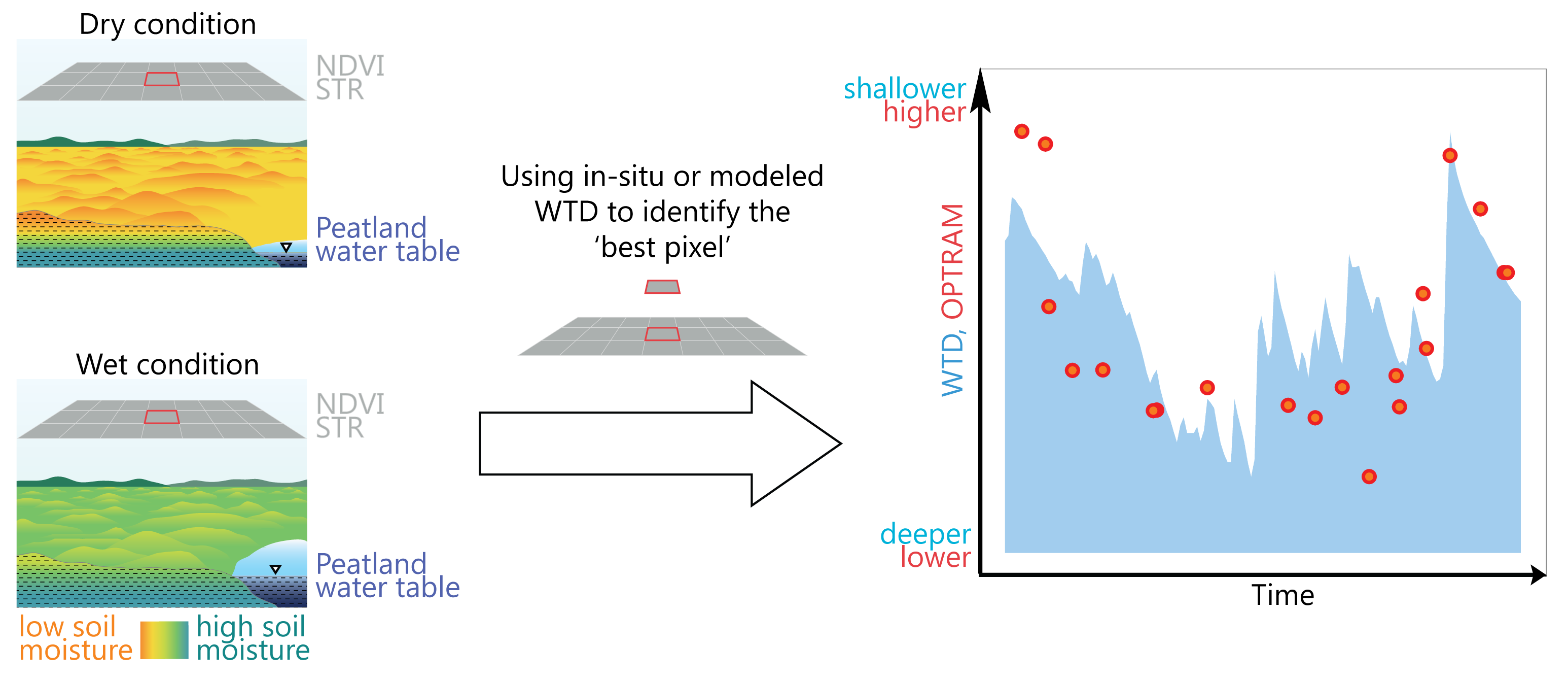
• compare the performance of applying in situ and PEATCLSM WTD data for selecting the ‘best pixels’, i.e., OPTRAM pixels with the highest sensitivity to the in situ WTD fluctuations in peatlands;
• assess the quality of ‘best pixels’ selected based on in situ WTD in comparison to PEATCLSM WTD data for WTD monitoring.

2. Materials and Methods

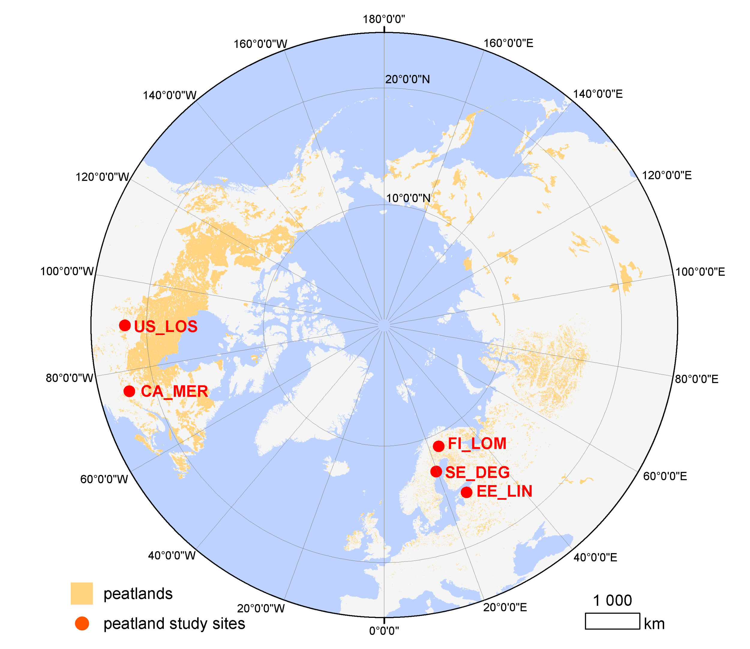
2.1. Study Sites and In Situ WTD Measurements

We used a subset of WTD data from Bechtold et al. [42], which represents a comprehensive data compilation of in situ measurements in northern peatland complexes. Specifically, we selected peatlands with more than 10 years of in situ WTD data to ensure that the study sites were covered by a sufficient number of remote sensing images. In total, data from five peatlands were used in this research (Figure 2). The peatlands included two bogs and three fens (

Table 1. Overview of peatland sites.

Site Name and Location	Site Code	WTD Data Period	Peatland Type	Dominant Vegetation	Lat.	Lon.	Ref.
Linnusaare, Estonia	EE_LIN	2008–2017	bog	Mosses, sedges, shrubs, sparse dwarf pines	58.88	26.20	[46]
Mer Bleue, Canada	CA_MER	2000–2017	bog	Shrubs, sedges, black spruce, mosses	45.41	−75.52	[34,47]
Degerö Stormyr, Sweden	SE_DEG	2002–2017	fen	Sedges, mosses, shrubs	64.18	19.55	[48]
Lompolo-jänkkä, Finland	FI_LOM	2006–2017	fen	Sedges, low shrubs, mosses, downy willows, and dwarf birch	67.99	24.20	[49,50,51]
Lost Creek, USA	US_LOS	2000–2017	fen	Alder, willow, sedges	46.08	−89.97	[52]

).

Table 1 presents an overview of the peatlands. In each peatland, in situ WTD data from one representative monitoring well were used. All the peatlands were characterized by a peat layer of at least 30 cm thickness, a natural or semi-natural state of the peat layer, and shallow WTD that fluctuated most of the time within the top 50 cm of the peat layer and only occasionally dropped deeper [42].

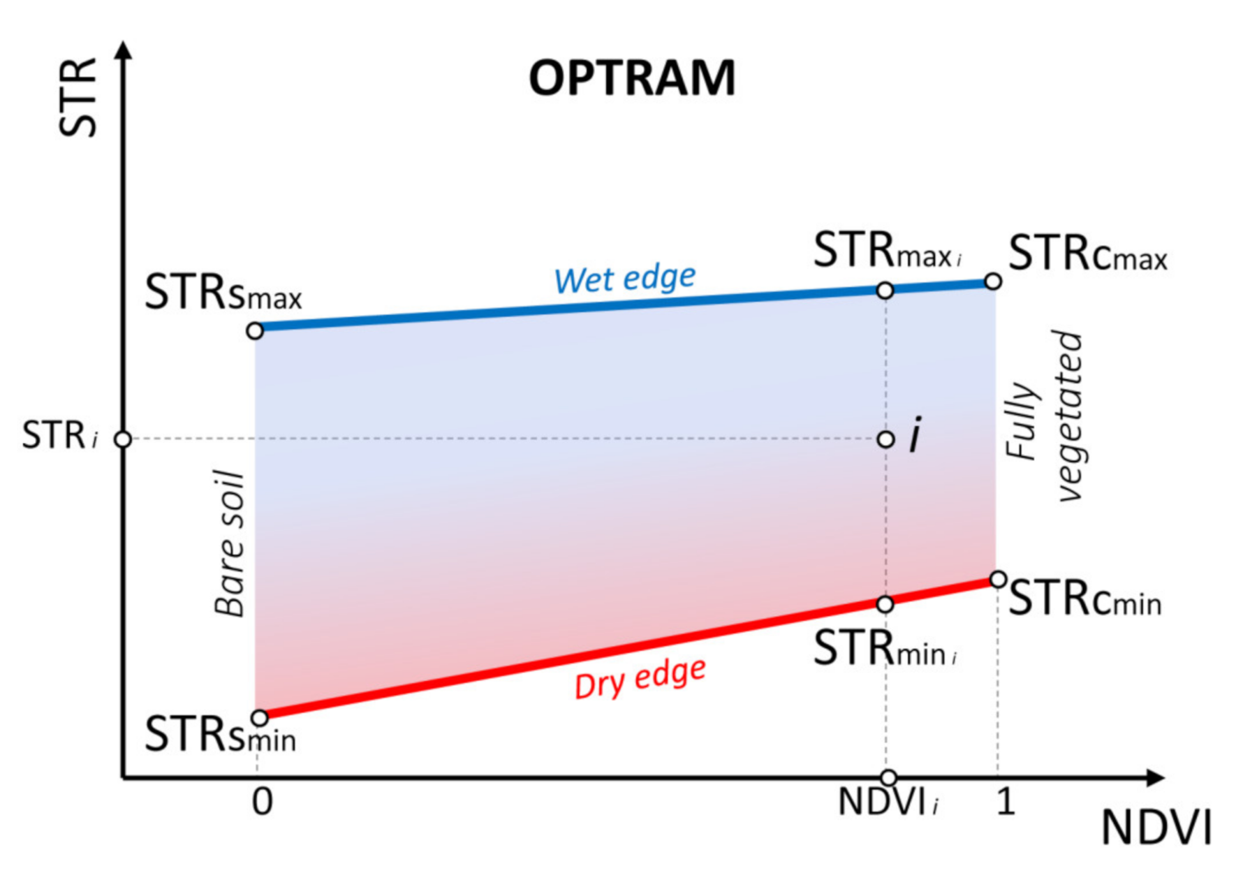
2.2. The OPtical TRApezoid Model (OPTRAM)

2.2.1. Theoretical Background

OPTRAM is a physically-based model proposed by Sadeghi et al. [26]. In comparison to the conventional trapezoid model, where land surface temperature is used instead of STR, OPTRAM utilizes optical data solely. OPTRAM is based on the assumption that the pixels’ distribution within the STR–NDVI space is associated with their moisture availability. Pixels with the highest STR values along the NDVI gradient represent the so-called ‘wet edge’ and they are assumed to have the wettest conditions (Figure 3). Conversely, the pixels with the lowest STR values along the NDVI gradient represent the ‘dry edge’ and they have the lowest moisture availability. In trapezoid models, wet and dry edges are isopleths of uniform soil moisture conditions in different vegetation covers [53].

There are two main assumptions for the approach used in OPTRAM. It requires, firstly, the presence of a linear relationship between surface moisture and SWIR reflectance [54], and secondly, the linear relationship between soil- and vegetation-water content [26]. If these assumptions are fulfilled, the soil moisture content at a given pixel i is estimated as follows:

$$W_{OPTRAM,i}=\frac{ST{R}_i-ST{R}_{min,i}}{ST{R}_{max,i}-ST{R}_{min,i}}$$

(1)

where W_OPTRAM,i is the soil moisture content of the pixel normalized by the local maximum wet soil content, STR_i is the STR value of i pixel, STR_max,i and STR_min,i are the STR values of the dry and wet edges at the NDVI of pixel i. W_OPTRAM,i values vary between 1 for pixels lying on the wet edge, and 0 for pixels lying on the dry edge. The NDVI and STR values of pixels are derived as:

$$NDVI=\frac{{\rho }_{NIR}-{\rho }_{Red}}{{\rho }_{NIR}+{\rho }_{Red}}$$

(2)

$$STR=\frac{{\left(1-{\rho }_{SWIR}\right)}^2}{2{\rho }_{SWIR}}$$

(3)

where ρ_NIR, ρ_Red, and ρ_SWIR are surface reflectance in the near-infrared, red, and SWIR wavebands, respectively. The surface reflectance used for NDVI and STR calculation is a function of the surface properties only and does not depend on the ambient atmospheric parameters. Therefore, the universal parametrization of OPTRAM is feasible for long time-series data [22,24].

2.2.2. OPTRAM Parameterization

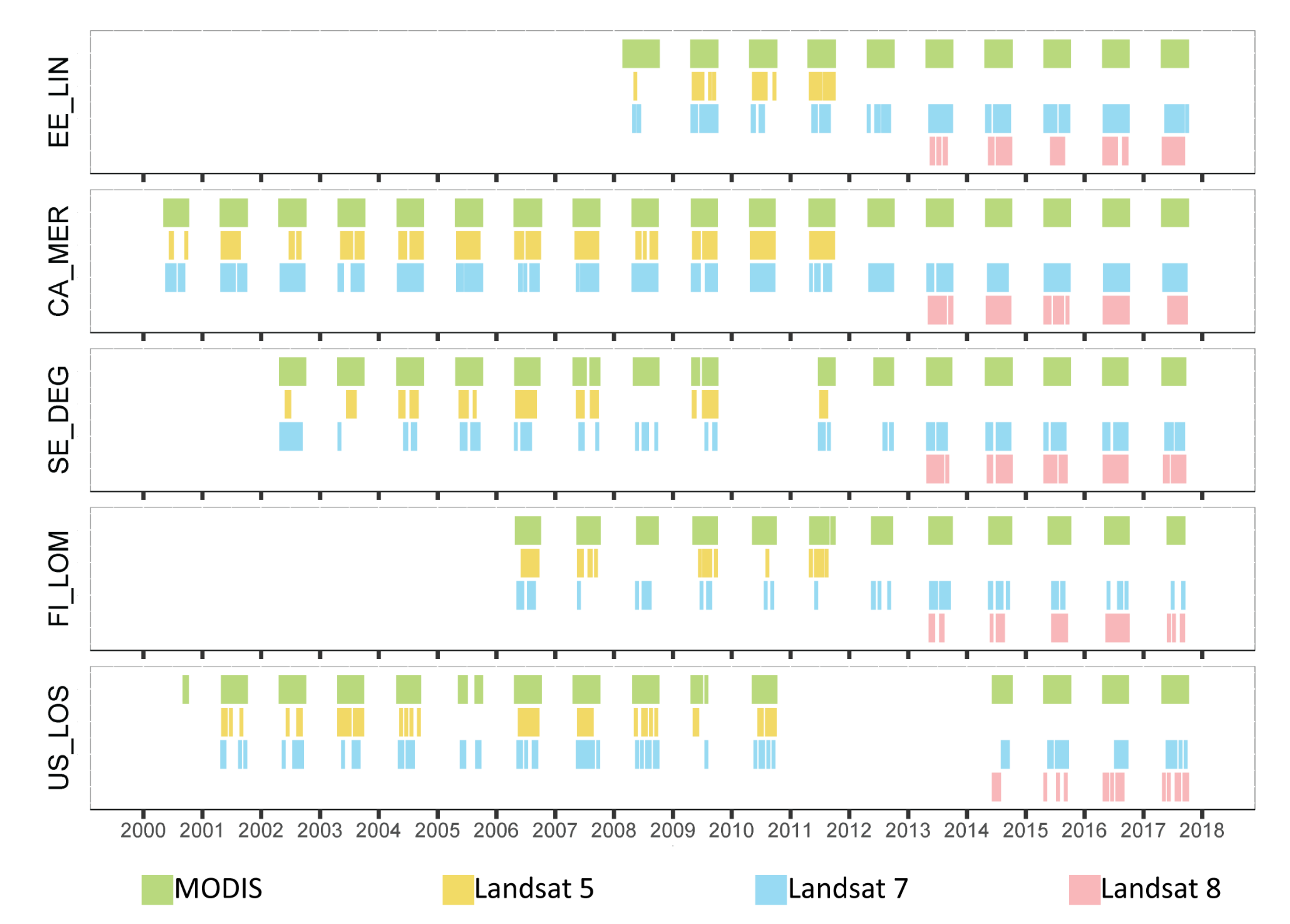
Wet and dry edges are the main isopleths, which delineate the trapezoid space. Different approaches exist to estimate the edges. In most studies, dry and wet edges were subjectively defined based on the visual inspection of NDVI–STR scatterplots [22,24,25,55,56,57]. Babaeian et al. [24] performed a sensitivity analysis of subjectively defined edges and concluded that OPTRAM outputs are not highly sensitive to the edges parametrization. Burdun et al. [27] proposed to estimate the dry edge as a linear fit to the ‘median + standard deviation’ values of 100 NDVI intervals. For some of the peatlands, we observed inadequate determination of wet edges with this approach. Therefore, here we determined the wet and dry edges subjectively using the visual inspection of NDVI–STR scatterplots for each peatland separately.

Since OPTRAM is sensitive to oversaturated pixels [22,26], we excluded pixels with negative NDVI values, which correspond to water surfaces. However, using the NDVI approach, it was not possible to exclude all the pixels with at least some portion of open water since their NDVI values can sometimes be positive. Further, we excluded oversaturated pixels lying above the wet edge and did not use their OPTRAM values in statistical analysis.

2.3. Satellite Data

The OPTRAM index was estimated using Landsat, MODIS, and Landsat spatially aggregated to the MODIS resolution for the years covering in situ WTD measurements. To exclude periods when the peat soil was frozen, the OPTRAM index was calculated for the period from the beginning of May to the end of September. Additionally, we filtered out images for days, when no in situ and modeled WTD data were available. Data processing was performed on the Google Earth Engine (GEE) online platform [58]. All the remotely sensed data were re-projected to WGS 84/Pseudo-Mercator projection (EPSG:3857).

We processed Landsat 5, 7, and 8 surface reflectance data with a 30 m spatial resolution. The Landsat surface reflectance product is available in GEE platform. Areas covered with clouds and shadows were masked using CFMASK information which is included in the Landsat surface reflectance dataset in GEE. SWIR data of band 7 (2.08–2.35 μm in Landsat 5 and 7, and 2.107–2.294 μm in Landsat 8) were used for STR calculation. The spectral difference of these SWIR bands is a source of the potential bias for STR calculation, which was beyond the scope of our methodological framework. To compare the performance of OPTRAM of various spatial resolutions, we also estimated OPTRAM based on MODIS data. MODIS aboard Terra provided MOD09GA daily product with a 500 m spatial resolution. The surface reflectance for band 7 (2.105–2.155 μm) was used for the STR calculation. It is noticeable that Landsat and MODIS data have different ranges of SWIR bands used for the STR calculation. To eliminate the effect of different spectral resolutions, we further upscaled the 30-m Landsat data (further called Landsat_30m) to the 500-m MODIS resolution (Landsat_500m), thereby allowing an assessment of the OPTRAM for various spatial resolutions, while using the same spectral information. The new values of Landsat_500m pixels were estimated as the mean value of the Landsat_30m pixels using the function “reduceResolution()” in GEE. It should be noted that the calculation of mean has the inherent bias of dependency on the extreme values. A comparison of upscaling approaches was, however, beyond the scope of our study. The final number of Landsat and MODIS images correspondingly is the following: 156 and 764 for EE_LIN, 383 and 1316 for CA_MER, 212 and 957 for SE_DEG, 117 and 495 for FI_LOM, and 133 and 897 for US_LOS (Figure 4). A detailed description of the number of images by sensors is given in Table S1.

2.4. PEATCLSM Data

We used a simulation output of PEATCLSM described in Bechtold et al. [42,59] that included the time series of modeled WTD at a 3-h temporal resolution for the five peatlands studied here. PEATCLSM simulations were performed only at the location of the monitoring wells at a 30’’ spatial resolution. We assumed the simulation output of the single grid cell in each of the five peatlands to be representative for the whole peatland as also done for the in situ WTD. It has to be noted that the WTD output of PEATCLSM was based on global forcing data of coarse spatial resolution and on peat hydraulic properties that were spatially uniform for all northern peatlands [42,59]. Thus, even if available, the output at multiple 30’’ grid cells would only show minor spatial variability at the scale of a few kilometers in one peatland. The simulation dataset contains data from January 1988 through December 2017. PEATCLSM WTD data were used for the same days when in situ WTD and remotely sensed data were available. We extracted PEATCLSM output at the times nearest to the Landsat acquisition times.

2.5. Statistical Analysis

Prior to estimating temporal correlation coefficients, we tested the normality of variables’ distributions with the Kolmogorov-Smirnov test (p-value 0.05). A normal distribution was observed for all the variables except in situ WTD at CA_MER and US_LOS peatlands (p-values were 0.001 and 0.03, respectively). During the pre-test, we calculated both Pearson and Spearman correlation coefficients for those sites and results were consistent. Thus, for simplicity, we only provide Pearson correlation coefficients for all sites, including CA_MER and US_LOS.

For each comparison of OPTRAM indices with WTD, the per-pixel temporal Pearson correlation coefficients (R) and anomaly Pearson correlation coefficients (anomR) were estimated. This was done for OPTRAM indices obtained with Landsat_30m, MODIS, and Landsat_500m, and for WTD either in situ or modeled with PEATCLSM. Anomalies were obtained by removing the multi-year one-month smoothed average from the original values.

We performed a random sampling test to validate the stability of spatial patterns of temporal per-pixel correlation. Two randomly selected subsets, each containing 50% of total data in each peatland, were used to calculate R between OPTRAM and in situ WTD (Figure S1).

For each of the three versions of OPTRAM as well as PEATCLSM WTD, 95% confidence intervals (CIs) of the ‘best pixels’ correlation coefficients were estimated, first, for each site, taking into account the reduction of the sample size due to temporal autocorrelation (as in [42,60]). We then aggregated the CIs of the five sites, again separately for each of the three versions of OPTRAM as well as PEATCLSM WTD, by dividing the average of the CIs by the square root of the number of sites [42,60].

2.6. Selection of the OPTRAM Pixel with the Highest R (‘Best Pixel’)

In order to illustrate the difference in the performance of remotely sensed data of various spatial resolutions for monitoring in situ WTD, we compared the highest statistically significant (p-value < 0.05) R value between the OPTRAM index obtained with the various remote sensing data and WTD data (either in situ or modeled). In our study, we focused on the selection of the pixel with the highest R between original (not anomaly) time series of in situ WTD and the OPTRAM index. A selection based on anomR is possible and perhaps even recommendable in preparation for the use of the OPTRAM index in a data assimilation scheme such as the Ensemble Kalman filter [61]. However, due to the relatively limited amount of Landsat data (average of n = 200 per site), the climatology and subsequent anomaly calculation result in anomR values (and spatial patterns) that are noisier than R values. Therefore, we decided to not select the ‘best pixel’ based on anomR, but only to calculate anomR at the location of the pixel with the highest R.

We selected only one ‘best pixel’ per peatland to monitor the temporal dynamics of WTD. Such a study design stemmed from the high sensitivity of OPTRAM to the vegetation cover. This sensitivity limits the spatial interpretability of OPTRAM because of the unknown spatial variability of the soil moisture–WTD relationship. The dates for which OPTRAM information of the ‘best pixels’ was used are presented in Table S2.

3. Results

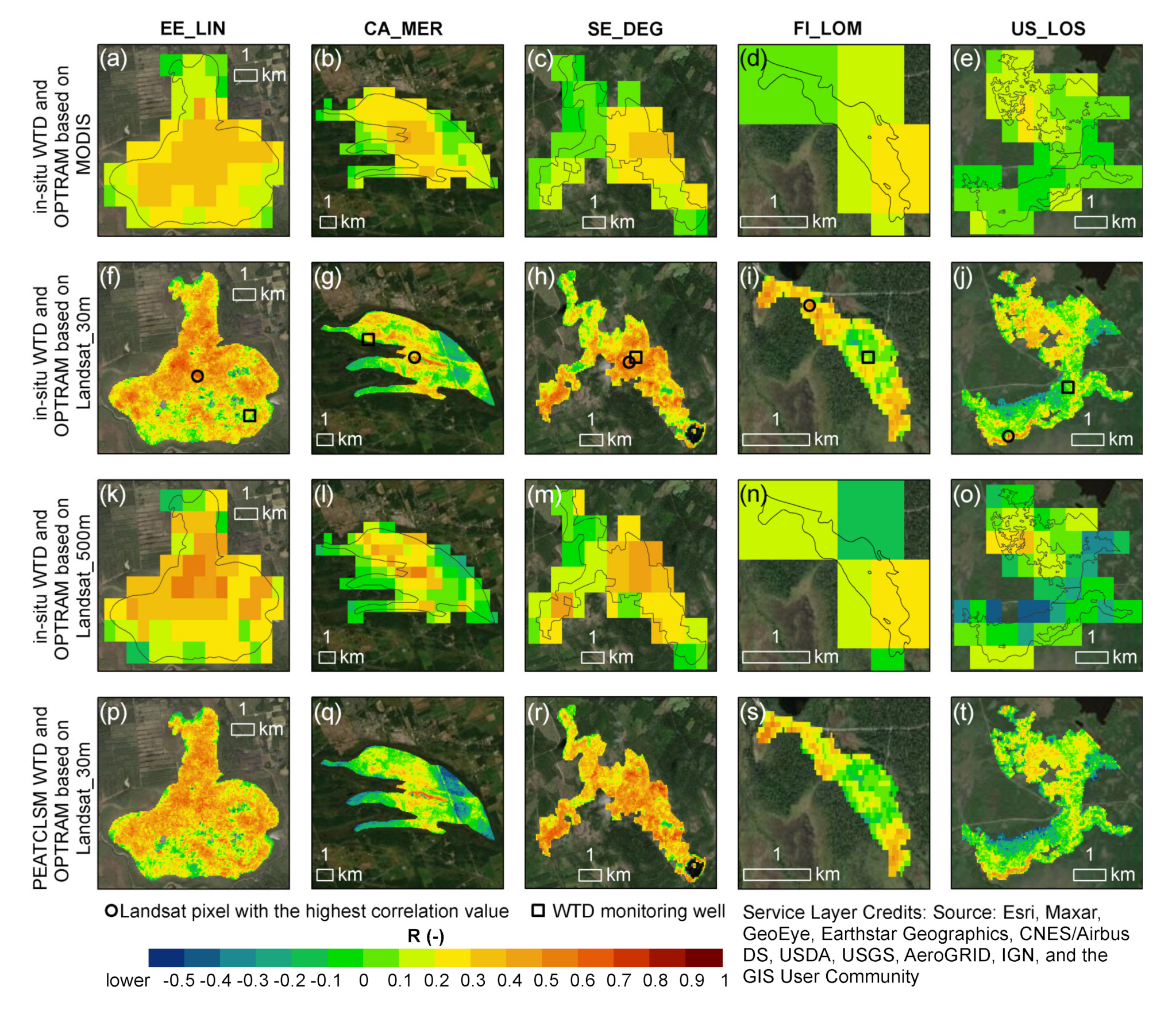
3.1. Spatial Patterns of Temporal Correlation between OPTRAM and WTD

The first objective was to evaluate the applicability of OPTRAM based on remotely sensed data of various spatial resolutions for monitoring temporal changes in WTD measured in situ. Figure 5 shows maps of the per-pixel R values between in situ WTD and OPTRAM based on MODIS (panels a–e), Landsat_30m (panels f–j), and Landsat_500m (panels k–o) data. On the one hand, the different remotely sensed data yielded relatively similar spatial R patterns for all sites (Figure 5, panels a–o). These spatial patterns were similar to those obtained using random sampling (Figure S1). On the other hand, the strength of the correlation varied significantly depending on the remote sensing data used for the OPTRAM calculation. OPTRAM based on MODIS resulted in the lowest scores of the maximum R values. Despite the identical spatial resolution between MODIS and Landsat_500m, the latter had higher values of maximum R metrics. However, the highest values of maximum correlation were observed for OPTRAM based on Landsat_30m. Interestingly, for all the sites except for SE_DEG, the highest R values between in situ WTD and OPTRAM based on Landsat_30m (as the one with the best spatial resolution) were not located close to the WTD monitoring wells (Figure 5, panels f–j). This result supports our assumption that WTD varies rather uniformly within a peatland and, thus, suggests searching in a wider radius for a ‘best pixel’.

In Figure 5 (panels p–t), we also present maps of temporal per-pixel R between PEATCLSM WTD and OPTRAM based on Landsat_30m. When comparing the R maps of panels f–j with panels p–t, we observe a remarkable similarity, even though PEATCLSM is a model designed for global application and therefore lacks local processes and calibration [42]. This result provides an important insight into the feasibility of PEATCLSM for localizing the ‘best pixels’ for WTD monitoring with OPTRAM in peatlands for which no in situ data are available.

3.2. Dependency of the Temporal Correlation between OPTRAM and WTD on Vegetation Cover

Our next objective was to analyze the vegetation cover dependency of the temporal correlation between WTD and OPTRAM, i.e., to attribute vegetation covers to the high (>0.5) and low (<0.1) per-pixel correlation. For this objective, we analyzed the available maps of vegetation distribution in the peatlands.

Table 2. Overview of vegetation cover attributed to the high and low correlation between WTD and OPTRAM.

Site Code	Characteristics of Sites with High R	Characteristics of Sites with Low R
EE_LIN	Hollow-ridge complex with permanently flooded depressions. Pixels’ area is mainly covered with hollows [62,63]. The dominant vegetation is Sphagnum species and graminoids [64].	Hummocks covered with dwarf pines, graminoids, and Sphagnum species [65].
CA_MER	A higher density of hollows microtopography with lower plant area index [66]. Vegetation is dominated by Sphagnum species, evergreen shrubs, deciduous shrubs, and sedges [67,68,69].	Relatively dense tree canopy of black spruce and tamarack [47,66]; drained areas east of ditch with gray birch, tamarack, and white pine [70].
SE_DEG	Permanently flooded Sphagnum-dominated hollows, lawns, and flarks [71,72,73].	Forested peatland with pine and spruce [74].
FI_LOM *	A high percentage of Sphagnum cover (70–98%). Sites are covered with mosses, graminoids, shrubs, and trees. This territory matches with the area covered by vegetation community described as cluster 3 [51].	Corresponds to riparian areas of the stream running through the FI_LOM site. It is primarily vegetated by 60-cm-high Salix [51].
US_LOS	Emergent or wet meadows, and lowland shrubs [75].	Forested wetland and shrubs [75].

* Vegetation data available only for the central part of the peatland.

provides an overview of the vegetation cover for areas with high and low R. Mainly areas with very shallow WTD (hollows or lawns) or permanently flooded conditions that are dominantly covered with mosses and graminoids showed the highest sensitivity of OPTRAM to changes in WTD. In contrast, areas dominantly covered with shrubs and trees showed the lowest sensitivities of OPTRAM to changes in WTD.

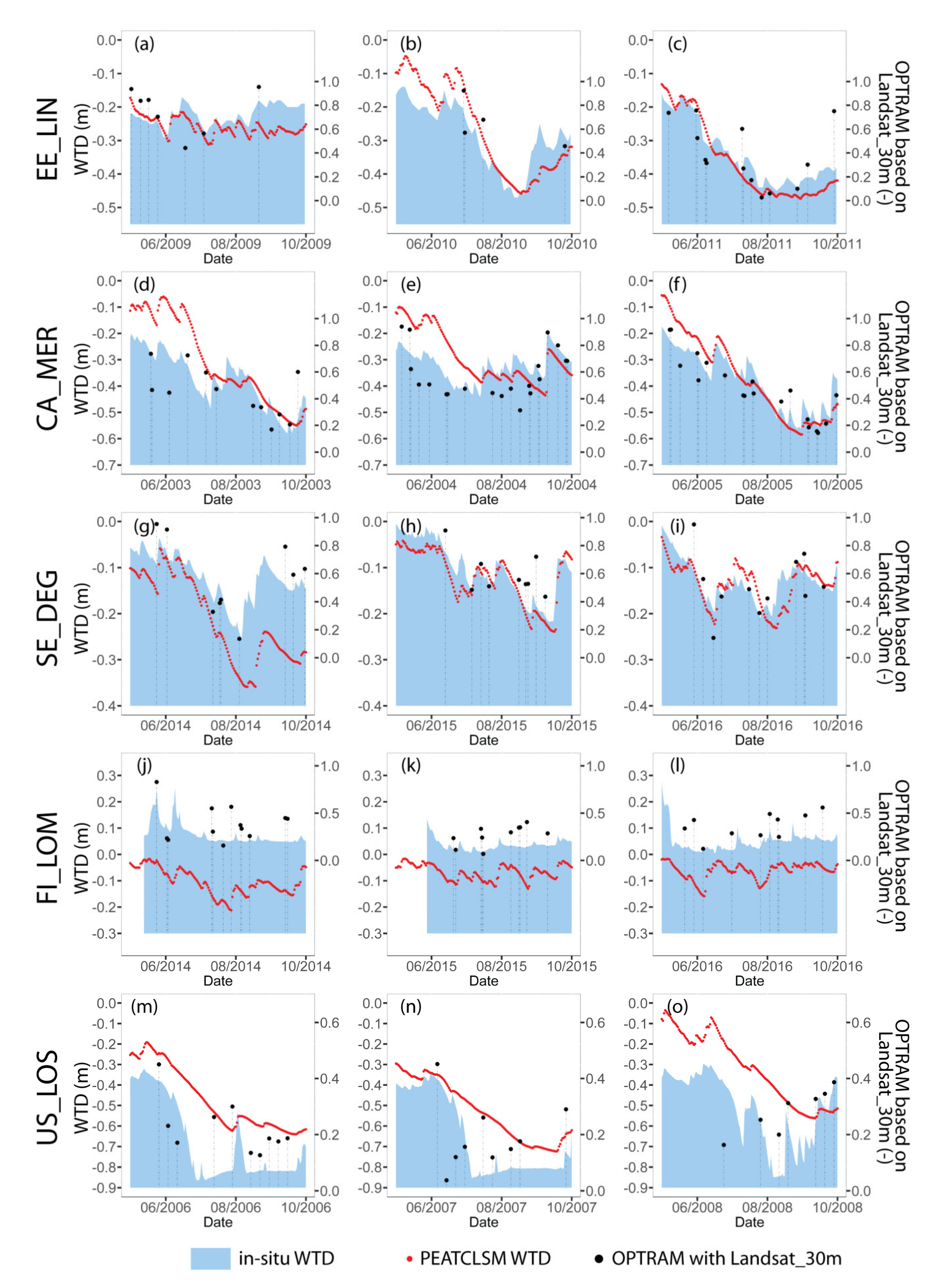
3.3. Temporal Relationships between In Situ WTD and OPTRAM, and between In Situ and Modeled WTD

Another objective of this study was to reveal how well the OPTRAM index or PEATCLSM simulations match in situ observed WTD. As described above, the OPTRAM based on different satellite data resulted in different maximum R values. To highlight this difference, we selected one pixel with the highest R value—the ‘best pixel’—(Figure 5) within each peatland and showed those R together with anomR in Figure 6. The highest mean R between in situ WTD and OPTRAM was observed for OPTRAM based on Landsat_30m, while the lowest R was found for OPTRAM based on MODIS.

Another interesting aspect of Figure 6 is the high temporal R and anomR values between in situ WTD and OPTRAM based on Landsat_30m, which are almost as good as those between in situ WTD and WTD modeled with PEATCLSM. The most remarkable difference between the two can be observed for the FI_LOM site for which OPTRAM based on Landsat_30m performed much better than PEATCLSM. At this site, both the OPTRAM index and PEATCLSM WTD performed worse because peat soil was inundated most of the time.

To show the temporal relationships between WTD and OPTRAM which are reflected with the correlation values in Figure 6, Figure 7 provides scatterplots of OPTRAM based on Landsat_30m vs. in situ WTD and PEATCLSM WTD vs. in situ WTD. OPTRAM based on Landsat_30m and PEATCLSM generally have a similar performance in estimating changes in the in situ WTD: R values ranged from 0.56 to 0.74 (average 0.7) for OPTRAM based on Landsat_30m, and from 0.38 to 0.79 (average 0.65) for PEATCLSM WTD.

To illustrate the consistency in time dynamics between in situ WTD, OPTRAM based on Landsat_30m, and PEATCLSM WTD, the time series of those data for an example period of three consecutive years are given in Figure 8. For better visual comparison, the OPTRAM range was adjusted to the in situ WTD range of each site for the period shown. Generally, OPTRAM estimates exhibit the seasonal cycle of in situ WTD (especially in SE_DEG (panels g–i) and CA_MER (panels d–f) sites) and also short-term dynamics of WTD. However, outliers in the OPTRAM time series are present for each site. The time series of FI_LOM site (panels j–l) clearly show the lowest agreement between OPTRAM and in situ WTD, as well as between PEATCLSM WTD and in situ WTD.

4. Discussion

4.1. Factors Affecting the Ability of OPTRAM Index to Reveal the Changes in WTD

Our study demonstrated that the ability of OPTRAM index in detecting changes in the in situ WTD depends on several factors: (i) The spatial resolution of remotely sensed data used for OPTRAM calculation, and (ii) the dominant vegetation cover within the OPTRAM pixel.

We showed that the OPTRAM index of high spatial resolution (Landsat_30m) had a stronger association with the in situ WTD than OPTRAM of lower spatial resolution (Landsat_500m or MODIS). The poorer performance of Landsat_500m and MODIS could be explained by the high fragmentation of vegetation communities, which appears in hummock-hollow/lawn complexes in peatlands. Data of 500 m spatial resolution seem to be insufficient to capture the SWIR signal over the vegetation cover which showed the highest OPTRAM sensitivity to changes in WTD (Figure 9).

This is the first time that the effect of spatial resolution was revealed to influence OPTRAM performance in peatlands. However, previous research suggests a similar spatial resolution effect on OPTRAM performance in other ecosystems. On average, the association between OPTRAM and soil moisture was shown to be weaker for moderate (R = 0.1–0.7) [24,55] than for high (R = 0.5 and higher) [22,57] and ultrahigh spatial resolutions (R = 0.66–0.83) [26]. However, this comparison should be interpreted with caution because of the differences in the bandwidth of the data used for OPTRAM estimation in those studies. In future work, applying blending techniques, e.g., STARFM [76], could shed more light on spatial scaling effects on OPTRAM accuracy for WTD monitoring.

As we have demonstrated, OPTRAM performances differ for data with a similar spatial resolution (Figure 5). A possible explanation for this might be that Landsat (2.08–2.35 μm in Landsat 5 and 7, and 2.107–2.294 μm in Landsat 8) and MODIS (2.105–2.155 μm) data have different ranges and widths of SWIR bands used for STR calculation. Landsat data with longer SWIR wavelengths and wider SWIR bands resulted in a higher maximum temporal correlation with in situ WTD than the MODIS data with a narrower SWIR band at shorter wavelengths. This result is in line with the study by Sadeghi et al. [54], who illustrated the better performance of longer SWIR wavelengths for soil moisture estimation. This finding suggests that OPTRAM based on Sentinel-2 data (SWIR 2.10–2.28 μm) has a high potential to be used in the future research of WTD monitoring in peatlands. Previous researches indicated that data of narrow SWIR band (wavelengths 2.3 μm) from hyperspectral imagery are highly sensitive to the vegetation conditions in different ecosystems, including wetlands [77,78]. Additional studies may show the potential of OPTRAM based on hyperspectral imagery to reveal the WTD dynamic.

Another possible explanation for a different performance of OPTRAM based on MODIS and Landsat_500m is the different temporal frequency of remotely sensed data. There are many more MODIS observations than Landsat_500m ones (Table S2); thus, these results, therefore, need to be interpreted with caution.

In the current study, OPTRAM temporal correlation metrics were similar among most of the peatlands despite differences in peatland type (bog and fen) and vegetation types (Figure 6). The only exception was the FI_LOM site with the lower temporal correlation between OPTRAM and in situ WTD. In our dataset, FI_LOM was the only peatland with a very high (often above the surface) and stable WTD. It seems possible that for permanently saturated peat soil, vegetation has a less noticeable reaction to changes in soil moisture and WTD. Harris et al. [28] have demonstrated this effect on Sphagnum species, which have an uneven curve of the relationship between remotely based moisture stress index (utilizes SWIR and near-infrared spectra) and volumetric moisture content in the soil. It was surprising that for other sites—with less stable WTD—similar areas with shallow WTD or permanently flooded conditions, dominantly covered with mosses and graminoids had the highest sensitivity of OPTRAM to the changes in WTD.

4.2. Potential of Using In Situ and PEATCLSM WTD for Selecting the OPTRAM Pixels with the Highest Sensitivity to WTD Fluctuations

An additional study objective was to compare the performance of applying in situ and modeled WTD data for selecting the ‘best pixel’ with the highest sensitivity of OPTRAM to WTD fluctuations in peatlands. The results presented in Figure 5 indicate that both in situ and modeled WTD data can be used to localize the pixels for which OPTRAM is most sensitive to temporal changes of WTD. The patterns of high and low correlation coefficients shown in panels f–j of Figure 5 are consistent with those shown in panels p–t. Moreover, with a two-fold random sampling (Figure S1), we have demonstrated that the patterns of high and low correlation values are not random but rather attributed to vegetation cover characteristics within the peatlands. This finding reveals the similar character of modeled WTD and WTD measured in situ, allowing them to be used interchangeably to detect the ‘best pixels’. A concrete application would be to find the ‘best pixel’ based on historical simulations or in situ data and subsequently use OPTRAM data at this pixel to monitor WTD near real-time.

Although our results indicated a high potential of localizing ‘best pixels’ for OPTRAM by using PEATCLSM WTD, there is the risk of a selection bias toward zones in a peatland that is conformed to model physics used in PEATCLSM. The coherence of the WTD fluctuations in peatland is not perfect, and, e.g., variable input fluxes of minerotrophic water, which are not simulated in PEATCLSM, generate some spatial variation of WTD dynamics. Similarly, a selection of the ‘best pixel’ based on only a single in situ location will always be biased toward the WTD dynamics of that specific location. These two limitations are important to keep in mind when using monitoring data based on the ‘best pixel’ approach.

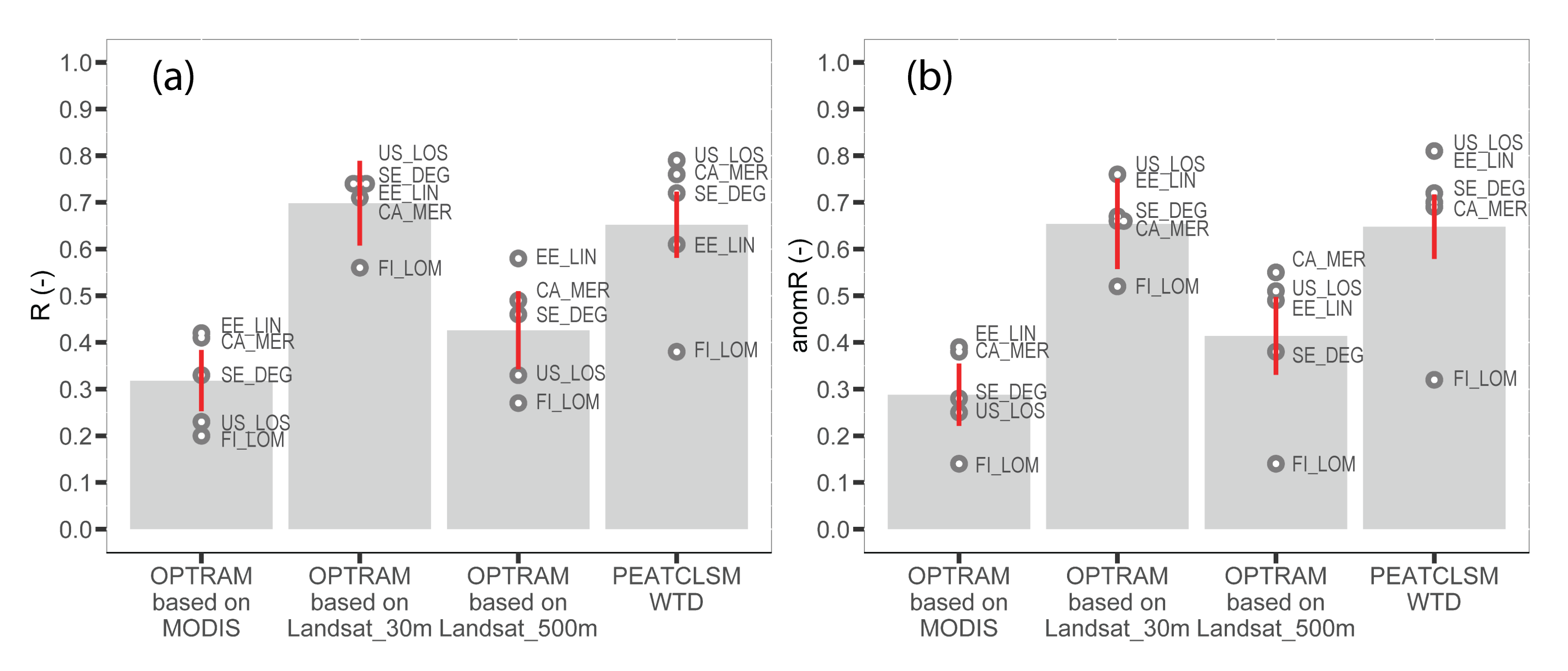
4.3. Quality Assessment of OPTRAM Index in Comparison to PEATCLSM

It was shown that PEATCLSM WTD and OPTRAM based on Landsat_30m demonstrated a similar agreement with in situ WTD (Figure 6). It is interesting to note that for EE_LIN, FI_LOM, and SE_DEG sites OPTRAM performed slightly better than PEATCLSM WTD. Nonetheless, the close inspection of time-series in Figure 8 shows that even for the mentioned sites, some OPTRAM values seem to be outliers and do not correspond to the changes in the in situ WTD, similar outliers were also observed in previous works [27]. The better performance of OPTRAM at some sites could be explained by the fact that PEATCLSM WTD is not always capable of reflecting all fluctuations of in situ WTD [42] either due to the coarse resolution global forcing data or lack of local peatland processes such as the variable dependency of fens to minerotrophic water inputs. Nevertheless, PEATCLSM yielded reasonable spatial patterns of temporal correlation with OPTRAM indices.

Though these results are limited to the small number of peatlands used in this study, the high temporal correlation statistics together with a feasible application for long-term monitoring suggest that the OPTRAM index could be suitable for assimilation into the peatland-specific hydrological models. The OPTRAM index has the potential to contribute independent information to PEATCLSM by providing valuable moisture information at a high spatial resolution. This could potentially correct the errors in PEATCLSM simulations, for example, due to global forcing data of coarse spatial resolution. For example, Bechtold et al. [42] showed a discrepancy between in situ and modeled WTD caused by some (likely local) precipitation events that were not well represented in the global forcing data at approximately 50 km spatial resolution. In the future, such errors could be corrected by assimilating OPTRAM-based moisture observations into PEATCLSM. Moreover, the assimilation of OPTRAM index could add information about temporal WTD dynamics due to anthropogenic disturbance of the hydrological regime in peatlands, a process that is currently not accounted for in PEATCLSM. For this, long-term Landsat observations (>38 years) have a great potential to be used for revealing decade-long moisture changes in peatlands driven not only by climate change but also other more local anthropogenic disturbances.

Despite the promising results, the need to visually determine dry and wet edges using scatterplots of NDVI–STR data for the parameterization of OPTRAM currently limits the global application of OPTRAM and its assimilation into PEATCLSM. Further research should be undertaken to find a robust automatic approach for the determination of dry and wet edges. To date, there is one attempt to estimate OPTRAM in GEE using the automatic parametrization [79]. However, future work is needed to demonstrate the reliability of this approach.

5. Conclusions

This study addressed some challenges of the OPTRAM application in peatlands by using in situ and modeled PEATCLSM WTD data to localize the ‘best pixel’ for monitoring temporal fluctuations of WTD with OPTRAM.

The results of this study indicate that:

• OPTRAM is applicable for monitoring WTD dynamics in both bogs and fen peatland types;
• the spatial resolution of remotely sensed data can impact the quality of OPTRAM index, with better results obtained for high spatial resolution Landsat_30m data;
• the highest temporal correlation coefficients (R = 0.56–0.74, an average of 0.7) between in situ WTD and OPTRAM based on Landsat_30m were observed for pixels with dominantly hollow and lawn microtopography covered with mosses and graminoids with little or no shrubs or trees; and
• either historical in situ WTD or PEATCLSM WTD can be used to detect ‘best’ OPTRAM pixels allowing for subsequent near real-time WTD monitoring using OPTRAM.

Further research should be carried out to explain and minimize outliers of the OPTRAM index and to develop a robust automatized parameterization of OPTRAM over peatlands, which are two important issues for future OPTRAM applications on a global scale. Furthermore, the use of Sentinel-2 data can be recommended to compute the OPTRAM index with an increased temporal resolution. Finally, the high temporal (anomaly) correlation statistics of OPTRAM suggest that there is potential for the assimilation of OPTRAM index into a peatland-specific hydrological model such as PEATCLSM.

References

1. Roulet, N.T.; Lafleur, P.M.; Richard, P.J.H.; Moore, T.R.; Humphreys, E.R.; Bubier, J. Contemporary carbon balance and late Holocene carbon accumulation in a northern peatland. Glob. Chang. Biol. 2007, 13, 397–411. [Google Scholar] [CrossRef] [Green Version]
2. Yu, Z.; Loisel, J.; Brosseau, D.P.; Beilman, D.W.; Hunt, S.J. Global peatland dynamics since the Last Glacial Maximum. Geophys. Res. Lett. 2010, 37. [Google Scholar] [CrossRef]
3. Damman, A.W.H. Peat accumulation in fens and bogs: Effects of hydrology and fertility. In Proceedings of the Northern Peatlands in Global Climatic Change; Publications of the Academy of Finland: Helsinki, Finland, 1996; pp. 213–222. [Google Scholar]
4. Yu, Z.; Beilman, D.W.; Frolking, S.; MacDonald, G.M.; Roulet, N.T.; Camill, P.; Charman, D.J. Peatlands and Their Role in the Global Carbon Cycle. EOS Trans. Am. Geophys. Union 2011, 92, 97–98. [Google Scholar] [CrossRef]
5. Frolking, S.; Roulet, N.T. Holocene radiative forcing impact of northern peatland carbon accumulation and methane emissions. Glob. Chang. Biol. 2007, 13, 1079–1088. [Google Scholar] [CrossRef]
6. Helbig, M.; Waddington, J.M.; Alekseychik, P.; Amiro, B.D.; Aurela, M.; Barr, A.G.; Black, T.A.; Blanken, P.D.; Carey, S.K.; Chen, J.; et al. Increasing contribution of peatlands to boreal evapotranspiration in a warming climate. Nat. Clim. Chang. 2020, 10, 555–560. [Google Scholar] [CrossRef]
7. Hilbert, D.W.; Roulet, N.; Moore, T. Modelling and analysis of peatlands as dynamical systems. J. Ecol. 2000, 88, 230–242. [Google Scholar] [CrossRef]
8. Sulman, B.N.; Desai, A.R.; Saliendra, N.Z.; Lafleur, P.M.; Flanagan, L.B.; Sonnentag, O.; Mackay, D.S.; Barr, A.G.; van der Kamp, G. CO 2 fluxes at northern fens and bogs have opposite responses to inter-annual fluctuations in water table. Geophys. Res. Lett. 2010, 37. [Google Scholar] [CrossRef]
9. Lafleur, P.M.; Moore, T.R.; Roulet, N.T.; Frolking, S. Ecosystem Respiration in a Cool Temperate Bog Depends on Peat Temperature But Not Water Table. Ecosystems 2005, 8, 619–629. [Google Scholar] [CrossRef]
10. Lindholm, T.; Markkula, I. Moisture conditions in hummocks and hollows in virgin and drained sites on the raised bog Laaviosuo, southern Finland. Ann. Bot. Fenn. 1984, 21, 241–255. [Google Scholar] [CrossRef]
11. Kellner, E.; Halldin, S. Water budget and surface-layer water storage in a Sphagnum bog in central Sweden. Hydrol. Process. 2002, 16, 87–103. [Google Scholar] [CrossRef]
12. Price, J.S.; Schlotzhauer, S.M. Importance of shrinkage and compression in determining water storage changes in peat: The case of a mined peatland. Hydrol. Process. 1999, 13, 2591–2601. [Google Scholar] [CrossRef] [Green Version]
13. Entekhabi, D.; Njoku, E.G.; O’Neill, P.E.; Kellogg, K.H.; Crow, W.T.; Edelstein, W.N.; Entin, J.K.; Goodman, S.D.; Jackson, T.J.; Johnson, J.; et al. The soil moisture active passive (SMAP) mission. Proc. IEEE 2010, 98, 704–716. [Google Scholar] [CrossRef]
14. Kerr, Y.H.; Waldteufel, P.; Wigneron, J.P.; Delwart, S.; Cabot, F.; Boutin, J.; Escorihuela, M.J.; Font, J.; Reul, N.; Gruhier, C.; et al. The SMOS Mission: New tool for monitoring key elements of the global water cycle. Proc. IEEE 2010, 98, 666–687. [Google Scholar] [CrossRef] [Green Version]
15. Torres, R.; Snoeij, P.; Geudtner, D.; Bibby, D.; Davidson, M.; Attema, E.; Potin, P.; Rommen, B.Ö.; Floury, N.; Brown, M.; et al. GMES Sentinel-1 mission. Remote Sens. Environ. 2012, 120, 9–24. [Google Scholar] [CrossRef]
16. Mohammadimanesh, F.; Salehi, B.; Mahdianpari, M.; Brisco, B.; Motagh, M. Wetland Water Level Monitoring Using Interferometric Synthetic Aperture Radar (InSAR): A Review. Can. J. Remote Sens. 2018, 44, 247–262. [Google Scholar] [CrossRef]
17. Asmuß, T.; Bechtold, M.; Tiemeyer, B. On the Potential of Sentinel-1 for High Resolution Monitoring of Water Table Dynamics in Grasslands on Organic Soils. Remote Sens. 2019, 11, 1659. [Google Scholar] [CrossRef] [Green Version]
18. Bauer-Marschallinger, B.; Freeman, V.; Cao, S.; Paulik, C.; Schaufler, S.; Stachl, T.; Modanesi, S.; Massari, C.; Ciabatta, L.; Brocca, L.; et al. Toward Global Soil Moisture Monitoring with Sentinel-1: Harnessing Assets and Overcoming Obstacles. IEEE Trans. Geosci. Remote Sens. 2019, 57, 520–539. [Google Scholar] [CrossRef]
19. Tiner, R.W.; Lang, M.W.; Klemas, V. V Remote Sensing of Wetlands: Applications and Advances; CRC Press: Boca Raton, FL, USA, 2015; ISBN 1482237385. [Google Scholar]
20. Bechtold, M.; Schlaffer, S.; Tiemeyer, B.; De Lannoy, G. Inferring Water Table Depth Dynamics from ENVISAT-ASAR C-Band Backscatter over a Range of Peatlands from Deeply-Drained to Natural Conditions. Remote Sens. 2018, 10, 536. [Google Scholar] [CrossRef] [Green Version]
21. Jackson, T.J.; Chen, D.; Cosh, M.; Li, F.; Anderson, M.; Walthall, C.; Doriaswamy, P.; Hunt, E.R. Vegetation water content mapping using Landsat data derived normalized difference water index for corn and soybeans. In Proceedings of the Remote Sensing of Environment; Elsevier: Amsterdam, The Netherlands, 2004; Volume 92, pp. 475–482. [Google Scholar] [CrossRef]
22. Sadeghi, M.; Babaeian, E.; Tuller, M.; Jones, S.B. The optical trapezoid model: A novel approach to remote sensing of soil moisture applied to Sentinel-2 and Landsat-8 observations. Remote Sens. Environ. 2017, 198, 52–68. [Google Scholar] [CrossRef] [Green Version]
23. Goward, S.N.; Cruickshanks, G.D.; Hope, A.S. Observed relation between thermal emission and reflected spectral radiance of a complex vegetated landscape. Remote Sens. Environ. 1985, 18, 137–146. [Google Scholar] [CrossRef]
24. Babaeian, E.; Sadeghi, M.; Franz, T.E.; Jones, S.; Tuller, M. Mapping soil moisture with the OPtical TRApezoid Model (OPTRAM) based on long-term MODIS observations. Remote Sens. Environ. 2018, 211, 425–440. [Google Scholar] [CrossRef]
25. Huang, F.; Wang, P.; Ren, Y.; Liu, R. Estimating Soil Moisture Using the Optical Trapezoid Model (OPTRAM) in a Semi-Arid Area of SONGNEN Plain, China Based on Landsat-8 Data. In Proceedings of the International Geoscience and Remote Sensing Symposium (IGARSS); Institute of Electrical and Electronics Engineers Inc., Yokohama, Japan, 28 July–2 August 2019; pp. 7010–7013. [Google Scholar] [CrossRef]
26. Babaeian, E.; Sidike, P.; Newcomb, M.S.; Maimaitijiang, M.; White, S.A.; Demieville, J.; Ward, R.W.; Sadeghi, M.; LeBauer, D.S.; Jones, S.B.; et al. A New Optical Remote Sensing Technique for High-Resolution Mapping of Soil Moisture. Front. Big Data 2019, 2, 37. [Google Scholar] [CrossRef] [Green Version]
27. Burdun, I.; Bechtold, M.; Sagris, V.; Komisarenko, V.; De Lannoy, G.; Mander, Ü. A comparison of three trapezoid models using optical and thermal satellite imagery for water table depth monitoring in Estonian bogs. Remote Sens. 2020, 12, 1980. [Google Scholar] [CrossRef]
28. Harris, A.; Bryant, R.G.; Baird, A.J. Detecting near-surface moisture stress in Sphagnum spp. Remote Sens. Environ. 2005, 97, 371–381. [Google Scholar] [CrossRef]
29. Bryant, R.G.; Baird, A.J. The spectral behaviour of Sphagnum canopies under varying hydrological conditions. Geophys. Res. Lett. 2003, 30, 1134. [Google Scholar] [CrossRef] [Green Version]
30. Harris, A. Spectral reflectance and photosynthetic properties of Sphagnum mosses exposed to progressive drought. Ecohydrology 2008, 1, 35–42. [Google Scholar] [CrossRef]
31. Rydin, H.; McDonald, A.J.S. Tolerance of Sphagnum to water level. J. Bryol. 1985, 13, 571–578. [Google Scholar] [CrossRef]
32. Murphy, M.T.; Moore, T.R. Linking root production to aboveground plant characteristics and water table in a temperate bog. Plant Soil 2010, 336, 219–231. [Google Scholar] [CrossRef]
33. Strack, M.; Waddington, J.M.; Rochefort, L.; Tuittila, E.S. Response of vegetation and net ecosystem carbon dioxide exchange at different peatland microforms following water table drawdown. J. Geophys. Res. Biogeosciences 2006, 111. [Google Scholar] [CrossRef] [Green Version]
34. Lafleur, P.M.; Hember, R.A.; Admiral, S.W.; Roulet, N.T. Annual and seasonal variability in evapotranspiration and water table at a shrub-covered bog in southern Ontario, Canada. Hydrol. Process. 2005, 19, 3533–3550. [Google Scholar] [CrossRef]
35. Finlayson, C.M.; Milton, G.R. Peatlands. In The Wetland Book II: Distribution, Description, and Conservation; Springer Nature: Berlin/Heidelberg, Germany, 2018; Volume 1, pp. 227–244. ISBN 9789400740013. [Google Scholar]
36. Ivanov, K.E. Water Movement in Mirelands; Academic Press: London, UK, 1981. [Google Scholar]
37. Letts, M.G.; Comer, N.T.; Roulet, N.T.; Skarupa, M.R.; Verseghy, D.L. Parametrization of peatland hydraulic properties for the Canadian land surface scheme. Atmos. Ocean 2000, 38, 141–160. [Google Scholar] [CrossRef]
38. Malhotra, A.; Roulet, N.T.; Wilson, P.; Giroux-Bougard, X.; Harris, L.I. Ecohydrological feedbacks in peatlands: An empirical test of the relationship among vegetation, microtopography and water table. Ecohydrology 2016, 9, 1346–1357. [Google Scholar] [CrossRef]
39. Wilson, P. The Relationship among Micro-Topographic Variation, Water Table Depth and Biogeochemistry in an Ombrotrophic Bog; McGill University: Montreal, QC, Canada, 2012. [Google Scholar]
40. Hokanson, K.J.; Moore, P.A.; Lukenbach, M.C.; Devito, K.J.; Kettridge, N.; Petrone, R.M.; Mendoza, C.A.; Waddington, J.M. A hydrogeological landscape framework to identify peatland wildfire smouldering hot spots. Ecohydrology 2018, 11, e1942. [Google Scholar] [CrossRef] [Green Version]
41. Howie, S.A.; van Meerveld, H.J. Regional and local patterns in depth to water table, hydrochemistry and peat properties of bogs and their laggs in coastal British Columbia. Hydrol. Earth Syst. Sci. 2013, 17, 3421–3435. [Google Scholar] [CrossRef] [Green Version]
42. Bechtold, M.; De Lannoy, G.; Koster, R.D.; Reichle, R.H.; Mahanama, S.; Bleuten, W.; Bourgault, M.A.; Brümmer, C.; Burdun, I.; Desai, A.R.; et al. PEAT-CLSM: A Specific Treatment of Peatland Hydrology in the NASA Catchment Land Surface Model. J. Adv. Model. Earth Syst. 2019, 11, 2130–2162. [Google Scholar] [CrossRef] [Green Version]
43. Koster, R.D.; Suarez, M.J.; Ducharne, A.; Stieglitz, M.; Kumar, P. A catchment-based approach to modeling land surface processes in a general circulation model 1. Model structure. J. Geophys. Res. Atmos. 2000, 105, 24809–24822. [Google Scholar] [CrossRef]
44. Ducharne, A.; Koster, R.D.; Suarez, M.J.; Stieglitz, M.; Kumar, P. A catchment-based approach to modeling land surface processes in a general circulation model 2. Parameter estimation and model demonstration. J. Geophys. Res. Atmos. 2000, 105, 24823–24838. [Google Scholar] [CrossRef]
45. Xu, J.; Morris, P.J.; Liu, J.; Holden, J. PEATMAP: Refining estimates of global peatland distribution based on a meta-analysis. Catena 2018, 160, 134–140. [Google Scholar] [CrossRef] [Green Version]
46. Burdun, I.; Sagris, V.; Mander, Ü. Relationships between field-measured hydrometeorological variables and satellite-based land surface temperature in a hemiboreal raised bog. Int. J. Appl. Earth Obs. Geoinf. 2019, 74, 295–301. [Google Scholar] [CrossRef]
47. Strilesky, S.L.; Humphreys, E.R. A comparison of the net ecosystem exchange of carbon dioxide and evapotranspiration for treed and open portions of a temperate peatland. Agric. For. Meteorol. 2012, 153, 45–53. [Google Scholar] [CrossRef]
48. Peichl, M.; Sagerfors, J.; Lindroth, A.; Buffam, I.; Grelle, A.; Klemedtsson, L.; Laudon, H.; Nilsson, M.B. Energy exchange and water budget partitioning in a boreal minerogenic mire. J. Geophys. Res. Biogeosci. 2013, 118, 1–13. [Google Scholar] [CrossRef]
49. Aurela, M.; Lohila, A.; Tuovinen, J.-P.; Hatakka, J.; Penttilä, T.; Laurila, T. Carbon dioxide and energy flux measurements in four northern-boreal ecosystems at Pallas. Boreal Environ. Res. 2015, 20, 455–473. [Google Scholar]
50. Aurela, M.; Lohila, A.; Tuovinen, J.-P.; Hatakka, J.; Laurila, T.; Riutta, T. Carbon dioxide exchange on a northern boreal fen. J. Name Boreal Environ. Res. 2009, 14, 699–710. [Google Scholar]
51. Räsänen, A.; Aurela, M.; Juutinen, S.; Kumpula, T.; Lohila, A.; Penttilä, T.; Virtanen, T. Detecting northern peatland vegetation patterns at ultra-high spatial resolution. Remote Sens. Ecol. Conserv. 2019, 2, 140. [Google Scholar] [CrossRef] [Green Version]
52. Sulman, B.N.; Desai, A.R.; Cook, B.D.; Saliendra, N.; Mackay, D.S. Contrasting carbon dioxide fluxes between a drying shrub wetland in Northern Wisconsin, USA, and nearby forests. Biogeosciences 2009, 6, 1115–1126. [Google Scholar] [CrossRef] [Green Version]
53. Carlson, T. An Overview of the “Triangle Method” for Estimating Surface Evapotranspiration and Soil Moisture from Satellite Imagery. Sensors 2007, 7, 1612–1629. [Google Scholar] [CrossRef] [Green Version]
54. Sadeghi, M.; Jones, S.B.; Philpot, W.D. A linear physically-based model for remote sensing of soil moisture using short wave infrared bands. Remote Sens. Environ. 2015, 164, 66–76. [Google Scholar] [CrossRef]
55. Chen, M.; Zhang, Y.; Yao, Y.; Lu, J.; Pu, X.; Hu, T.; Wang, P. Evaluation of an OPtical TRApezoid Model (OPTRAM) to retrieve soil moisture in the Sanjiang Plain of Northeast China. Earth Space Sci. 2020, 7. [Google Scholar] [CrossRef]
56. Ambrosone, M.; Matese, A.; Di Gennaro, S.F.; Gioli, B.; Tudoroiu, M.; Genesio, L.; Miglietta, F.; Baronti, S.; Maienza, A.; Ungaro, F.; et al. Retrieving soil moisture in rainfed and irrigated fields using Sentinel-2 observations and a modified OPTRAM approach. Int. J. Appl. Earth Obs. Geoinf. 2020, 89, 102113. [Google Scholar] [CrossRef]
57. Mananze, S.; Pôças, I. Agricultural drought monitoring based on soil moisture derived from the optical trapezoid model in Mozambique. J. Appl. Remote Sens. 2019, 13, 1. [Google Scholar] [CrossRef]
58. Gorelick, N.; Hancher, M.; Dixon, M.; Ilyushchenko, S.; Thau, D.; Moore, R. Google Earth Engine: Planetary-scale geospatial analysis for everyone. Remote Sens. Environ. 2017, 202, 18–27. [Google Scholar] [CrossRef]
59. Bechtold, M.; De Lannoy, G.; Reichle, R.H. PEAT-CLSM Simulation Output (Northern Peatlands) Version 1. Available online: https://osf.io/e58ym/ (accessed on 1 July 2020).
60. De Lannoy, G.J.M.; Reichle, R.H. Global assimilation of multiangle and multipolarization SMOS brightness temperature observations into the GEOS-5 catchment land surface model for soil moisture estimation. J. Hydrometeorol. 2016, 17, 669–691. [Google Scholar] [CrossRef] [Green Version]
61. Bechtold, M.; De Lannoy, G.; Reichle, R.H.; Roose, D.; Balliston, N.; Burdun, I.; Devito, K.; Kurbatova, J.; Munir, T.M.; Zarov, E.A. Improved Groundwater Table and L-band Brightness Temperature Estimates for Northern Hemisphere Peatlands Using New Model Physics and SMOS Observations in a Global Data Assimilation Framework. Remote Sens. Environ. 2020, 246, 111805. [Google Scholar] [CrossRef]
62. Estonian Land Board Download Topographic Data. Available online: https://geoportaal.maaamet.ee/index.php?lang_id=2&page_id=618 (accessed on 21 February 2020).
63. Estonian Land Board Orthophotos. Available online: https://geoportaal.maaamet.ee/index.php?page_id=309&lang_id=2 (accessed on 2 July 2020).
64. Lode, E.; Küttim, M.; Kiivit, I.K. Indicative effects of climate change on groundwater levels in estonian raised bogs over 50 years. Mires Peat 2017, 19. [Google Scholar] [CrossRef]
65. Keskkonnaagentuur. Maastike Kaugseire 2002; Keskkonnaagentuur: Tallinn, Estonia, 2002. [Google Scholar]
66. Arroyo-Mora, J.P.; Kalacska, M.; Soffer, R.J.; Moore, T.R.; Roulet, N.T.; Juutinen, S.; Ifimov, G.; Leblanc, G.; Inamdar, D.; Arroyo-Mora, J.P.; et al. Airborne Hyperspectral Evaluation of Maximum Gross Photosynthesis, Gravimetric Water Content, and CO2 Uptake Efficiency of the Mer Bleue Ombrotrophic Peatland. Remote Sens. 2018, 10, 565. [Google Scholar] [CrossRef] [Green Version]
67. Li, J.; Chen, W.; Touzi, R. Optimum RADARSAT-1 configurations for wetlands discrimination: A case study of the Mer Bleue peat bog. Can. J. Remote Sens. 2007, 33, S46–S55. [Google Scholar] [CrossRef]
68. Sonnentag, O.; Chen, J.M.; Roberts, D.A.; Talbot, J.; Halligan, K.Q.; Govind, A. Mapping tree and shrub leaf area indices in an ombrotrophic peatland through multiple endmember spectral unmixing. Remote Sens. Environ. 2007, 109, 342–360. [Google Scholar] [CrossRef]
69. Kalacska, M.; Arroyo-Mora, J.; de Gea, J.; Snirer, E.; Herzog, C.; Moore, T. Videographic Analysis of Eriophorum Vaginatum Spatial Coverage in an Ombotrophic Bog. Remote Sens. 2013, 5, 6501–6512. [Google Scholar] [CrossRef] [Green Version]
70. Talbot, J.; Richard, P.J.H.; Roulet, N.T.; Booth, R.K. Assessing long-term hydrological and ecological responses to drainage in a raised bog using paleoecology and a hydrosequence. J. Veg. Sci. 2010, 21, 143–156. [Google Scholar] [CrossRef]
71. Arens, M. The Effect of Spatial Organization of Peatland Patterns on the Hydrology. Master’s Thesis, Wageningen University, Wageningen, The Netherlands, 2017. [Google Scholar]
72. Osterwalder, S.; Sommar, J.; Åkerblom, S.; Jocher, G.; Fritsche, J.; Nilsson, M.B.; Bishop, K.; Alewell, C. Comparative study of elemental mercury flux measurement techniques over a Fennoscandian boreal peatland. Atmos. Environ. 2018, 172, 16–25. [Google Scholar] [CrossRef]
73. Nijp, J.J.; Metselaar, K.; Limpens, J.; Bartholomeus, H.M.; Nilsson, M.B.; Berendse, F.; van der Zee, S.E.A.T.M. High-resolution peat volume change in a northern peatland: Spatial variability, main drivers, and impact on ecohydrology. Ecohydrology 2019, 12, e2114. [Google Scholar] [CrossRef] [Green Version]
74. ICOS Degerö Vegetation. Available online: https://www.icos-sweden.se/station_degero.html (accessed on 1 July 2020).
75. Wiscland 2 Land Cover Database. Available online: https://dnr.wisconsin.gov/maps/WISCLAND.html (accessed on 26 June 2020).
76. Gao, F.; Masek, J.; Schwaller, M.; Hall, F. On the blending of the landsat and MODIS surface reflectance: Predicting daily Landsat surface reflectance. IEEE Trans. Geosci. Remote Sens. 2006, 44, 2207–2218. [Google Scholar] [CrossRef]
77. DuBois, S.; Desai, A.R.; Singh, A.; Serbin, S.P.; Goulden, M.L.; Baldocchi, D.D.; Ma, S.; Oechel, W.C.; Wharton, S.; Kruger, E.L.; et al. Using imaging spectroscopy to detect variation in terrestrial ecosystem productivity across a water-stressed landscape. Ecol. Appl. 2018, 28, 1313–1324. [Google Scholar] [CrossRef] [PubMed]
78. Serbin, S.P.; Singh, A.; Desai, A.R.; Dubois, S.G.; Jablonski, A.D.; Kingdon, C.C.; Kruger, E.L.; Townsend, P.A. Remotely estimating photosynthetic capacity, and its response to temperature, in vegetation canopies using imaging spectroscopy. Remote Sens. Environ. 2015, 167, 78–87. [Google Scholar] [CrossRef]
79. Firigato, J.O. Soil_Moisture_OPTRAM_Sentinel2. Available online: https://github.com/joaootavio007/Google-Earth-Engine/blob/a57546b6da32bb3df2b672cdc1714b71b75954f1/Soil_Moisture_OPTRAM_Sentinel2.js (accessed on 22 August 2020).
Figure 1. Schematic illustration of the approach proposed in this study. The ‘best pixel’ for the monitoring of water table depth (WTD) fluctuations with the OPtical TRApezoid Model (OPTRAM) index can be localized by WTD data either measured or modeled for a single location. The underlying assumption of this approach is that WTD fluctuations are synchronous in a peatland over several kilometers, while the spatial variability is mainly in the long-term mean value of WTD and the amplitude of fluctuations, both not affecting correlation metrics.
Remotesensing 12 02936 g001
Figure 2. Study sites (red dots) and distribution of northern peatlands (based on Xu et al. [45]). The abbreviations of peatlands are given in Table 1.
Remotesensing 12 02936 g002
Figure 3. The concept of OPTRAM to retrieve a soil moisture index at the point i as a function of normalized difference vegetation index (NDVI) and short-wave infrared transformed reflectance (STR). The wet edge is shown with a blue line and indicated by points STRsmax and STRcmax. The dry edge is shown with the red line and indicated by points STRsmin and STRcmin. The color gradient indicates the transition of moisture condition from the wet to dry edges. Point i with STRi and NDVIi represents moderate moisture availability. For i, the STR values of the wet and dry edges are STRmaxi and STRmini correspondingly.
Remotesensing 12 02936 g003
Figure 4. Temporal distribution of remotely sensed MODIS and Landsat images. The abbreviations of peatlands are given in Table 1.
Remotesensing 12 02936 g004
Figure 5. The temporal per-pixel correlation (R) between in situ water table depth (WTD) and OPTRAM based on Landsat_30m (a–e), MODIS (f–j) and Landsat_500m (k–o), and between WTD modeled with PEATCLSM and OPTRAM based on Landsat_30m (p–t). Panels f–j show the location of the monitoring wells (black square) and the pixels of Landsat_30m data with the highest temporal correlation with in situ WTD, i.e., the ‘best pixel’ (black circle). The abbreviations of peatlands are given in Table 1.
Remotesensing 12 02936 g005
Figure 6. Temporal Pearson correlation coefficients between in situ water table depth (WTD) and three versions of OPTRAM as well as PEATCLSM WTD for (a) original (R) and (b) anomaly (anomR) time series data. R and anomR are shown only for pixels with the highest R value within each peatland site, i.e., the ‘best pixel’, and for PEATCLSM WTD and in situ WTD (data taken for the same days as for estimating R between in situ WTD and OPTRAM based on Landsat_30m). The black dots and text on the right-hand side of these dots present the R and anomR values of the selected pixel and site code where this pixel is located. The height of the bars indicates the mean value of R and anomR. The error bars represent the 95% confidence intervals after having taken into account the temporal autocorrelation. The abbreviations of peatlands are given in Table 1.
Remotesensing 12 02936 g006
Figure 7. Scatterplots of (panels a–e) in situ water table depth (WTD) and OPTRAM based on Landsat_30m ‘best pixel’, and (panels f–j) in situ WTD and PEATCLSM WTD taken for the same days as for OPTRAM based on Landsat_30m and in situ WTD. The abbreviations of peatlands are given in Table 1.
Remotesensing 12 02936 g007
Figure 8. Exemplary three-year periods (vegetation season only) of the long-term time series of water table depth (WTD) measured in situ and modeled with PEATCLSM, and OPTRAM based on Landsat_30m for EE_LIN (panels a–c), CA_MER (panels d–f), SE_DEG (panels g–i), FI_LOM (panels j–l) and US_LOS (panels m–o). OPTRAM values are shown for the ‘best pixel’ within each peatland site. For better visual comparison, the OPTRAM range is adjusted to the in situ WTD range of each site for the shown period. The abbreviations of peatlands are given in Table 1.
Remotesensing 12 02936 g008
Figure 9. Comparison of the area represented by one Landsat pixel (a) and one MODIS pixel (b). The location of the Landsat_30m ‘best pixel’ in the EE_LIN site is shown.
Remotesensing 12 02936 g009