New Insights into Long-Term Aseismic Deformation and Regional Strain Rates from GNSS Data Inversion: The Case of the Pollino and Castrovillari Faults

Abstract

We present a novel inverse method for discriminating regional deformation and long-term fault creep by inversion of GNSS velocities observed at the spatial scale of intraplate faults by exploiting the different spatial signatures of these two mechanisms. In doing so our method provides a refined estimate of the upper bound of the strain accumulation process. As case study, we apply this method to a six year GNSS campaign (2003–2008) set up in the southern portion of the Pollino Range over the Castrovillari and Pollino faults. We show that regional deformation alone cannot explain the observed deformation pattern and implies high geodetic strain rate, with a WSW-ENE extension of $86\pm 41\times {10}^{-9}/\mathrm{yr}$. Allowing for the possibility of fault creep, the modelling of GNSS velocities is consistent with their uncertainties and they are mainly explained by a shallow creep over the Pollino fault, with a normal/strike-slip mechanism up to 5 mm/yr. The regional strain rate decrease by about 70 percent and is characterized by WNW-ESE extension of $24\pm 28\times {10}^{-9}/\mathrm{yr}$. The large uncertainties affecting our estimate of regional strain rate do not allow infering whether the tectonic regime of the area is extensional or strike-slip, although the latter is slightly more likely.

1. Introduction

Geodetic strain rates from GNSS observations, once compared with past and ongoing seismicity, provide a first estimate of the amount of deformation that is accommodated by earthquakes [1,2,3]. This comparison, nevertheless, still leaves open the issue of whether the difference between seismic and GNSS deformation is accommodated by aseismic phenomena or by elastic accumulation preparing the next earthquake [4]. In this respect, geodetic strain rates and earthquake catalogs can only provide an upper bound for the building of the elastic stress.

The main seismic and aseismic phenomena occur at the plate boundary and interseismic deformation from GNSS network are usually modelled by the back-slip approach [5,6] and within the framework of elastic or viscoelastic Earth models [7,8]. These models allow estimating the spatial distribution of the interseismic locking of the interplate faults and, therefore, quantify their elastic loading during the seismic cycle. Considering the large spatial scales of the interseismic deformation at plate boundaries, even sparse GNSS networks can provide valuable information, but difficulties arise in discriminating transient and (long-term) inter seismic deformations due to the limited time intervals spanned by the GNSS data time series [7].

Conversely, interseismic deformation within the plates are the results of elastic deformation mainly caused by the relative motion between plates and by inelastic deformations such as brittle fractures and plastic and ductile flows [9]. The treatment of the lithosphere as a viscous fluid is widely adopted in models of long timescale geological processes. In particular, over geological times and regional spatial scales, this complexity can be taken into account by means of an effective viscosity representing the vertical averaged strength of the lithosphere, as in Splendore and Marotta [10]. This effective viscosity is a key parameter within a thin sheet modelling [11], which allows estimating the surface velocities and the geodetic strain rates due to active tectonics and to provide a first understanding of the average intraplate stress e.g., [12,13,14,15]. These insights are appropriate for the modelling of steady-state tectonic deformation and can be hardly translated into the understanding of how strain is accumulated and released at the time scales of the seismic cycle and at the spatial scales of individual faults. Indeed, by definition, viscoelastoplastic Earth models filter out any short-term and small-scale fluctuations of the elastic stress field.

Due to the these difficulties in dealing with intraplate deformations at small time and spatial scales, GNSS observations are usually used to investigate coseismic and postseismic deformations e.g., [16,17] or transient deformations due to temporary changes in the fault creep [18,19], at least when these phenomena yield deformations high enough to be discriminated from long-term trends. In light of this, by fitting linear trends to GNSS data time series, these approaches always avoid the physical modelling of long-term interseismic deformation and, so, they lose the possibility of understanding how much of this deformation is accommodated by long-term tectonics or by steady-state fault creep or, at least, fault-creep lasting more than the time interval spanned by GNSS data. In other words, we are left with the possibility that the whole amount of long-term strain rate inferred from the linear trends at different GNSS stations is building elastic stress and, then, preparing the next earthquakes, when instead some fraction of it could be caused by inelastic processes that we are actually able to model.

To remedy to this lack of the previous approaches and further refine the upper bound for the elastic loading inferred from geodetic strain rates, we develop a novel approach for modelling GNSS velocities that allow estimating long-term creep over intraplate faults by taking advantages of the different spatial signatures of the main physical mechanism responsible for crustal displacements. As case study, we consider the area of the Pollino Range, which represents the most prominent seismic gap within the southern Apennines [20] and, so, likely affected by aseismic processes able to counteract the intraplate elastic loading. In particular, we focus our attention on the southern area of the Pollino Range and part of the Sybari plain. As shown in Figure 1, this area is crossed by two main faults: the Pollino master fault along the southern slope of Mount Pollino massif and the Castrovillari second-order cross fault [21]. While the whole area of the Pollino Range has been affected only by moderate seismicity in the range of magnitude 5.5∼6 in the last centuries [22], its southern portion is characterized by an even lower seismic activity (see Figure 2). Moreover, also the recent 2010–2014 seismic swarm (main shock $M_{\mathrm{W}}5.1$) accompanied by a significant transient creep (equivalent to $M_{\mathrm{W}}5.5$) has affected the Pollino Range a little further north, activating the Rotonda-Campotenese normal fault system and the Morano Calabro-Piano di Ruggio fault [18], but not its most southern area. The distinctive behaviour of this area is also supported by seismic tomography [23] which has identified it as a low P- and S-wave velocity zone, compared to the northern part of the Pollino Range and the further south Mount Sila massif (see Figure 2), and by the correlation between the high seismicity in high P-wave velocity zones and low seismicity in low P- and S-wave velocity zones. Based on the regional pattern of P-wave receiver functions, seismicity and SKS anisotropy, Chiarabba et al. [24] have suggested that these faults decouple the deformation across the region, from the one driven by the delamination of the southern Apennines to the one related to the retreat mechanism in the Calabrian Subduction System fore arc.

Geomorphic and trenching investigations identified at least six surface-faulting earthquakes of magnitude 6.5∼7 since late Pleistocene age on the Castrovillari and Pollino faults, with the most recent on the Pollino fault and dated in between the XIII and XV century A.D., although no evidence has been found in the historical records Figure 2 [20,21]. Therefore both faults proved to be capable of generating earthquakes of magnitude up to the typical maximum magnitude of Calabria and of the southern Apennines, as large as 7. It is thus important to determine whether aseismic processes are playing a role in inhibiting the seismic potential of these faults or rather to increase it.

The possibility of fault creep on the Castrovillari fault has been already proposed by Sabadini et al. [25] on the basis of surface horizontal velocities estimated at 10 sites by a six year campaign GNSS network from 2003 up to 2008 (see Figure 1). Starting from this previous study, we hereinafter make a step ahead in the modelling of GNSS velocities (i) allowing for the possibility of creep even on the nearby Pollino fault, which could have affected the observed surface velocity as well, and (ii) developing a new inverse method able to discriminate the local contribution due to these creeping faults from the regional one due to large scale intraplate deformations. By jointly estimating the fault creep and the regional deformation from GNSS data inversion, we then aim at defining a more realistic upper bound for the elastic deformation of the southern part of the Pollino Range than that directly provided by geodetic strain rates.

2. Forward Model

We assume that the investigated region is elastic but for the possibility of inelastic deformation localized on the Castrovillari and Pollino faults, and decompose the horizontal velocities $\mathbf{v}$ at the Earth surface as follows

$$\mathbf{v}(\varphi ,\theta )=\left(\begin{array}{c}{v}_{\varphi }(\varphi ,\theta )\\ v_{\theta }(\varphi ,\theta )\end{array}\right)={\mathbf{v}}^{\mathrm{reg}}(\varphi ,\theta )+{\mathbf{v}}^{\mathrm{creep}}(\varphi ,\theta )$$

(1)

where $\varphi$ and $\theta$ are the longitude and latitude at the observation point, $v_{\varphi }$ and $v_{\theta }$ are the east and north components of the velocity field, and ${\mathbf{v}}^{\mathrm{reg}}$ and ${\mathbf{v}}^{\mathrm{creep}}$ are the velocities due to regional deformation and fault creep, respectively. For the sake of simplicity, we do not discuss the up component of the velocity because it is not used in the following inversion of the GNSS data by Sabadini et al. [25].

We note that not all the regional deformation must be elastic simply because aseismic processes other than those here considered could contribute to it. In this respect and as already argued in Section 1, the above decomposition shall be regarded as a conservative choice aiming at refining the upper bound for elastic deformation. If aseismic processes other than those on the faults here considered are modelled, this upper bound will be further refined.

2.1. Regional Deformation

Following Savage et al. [30], within the assumption that the regional deformation varies on spatial scales larger than those of the investigated region and that the topography elevation is small compared to the horizontal distances involved, the horizontal velocity due to regional deformation can be expanded in Taylor series at a reference point $({\varphi }_0,{\theta }_0)$ as follows

$${\mathbf{v}}^{\mathrm{reg}}(\varphi ,\theta )=\mathbf{W}(\varphi ,\theta )\mathbf{w}+\mathbf{E}(\varphi ,\theta )\mathbf{e}$$

(2)

where $\mathbf{W}$, $\mathbf{E}$, $\mathbf{w}$ and $\mathbf{e}$ are the following $2\times 3$–dimensional matrices and 3–dimensional arrays

$$\begin{gathered} \mathbf{W}(\varphi ,\theta )=\left(\begin{array}{ccc}1& sin{\theta }_0\mathrm{d}\varphi & -a\mathrm{d}\theta \\ -sin{\theta }_0\mathrm{d}\varphi & 1& acos{\theta }_0\mathrm{d}\varphi \end{array}\right),\mathbf{E}(\varphi ,\theta )=a\left(\begin{array}{ccc}{cos}_0{\theta }_0\mathrm{d}\varphi & 0& \mathrm{d}\theta \\ 0& \mathrm{d}\theta & cos{\theta }_0\mathrm{d}\varphi \end{array}\right), \\ \mathbf{w}=\left(\begin{array}{c}{v}_{\varphi }^{\mathrm{reg}}({\varphi }_0,{\theta }_0)\\ v_{\theta }^{\mathrm{reg}}({\varphi }_0,{\theta }_0)\\ \omega \end{array}\right),\mathbf{e}=\left(\begin{array}{c}{ϵ}_{\varphi \varphi }\\ {ϵ}_{\theta \theta }\\ {ϵ}_{\theta \varphi }\end{array}\right) \end{gathered}$$

(3)

Here a is the Earth radius, ${ϵ}_{\alpha \beta }$ (with $\alpha ,\beta =\varphi ,\theta$) are the horizontal components of the regional strain rate in the geographic reference system, $\omega$ is the regional rotation rate and

$$\mathrm{d}\varphi =\varphi -{\varphi }_0,\mathrm{d}\theta =\theta -{\theta }_0$$

(4)

In light of this, the regional horizontal velocity field depends on six unknowns, $\mathbf{w}$ and $\mathbf{e}$. We note that the parameters $\mathbf{w}$ describe the rigid-body motion and are equivalent to the three rotation parameters defining the Euler vector [30,31].

In view of the assumptions of elastic body and traction free at Earth surface used to obtain Equation (2), we note also that the vertical components of the regional strain rates read

$${ϵ}_{r\varphi }=0,{ϵ}_{r\theta }=0,{ϵ}_{rr}=-\frac{\lambda }{\lambda +2\mu }\left({ϵ}_{\varphi \varphi }+{ϵ}_{\theta \theta }\right)$$

(5)

with $\mu$ and $\lambda$ being the two Lamé parameters. In the perspective of linking the regional strain rates to the tectonic regimes, it is convenient to express them in terms of the deviatoric components

$${ϵ}_{\alpha \beta }^{\prime }={ϵ}_{\alpha \beta }-\frac{1}{3}{\delta }_{\alpha \beta }\left({ϵ}_{\varphi \varphi }+{ϵ}_{\theta \theta }+{ϵ}_{rr}\right)\forall \alpha ,\beta =\varphi ,\theta ,r$$

(6)

with ${\delta }_{\alpha \beta }$ being the Kronecker delta. After some straightforward algebra, we write

$$\mathbf{e}=\mathbf{D}\mathbf{q}$$

(7)

where

$$\mathbf{D}=\left(\begin{array}{ccc}1-\gamma & -\gamma & 0\\ -\gamma & 1-\gamma & 0\\ 0& 0& 1\end{array}\right),\mathbf{q}=\left(\begin{array}{c}{ϵ}_{\varphi \varphi }^{\prime }\\ {ϵ}_{\theta \theta }^{\prime }\\ {ϵ}_{\theta \varphi }^{\prime }\end{array}\right)$$

(8)

with $\gamma =2/3(1-\alpha )$ and $\alpha =(\lambda +\mu )/(\lambda +2\mu )$. In light of this, Equation (2) can be recast in the following form

$${\mathbf{v}}^{\mathrm{reg}}(\varphi ,\theta )=\mathbf{W}(\varphi ,\theta )\mathbf{w}+\mathbf{Q}(\varphi ,\theta )\mathbf{q}$$

(9)

with

$$\mathbf{Q}(\varphi ,\theta )=\mathbf{E}(\varphi ,\theta )\mathbf{D}$$

(10)

For the GNSS data inversion, we will assume that the elastic medium is Poissonian, that is $\lambda =\mu$.

2.2. Fault Creep

As it concerns the horizontal velocity due to fault creep, it can be computed from the elastostatic Green functions for tangential dislocations e.g., [32]

$${\mathbf{v}}^{\mathrm{creep}}(\varphi ,\theta )=\sum _{p=1}^2\sum _{i=1}^2{\int }_{{\mathcal{F}}_p}{\mathbf{g}}_i(\varphi ,\theta ;\mathbf{x})s_i^{\left(p\right)}\left(\mathbf{x}\right)\mathrm{d}S\left(\mathbf{x}\right)$$

(11)

where ${\mathcal{F}}_p$ and $s_i^{\left(p\right)}$ are the surfaces and the strike-slip ($i=1$) and up-dip ($i=2$) aseismic slip rates for the Castrovillari ($p=1$) and Pollino ($p=2$) faults, $\mathbf{x}$ and $\mathrm{d}S$ are the vector position identifying the points of the fault surfaces and the infinitesimal surface area, and ${\mathbf{g}}_i$ is the elastostatic Green function for the strike-slip ($i=1$) and up-dip ($i=2$) point-like unit slip.

As depicted in Figure 1 and listed in

Table 1. Fault parameter used in this study.

	Castrovillari	Pollino
dip	${60}^{°}$	${70}^{°}$
strike	${158}^{°}$	${119}^{°}$
length	$L_1=30$ km	$L_2=36$ km
width	$W_1=30$ km	$W_2=30$ km
top depth	0 km	0 km

, we assume that the fault surfaces are planar and that the fault creep extend, at most, over rectangular areas of lengths $L_p$ and widths $W_p$, with $p=1$ and 2 for the Castrovillari and Pollino faults, respectively. We establish their geometry and position on the basis of the identified fault traces in the Pollino Range [26] and geomorphic and trenching investigations [20,21]. In particular, the rectangular areas extend up to the Earth surface and their top edges (i.e., the lines of strike) are chosen to approximate the fault traces identified by Brozzetti et al. [26]. Compared to previous published values [27,33], the length and, particularly, the width of the two faults have been enlarged in view of the fact that we will constrain the fault creep distribution to be zero at the internal edges of the faults and in the perspective of estimating its extension by the data inversion rather than prescribing it with an a priori choice of small fault surfaces.

Following Yabuki and Matsu’ura [34], we parametrize the creep distributions over the fault surfaces using bicubic splines defined over $2\times 2{\mathrm{km}}^2$ regular grids. In particular, we use bicubic splines modified in such a way that, at the left, right and bottom edges, the fault creep and its first-order spatial derivatives are zero while, at the top edge, only the first order directional derivative along dip is zero. The latter constraint allows the slip to reach the Earth surface and, at the same time, avoids anomalous results at this edge. We provide details about the regular grid and the bicubic splines in Appendix A.

Within this framework, the total number of modified bicubic splines for each fault is $N_p=(N_L^p-1)N_W^p$, with $N_L^p$ and $N_W^p$ being the number of intervals of the regular grid along the strike, l, and dip, w, coordinates, and the fault creep distribution reads

$$s_i^{\left(p\right)}\left(\mathbf{x}(l,w)\right)=\sum _{j=1}^{N_L^p-1}\sum _{k=0}^{N_W^p-1}{s}_{ijk}^{\left(p\right)}{\widehat{\Phi }}_{j,k}(l,w)$$

(12)

for $(l,w)\in [0,L_p]\times [0,W_p]$ and zero otherwise. Here, ${\widehat{\Phi }}_{j,k}(l,w)$ are the modified bicubic splines as defined in Appendix A, $s_{ijk}^{\left(p\right)}$ are the coefficients of the modified bicubic splines that, for each fault, we collect into the $S_p$–dimensional array ${\mathbf{s}}_p$, with $S_p=2N_p$.

After substitution of Equation (12) into Equation (11), we thus obtain the linear relation between the velocities at the Earth surface and the fault creep coefficients

$${\mathbf{v}}^{\mathrm{creep}}(\varphi ,\theta )=\sum _{p=1}^2\sum _{i=1}^2\sum _{j=1}^{N_L^p-1}\sum _{k=-1}^{N_W^p-1}{\mathbf{k}}_{ijk}^{\left(p\right)}(\varphi ,\theta )s_{ijk}^{\left(p\right)}$$

(13)

with

$${\mathbf{k}}_{ijk}^{\left(p\right)}(\varphi ,\theta )=\underset{0}{\overset{L_p}{\int }}\underset{0}{\overset{W_p}{\int }}{\mathbf{g}}_i(\varphi ,\theta ;\mathbf{x}(l,w)){\widehat{\Psi }}_{j,k}(l,w)\mathrm{d}l\mathrm{d}w$$

(14)

In the following we shall also quantify the roughness of the fault creep distribution that we define as

$$X_S^p=\sum _{i=1}^2\underset{0}{\overset{L_p}{\int }}\underset{0}{\overset{W_p}{\int }}\left[{\left(\frac{{\partial }^2{s}_i^{\left(p\right)}\left(\mathbf{x}(l,w)\right)}{\partial l^2}\right)}^2+{\left(\frac{{\partial }^2{s}_i^{\left(p\right)}\left(\mathbf{x}(l,w)\right)}{\partial w^2}\right)}^2+2{\left(\frac{{\partial }^2{s}_i^{\left(p\right)}\left(\mathbf{x}(l,w)\right)}{\partial l\partial w}\right)}^2\right]\mathrm{d}l\mathrm{d}w$$

(15)

and, as detailed in Yabuki and Matsu’ura [34] and Cambiotti et al. [35], we recast in the following bilinear form

$$X_S^p={\mathbf{s}}_p^{\mathrm{T}}{\mathbf{S}}_p{\mathbf{s}}_p$$

(16)

where ${\mathbf{S}}_p$ are $S_p\times S_p$–dimensional matrices, the elements of which can be obtained by substituting Equation (12) into Equation (15).

3. Inverse Problem

Within the framework outlined in Section 2, Equations (1), (2), (7) and (13), the relation between data and model is linear and reads

$$\tilde{\mathbf{y}}=\mathbf{y}\left(\mathbf{m}\right)+\mathbf{z}$$

(17)

where $\tilde{\mathbf{y}}$ and $\mathbf{z}$ is the Y–dimensional arrays of the observed surface velocities and errors (with Y being the number of GNSS data), and $\mathbf{y}$ is the Y–dimensional array of modelled surface velocities

$$\mathbf{y}\left(\mathbf{m}\right)=\mathbf{K}\mathbf{m}$$

(18)

with $\mathbf{m}$ being the M–dimensional array collecting all the model parameters (with $M=6+S_1+S_2$)

$$\mathbf{m}=\left(\begin{array}{c}\mathbf{w}\hfill \\ \mathbf{q}\hfill \\ {\mathbf{s}}_1\hfill \\ {\mathbf{s}}_2\hfill \end{array}\right)$$

(19)

and $\mathbf{K}$ being the $Y\times M$–dimensional data kernel matrix

$$\mathbf{K}=\left(\begin{array}{cccc}\mathbf{W}& \mathbf{Q}& {\mathbf{K}}_1& {\mathbf{K}}_2\end{array}\right)$$

(20)

Here, $\mathbf{W}$, $\mathbf{Q}$ are $Y\times 3$–dimensional matrices and ${\mathbf{K}}_p$ are $Y\times S_p$–dimensional matrices ($p=1,2$), the row of which are obtained evaluating Equations (3), (10) and (14) at the geographic coordinates of the GNSS sites.

The model parameter space $\mathcal{M}$ is given by the Cartesian products of the parameter spaces of each subset of model parameters is $\mathcal{M}=\mathcal{W}\times \mathcal{Q}\times {\mathcal{S}}_1\times {\mathcal{S}}_2={\mathbb{R}}^M$, with $\mathcal{W},\mathcal{Q}={\mathbb{R}}^3$ for $\mathbf{w}$ and $\mathbf{q}$, and ${\mathcal{S}}_p={\mathbb{R}}^{S_p}$ for ${\mathbf{s}}_p$.

3.1. Information from Observations and a Priori Constraints

In addition to the model parameters, we shall also consider four hyper-parameters that we collect in the following 4-dimensional array

$$\mathbf{h}=\left(\begin{array}{c}\alpha \\ {\beta }_1\\ {\beta }_2\\ \rho \end{array}\right)$$

(21)

where $\alpha >0$ and ${\beta }_p>0$ weight information from observation and from a priori constriants on the roughness of p-th fault creep distribution [34,35]. We note that each fault is controlled by a different hyper-parameter because its roughness must not be necessarily connected with the roughness of other faults. The fourth hyper-parameter, $\rho >0$, is introduced in this study and weights a priori constraints on the regional strain rates, which will be discussed in a while. The hyper-parameter space is simply $\mathcal{H}={\mathbb{R}}_{+}^4$.

Following Yabuki and Matsu’ura [34] and Cambiotti et al. [35], the probability density function (PDF) for the data given the model parameters and hyper-parameters and the a priori PDF for the p-th fault creep distribution given the hyper-parameters can be written as follows

$$f\left(\tilde{\mathbf{y}}\right|\mathbf{m},\alpha )=\frac{1}{\sqrt{{\left(2\pi \alpha \right)}^M\parallel \mathbf{Y}\parallel }}exp\left(-\frac{{\left(\tilde{\mathbf{y}}-\mathbf{K}\mathbf{m}\right)}^{\mathrm{T}}{\mathbf{Y}}^{-1}\left(\tilde{\mathbf{y}}-\mathbf{K}\mathbf{m}\right)}{2\alpha }\right)$$

(22)

$$f\left({\mathbf{s}}_p\right|{\beta }_p)=\sqrt{\frac{\parallel {\mathbf{S}}_p\parallel }{{\left(2\pi {\beta }_p\right)}^{S_p}}}exp\left(-\frac{{\mathbf{s}}_p^{\mathrm{T}}{\mathbf{S}}_p{\mathbf{s}}_p}{2{\beta }_p}\right)$$

(23)

where $\mathbf{Y}$ is the covariance matrix of the observational errors. We recall that the inclusion of the hyper-parameter $\alpha$ allows a simple representation of observational and modelling errors and assume that they obey a Gaussian distribution with zero mean and covariance matrix $\mathbf{C}=\alpha \mathbf{Y}$, where $\alpha$ must be estimated as part of the inversion as an assessment of a posteriori uncertainties [35,36]. In particular, the latter can be interpreted as follows: there are modelling errors when $\alpha >1$, they are negligible when $\alpha =1$ and the physical model is over-parametrized (i.e., it fits the observations too well) when $\alpha <1$.

We introduce also the a priori PDF for the deviatoric regional strain rates given the hyper-parameters, which we define as follows

$$f\left(\mathbf{q}\right|\rho )=\sqrt{\frac{\parallel {\mathbf{I}}_2\parallel }{{\left(2\pi \rho \right)}^3}}exp\left(-\frac{{\mathbf{q}}^{\mathrm{T}}{\mathbf{I}}_2\mathbf{q}}{2\rho }\right)$$

(24)

where ${\mathbf{I}}_2$ is the $3\times 3$–dimensional matrix such that the bilinear form ${\mathbf{q}}^{\mathrm{T}}{\mathbf{I}}_2\mathbf{q}$ yields the second invariant of the deviatoric strain rate tensor, $I_2={ϵ}_{ij}^{\prime }{ϵ}_{ij}^{\prime }$,

$${\mathbf{I}}_2=\left(\begin{array}{ccc}2& 1& 0\\ 1& 2& 0\\ 0& 0& 2\end{array}\right)$$

(25)

This additional prior information is introduced in order to make fair the joint estimate of regional strain rate and fault creep. Indeed, the a priori constraints of zero fault creep and of first-order derivatives at the fault edges (see Section 2.2 and Appendix A) and small slip roughness (weighted by the hyper-parameter ${\beta }_p$) favour, within the present inverse method, small fault creep; the additional prior information above does the same for the regional strain rate.

In the end, we do not consider any prior information on the parameters describing the rigid-body motion and the hyper-parameters themselves, meaning that their PDF is the uniform PDF over $\mathcal{W}$ and $\mathcal{H}$. The a priori PDF for the model parameters and hyper-parameters is simply proportional to the PDF of the model parameters given the hyper-parameters

$$f(\mathbf{m},\mathbf{h})\propto f\left({\mathbf{s}}_1\right|{\beta }_1)f({\mathbf{s}}_2,|{\beta }_2)f\left(\mathbf{q}\right|\rho )$$

(26)

We avoid any a priori constraints on the rigid-body motion becouse they would make the inverse method dependent on the specific reference system on which the GNSS velocities are expressed.

3.2. Posterior Probability Density Function

According to the Bayes’ theorem [34,37], the PDF for the data and the a priori PDF, Equations (22) and (26), can be combined in order to obtain the posterior PDF for all the model parameters and hyperparameters given the data

$$p(\mathbf{m},\mathbf{h})=cf\left(\tilde{\mathbf{y}}\right|\mathbf{m},\alpha )f(\mathbf{m},\mathbf{h})$$

(27)

where c is a constant of normalization.

As discussed in Fukuda and Johnson [36], the approach proposed by Yabuki and Matsu’ura [34] is based on the Akaike Bayesian information criterion (ABIC) and does not account for the uncertainties on the hyperparameters, which is appropriate only if the marginal PDF for the hyperparameters has a dominant and sharp peak at its maximum. In this respect, we prefer to consider the fully Bayesian approach by Fukuda and Johnson [36] and estimate the mean model and hyper-parameters and standard deviations by averaging over the whole model and-hyper-parameter spaces. In particular, in the following, we will make use of the expectation, $E(·)$, and covariance, $C(·,·)$, operators defined as follows

$$E\left(\mathbf{f}\right)={\int }_{\mathcal{H}}{\int }_{\mathcal{M}}\mathbf{f}(\mathbf{m},\mathbf{h})p(\mathbf{m},\mathbf{h})\mathrm{d}\mathbf{m}\mathrm{d}\mathbf{h},C\left(\mathbf{f}\right)=E\left(\mathbf{f}{\mathbf{f}}^{\mathrm{T}}\right)-E\left(\mathbf{f}\right)E{\left(\mathbf{f}\right)}^{\mathrm{T}}$$

(28)

with $\mathbf{f}$ being an arbitrary function or function array of the model paramaters and hyper-parameters.

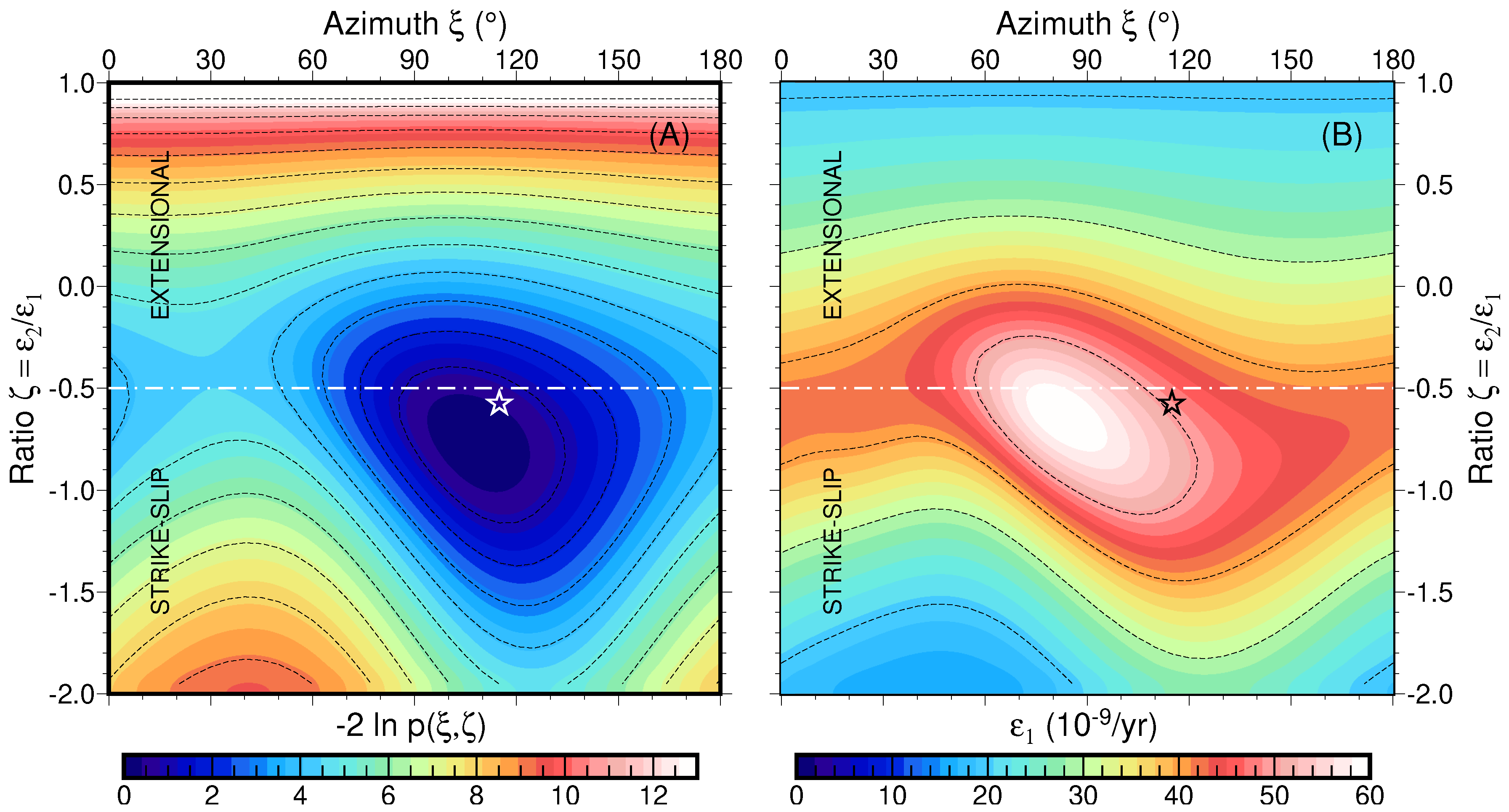
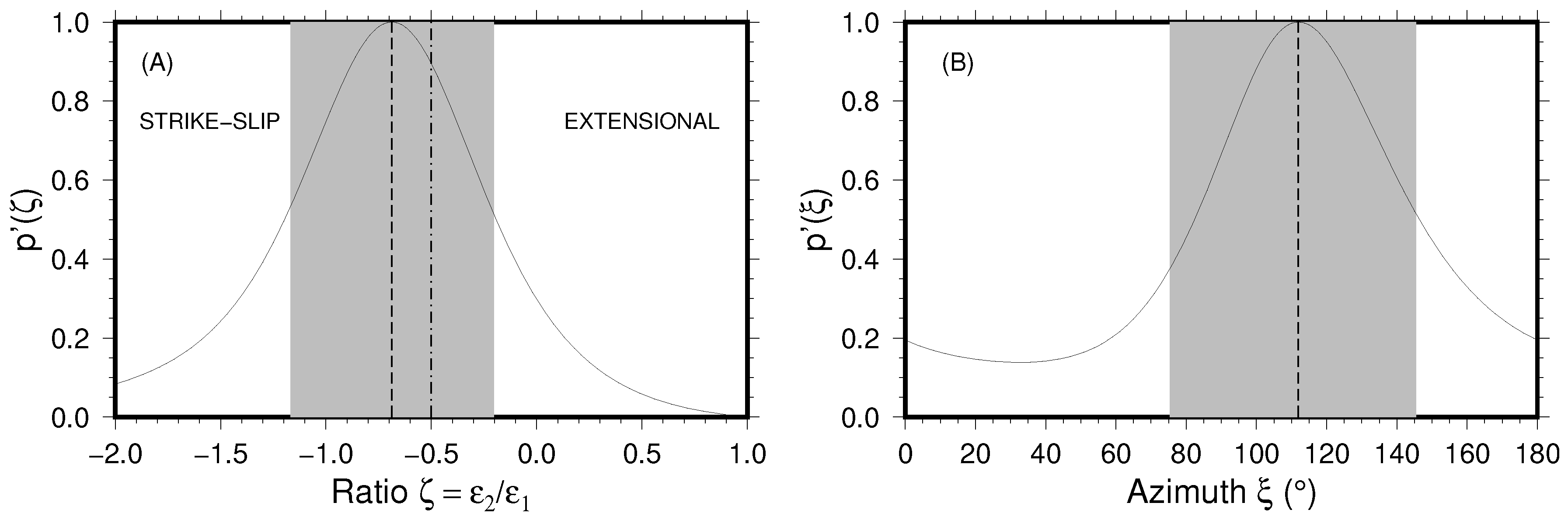
3.3. Prior Information on the Tectonic Regimes

After some minor modifications, the present inverse method can be adapted to include prior information about the tectonic regime and its orientation. For the case of the regional deformation, two principal axes of the deviatoric strain rates, say ${\widehat{\mathbf{x}}}_1$ and ${\widehat{\mathbf{x}}}_2$, are parallel to the Earth surface and the third one, say ${\widehat{\mathbf{x}}}_3$, is perpendicular to it. Denoting with ${ϵ}_i^{\prime }$ the principal value associated with the i-th principal axis and ordering the first two directions in such a way that ${ϵ}_1^{\prime }>{ϵ}_2^{\prime }$, we can discriminate different tectonic regimes according to the following inequalities

$$\begin{array}{ccc}{ϵ}_3^{\prime }<{ϵ}_2^{\prime }<{ϵ}_1^{\prime }\hfill & & \mathrm{extensional}\\ {ϵ}_2^{\prime }<{ϵ}_1^{\prime }<{ϵ}_3^{\prime }\hfill & & \mathrm{compressional}\\ {ϵ}_2^{\prime }<{ϵ}_3^{\prime }<{ϵ}_1^{\prime }\hfill & & \mathrm{strike}-\mathrm{slip}\end{array}$$

(29)

that, using ${ϵ}_3^{\prime }=-{ϵ}_1^{\prime }-{ϵ}_2^{\prime }$, become

$$\begin{array}{ccc}-\frac{1}{2}{ϵ}_1^{\prime }<{ϵ}_2^{\prime }<{ϵ}_1^{\prime }& & \mathrm{extensional}\\ {ϵ}_2^{\prime }<-2{ϵ}_1^{\prime }& & \mathrm{compressional}\\ -2{ϵ}_1^{\prime }<{ϵ}_2^{\prime }<-\frac{1}{2}{ϵ}_1^{\prime }& & \mathrm{strike}-\mathrm{slip}\end{array}$$

(30)

We note that extensional and strike-slip regimes imply ${ϵ}_1^{\prime }>0$, while compressional regimes do not, and that the intermediate principal values for extensional, compressional and strike-slip regimes are ${ϵ}_2^{\prime }$, ${ϵ}_1^{\prime }$ and ${ϵ}_3^{\prime }$, respectively. Furthermore, the direction of maximum extension is ${\widehat{\mathbf{x}}}_1$ for extensional and strike-slip regimes, while the direction of maximum compression is ${\widehat{\mathbf{x}}}_2$ for compressional regimes.

Within this framework, instead of the deviatoric regional strain rates, Equation (8), we can choose the following set of three parameters which make straightforward to recognise the tectonic regimes

$${\mathbf{q}}^{\prime }=\left(\begin{array}{c}{ϵ}_1^{\prime }\\ \zeta \\ \xi \end{array}\right)$$

(31)

where $\xi$ is the azimuth of the first principal direction, ${\widehat{\mathbf{x}}}_1$, and $\zeta ={ϵ}_2^{\prime }/{ϵ}_1^{\prime }$ is the ratio between the two horizontal principal values. After some straigtforward algebra, we can obtain the following relation between the old and new model parameters

$$\mathbf{q}\left({\mathbf{q}}^{\prime }\right)=\widehat{\mathbf{q}}(\zeta ,\xi ){ϵ}_1^{\prime }$$

(32)

with

$$\widehat{\mathbf{q}}(\xi ,\zeta )=\left(\begin{array}{c}{cos}^2\xi +\zeta {sin}^2\xi \\ {sin}^2\xi +\zeta {cos}^2\xi \\ (1-\zeta )sin\xi cos\xi \end{array}\right)$$

(33)

The model space for ${\mathbf{q}}^{\prime }$ is given by

$${\mathcal{Q}}^{\prime }={\mathcal{Q}}_E^{\prime }\cup {\mathcal{Q}}_C^{\prime }\cup {\mathcal{Q}}_S^{\prime }\subset {\mathbb{R}}^3$$

(34)

where ${\mathcal{Q}}_E^{\prime }$, ${\mathcal{Q}}_C^{\prime }$ and ${\mathcal{Q}}_S^{\prime }$ are the following subsets

$$\begin{array}{c}{\mathcal{Q}}_E^{\prime }=(0,\infty )\times (-1/2,1]\times (0,\pi )\subset {\mathbb{R}}^3,\\ {\mathcal{Q}}_C^{\prime }=(0,\infty )\times (-\infty ,-2]\times (0,\pi )\cup (-\infty ,0)\times [2,\infty )\times (0,\pi )\subset {\mathbb{R}}^3,\\ {\mathcal{Q}}_S^{\prime }=(0,\infty )\times (-2,-1/2)\times (0,\pi )\subset {\mathbb{R}}^3\end{array}$$

(35)

which correspond to all the possible model parameters ${\mathbf{q}}^{\prime }$ describing extensional, compressional and strike-slip tectonic regimes, respectively.

Due to the non linearity of Equation (32), the a posteriori PDF modifies according to the Jacobian rule [37]

$$p^{\prime }(\mathbf{w},{\mathbf{q}}^{\prime },{\mathbf{s}}_1,{\mathbf{s}}_2,\mathbf{h})=p(\mathbf{w},\mathbf{q}\left({\mathbf{q}}^{\prime }\right),{\mathbf{s}}_1,{\mathbf{s}}_2,\mathbf{h})J\left({\mathbf{q}}^{\prime }\right)$$

(36)

with

$$J\left({\mathbf{q}}^{\prime }\right)=\left|(1-\zeta ){{ϵ}_1^{\prime }}^2\right|$$

(37)

This form of the a posteriori PDF can be used both to investigate the probabilities of different tectonic regimes, depending directly on the new parameters which make straightforward to recognise the tectonic regimes to which they refer (particularly $\xi$ and $\zeta$), and to include prior information on the tectonic regime by multiplying it with a priori PDF as function of these new parameters or, more simply, investigating the a posteriori PDF over a specific subset of model space ${\mathcal{Q}}^{\prime }$ given in Equation (34).

4. Results

To disclose the behaviour of the long-lasting quiescent Castrovillari normal fault, a campaign GNSS network composed by 10 sites over an area of about $30\mathrm{km}\times 17\mathrm{km}$ centred on the normal-faulting area has thus been set up [25]. Implementation of the campaign sites was carefully performed to ensure a submillimetre forced centring and antenna height measurements. The GNSS measurements started in 2003 and five campaigns have been performed up to 2008. Annual occupations coincided with the September-October (dry) period in an effort to minimize seasonal effects. To avoid displacement artifacts that can be introduced via differing receiver/antenna, all measurements throughout the six-year experiment were performed by using the same instrumentation set-up. During each campaign, data were collected over a period of four consecutive days, with daily sessions of at least 8 h; some network sites have been observed continuously during each period.

Table 2. Site id, longitude, latitude, east and north component of estimated GNSS velocities and relative uncertainties (in mm/yr) used in this study. The original GNSS velocities from Sabadini et al. [25] have been transformed from IGS05 to IGS08 and, then, rotated into an Apulia fixed reference frame [33].

GNSS Data
CASS	16.31969	39.78493	1.33	4.95	0.34	0.18
COLO	16.15402	39.88887	0.99	4.14	0.31	0.37
CROC	16.17953	39.83458	1.07	4.24	0.32	0.31
DOLC	16.25764	39.75962	1.14	4.45	0.44	0.31
DORM	16.29699	39.88124	2.16	4.05	0.39	0.34
FRAN	16.38424	39.82068	3.03	4.46	0.52	0.33
FRAS	16.25836	39.82188	0.45	4.45	0.36	0.33
MORA	16.15572	39.85936	1.18	3.94	0.32	0.28
ZACC	16.16781	39.77370	1.26	4.44	0.50	0.31
CIVI	16.31628	39.82693	4.54	4.05	0.48	0.32

reports the GNSS velocities by Sabadini et al. [25] after transformation from IGS05 to IGS08 and rotation into an Apulia fixed reference frame [33] in order to better highlight the peculiar deformation pattern of the area (Figure 1). Despite the fact that the local GNSS campaigns were carried out for investigating the Castrovillari fault, it guarantees some coverage of the nearby Pollino fault and, so, we extend the present analysis also to the latter. The CIVI, DORM and FRAN stations, indeed, fall within the foot-walls of both faults, while the other stations are above them, mainly in the hanging-walls.

In the following discussion, observed and modelled velocities will be compared in the local fixed reference frame, i.e., after the removal of the rigid body motion estimated by the GNSS data inversions themselves

$$\delta \mathbf{v}(\varphi ,\theta )=\mathbf{v}(\varphi ,\theta )-\mathbf{Q}(\varphi ,\theta )\mathbf{w}$$

(38)

The reference point with respect to which we perform the Taylor expansion of the regional velocity field is $({\varphi }_0,{\theta }_0)=({16.23}^{°},{39.81}^{°})$, about in the middle of the GNSS network.

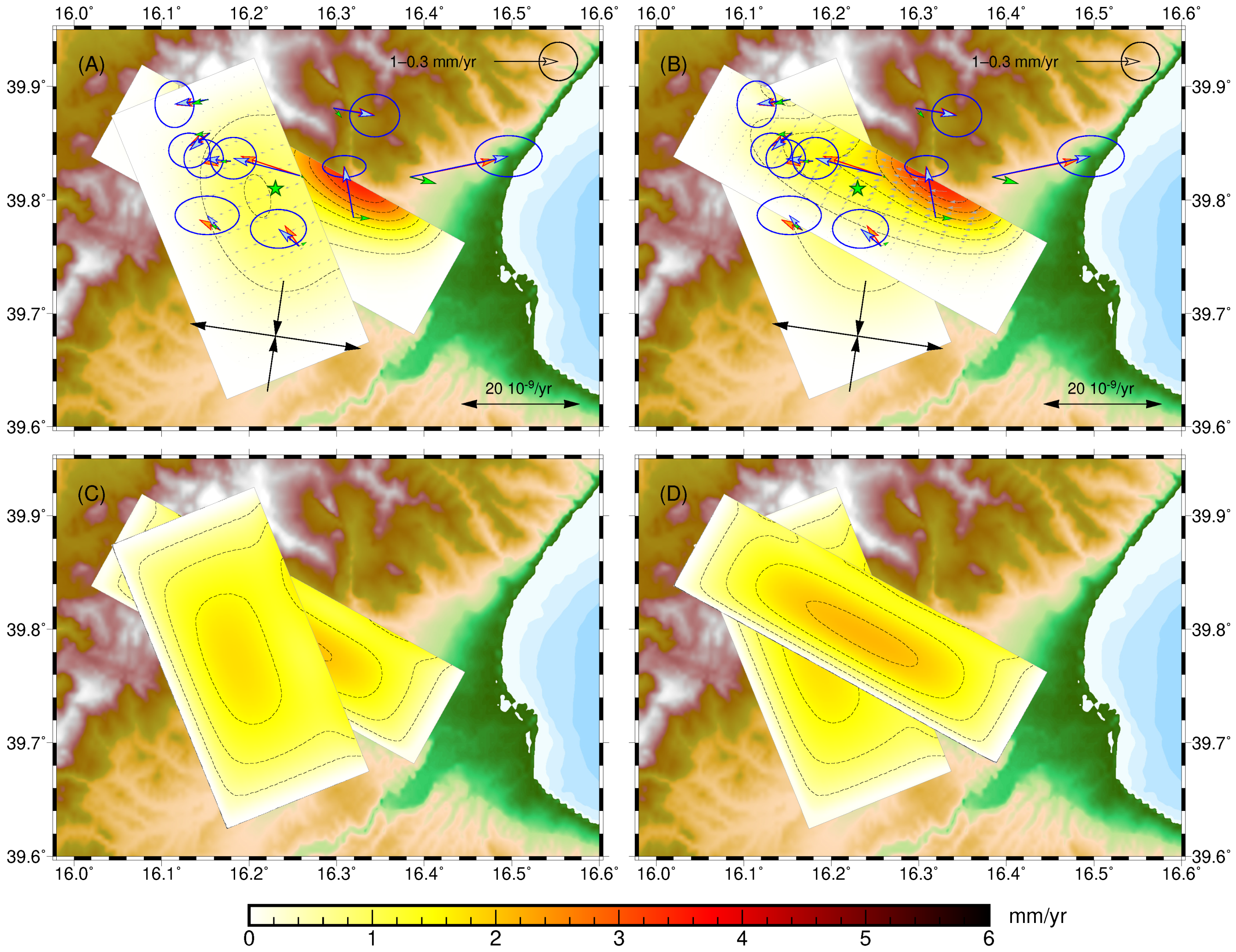
4.1. Regional Deformations without Fault Creep

To provide a first upper bound for the regional deformation, let us first implement the inversion scheme presented in Section 3 for estimating only the regional deformation, i.e., assuming no fault creep. In other words, we investigate the a posteriori PDF given zero fault creep, $p(\mathbf{w},\mathbf{q},\alpha ,\rho )=p(\mathbf{m},\mathbf{h}|{\mathbf{s}}_1={\mathbf{s}}_2=\mathbf{0})$.

Table 3. The mean estimates and standard deviations of the east, $v_{\varphi }$, and north, $v_{\theta }$, components of the regional velocity (in $\mathrm{mm}/\mathrm{yr}$) at the the reference point $({16.23}^{°},{39.81}^{°})$, of the rotation rate, $\omega$ (in ${10}^{-9}/\mathrm{yr}$) and of the mean components of the deviatoric strain rates ${ϵ}_{11}^{\prime }$, ${ϵ}_{22}^{\prime }$ and ${ϵ}_{12}^{\prime }$ (in ${10}^{-9}/\mathrm{yr}$) with respect to the two horizontal principal axes, ${ϵ}_{ij}^{\prime }={\widehat{\mathbf{x}}}_i·{ϵ}^{\prime }·{\widehat{\mathbf{x}}}_j$ ($i,j=1,2$). The results are presented for the different case of GNSS data inversion considered in the main text, with and without fault creep and with prior information about the tectonic regime and the azimuth of the direction of maximum extension, $\xi$. For the inversion schemes R* and FR* the CIVI station is not used.

		Inversion Scheme
	Nickname	R	FR	FR-E${}_{\mathbf{77}}$	FR-E${}_{\mathbf{115}}$	R*	FR*
Features	Creep	no	yes	yes	yes	no	yes
	Regime	all	all	Extensional	Extensional	all	all
	Azimuth	all	all	${77.1}^{°}$	${115.0}^{°}$	all	all
Estimates	$\alpha$	4.75	1.10	1.32	1.05	2.11	0.46
	$v_{\varphi }$	$-0.43\pm 0.30$	$-0.13\pm 0.28$	$-0.18\pm 0.26$	$-0.08\pm 0.24$	$-0.57\pm 0.20$	$-0.28\pm 0.23$
	$v_{\theta }$	$0.49\pm 0.21$	$0.15\pm 0.27$	$0.25\pm 0.26$	$0.19\pm 0.24$	$0.51\pm 0.14$	$0.26\pm 0.22$
	$\omega$	$-10.8\pm 34.6$	$-0.2\pm 32.5$	$-9.7\pm 29.9$	$2.3\pm 29.0$	$-3.0\pm 23.5$	$-0.9\pm 24.0$
	${ϵ}_1^{\prime }$	$86.5\pm 41.2$	$24.2\pm 27.6$	$47.7\pm 25.8$	$40.2\pm 18.9$	$63.9\pm 29.0$	$29.1\pm 22.2$
	${ϵ}_2^{\prime }$	$-62.3\pm 36.3$	$-13.9\pm 31.0$	$-11.0\pm 14.5$	$-9.9\pm 11.5$	$-54.1\pm 24.8$	$-18.9\pm 23.5$
	${ϵ}_{12}^{\prime }$	$0\pm 29.9$	$0\pm 26.8$	0	0	$0\pm 20.2$	$0\pm 20.8$
	$\xi$	${77.1}^{°}$	${115.0}^{°}$	${77.1}^{°}$	${115.0}^{°}$	${74.6}^{°}$	${98.4}^{°}$
		Figure 3A	Figure 4	Figure 8	Figure 9	Figure 3B	Figure 5

(scheme R) lists the mean and standard deviation for the model parameters of the regional deformation, and Figure 3A shows the comparison between observed and modelled surface velocities. The estimated strain rate is primarily consistent with a strike-slip tectonic regime, with WSW-ENE extension of $86.5\pm 41.2\times {10}^{-9}/\mathrm{yr}$ and a slightly smaller compression of $-62.3\pm 36.3\times {10}^{-9}/\mathrm{yr}$ along the perpendicular direction. The large uncertainties of this estimate, nevertheless, does not rule out the possibility of an extensional tectonic regime. The direction of maximum extension is consistent with the large scale deformation pattern estimated by Devoti et al. [38] for this area and, at smaller spatial scales, a little further north in the Pollino Range, by Cheloni et al. [18]. On the other hand, our estimate is more than twice greater than those of these authors (a few tens of nanostrain per year and $34\pm 7\times {10}^{-9}$, respectively). This discrepancy can be explained by considering that our larger estimate has been obtained using a local GNSS network, with GNSS stations close to fault traces and both in the hanging and foot walls of the Castrovillari and Pollino faults, and, so, it is more sensitive to near-field deformations caused by the fault creep rather than just to the regional deformation. In other words, this preliminary result, together with the low seismic activity of the Castrovillari and Pollino faults in the past millenium and the low P- and S-wave velocities of the surrounding area Figure 2; [23,28], indicate that most of this high geodetic strain rate must be accommodated by long-lasting fault creep, at least from 2003 up to 2008 and ever earlier in time, since 1995, as it results by the campaign GNSS network and DInSAR data [25].

An additional indication that these two faults are creeping comes from the fact that the regional deformation alone hardly explain the surface velocities observed by the FRAS and CIVI stations. In particular, even after the removal of the rigid-body motion, the observed velocity for CIVI station is still high, almost $3\mathrm{mm}/\mathrm{yr}$, while the modelled one is less than $1\mathrm{mm}/\mathrm{yr}$. These large discrepancies between observed and modelled ones make large also the estimate of the hyper-parameter $\alpha =4.75$, meaning that modelling errors are still large and, then, motivating the possibility of fault creep in order to improve the modelling of the observed GNSS velocities.

To understand how much the CIVI station affects our results, we performed the same GNSS data inversion without using this station (see Table 3, scheme R*, and Figure 3B). Even in this case the regional deformation alone hardly explain the surface velocities observed at two GNSS stations (now FRAS and FRAN) and the estimate of the hyper-parameter $\alpha =2.11$, although smaller, still indicates the presence of modelling errors. The direction of maximum extension is almost unchanged ($\xi =74.6$) and the maximum strain rate is $63.9\pm 29.0\times {10}^{-9}/\mathrm{yr}$, smaller than the previous one by only the 25 per cent. This result, in addition to confirm the necessity of allowing fault creep, enlightens the role of the CIVI station. Further checks on the impact of this station on our conclusions will be considered in the following discussion.

4.2. Regional Deformations and Fault Creep

Let us now consider the full inversion scheme, where observed surface velocities are explained by both regional deformations and fault creep over the Castrovillari and Pollino faults. Table 3 (scheme FR) lists the mean and standard deviation for the model parameters of the regional deformation, and Figure 4 shows the comparison between observed and modelled surface velocities (blue and orange arrows, respectively), as well as the fault creep distribution and its standard deviation. The contribution to the modelled velocities due to only the regional strain is also shown (green arrows). The estimated strain rates, together with their uncertainties, are consistent with both extensional and strike-slip tectonic regimes, with WNW-ESE extension of $24.2\pm 27.6\times {10}^{-9}/\mathrm{yr}$ and a compression of $-13.9\pm 31.0\times {10}^{-9}/\mathrm{yr}$ along the perpendicular direction (that is about an half of the extension rate in amplitude). The direction of maximum extension is now ${115}^{°}$, rotated of about ${38}^{°}$ clockwise with respect to that estimated by the inversion scheme R. This refined estimate of the regional strain rate, based on the FR inversion scheme rather than the R one, corroborates the transitional character of the investigated area enlightened by the analysis of the focal mechanism from waveform inversion, separating the WSW-ENE extensional domain of the southern Apennines from the NW-SE extensional one of the Calabrian Arc [39,40].

The fault creep distributions for the Castrovillari and Pollino faults indicate a normal/right-lateral strike-slip mechanism with average rake angle of $-{126}^{°}$ and $-{143}^{°}$ and maxima of $2.1\mathrm{mm}/\mathrm{yr}$ and $5.2\mathrm{mm}/\mathrm{yr}$ close to the fault traces, in correspondence with the FRAS and CIVI stations, respectively. The standard deviation for both the fault creep distribution is about 2∼3 $\mathrm{mm}/\mathrm{yr}$ and goes to zero at the internal edges due to the a priori constraints that the fault creep distribution is zero outside the adopted rectangular areas. In light of this, we can assess that the fault creep on the Pollino fault is statistically significant (i.e., it differs from zero by about two-sigma errors), while that on the Castrovillari fault is not (it is about one-sigma error).

Comparing Figure 3 and Figure 4, we note that the observed and modelled velocities are in better agreement for the inversion scheme FR than they are for the inversion scheme R. This results also from the estimate of the hyper-parameter $\alpha$, that is now $\alpha =1.10$ instead of $\alpha =4.75$ (see Table 3), meaning that the discrepancies between observed and modelled velocities are consistent with the observational errors, while the modelling errors are negligible. This reduction of the hyper-parameter $\alpha$ confirms the fact that fault creep is the necessary physical mechanism in order to explain the velocity changes on the small spatial scale of the campaign GNSS network. On the other hand, different from Sabadini et al. [25], our updated results indicate that the creep is mainly occurring on the Pollino fault rather than the Castrovillari fault, which was the only fault considered in this previous study. Furthermore, we note that the observed velocities are mainly explained by the fault creep rather than by the regional deformation. The contribution to surface velocities due to the regional strain rate (green arrows), indeed, is only a small fraction of the modelled velocities which also include the contribution from the fault creep (orange arrows) and, in amplitude, is smaller than the one-sigma errors affecting the observed surface velocities. This fact thus explains why the estimated regional strain rate is consistent with the case of no regional strain (the maximum extension rate of $24.2\times {10}^{-9}/\mathrm{yr}$ is indeed smaller than its one-sigma error of $27.6\times {10}^{-9}/\mathrm{yr}$) and points out how the large variations of the observed surface velocities from one GNSS station to another of the local GNSS campaign network are mainly due to fault creep, at least on the Pollino fault.

Our estimates, both of the regional strain rates and of the fault creep distributions, are affected by large uncertainties due to the small number of GNSS data used in the inversion, as well as due to the smallness of the geographical area that they cover. Increasing the number of GNSS station would certainly decrease these uncertainties and, particularly, improve the resolving power on the fault creep distribution. Enlarging the covered geographic area, instead, would affect mainly the estimate of the regional deformation because larger baseline lengths between GNSS stations better constrain large spatial scale strain rates. On the other hand, they could be affected by deformation caused by other creeping faults other than those here considered. Furthermore, regional strain rates could vary on larger spatial scales, making more inaccurate the first-order expansion of the regional velocity field, Equation (2). Therefore, in this first attempt to discriminate intraplate regional deformation from fault creep, we have preferred to consider only the campaign GNSS network by Sabadini et al. [25], without adding complexities such as including additional GNSS stations from other GNSS networks far away from the near-field of the Pollino and Castrovillari faults.

An even more stringent issue that prevent us from including additional data in the present analysis is that all the permanent GNSS stations in the proximity of the Pollino and Castrovillari faults were set up only in recent years. In this respect, these additional observed crustal velocities would refer to time periods different (and without overlapping) from that of the GNSS campaign used here and they thus reflect averaged fault creep which can be different from that occurring during the six year GNSS campaign (2003–2008). Significant variations in the fault creeps over the years have to be expected due to transient aseismic processes as, for instance, the one observed by Cheloni et al. [18] from 2010 to 2014, a little further north to the Pollino and Castrovillari faults. Because our inverse method aims at estimating the long-term trend due to aseismic processes in a specific time windows and it does not take into account their evolution in time, these variations from one time periods to another would introduce modelling errors that biases the estimate of a hardly quantifiable amount. Further improvements in the understanding of complex spatial pattern and temporal evolution of displacement time series at intraplate regions can be achieved in the future by combining our method, based on the discrimination of the spatial patterns of the different physical processes, with the classical ones, mainly based on the alone temporal evolution.

As already done in Section 4.1 about the effects of the CIVI station on the estimate of the only regional deformation, we performed the same GNSS data inversion for estimating both regional deformation and fault creep without using this station (see Table 3, scheme FR*, and Figure 5). The estimate of the regional strain rate is slightly larger than that obtained within the inversion scheme FR (the maximum extension and compression are $29.1\pm 22.2\times {10}^{-9}/\mathrm{yr}$ and $-18.9\pm 23.5\times {10}^{-9}/\mathrm{yr}$ instead of $24.2\pm 27.6\times {10}^{-9}/\mathrm{yr}$ and $-13.9\pm 31.0\times {10}^{-9}/\mathrm{yr}$) and the direction of maximum extension is slightly rotated anti-clockwise by about ${17}^{°}$ ($\xi ={98.4}^{°}$ instead of ${115.0}^{°}$). Furthermore, the fault creep distribution over the Castrovillari fault is twice smaller, with the shallow maximum of $1.0\mathrm{mm}/\mathrm{yr}$ instead of $2.1\mathrm{mm}/\mathrm{yr}$, while that over the Pollino fault decreases by about the 30 per cent, with the shallow maximum of $3.5\mathrm{mm}/\mathrm{yr}$ instead of $5.2\mathrm{mm}/\mathrm{yr}$. These differences in the estimates, when compared with their uncertainties, are minor and the same main considerations based on the inversion scheme FR still hold even if the CIVI station is not used in the inversion. In particular, the normal/right-lateral strike-slip mechanism of the Pollino fault is confirmed also by the inversion scheme FR* and the regional strain rate are consistent with both strike-slip and normal tectonic regimes, with a maximum extension of about a few tens of nanostrain per year.

In contrast to the inversion scheme FR where the agreement between observed and modelled GNSS velocities is consistent with observational errors from GNSS data processing, the inversion scheme FR* yields a smaller estimate of the hyper-parameter $\alpha$, that is now $\alpha =0.46$ instead of $\alpha =1.10$, meaning that the model fits too well the GNSS velocities. This fact can be seen as an indication that observational errors have been overestimated during the GNSS data processing or that the model is overparameterized compared to the few data at our disposal. As already mentioned above and as reminder for next local GNSS campaigns, a denser GNSS network will certainly improve our results, making them less sensitive to single GNSS stations.

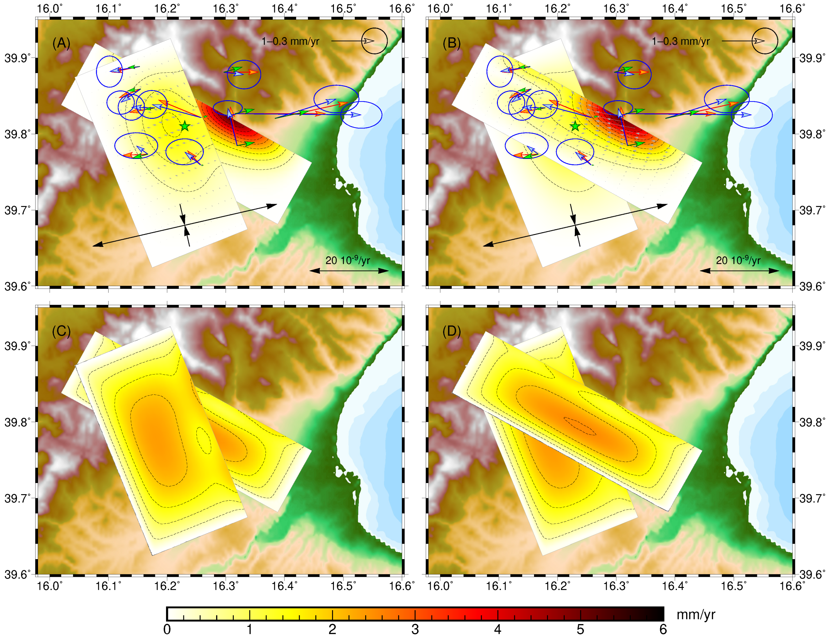
4.3. Regional Deformations and Fault Creep and Prior Information about the Tectonic Regimes

To better understand the results obtained from the inversion scheme FR and, at the same time, to enlighten the full potential of our novel inverse method, let us now consider the inclusion of prior information about the tectonic regimes as described in Section 3.3.

Figure 6A shows the marginal PDF for extensional and strike-slip tectonic regimes, varying both the azimuth of the maximum extension direction, $\xi$, and the ratio between the two horizontal principal values, $\zeta$,

$$p^{\prime }(\xi ,\zeta )={\int }_0^{\infty }\left({\int }_{\mathcal{W}\times {\mathcal{S}}_1\times {\mathcal{S}}_2}^{}{p}^{\prime }(\mathbf{w},{\mathbf{q}}^{\prime },{\mathbf{s}}_1,{\mathbf{s}}_2,\mathbf{h})\mathrm{d}\mathbf{w}\mathrm{d}{\mathbf{s}}_1\mathrm{d}{\mathbf{s}}_2\mathrm{d}\mathbf{h}\right)\mathrm{d}{ϵ}_1^{\prime }$$

(39)

with $p^{\prime }(\mathbf{w},{\mathbf{q}}^{\prime },{\mathbf{s}}_1,{\mathbf{s}}_2,\mathbf{h})$ being given by Equation (36). We have not considered compressional tectonic regimes because both the inversion schemes R and FR have already shown that it is the less likely one. In Figure 6B, instead, we report the maximum extension rate estimated varying the tectonic regimes. The marginal PDFs for the only ratio between the two horizontal principal values, $\zeta$,

$$p^{\prime }\left(\zeta \right)={\int }_0^{\pi }{p}^{\prime }(\xi ,\zeta )\mathrm{d}\xi$$

(40)

and the only azimuth of the maximum extension direction, $\xi$,

$$p^{\prime }\left(\xi \right)={\int }_{-2}^1{p}^{\prime }(\xi ,\zeta )\mathrm{d}\zeta$$

(41)

are shown in Figure 7.

The marginal PDF has its maximum close to the tectonic regime estimated within the inversion scheme FR ($\xi ={115}^{°}$ and $\zeta =-0.57$) and it is bell shaped, but for some asymmetries across the transition from strike-slip to normal tectonic regimes. We note also that the strike-slip tectonic regimes are more likely than the normal ones, although the latter cannot be excluded. The different location of the maximum of the marginal PDF and the tectonic regime estimated by the inversion scheme FR is attributable to the different meaning of the two approaches, with and without prior information about the tectonic regimes. Indeed, within the inversion scheme FR, the tectonic regime is inferred by the mean strain rate tensor (which can be seen as it has been obtained by averaging the strain rate tensors for every tectonic regimes weighted by their probabilities), while the marginal PDF is obtained by considering each tectonic regime separately. This difference also explains why the maximum extension rate of $24.2\times {10}^{-9}/\mathrm{yr}$ estimated within the inversion scheme FR is twice smaller than the maximum extension rate estimated using the same tectonic regime inferred from the inversion scheme FR as prior information (see the value in correspondence of the black star in Figure 6B that is about $50\times {10}^{-9}/\mathrm{yr}$). However, as shown in Figure 6B, it is noteworthy to notice that the maximum extension rate for the normal and strike-slip tectonic regimes is always smaller than $60\times {10}^{-9}/\mathrm{yr}$ and therefore even smaller than the estimate of $86.5\times {10}^{-9}/\mathrm{yr}$ obtained within the inversion scheme R, when the fault creep is not allowed.

As shown in Figure 7, from the marginal PDFs for the only ratio between the two horizontal principal values, $\zeta$, and the only azimuth of the maximum extension direction, $\xi$, we can quantify the 68 per cent confidence intervals (grey regions), which are $\zeta \in [-1.167,-0.202]$ and $\xi \in [75.4,145.5]$ or, equivalently, $\zeta =-{0.687}_{-0.480}^{+0.485}$ and $\xi ={{112.0}^{°}}_{-36.5}^{+33.5}$, with $\zeta =-0.687$ and $\xi ={112.0}^{°}$ being the parameters at which the PDFs have their maxima (vertical dashed lines).

To gain insight on the impact of prior information about the tectonic regimes on the results, we now consider the two representative inversion schemes FR-E${}_{77}$ and FR-E${}_{115}$ where we fix a priori the direction of maximum extension at $\xi ={77.1}^{°}$ and ${115.0}^{°}$, respectively (these are the same azimuths obtained from the inversion schemes R and FR), and we require that the tectonic regime is normal, as commonly expected for the Apennines chain (that is we consider all the ratios between the horizontal principal values from $-1/2$ to 1, $\zeta \in (-1/2,1))$. As before, Table 3 (schemes FR-E${}_{77}$ and FR-E${}_{115}$) lists the mean and standard deviation for the model parameters of the regional deformation, and Figure 8 and Figure 9 show the comparisons between observed and modelled velocities (blue and orange arrows, respectively), as well as the fault creep distributions and their standard deviation.

We note that the fault creep distributions are not affected by the inclusion of the prior information about the tectonic regime, with the exception of some minor differences which are smaller than the uncertainties as, for instance, the smaller creep obtained over the Castrovillari fault, with a deeper maximum of about $1.6\mathrm{mm}/\mathrm{yr}$. The contribution from the regional strain rate to the modelled surface velocities (green arrows), instead, is greater than that obtained within the inversion scheme FR and, indeed, the estimates of the maximum extension rate ($46.8$ and $40.0\times {10}^{-9}/\mathrm{yr}$ for the inversion schemes FR-E${}_{77}$ and FR-E${}_{115}$, respectively) is about twice larger than that for the inversion scheme FR without prior information. Nevertheless, as noticed above, this increase in the estimated extension rates must be ascribed to the fact that the same estimate with the inversion scheme without prior information results from a weighted average of the strain rate tensors of every tectonic regimes which, differing in the direction of maximum extension, compensate each other to some extent.

5. Discussion

The inverse method presented in Section 3 have been adopted to explain the surface horizontal velocities obtained from a six year GNSS campaign [25] over the Castrovillari and Pollino faults, cutting the southern portion of the Pollino seismic gap [20]. Achieved results have provided valuable information on the regional deformation of the area and on the aseismic processes occurring on both faults. More in detail, the model where only the regional deformation is considered (i.e., the scheme R) yields large residuals between modelled and observed velocities, larger by more than two times the observational uncertainties (see Figure 3 and the estimate of the hyper-parameter $\alpha$ reported in Table 3). Different, when the fault creep is allowed (i.e., the scheme FR), the residuals become consistent with the observational uncertainties (see Figure 4 and again Table 3), indicating that a more sophisticated model is necessary for explaining the observations. In particular, this second inversion clearly indicates, above the estimated uncertainties, that the Pollino fault is creeping, with a maximum slip rate of $5.2\mathrm{mm}/\mathrm{yr}$ one. The six year GNSS campaign, indeed, points out that the largest velocities occur at those GNSS sites close to the Pollino fault trace (marked by blue line in Figure 1) and that such a spatial pattern can be hardly explained only on the basis of a regional deformation. Moreover, such a creeping behavior of the Pollino fault, while confirm the results achieved in Sabadini et al. [25], are well supported by the seismic observations which identified it as a low P- and S-wave velocity crustal zone (see Figure 1), therefore suggesting an anomalous thermal state of the crust. This anomalous thermal state of the crust would inhibit frictional fault sliding in favour of creeping deformation, as testified by the lack of large earthquakes (M > 6) in the last centuries.

The limitations due to the number and the geographical distribution of the adopted GNSS sites, nevertheless, does not allow us to constrain the regional deformation with high accuracy. In particular, it remains an ambiguity between extensional or strike-slip tectonic regimes, although the latter is slightly more likely as shown in Figure 7A. The inversion scheme FR, indeed, yields a maximum extension of $24.2\pm 27.6/\mathrm{yr}$ with an azimuth of ${115}^{°}$ and maximum compression of $-13.9\pm 31/\mathrm{yr}$ along the perpendicular direction. In light of this, although the estimated regional deformation is characterized by high uncertainties of the order of a few tens of nanostrain per year (comparable with the expected value of strain rate in southern Italy), the data from the GNSS measurements, jointly with the novel inverse method, support the hypothesis of fault creeping, at least as it concerns the Pollino fault. Improvements in the estimate of the model parameters will be achieved in the future by exploiting more data and planning their spatial distribution on the basis of synthetic tests performed within the framework of the present inverse method. Furthermore, the planning of additional GNSS campaign measurements of the existing GNSS episodic network will benefit of the increasing number of continuous GNSS stations installed in the area since the past decade. As already argued in Section 4.2, it will be important to guarantee the overlapping of the time intervals spanned by continuous and campaign GNSS stations. Indeed, the present inverse method, being based on the crustal velocities over a specific time interval, can only provide an estimate of the average fault creep over the same time interval.

To verify the sensitivity of our results to specific GNSS stations, we have performed a similar inversion (i.e., the scheme FR*) removing the CIVI station, which presents the largest velocity in the Apulia fixed reference frame. The results are similar to that obtained using all the data (i.e, the scheme FR) but for the fact that the estimated regional strain rate is slightly larger (the maximum extension and compression are $29.1\pm 22.2\times {10}^{-9}/\mathrm{yr}$ and $-18.9\pm 23.5\times {10}^{-9}/\mathrm{yr}$ instead of $24.2\pm 27.6\times {10}^{-9}/\mathrm{yr}$ and $-13.9\pm 31.0\times {10}^{-9}/\mathrm{yr}$) and the Pollino fault creep decreases by about the 30 per cent, with the shallow maximum of $3.5\mathrm{mm}/\mathrm{yr}$ instead of $5.2\mathrm{mm}/\mathrm{yr}$. Furthermore, in order to consider the possibility of including prior information about the tectonic regime, we have discussed the estimates obtained requiring that a normal tectonic regime and fixing the direction of maximum extension with the azimuth obtained by the inversion scheme R and FR.

6. Conclusions

We have developed a novel inverse method for discriminating regional deformation and fault creep from surface velocities observed by a GNSS network at the spatial scale of intraplate faults which allows including, or not, prior information on the tectonic regime. Surface velocities caused by the fault creep are modelled according to the dislocation theory e.g., [32] while the rigid-body motion and regional strain rates describing the regional deformation are assumed to be homogeneous in space and dealt with as additional model parameters [30]. Then, we have applied this inverse method for explaining the surface velocities obtained from the GNSS network over the Castrovillari and Pollino faults [25].

In contrast to other studies which only focus on transient aseismic processes [18], this method allows us to estimate the whole fault creep over the time window spanned by the GNSS time series within intraplate areas. This is a crucial advancement because it allows us to deal even with cases of long-lasting creep of intraplate faults, the effects of which are linear in time and consequently they cannot be easily discriminated by the secular trends due to regional strain rates on the basis of time series analyses. They are herein rather discriminated by exploiting the different spatial signatures of the regional deformation (homogeneous in space when the investigated area is small and does not exceed the typical spatial scales at which tectonic processes change, generally fifty to hundred kilometres) and of the fault creep (localised in the near-field of the creeping faults). In light of this, the present inverse method is effective in recognizing creeping faults by jointly estimating the fault creep distribution and regional strain rates, as well as the rigid-body motion of the investigated area. In doing so, our estimated regional strain rate constitutes a refinement of the upper bound of the strain accumulation process presently based on the geodetic strain rate, including the main aseismic processes affecting the crust sampled by the GNSS network.

In this respect, taking advantages of the different spatial signatures of the main physical mechanism responsible for crustal displacements, the present method complements the already available methods which aim to detect departures from linear trends in the GNSS time series and interpret them in terms of effects of transient fault creeps. Further improvements in the understanding of the complex spatial pattern and temporal evolution of displacement time series in intraplate regions, where both transient and long-term aseismic processes can be relevant, will be obtained by combining this method with the previous ones mainly based on the alone temporal evolution.

For the case study here considered, the southern portion of the Pollino seismic gap, the geodetic strain rate estimated by the observed GNSS velocities is characterized by a maximum extension rate of about $86.5\times {10}^{-9}/\mathrm{yr}$, as it results from the inversion scheme R which does not account for any aseismic processes. Allowing for the possibilities of fault creep over both the Castrovillari and Pollino faults in the inversion scheme R, this estimate is reduced by more than 70 per cent, to about $24.2\times {10}^{-9}/\mathrm{yr}$ and the agreement between observed and modelled surface velocities greatly improves mainly due to a normal/right-lateral strike-slip creep of the Pollino fault, with maximum slip rates of about $5\mathrm{mm}/\mathrm{yr}$. This inversion also predicts a smaller creep over the Castrovillari fault, with maximum of $2\mathrm{mm}/\mathrm{yr}$. Nevertheless, despite the Pollino fault, the latter estimate is smaller than its uncertainties and, then, we cannot conclude that also the Castrovillari fault is creeping.

As expected, taking into account the main sources of aseismic deformation, the estimate of the regional strain rate becomes much smaller than the geodetic strain rate obtained within the inversion scheme R. Furthermore, as indicated by the estimate of the hyper-parameter $\alpha$, the modelling of the observed surface velocities greatly improves and the discrepancies between observed and modelled surface velocities are consistent with observational errors, without the need for invoking additional modelling errors. The estimated regional strain rate, nevertheless, is affected by large uncertainties and this makes difficult to assess whether the southern area of the Pollino Range is characterised by a normal or strike-slip tectonic regime, as well as to define accurately its orientation.

The inclusion of prior information about the tectonic regime does not alter significantly the fault creep distributions of the Pollino and Castrovillari faults, but it can double the estimates of maximum extension due to regional deformation, as shown by the two representative inversion schemes FR-E${}_{77}$ and FR-E${}_{115}$. The estimated maximum extensions, however, are still (about twice) smaller than the geodetic strain rate obtained by the inversion scheme R.

Due to the complex tectonic setting of the investigated area, we cannot argue in favour of specific prior information to be used. On the other hand, these results show that it is important to jointly consider regional deformation and aseismic processes in order to correctly interpret crustal motion and that we can obtain novel insights on the regional strain rates, although affected by large uncertainties.

References

1. Clarke, P.J.; Davies, R.R.; England, P.C.; Parsons, B.; Billiris, H.; Paradissis, D.; Veis, G.; Cross, P.A.; Denys, P.H.; Ashkenazi, V.; et al. Crustal strain in central Greece from repeated GPS measurements in the interval 1989–1997. Geophys. J. Int. 1998, 135, 195–214. [Google Scholar] [CrossRef] [Green Version]
2. Mazzotti, S.; Leonard, L.; Cassidy, J.; Rogers, G.; Halchuk, S. Seismic hazard in western Canada from GPS strain rates versus earthquake catalog. J. Geophys. Res. 2011, 116, B12310. [Google Scholar] [CrossRef]
3. Palano, M.; Imprescia, P.; Agnon, A.; Gresta, S. An improved evaluation of the seismic/geodetic deformation-rate ratio for the Zagros Fold-and-Thrust collisional belt. Geophys. J. Int. 2018, 213, 194–209. [Google Scholar] [CrossRef]
4. Masson, F.; Chery, J.; Hatzfeld, D.; Martinod, J.; Vernant, P.; Tavakoli, F.; Ghafory-Ashtiani, M. Seismic versus aseismic deformation in Iran inferred from earthquakes and geodetic data. Geophys. J. Int. 2005, 160, 217–226. [Google Scholar] [CrossRef]
5. Savage, J.C.; Burford, R.O. Geodetic determination of relative plate motion in Central California. J. Geophys. Res. 1973, 78, 832–845. [Google Scholar] [CrossRef] [Green Version]
6. Savage, J.C. A dislocation mode of strain accumulation and release at a subduction zone. J. Geophys. Res. 1983, 88, 4984–4996. [Google Scholar] [CrossRef]
7. McCaffrey, R. lnterseismic locking on the Hikurangi subduction zone: Uncertainties from slow-slip events. J. Geophys. Res. 2014, 119, 7874–7888. [Google Scholar] [CrossRef] [Green Version]
8. Li, S.; Moreno, M.; Bedford, J.; Rosenau, M.; Oncken, O. Revisiting viscoelastic effects on interseismic deformation and locking degree: A case study of the Peru-North Chile subduction zone. J. Geophys. Res. 2015, 120, 4522–4538. [Google Scholar] [CrossRef] [Green Version]
9. Ranalli, G. Rheology of the Earth, 2nd ed.; Chapman and Hall: London, UK, 1995. [Google Scholar]
10. Splendore, R.; Marotta, A. Crust-mantle mechanical structure in the Central Mediterranean region. Tectonophysics 2013, 603, 89–103. [Google Scholar] [CrossRef]
11. England, P.; McKenzie, D. A thin viscous sheet model for continental deformation. R. Astron. Soc. Geophys. J. 1982, 70, 295–321, Erratum in 1983, 73, 523–532. [Google Scholar] [CrossRef]
12. Medvedev, S.; Podladchikov, Y. New extended thin-sheet approximation for geodynamic applications–I. Model formulation. Geophys. J. Int. 1999, 136, 567–585. [Google Scholar] [CrossRef] [Green Version]
13. Marotta, A.; Sabadini, R. The signatures of tectonics and glacial isostatic adjustment revealed by the strain rate in Europe. Geophys. J. Int. 2004, 157, 865–870. [Google Scholar] [CrossRef] [Green Version]
14. Marotta, A.; Mitrovica, J.; Sabadini, R.; Milne, G. Combined effects of tectonics and glacial isostatic adjustment on intraplate deformation in central and northern Europe: Applications to geodetic baseline analyses. J. Geophyis. Res. 2004, 109, B01413. [Google Scholar] [CrossRef] [Green Version]
15. Jiménez-Munt, I.; Garcia-Castellanos, D.; Negredo, A.; Platt, J. Gravitational and tectonic forces controlling postcollisional deformation and the present-day stress field of the Alps: Constraints from numerical modeling. Tectonics 2005, 24, TC5009. [Google Scholar] [CrossRef] [Green Version]
16. Hearn, E. What can GPS data tell us about the dynamics of post-seismic deformation? Geophys. J. Int. 2003, 155, 753–777. [Google Scholar] [CrossRef]
17. Hutton, W.; DeMets, C.; Sanchez, O.; Suarez, G.; Stock, J. Slip kinematics and dynamics during and after the 1995 October 9 Mw = 8.0 Colima-Jalisco earthquake, Mexico, from GPS geodetic constraints. Geophys. J. Int. 2001, 146, 637–658. [Google Scholar] [CrossRef] [Green Version]
18. Cheloni, D.; D’Agostino, N.; Selvaggi, G.; Avallone, A.; Fornaro, G.; Giuliani, R.; Reale, D.; Sansosti, E.; Tizzani, P. Aseismic transient during the 2010–2014 seismic swarm: Evidence for longer recurrence of M ≥ 6.5 earthquakes in the Pollino gap (Southern Italy)? Sci. Rep. 2017, 7, 576. [Google Scholar] [CrossRef] [Green Version]
19. Murray, J.; Minson, S.; Svarc, J. Slip rates and spatially variable creep on faults of the northern San Andreas system inferred through Bayesian inversion of Global Positioning System data. J. Geophys. Res. 2014, 119, 6023–6047. [Google Scholar] [CrossRef]
20. Cinti, F.; Moro, M.; Pantosti, D.; Cucci, L.; D’Addezio, G. New constraints on the seismic history of the Castrovillari fault in the Pollino gap (Calabria, southern Italy). J. Seismol. 2002, 6, 199–217. [Google Scholar] [CrossRef]
21. Michetti, A.; Ferreli, L.; Serva, L.; Vittori, E. Geological evidence for strong historical earthquakes in an “aseismic” region: The Pollino case. J. Geodyn. 1997, 24, 67–86. [Google Scholar] [CrossRef]
22. Totaro, C.; Presti, D.; Billi, A.; Gervasi, A.; Orecchio, B.; Guerra, I.; Neri, G. The ongoing seismic sequence at the Pollino Mountains. Italy Seismol. Res. Lett. 2013, 84, 955–962. [Google Scholar] [CrossRef] [Green Version]
23. Totaro, C.; Koulakov, I.; Orecchio, B.; Presti, D. Detailed crustal structure in the area of the southern Apennines–Calabrian Arc border from local earthquake tomography. J. Geodyn. 2014, 82, 87–97. [Google Scholar] [CrossRef]
24. Chiarabba, C.; Agostinetti, N.; Bianchi, I. Lithospheric fault and kinematic decoupling of the Apennines system across the Pollino range. Geophys. Res. Lett. 2016, 43, 3201–3207. [Google Scholar] [CrossRef] [Green Version]
25. Sabadini, R.; Aoudia, A.; Barzaghi, R.; Crippa, B.; Marotta, A.; Borghi, A.; Cannizzaro, L.; Calcagni, L.; Dalla Via, G.; Rossi, G.; et al. First evidences of fast creeping on a long-lasting quiescent earthquake normal-fault in the Mediterranean. Geophys. J. Int. 2009, 179, 720–732. [Google Scholar] [CrossRef] [Green Version]
26. Brozzetti, F.; Cirillo, D.; de Nardis, R.; Cardinali, M.; Lavecchia, G.; Orecchio, B.; Presti, D.; Totaro, C. Newly identified active faults in the Pollino seismic gap, southern Italy, and their seismotectonic significance. J. Struct. Geol. 2017, 94, 13–31. [Google Scholar] [CrossRef] [Green Version]
27. DISS Working Group. Database of Individual Seismogenic Sources (DISS), Version 3.0.4: A Compilation of Potential Sources for Earthquakes Larger than M 5.5 in Italy and Surrounding Areas. 2007. Available online: http://www.ingv.it/DISS/ (accessed on 15 July 2017).
28. Rovida, A.; Camassi, R.; Gasperini, P.; Stucchi, M. CPTI11, la versione 2011 del Catalogo Parametrico dei Terremoti Italiani, Milano, Bologna. 2011. Available online: http://emidius.mi.ingv.it/CPTI (accessed on 15 July 2017).
29. ISIDe Working Group. Italian Seismological Instrumental and Parametric Databases. 2016. Available online: http://cnt.rm.ingv.it/iside (accessed on 15 July 2017).
30. Savage, J.; Gan, W.; Svarc, J. Strain accumulation and rotation in the Eastern California Shear Zone. J. Geophys. Res. 2001, 106, 21995–22007. [Google Scholar] [CrossRef]
31. Shen, Z.K.; Jackson, D.; Ge, B. Crustal deformation across and beyond the Los Angeles basin from geodetic measurements. J. Geophys. Res. 1996, 101, 27957–27980. [Google Scholar] [CrossRef]
32. Okada, Y. Internal deformation due to shear and tensile faults in a half-space. Seismol. Soc. Am. 1992, 82, 1018–1040. [Google Scholar]
33. Ferranti, L.; Palano, M.; Cannavò, F.; Mazzella, M.; Oldow, J.; Gueguen, E.; Mattia, M.; Monaco, C. Rates of geodetic deformation across active faults in southern Italy. Tectonophysics 2014, 621, 101–122. [Google Scholar] [CrossRef]
34. Yabuki, T.; Matsu’ura, M. Geodetic data inversion using a Bayesian information criterion for spatial distribution of fault slip. Geophys. J. Int. 1992, 109, 363–375. [Google Scholar] [CrossRef]
35. Cambiotti, G.; Zhou, X.; Sparacino, F.; Sabadini, R.; Sun, W. Joint estimate of the rupture area and slip distribution of the 2009 L’Aquila earthquake by a Bayesian inversion of GPS data. Geophys. J. Int. 2017, 209, 992–1003. [Google Scholar] [CrossRef] [Green Version]
36. Fukuda, J.; Johnson, K. A fully Bayesian inversion for spatial distribution of fault slip with objective smoothing. Bull. Seism. Soc. Am. 2008, 98, 1128–1146. [Google Scholar] [CrossRef]
37. Tarantola, A. Inverse Problem Theory and Methods for Model Parameter Estimation; SIAM: Philadelphia, PA, USA, 2005. [Google Scholar]
38. Devoti, R.; Esposito, A.; Pietrantonio, G.; Pisani, A.; Riguzzi, F. Evidence of large scale deformation patterns from GPS data in the Italian subduction boundary. EPSL 2011, 311, 230–241. [Google Scholar] [CrossRef]
39. Orecchio, B.; Prestia, D.; Totaro, C.; D’Amico, S.; Neri, G. Investigating slab edge kinematics through seismological data: Thenorthern boundary of the Ionian subduction system (south Italy). J. Geodyn. 2015, 88, 23–35. [Google Scholar] [CrossRef]
40. Totaro, C.; Orecchio, B.; Presti, D.; Scolaro, S.; Neri, G. Seismogenic stress field estimation in the Calabrian Arc region (south Italy) from a Bayesian approach. Geophys. Res. Lett. 2016, 43, 8960–8969. [Google Scholar] [CrossRef]
Figure 1. Surface velocities from the GNSS campaigns (in Apulia fixed reference frame, black arrows) from Sabadini et al. [25], the fault traces (gray, red and blue lines) identified by Brozzetti et al. [26] and the Castrovillari and Pollino faults used in this study (white solid rectangles). Red and blue lines are the fault traces associated with the Castrovillari and Pollino faults, respectively, and the white dashed rectangle indicates the Castrovillari fault from the Database of Individual Seismogenic Sources [27]. The top edge of the DISS fault is slightly shifted southwestward because is at 1 km depth rather than at the Earth surface. The topography of the area is shown in the background and the inset shows the south Italy and the location of the plotted region (red rectangle).
Remotesensing 12 02921 g001
Figure 2. Historical (from 1000 to 1984, blue circles) and recent (from 1895 to present, gray and black circles) earthquakes from the CPTI11 and ISIDe catalogs [28,29]. The velocities of the seismic P-waves at 9 km depth from Totaro et al. [23] are shown in the background.
Remotesensing 12 02921 g002
Figure 3. (A) Comparison between observed and modelled surface velocities (blue and green arrows, respectively) according to the inversion scheme R (see Table 3), after the removal of the estimated rigid-body motion. The ellipses represents the one-sigma errors from GNSS data analysis (observational errors) and should be rescaled by the square root of the estimated hyper-parameter α in order to account for the modelling errors ( α = 2.18 for this inversion). The regional strain rate is also drawn, further south with respect to the reference point ( ϕ 0 , θ 0 ) of the Taylor series expansion (green star). (B) As panel A, but for the inversion scheme R* (see Table 3, α = 1.45 ), where the CIVI station has not been used.
Remotesensing 12 02921 g003
Figure 4. (A,B) Mean fault creep distributions and (C,D) standard deviation over the Castrovillari and Pollino faults (the left and right columns show the Castrovillari fault over the Pollino one and viceversa), estimated according to the inversion scheme FR (see Table 3). The gray arrows represent the direction of the fault creep and the contour lines are given every 0.5 mm / yr . In panels A and B, the blue and red arrows are the observed and modelled surface velocities, after the removal of the estimated rigid-body motion. The ellipses represents the one-sigma errors from GNSS data analysis (observational error) and should be rescaled by the square root of the estimated hyper-parameter α in order to account for the modelling errors ( α = 1.05 for this inversion). The estimated regional strain rate is also drawn, further south with respect to the reference point ( ϕ 0 , θ 0 ) of the Taylor series expansion (green star), and the green arrows represent the velocities due to this strain rate.
Remotesensing 12 02921 g004
Figure 5. As Figure 4 but for the inversion scheme FR* (see Table 3), where the CIVI station has not been used. In this case α = 0.68 , meaning that the fault creep model fits too well the observations or that observational errors from GNSS data analysis have been overestimated.
Remotesensing 12 02921 g005
Figure 6. (A) Marginal PDF p ( ξ , ζ ) for the azimuth of maximum horizontal extension, ξ , and the ratio between horizontal principal strain rates, ζ = ϵ 2 / ϵ 1 , of extensional and strike-slip tectonic regimes for the inversion scheme FR (see Table 3). (B) Mean of the maximum horizontal strain rates E ( ϵ 1 | ξ , ζ ) at fixed tectonic regimes as function of the azimuth ξ and the ratio ζ . The (white and black) stars indicate the estimated tectonic regime for the inversion scheme FR and the contour lines are given every 1 unit in panel A and 10 8 / yr in panel B.
Remotesensing 12 02921 g006
Figure 7. Marginal PDFs for (A) the ratio between horizontal principal strain rates, ζ = ϵ 2 / ϵ 1 , of extensional and strike-slip tectonic regimes and (B) the azimuth of maximum horizontal extension, ξ . The vertical dashed line indicates the maximum probability (set to 1) and the grey area denotes the 68 per cent confidence interval. The vertical dashed-dot line in panel A indicate the transition between strike-slip and extensional tectonic regimes.
Remotesensing 12 02921 g007
Figure 8. As Figure 4 but for the case FR-E 77 of GNSS data inversion (see Table 3, α = 1.15 ).
Remotesensing 12 02921 g008
Figure 9. As Figure 4 but for the case FR-E 115 of GNSS data inversion (see Table 3, α = 1.02 ).
Remotesensing 12 02921 g009