1. Introduction
Forest structure information is a prerequisite for forest resource inventories and forest ecosystem modeling [
1,
2,
3]. Various techniques and methods can be used to obtain such information. Light detection and ranging (LiDAR) and photogrammetry have the ability to depict the three-dimensional canopy structure of forests and therefore can be used to monitor structural changes over time [
4,
5,
6,
7,
8]. Unmanned aerial vehicle (UAV) LiDAR, hereafter called LiDAR, can be used to accurately measure the spatial distributions of forest canopies with a high density of point clouds [
9,
10,
11,
12,
13]. Laser pulses can penetrate the gaps between branches and leaves of tree crowns and detect middle parts or areas under forest [
14,
15,
16,
17]. LiDAR point clouds are usually classified as vegetation, ground and other objects, which are used to generate digital surface models (DSMs) and digital terrain models (DTMs) using interpolation algorithms [
10,
18,
19]. Generally, a DSM is created using the maximum algorithm in a regular grid at the given spatial resolution, which is determined according to the point cloud density [
20,
21,
22]. A canopy height model (CHM) depicts the variations in the forest canopy height above the terrain, and these height variations can be determined by subtracting the DTM from a DSM [
3,
10,
14,
23,
24,
25,
26,
27]. Many algorithms that estimate the parameters at the individual tree or sample plot level are developed based on a CHM [
14,
15,
16,
23,
26,
27,
28,
29,
30,
31,
32].
UAV photogrammetry, hereafter called photogrammetry, usually acquires images with high areas of overlap (usually 60–90% along-track and 30–60% across-track), which are processed to build the spatial structure of forest canopies using stereo imagery algorithms, such as structure from motion (SfM) [
25,
32,
33,
34,
35,
36,
37] or semi-global matching [
24,
38,
39,
40,
41]. Dense point clouds reconstructed from image pairs are used to create a DSM with a similar algorithm used for LiDAR point clouds [
23,
42]. The distribution of dense point clouds is substantially affected by the image along- and across-track overlap, flying height, terrain, and other factors [
43,
44,
45,
46]. It is quite difficult to reconstruct the terrain under dense forest due to mutual obscuration among tree crowns. A photogrammetry CHM (P-CHM) can be generated as the difference between a photogrammetry DSM (P-DSM) and LiDAR DTM (L-DTM) [
23,
33,
35,
47]. Forest attributes can be precisely estimated using the CHMs of either LiDAR or photogrammetry [
23,
25,
48,
49,
50].
The observation geometry of LiDAR is obviously different from that of photogrammetry [
23,
46]. LiDAR can directly measure the spatial positions of branches and leaves at different heights, while photogrammetry obtains the surface envelope of the forest canopy using a stereo imagery algorithm. Thus, canopy heights estimated by LiDAR and photogrammetry show inherent spatial differences, and these differences have not been discussed in depth in the literature. The spatial resolutions of LiDAR and photogrammetry CHMs vary from centimetres to metres based on the different point cloud densities [
9,
14,
15,
23,
25,
26,
27,
37]. Detailed canopy structures tend to be suppressed with a coarse spatial resolution. The densities of LiDAR and photogrammetry point clouds are unevenly distributed due to various factors, such as flying height and crown shadows, and these variations produce varied points within different grid cells at a specified spatial resolution. A cell with one or more points is referred to as an effective cell (valid cell), while a cell without any points is referred to as a void cell (no data, missing or blank cell). The void cells can form variable holes in the grid. These holes are different from canopy gaps (canopy openings) created by the snapping and falling of trees, the impacts of insects or pathogens, or the mortality of single trees or small groups of trees; moreover, these gaps will eventually be closed in the ecological processes of forest ecosystems [
14,
23].
The size of the holes in a grid can be expressed as the number of continuous void cells, which varies at differing spatial resolutions. The same-sized hole will have more void cells at a fine resolution than at a coarse resolution. Some void cells in a hole will have effective neighboring cells, which are referred to as outer void cells, while the other void cells within a hole are referred to as inner void cells. The outer and inner void cells can be estimated or interpolated from the effective cells by using the ordinary neighbor (ON) interpolation algorithm. The interpolated inner void cells are subject to more uncertainties than the interpolated outer void cells considering the spatial relevance [
9,
14,
51]. The number of effective neighboring cells can also affect the uncertainties of interpolated cells. The interpolated cells with many effective neighboring cells will have higher confidence than those with few effective neighboring cells. The ON algorithm should be constrained to obtain more reliable values with more effective neighboring cells.
The distribution of effective or void cells in a grid can reflect the homogeneity of the point cloud to some degree. Certain questions remain regarding the distribution of point clouds and estimated canopy heights, such as (1) how can the distribution of point clouds for a given spatial resolution be quantitatively described, (2) what spatial resolution is optimal for the specified point cloud, and (3) are spatial differences of the canopy heights depicted by LiDAR and photogrammetry affected by different spatial resolutions?
The purpose of this study was to assess the spatial distribution of point clouds and compare the differences between CHMs derived by LiDAR and photogrammetry. Three descriptors of the spatial distribution were introduced, namely, the effective cell ratio (ECR), point cloud homogeneity (PCH) and point cloud redundancy (PCR), to characterize the point clouds and the derived CHMs in the grid. The ON and constrained neighbor (CN) interpolation algorithms were used to fill the void cells of CHMs, and the CN algorithm was used to distinguish small and large holes. LiDAR CHMs were used as references to assess the photogrammetry CHMs that were created at different flying heights and with different image overlaps. This article will provide an operational method for point cloud assessment and spatial distribution analysis.
2. Materials and Methods
2.1. Study Site
The study site (114°05′ E, 31°52′ N) is located in the Jigongshan National Nature Reserve of Henan Province, Central China (
Figure 1). This area belongs to a transition zone from a subtropical to temperate climate zone. The area covered is approximately 340 by 360 m, and the terrain elevation ranges from approximately 115 to 198 m. The forest is dominated by deciduous broad-leaved trees, including sawtooth oak (
Quercus acutissima Carruth.), Chinese cork oak (
Quercus variabilis Blume), Chinese sweet gum or Formosan gum (
Liquidambar formosana Hance), and bald cypress (
Taxodium distichum (L.) Rich.). Abundant shrubs are observed in the understory layer. This site has been used for studies on atmospheric nitrogen deposition in forest ecosystems [
52,
53].
The ground plots used were square with a size of 25 × 25 m (625 m
2), which were set up on the basis of the existing studies [
52,
53], and there were a total of 28 ground plots. The parameters of individual trees with a diameter at breast height (DBH) ≥5 cm, including the DBH (cm), tree height (m), crown radius in four directions (m) and species, were determined in August 2017 (
Table A1). The number of stems within the ground plots varied from 30 to 96. Lorey’s heights of the ground plots ranged from 15.7 to 31.2 m.
2.2. UAV Data Sets
The LiDAR data and photogrammetry images were acquired in August 2017. The LiDAR system used in this study is a Velodyne laser scanning system (VLP-16) with a high-precision global navigation satellite system and inertial measurement unit (GNSS and IMU) mounted on an eight-rotor aircraft [
54,
55]. The laser sensor has 16 channels with maximum scan angles of 30° and 360° in the along- and across-track directions, respectively. More detailed specifications of the LiDAR and photogrammetry system are shown in
Table 1. The flying heights of the aircraft varied from 50 m to 55 m above the terrain or take-off point of the UAV at a speed of approximately 4.8 m s
−1.
The LiDAR data acquired on 10 August 2017 did not cover the entire study area because the travel distances of some laser pulses exceeded the maximum range (120 m) of the LiDAR system. The areas with elevations below 130 m had almost no data, and they were mainly located in the west and southwest parts of the study site. The second LiDAR flight was designed to obtain supplementary point cloud data for the areas without data on 11 August 2017. The point clouds of the two flights were matched and combined as a single LiDAR data set (denoted as L-D55). Detailed information on the LiDAR data set is shown in
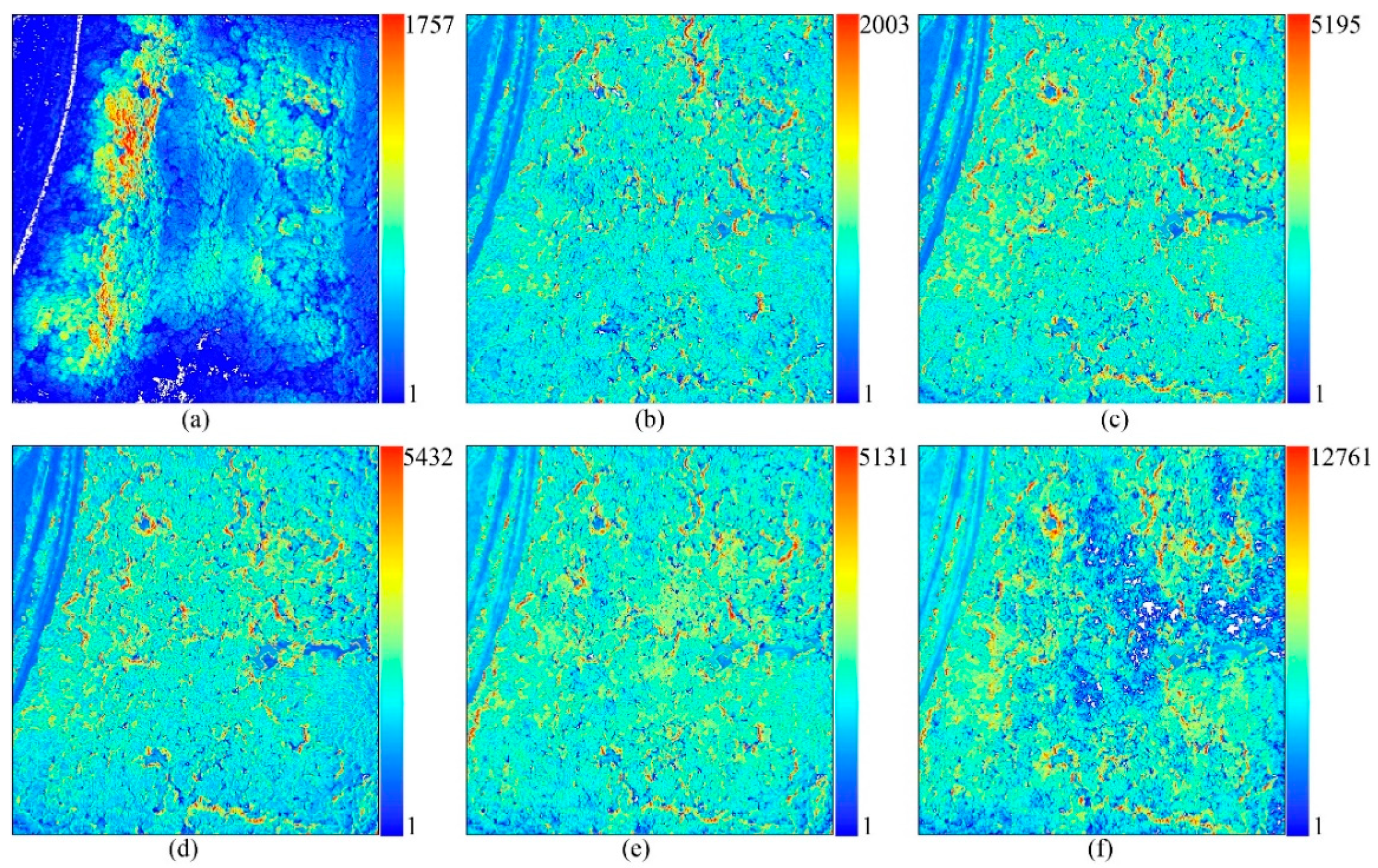
Table A2. The point cloud density of LiDAR data varied from 0 to 1757 points m
−2, with a mean of 168 points m
−2 in the grid at a 1.0 m resolution (
Figure A1).
The images were captured using a Canon EOS 5DS camera with a high-precision GNSS mounted on a six-rotor aircraft (see
Table 1 for detailed specifications) [
56,
57], and the lens had a focal length of 35 mm. The size of the image consisted of 8688 × 5792 pixels, which corresponds to the size of the sensor of 36.0 × 24.0 mm. The photogrammetry system was operated at different heights varying from 80 to 300 m (the ground sample distance (GSD) varied from 1 cm to 4 cm) with image overlaps varying from 64% to 84% to obtain five data sets (denoted as P1-D300, P2-D150, P3-D150, P4-D150 and P5-D80) covering the same area as shown in
Table A2. P1-D300 was acquired at a flying height of 300 m with a corresponding GSD of 4 cm. P2-D150, P3-D150 and P4-D150 were obtained at 150 m with a GSD of 2 cm using different across-track overlaps and flying speeds. P5-D80 was obtained at a flying height of 80 m with a corresponding GSD of 1 cm. The images were captured with an exposure time of 1/800 s or 1/1000 s on cloudy or sunny days using an automatic aperture and an ISO of 160. The images were processed to build a dense point cloud of the forest structure using the SfM method [
58]. Several steps were involved to generate high-precision dense point clouds. The images were aligned with high accuracy using the camera positions obtained by static differential processing of high-precision GNSS data. The camera and lens parameters, including the focal length, principal point coordinates, affinity and skew (non-orthogonality) transformation coefficients, radial distortion coefficients, and tangential distortion coefficients, were optimized to minimize the camera position errors using the optimize camera alignment tool [
58]. The dense points were built with high quality and mild depth filtering to maintain detailed characteristics of the forest canopies. The point cloud density of the photogrammetry data sets varied from 1 to 12,761 points m
−2, with means ranging from 257 to 2562 points m
−2 in the grid at a 1.0 m resolution (
Figure A1).
2.3. Data Processing
The LiDAR point cloud was classified as ground, vegetation, building, and noise using TerraSolid [
59]. The noise points were each carefully identified by visual evaluation. The ground algorithm was used to separate ground points from other objects with a maximum building size of 20 m, a terrain angle of 88°, an iteration angle of 6° to the plane and an iteration distance of 1.4 m to the plane. The ground points were modified by visual evaluation to eliminate false ground points. The points of artificial objects, such as water towers and buildings, were manually recognized. The remaining points were classified as vegetation after other objects were excluded. The L-DTM was generated from the ground points by a triangulated irregular network interpolation algorithm with spatial resolutions of 0.1, 0.2, 0.5, and 1.0 m [
9,
23,
35,
60,
61]. The original LiDAR DSM (L-DSM) was created from the vegetation and ground points by using maximum algorithms with spatial resolutions of 0.1, 0.2, 0.5, and 1.0 m [
9,
14,
28,
61]. The original LiDAR CHM (L-CHM) was produced based on the difference between the original L-DSM and L-DTM. The void cells of the original L-DSM were partially interpolated by the CN interpolation algorithm to generate the interpolated L-DSM. The interpolated L-CHM was produced based on the difference between the interpolated L-DSM and L-DTM.
The displacements between the LiDAR and photogrammetry point clouds were adjusted using the reference points extracted from the buildings and open ground area. The horizontal displacement was calculated based on roof ridges and building edges. The vertical displacement was computed according to the ground control points after horizontal displacement was applied. The aligned data sets were generated after the vertical displacement was applied. The photogrammetry dense point cloud was used to generate the original P-DSM by using the maximum algorithm. The interpolated P-DSM was created by the CN interpolation algorithm. The original P-CHM and the interpolated P-CHM were created from the corresponding P-DSMs normalized by the L-DTM [
23,
24,
25,
32,
33,
37,
48]. The DSMs and CHMs from LiDAR and photogrammetry were masked using the boundaries of the buildings and water towers to maintain consistency. The boundaries of the buildings were digitized according to the building points of the point cloud. Seventeen water towers with heights of approximately 38 m were distributed across the study site. The centres of the water towers were determined and used to create circular boundaries by buffering with a radius of 1.2 m.
2.4. Descriptors of Spatial Distribution
This study used three descriptors of the spatial distribution, namely, the ECR, PCH and PCR, to quantitatively depict the characteristics of the point cloud in the grid at the given spatial resolution. The original DSMs or CHMs obtained from LiDAR and photogrammetry may have void cells due to complex conditions, such as the laser scanning patterns, flight attitudes, and sunshine conditions [
14,
31,
51]. The ECR is defined as the proportion of effective cells to total cells (Equation (1)) and used to depict the distribution patterns of effective and void cells. The ECR reflects the uneven characteristics of point clouds to some degree. A small ECR means that many points are clustered in a small area.
where
is the effective cell ratio,
is the number of effective cells, and
is the number of total cells, including effective and void cells. If the
equals 1, then the point cloud is evenly distributed over each cell of the grid.
Different densities of points may occur in grid cells for different data sets with the same ECR. To explain the homogeneity of the point cloud distributed in the grid, the PCH is defined in Equation (2) by introducing the number of points per cell, which can be calculated as the product of the point cloud density per square metre and the cell area.
where
is the point cloud homogeneity,
is the mean number of points per cell by
,
is the number of total points, and
is the number of total cells. If
equals 1, then one point is located in each cell and the
is only determined by effective cells. If the
equals 1, then the
will be 1, regardless of how many points are located in each cell.
The PCR depicts the richness of points in each cell as defined in Equation (3). A lower PCH corresponds to a higher PCR, which indicates that some cells hold more unnecessary points. An evenly distributed data set should have a higher PCH and lower PCR.
where
is the point cloud redundancy,
is the effective cell ratio, and
is the mean number of points per cell. If the
and
both equal 1, then the points are ideally distributed evenly in each cell and the
equals 0. If the
is much greater than the
, then the
approximately approaches 1.
The ECR, PCH, and PCR of the point cloud could also be calculated based on the interpolated DSM or CHM. The interpolation introduced some degree of variation in these descriptors of the spatial distribution.
2.5. Constrained Neighbor Interpolation
The original DSM or CHM had void cells in the grid at a specified spatial resolution due to the uneven distribution of point clouds. The void cells can be filled using the effective neighboring cells. The number of effective neighboring cells (i.e., not including void neighboring cells) for one void cell varies from 1 to 8, which affects the spatial variation in the filled cells [
9,
14]. The CN interpolation algorithm is used to calculate the interpolated values for the void cells (Equation (4)).
where
(m) is the interpolated value of the
ith void cell,
(m) is the value of the
jth effective neighboring cell of the
ith void cell, k is the number of effective neighboring cells of the
ith void cell, and
Q is the threshold of effective neighboring cells of the void cell. The
ith void cell will be interpolated if the number of its effective neighboring cells is not less than the threshold (
Q).
The value of the threshold Q varies from 1 to 8. The void cell will be interpolated if there is at least one effective neighboring cells; that is, Q = 1. The ON interpolation algorithm will similarly interpolate the void cells with any effective neighboring cells, which can be regarded as the special case (Q = 1) of the CN interpolation algorithm. The CN and ON interpolation algorithms use an iterative process to interpolate the void cells. Some void cells with effective neighboring cells can be interpolated in the first loop, while other void cells may be interpolated in the second or more loops.
The void cells of different holes have a varied number of effective neighboring cells (
Figure 2). For example, the maximum number of effective neighboring cells of the void cells in
Figure 2a is 4, which will not be interpolated if the threshold
Q equals 5. Eight void cells will be interpolated in the first loop and 4 void cells interpolated in the second loop if the threshold
Q equals 4. In practice, any holes could be interpolated by iterative loops if the threshold
Q is less than 5. The runs of iterative loops will vary from several times to dozens of times depending on the number of void cells. The CN algorithm will continue to loop until every hole is either eliminated or reduced to a specific size as depicted in
Figure 2. The double width cross pattern of 12 cells would be the minimum hole if
Q equals 5 under normal circumstances in
Figure 2a. Another rarely occurring case would be that the interleaved chess pattern in
Figure 2e could not be interpolated. The small holes in
Figure 2b–d will not be interpolated if the threshold
Q equals 6, 7, or 8, while those holes can be filled if the threshold
Q equals 5. Therefore, the threshold of
Q = 5 is chosen for filling void cells in this study.
The hole in
Figure 2a is larger than the other holes in
Figure 2, and it is referred to as the diagnostic hole, which is used as the criteria to distinguish small and large holes. Small holes have one or more void cells, and the numbers of columns and rows of void cells were not less than 4. Large holes have twelve or more void cells, and both the numbers of columns and rows were equal to or greater than 4. The actual area of the diagnostic hole was determined based on the spatial resolution, for example, the area was 0.12 or 0.48 m
2 with a spatial resolution of 0.1 or 0.2 m, respectively.
2.6. Analysis of Spatial Resolution
The spatial resolution will affect the number of points in each cell of the original DSM or CHM. A fine spatial resolution tends to result in many void cells in the grid, while a coarse spatial resolution will discard many points in the effective cells of the grid for a given point cloud, which represents a compromise for determining the spatial resolution [
9,
14].
The spatial distribution characteristics of point clouds depend on the spatial resolution. The ECR will increase as the number of void cells decreases at a coarse spatial resolution. The interpolated void cells by the CN algorithm will also, to some degree, cause the ECR to increase. The variation in the ECR can be used to analyze the optimal spatial resolution for the DSM or CHM, in which as much information about the point cloud is retained as possible so that the void cells can be confidently interpolated in the grid. Series of ECR pairs of original DSMs and interpolated DSMs by the CN algorithm can be calculated at different spatial resolutions. The difference between the ECR of the interpolated DSM and that of the original DSM is referred to as the ECR pair difference, which is used as an indicator to select the spatial resolution. The ECR pair differences might decrease from fine to coarse spatial resolution when the void cells of the grid are interpolated by the CN algorithm. The optimal spatial resolution could be determined as the corresponding spatial resolution if the ECR pair differences do not become greater than the specified threshold (for example, 0.10). The series of spatial resolutions used as candidates is 0.1 m, 0.2 m, 0.5 m, and 1.0 m in this study. The optimal spatial resolution is considered relative to the other spatial resolution candidates.
2.7. Data Set Assessment
The estimated canopy heights obtained from the LiDAR data set were used as references to compare the estimated canopy heights obtained from five different photogrammetry data sets with spatial resolutions of 0.1, 0.2, 0.5, and 1.0 m. The overall mean difference (
) (Equation (5)) and mean absolute difference (
) (Equation (6)) were calculated for this purpose [
14,
23]. The canopy heights were divided into bins at 1.0 m intervals and used as a stratified variable to calculate a series of mean differences for analyzing the potential trends of canopy heights.
where
(m) is the overall mean difference,
(m) is the canopy height difference between LiDAR and photogrammetry for the
effective cell,
(m) and
(m) are the canopy heights of LiDAR and photogrammetry for the
effective cell (
), N is the total number of effective cells, and
(m) is the mean absolute difference.
The original and interpolated CHMs obtained from the LiDAR data set (response) were linearly regressed and analyzed with the corresponding CHMs of the five photogrammetry data sets (predictor). Three widely used statistical criteria, namely, the coefficient of determination (
) (7), root mean square error (
) (8), and relative
(
) (9), were used to assess the model accuracy [
41]. The
combines the mean error and error variance to provide a robust measure of overall accuracy [
62].
where
and
are the reference and estimated forest canopy heights (m) for the
ith effective cell (
), N is the total number of the reference canopy heights,
is the mean of the reference canopy heights,
is the mean error calculated by
,
is the
ith error and
is the error variance calculated by
.
3. Results
3.1. CHMs of LiDAR and Photogrammetry
The original L-DSM of the L-D55 data set with a spatial resolution of 0.1 m had many holes within and between crowns. The interpolation of the L-DSM by the CN algorithm filled all the small holes with areas less than 1.2 m
2. The hole-free L-DSM was generated by the ON algorithm. The original and interpolated L-CHMs were calculated based on the corresponding L-DSMs and L-DTM. The small holes of the original L-CHM with a spatial resolution of 0.1 m (
Figure 3a) were interpolated by the CN algorithm (
Figure 3b). All of the holes of the original L-CHM were filled by the ON algorithm except for the holes representing the water tower and building areas (
Figure 3c).
The P-DSMs of the five photogrammetry data sets were processed similarly to those of the LiDAR data set to generate original P-DSMs and those interpolated by the CN and ON algorithms, and the corresponding P-CHMs were generated by subtracting the L-DTM (
Figure 3d–l). The original P-CHM of the P1-D300 data set also had some small holes within crowns and large holes between the crowns, and the distributions of the holes were similar to the distribution of the holes in the L-CHM. The original P-CHMs of the P2-D150, P3-D150 and P4-D150 data sets had few small holes within crowns but large holes existed between the crowns. The original P-CHM of the P5-D80 data set had some large holes within the crowns and much larger holes between the crowns than any other data set. The large holes were mainly distributed in the shadow area of tree crowns.
3.2. Spatial Distribution of Point Clouds
The spatial distribution of the point clouds was described using the ECR, PCH and PCR. The calculated ECRs, PCHs and PCRs of the original and interpolated L-CHMs with spatial resolutions of 0.1, 0.2, 0.5, and 1.0 m were shown in
Figure 4. The ECRs of the original and interpolated L-CHMs increased as the spatial resolution changed from 0.1 to 1.0 m. The ECRs of the original L-CHM with a spatial resolution of 1.0 m were still less than 1.0, which indicated that some areas had sparsely distributed points due to weak ability of backscattering. The CHMs interpolated by the ON algorithm achieved the ideal ECR of 1.0 for any spatial resolution, although the method introduced great spatial variations and decreased the accuracy of the estimated canopy heights.
The ECRs, PCHs and PCRs of P-CHMs are shown in
Figure 4. All the ECRs of the original P-CHMs were greater than those of the L-CHM at spatial resolutions less than 1.0 m, which indicated that the photogrammetry data sets had fewer holes than the LiDAR data set. The ECRs of the original and interpolated P-CHMs also increased as the spatial resolution decreased.
The PCH of the original L-CHM was less than that of the original P-CHMs of most photogrammetry data sets except for P-D80 with a spatial resolution of 0.1 m, which showed that the dense point cloud of photogrammetry was more evenly distributed than the LiDAR point cloud. The low PCH of the original P-CHM of the P-D80 data set was caused by many large holes due to the failed reconstruction of the dense point cloud. The PCHs of the original L- and P-CHMs decreased continuously as the spatial resolution decreased. The PCRs of the original P-CHMs were all higher than those of the L-CHM, indicating that there were more redundant points in the photogrammetry data sets.
The difference between the ECRs of the original L-CHM and interpolated L-CHM by CN at the spatial resolution of 0.1 m was the largest (0.19) compared with those at other spatial resolutions. The ECR pair differences decreased as the spatial resolution decreased. The optimal spatial resolution of L-CHM was 0.2 m if the threshold of the ECR pair difference was set as 0.10. The optimal spatial resolution of P-CHMs was 0.1 m when the same threshold of the ECR pair difference as that of L-CHM was used.
3.3. Differences between L-CHMs and P-CHMs
The differences between the original and interpolated L- and P-CHMs were calculated on a cell-by-cell basis. The void cells of the holes might not have corresponding cells among different CHMs. These cells were ignored if there was a void cell in either of the CHM pairs used to calculate the differences. The mean differences between the original L-CHM and original P-CHMs with a spatial resolution of 0.1 m varied from −0.1 to −0.5 m, while the corresponding mean absolute differences varied from 0.9 to 1.1 m (
Table A3). This result indicated that the original L-CHM was lower overall than the original P-CHMs and large positive and negative differences occurred within the original CHMs of different data sets. The mean differences between the original L-CHM and P-CHMs increased from negative to positive as the spatial resolution became coarser because low values within cells were ignored when CHMs with a coarse spatial resolution were generated using the maximum algorithm. The mean absolute differences between the original L-CHM and original P-CHMs decreased as the spatial resolution increased, which indicated that the spatial variation in canopy heights was suppressed at a coarse spatial resolution.
The mean differences and mean absolute differences between the LiDAR and photogrammetry data sets slightly increased when the CHMs were interpolated by the CN algorithm compared with the original CHMs. The mean differences and mean absolute differences further increased using the CHMs that were interpolated by the ON algorithm compared with the CHMs interpolated by the CN algorithm.
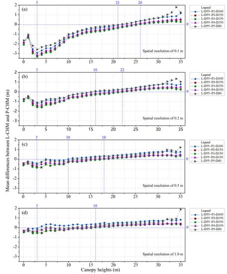
The stratified mean differences between the original L-CHM and P-CHMs within the 1.0 m bin of the canopy heights were calculated to analyze the spatial variations among canopy heights (
Figure 5). Three mark heights of mean differences were observed along the canopy heights, including the minimum mark height, negative mark height and positive mark height. The minimum mark height of the mean difference between CHMs at a spatial resolution of 0.1 m was the 3.0 m bin of the canopy height corresponding to a minimum mean difference of 3.3 m. All the mean differences between CHMs with a spatial resolution of 0.1 m were negative when the canopy height was less than the 21.0 m bin and were positive when the canopy height was greater than the 26.0 m bin, which were referred to as negative and positive mark heights, respectively. The mean differences increased from negative to positive as the canopy height increased above the 3.0 m bin. This result indicated that photogrammetry tends to overestimate the low canopy heights and underestimate the high canopy heights compared to those obtained from LiDAR data.
The minimum mean differences increased from −3.3 to −0.6 m as the spatial resolution changed from 0.1 to 1.0 m. The negative and positive mark heights both shifted from high bins to low bins as the spatial resolution became coarser.
3.4. Correlation between L-CHMs and P-CHMs
The original and interpolated L-CHMs (responses) were regressed with the corresponding original and interpolated P-CHMs (predictors) (see
Figure 6). High correlations were observed between the LiDAR and photogrammetry data sets at different spatial resolutions as shown by the
, which varied from 0.87 to 0.98. The original L-CHMs were better correlated with P-CHMs at a coarse spatial resolution than a fine spatial resolution. The
between the original L-CHMs and P-CHMs decreased as the spatial resolution changed from 0.1 to 1.0 m.
The L-CHMs and P-CHMs interpolated by the CN algorithm had slight effects on the and root mean square errors (RMSEs) compared with those between the original L-CHM and P-CHMs. The RMSEs between the interpolated L-CHM and P-CHMs by the ON algorithm were higher than those between the interpolated CHMs by the CN algorithm, which was expected. The relative RMSEs between the interpolated L-CHM and P-CHMs by the ON algorithm increased by approximately 3.1% compared with those between the original L-CHM and P-CHMs with a spatial resolution of 0.1 m. This result indicated that the ON interpolation algorithm would introduce obvious spatial variation into the CHM at fine spatial resolution. The relative RMSE decreased as the spatial resolution became coarser.
4. Discussion
4.1. Spatial Distribution of Point Clouds
The spatial distribution of point clouds is usually uneven across a survey area due to various conditions, such as the LiDAR or photogrammetry system configuration, flying height, crown shadows, or terrain conditions [
43,
44,
45,
63]. At different locations, some points are closely clustered while other points are sparsely distributed. The mean point density can describe only the overall characteristics of point clouds and does not reflect the features of uneven distributions. The ECR, PCH and PCR are used to describe the spatial distribution of point clouds based on regular grids.
The spatial resolution determines the number of points located within each cell of the grid and affects the values of these spatial descriptors. The coverage, homogeneity and redundancy of point clouds are dependent on the spatial resolution of the grid. The coverage of the point clouds will increase at a coarse spatial resolution if the ECR is less than 1.0, the homogeneity of the point clouds will decrease at a coarse spatial resolution, while the redundancy of the point clouds will increase at a coarse spatial resolution.
The relative correlation of the spatial distribution of different data sets might remain constant. For example, P3-D150 had the best coverage, L-D55 had the worst coverage, P1-D300 was the most evenly distributed data set, P5-D80 had the worst homogeneity, L-D55 had the lowest redundancy, and P5-D80 had the most redundant points, and these observations were all based on CHMs with the same spatial resolution (
Figure 4). The ideal data set should have the maximum coverage, best homogeneity and lowest redundancy. No data set fulfilled these criteria in this study case.
4.2. Effects of the CN and ON Algorithms on the CHM
The void cells of the CHM could be filled by a neighbor interpolation algorithm. The ON algorithm continuously interpolates void cells from the outside cells to inside cells. On the other hand, the CN algorithm interpolates only void cells that meet the criteria of neighboring cells. For example, if the threshold of effective neighboring cells (Q) is 5, the void cells along the edges of a large hole will not be filled while the void cells at the corners will be conditionally filled by the CN algorithm.
The interpolated void cells of the CHM by the CN algorithm varied as the spatial resolution changed and produced different ECR values (
Figure 4). The ON algorithm interpolated all void cells and obtained the same ECR at all spatial resolutions. If the dimension of the spatial resolution was much smaller than the distance of the point cloud, then the number of the effective neighboring cells of void cells was smaller than the threshold of effective neighboring cells (
Q) and no void cells were interpolated by the CN algorithm. If the dimension of the spatial resolution was larger than the size of the maximum hole, then the ECR was equal to 1.0. The CN algorithm had no effect on the ECR of the CHM according to these two mentioned cases.
The CN algorithm had a weak effect on the mean absolute differences between the L-CHM and P-CHMs at the spatial resolution of 0.1 m. The mean absolute differences between the original L-CHM and original P-CHMs at the spatial resolution of 0.1 increased by 0.2 m compared with that between the L-CHM and P-CHMs interpolated by the ON algorithm (
Table A3). The effects of the CN and ON algorithms on the mean absolute differences both became weaker at a coarser spatial resolution.
The relative RMSEs between the L-CHMs and P-CHMs interpolated by the ON algorithm were larger than those between the CHMs interpolated by the CN algorithm at all spatial resolutions. The CN algorithm had the ability to control the spatial variation introduced by the ON algorithm. Thus, the CN algorithm is recommended for interpolating the void cells of a CHM rather than the ON algorithm.
4.3. Distinguishing Small and Large Holes within a CHM
The holes within a CHM with a specified spatial resolution consist of one or several continuous void cells. Small holes in an L-CHM are usually caused by the fluctuation of the UAV platform, mutual obscuration of crowns, gaps within and between crowns, lost echoes of laser pulses, etc. Large holes in an L-CHM are mainly affected by the large incident angles on crowns and the loss of many backscattering signals. The influencing factors of small and large holes of the P-CHM include the reconstruction algorithm of dense point clouds, the quality of images, illumination conditions, texture of crowns, pits of crowns, gap between crowns, and swinging of crowns due to wind. Large holes in the P-CHM are mostly due to weak texture and poor lighting (extremely bright or dim). The light conditions of different photogrammetry data sets are very different and will cause different shadows to affect the spatial distribution of the reconstructed point cloud.
The coverage of holes is the ratio of void cells to all cells expressed as 1-ECR. The original CHM with a fine spatial resolution might include small and large holes, while the CHM interpolated by the CN algorithm would include only large holes. For example, the area covered by holes of the original L-CHM with a spatial resolution of 0.1 m was 38% of the whole area. The large holes (≥0.12 m2) of the interpolated L-CHM occupied 19% of the whole area. This result indicated that 50% of the holes were large holes. The percent of large holes (≥0.48 m2) decreased to 40% of the holes when the spatial resolution of the original L-CHM was 0.2 m. The minimum size of large holes further increased, and the percent of large holes further decreased when the spatial resolution of the L-CHM became coarser.
4.4. Optimal Spatial Resolution of the CHM
The spatial resolution of a CHM is usually determined by considering the mean point cloud density. Many void cells will exist within the CHM at this spatial resolution if the point cloud is unevenly distributed across the survey area. Small holes of the CHM can be interpolated by the CN algorithm. The interpolated cells reflect the potential space that would become effective cells at a coarse spatial resolution. The optimal spatial resolution may be determined by the potential space, which is referred to as the potential space criteria. The potential space is calculated as the difference between the ECRs of the original CHM and the CHM interpolated by the CN algorithm.
The optimal spatial resolution can also be determined by the ECR of the CHM interpolated by the CN algorithm, which is referred to as the ECR criteria. If the ECR approaches 1 and is greater than the specified threshold (for example, 0.90), then the corresponding spatial resolution will be regarded as optimal. The ECR criteria are easily affected by very large holes, whose sizes are far greater than the mean space of the point cloud. Additional criteria can be used to select the optimal spatial resolution. We recommend potential space criteria that will not be affected by large holes. Moreover, the optimal spatial resolution can be simply determined by the ECR pair differences among predefined spatial resolutions, which should be calculated by automatic methods in future studies.
4.5. Effects of Flying Configuration on the CHM
Five photogrammetry data sets at three different flying heights were used in this study. P1-D300 had the highest flying height and a highly efficient capability of data acquisition when compared to the other data sets collected at lower flying heights. The optimal spatial resolution of P1-D300 was 0.1 m if the threshold of the difference between the ECRs of the original CHM and the CHM interpolated by the CN algorithm was 0.1. Therefore, an optimal flying height of approximately 300 m was recommended to generate a CHM at a spatial resolution of 0.1 m using the similar photogrammetry system in this study.
The P5-D80 data set had the lowest flying height among the photogrammetry data sets, although the ECRs of the original P-CHM of P5-D80 were smaller than those of the other photogrammetry data sets. Very large holes exist within the bright crown area in the original P-CHM of the P5-D80 data set. This finding indicated that some tree crowns failed to be reconstructed using images with very high spatial resolution.
Different shadows occurred in the photogrammetry data sets with different light conditions, and these differences would affect the distribution patterns of void cells in the P-CHMs. The overall effects of light conditions on the reconstructed point cloud and the P-CHMs were weaker than the effects of the flying height in this study. The ECRs of the original P-CHMs with a spatial resolution of 0.1 m had slight differences under different light conditions at the same flying height of 150 m. The differences among the ECRs of the P-CHMs with a spatial resolution of 0.1 m at flying heights of 80, 150 and 300 m were greater than those among the ECRs of the P-CHMs at the same flying height of 150 m.
The mean differences between the combined pairs of photogrammetry data sets were smaller and fluctuated from −0.5 m to 0.5 m when the canopy heights were less than 30 m. Obviously large variations occurred when the canopy heights were greater than 30 m. This variation might be due to the swinging of leaves and twigs of tall trees affected by wind. The mean differences between the combined pairs of the P2-D150, P3-D150 and P4-D150 data sets at the same flying heights were smaller than those of other pairs at different flying heights for all canopy height bins.
The mean differences between the P2-D150 and P4-D150 data sets with different image overlaps varied from 0 m to 0.1 m, which meant that image overlap (>68%) had a minor effect on the estimated canopy height. However, the point density of the photogrammetry data set was substantially affected by image overlap (
Figure A1). The mean differences between the P2-D150 and P3-D150 data sets with different flying speeds varied from −0.2 to 0 m, indicating that canopy height was only slightly affected by flying speed (<8 m s
−1).
4.6. Effects of Gaps within and between Crowns on the CHM
The CHMs obtained from LiDAR and photogrammetry data sets for the given spatial resolution were affected by the gaps within and between crowns [
14,
23,
27]. Small gaps within crowns could be depicted in the L-CHM with fine spatial resolution, while the P-CHM tended to ignore such small gaps [
23]. A number of deep gaps were observed between the tall tree crowns, which were much darker than the surrounding crowns under the variable illumination conditions. It was difficult to reconstruct the spatial structure in these deep gaps [
14,
38].
The spatial resolution will affect the height values of gaps within and between crowns. The cells of a CHM are often calculated as the highest value if there are numerous points within the corresponding cell. This condition will suppress the low values of gaps and promote high values of crowns, thus reducing the spatial variation in the canopy heights. LiDAR can provide more detailed structural information than photogrammetry on a fine scale and more details will be lost on a coarse scale. The CHMs between LiDAR and photogrammetry tend to have more consistency as the spatial resolution decreases.
5. Conclusions
This study compared the canopy heights obtained from UAV LiDAR and UAV photogrammetry and interpolated by two spatial interpolation algorithms CN and ON. The comparison was conducted based on three proposed spatial distribution descriptors of point clouds: the ECR, PCH and PCR quantifying the unevenness, homogeneity and redundancy characteristics, respectively, of point clouds in the grid at a given spatial resolution. The stratified mean differences revealed that there existed an inherent trend between the estimated canopy heights from LiDAR and photogrammetry, which changed from negative to positive as the canopy heights increased. The LiDAR CHM strongly correlated with the photogrammetry CHM. More importantly, the CN algorithm had the ability to distinguish small and large holes and determine the optimal spatial resolution according to the ECR pair differences, while the ON algorithm did not have this ability. Compared with the ON algorithm, the CN algorithm apparently reduced the spatial variation in the CHM, led to smaller RMSE values, and could be recommended to obtain reliable CHM values.
Some large holes in the CHMs interpolated by the CN interpolation algorithm still occurred at very high point densities, which were typically distributed around the deep gaps between tall tree crowns. Precisely measuring such deep gaps is quite challenging. Photogrammetry tends to ignore gaps within the crowns, overestimate low canopy heights and underestimate high canopy heights; these issues need to be considered while canopy cover, canopy closure, and forest stand height are modelled. Overall, this article provides an operational method for the spatial assessment of point clouds and suggests that the differences between LiDAR and photogrammetry derived CHMs should be considered when forest parameters are estimated. In particular, further study is necessary to enhance understanding the quality measures of the point cloud spatial distribution, optimal spatial resolution, small and large holes within CHMs, gaps within and between crowns, and their effects on estimation of forest parameters using additional data sets.

 ,
, 


