Article

Prediction of Individual Tree Diameter and Height to Crown Base Using Nonlinear Simultaneous Regression and Airborne LiDAR Data

1
Research Institute of Forest Resource Information Techniques, Chinese Academy of Forestry, Beijing 100091, China
2
Key Laboratory of Forest Management and Growth Modeling, National Forestry and Grassland Administration, Beijing 100091, China
3
College of Information Science and Technology, Nanjing Forestry University, Nanjing 210037, China
4
College of Mathematics and Statistics, Xinyang Normal University, Xinyang 464000, China
5
Institute of Forestry, Tribhuwan Univeristy, Kritipur, Kathmandu-44600, Nepal
6
Department of Geography and Environmental Resources, Southern Illinois University at Carbondale, Carbondale, IL 62901, USA
*
Author to whom correspondence should be addressed.
These authors contributed equally to this work.
Remote Sens. 2020, 12(14), 2238; https://doi.org/10.3390/rs12142238
Submission received: 18 June 2020 / Revised: 28 June 2020 / Accepted: 29 June 2020 / Published: 13 July 2020
(This article belongs to the Special Issue Advances in Remote Sensing for Global Forest Monitoring)

Abstract

:
The forest growth and yield models, which are used as important decision-support tools in forest management, are commonly based on the individual tree characteristics, such as diameter at breast height (DBH), crown ratio, and height to crown base (HCB). Taking direct measurements for DBH and HCB through the ground-based methods is cumbersome and costly. The indirect method of getting such information is possible from remote sensing databases, which can be used to build DBH and HCB prediction models. The DBH and HCB of the same trees are significantly correlated, and so their inherent correlations need to be appropriately accounted for in the DBH and HCB models. However, all the existing DBH and HCB models, including models based on light detection and ranging (LiDAR) have ignored such correlations and thus failed to account for the compatibility of DBH and HCB estimates, in addition to disregarding measurement errors. To address these problems, we developed a compatible simultaneous equation system of DBH and HCB error-in-variable (EIV) models using LiDAR-derived data and ground-measurements for 510 Picea crassifolia Kom trees in northwest China. Four versatile algorithms, such as nonlinear seemingly unrelated regression (NSUR), two-stage least square (2SLS) regression, three-stage least square (3SLS) regression, and full information maximum likelihood (FIML) were evaluated for their estimating efficiencies and precisions for a simultaneous equation system of DBH and HCB EIV models. In addition, two other model structures, namely, nonlinear least squares with HCB estimation not based on the DBH (NLS and NBD) and nonlinear least squares with HCB estimation based on the DBH (NLS and BD) were also developed, and their fitting precisions with a simultaneous equation system compared. The leave-one-out cross-validation method was applied to evaluate all estimating algorithms and their resulting models. We found that only the simultaneous equation system could illustrate the effect of errors associated with the regressors on the response variables (DBH and HCB) and guaranteed the compatibility between the DBH and HCB models at an individual level. In addition, such an established system also effectively accounted for the inherent correlations between DBH with HCB. However, both the NLS and BD model and the NLS and NBD model did not show these properties. The precision of a simultaneous equation system developed using NSUR appeared the best among all the evaluated algorithms. Our equation system does not require the stand-level information as input, but it does require the information of tree height, crown width, and crown projection area, all of which can be readily derived from LiDAR imagery using the delineation algorithms and ground-based DBH measurements. Our results indicate that NSUR is a more reliable and quicker algorithm for developing DBH and HCB models using large scale LiDAR-based datasets. The novelty of this study is that the compatibility problem of the DBH model and the HCB EIV model was properly addressed, and the potential algorithms were compared to choose the most suitable one (NSUR). The presented method and algorithm will be useful for establishing similar compatible equation systems of tree DBH and HCB EIV models for other tree species.

Graphical Abstract

1. Introduction

A tree crown is characterized by crown height, crown width, crown density, leaf area, and crown ratio, and their measurements are useful for forest management and research. The crown ratio is considered a reliable indicator of the vigor and potential growth of a tree [1,2,3,4]. Height to crown base (HCB) is an important tree measure to derive crown ratio and is also regarded as an indicator of log quality. HCB is usually understood as the vertical height from the ground to the bottom of live whorled branch on the bole of a tree [5]. The ground-based measurement of HCB is a time-consuming and labor-intensive process; thus, it is rarely done during field inventory [6,7]. Most researchers have obtained the HCB value by establishing linear or nonlinear HCB models with other variables as predictors, such as DBH, tree height, basal area, basal area larger than a target tree, the sum of basal area of all trees with diameter bigger than a target tree, crown competition factor, climate, and site index [8,9,10,11,12]. Tree diameter at breast height (DBH) is also an important tree attribute that is used as a main predictor in forest growth and yield, taper, and biomass models. In general, the measurement of DBH is very common in ground-based inventory; however, field-inventory data could have a low accuracy, and their measurement needs more time and cost, especially measurements required for extensive forest areas. Therefore, methods of HCB data collection have been transformed from the traditional forest field inventory to modeling and prediction based on remote sensing technology [13,14,15,16].
Light detection and ranging (LiDAR) can accurately determine the geographical position of surface objects by transmitting and receiving laser pulses. Laser pulses travel down the forest canopy, and detailed information on the three-dimensional structures of the forest canopy and understory topography can be obtained [17]. Many tree attributes, such as tree height and crown dimensions [18] can be obtained based on the LiDAR data. The study approaches based on HCB prediction may be divided into two categories: direct and indirect approaches. The direct approaches refer to those derived from HCB with various geometrical shapes of the crown [12,19,20,21,22,23] or predicting HCB according to descriptive statistics of the LiDAR-based data distribution [4,24]. Direct approaches do not require any ground-measured HCB data, which are costly and time-consuming, as they only require point-cloud data processing and analysis including tree detection and the determination of crown base positions. In addition, this approach could also cause considerable uncertainties in determining the base of the first normal green branch as a part of the crown. Therefore, its application is quite limited to estimating HCB. The indirect approach, on the other hand, refers to predicting HCB through the application of statistical modeling [22,25,26,27,28]. This approach requires field-measured HCB data to establish the models for the prediction of HCB. The models for the accurate prediction of individual tree HCB can be built using LiDAR-based information, and so this method has been frequently used in recent years [22,25,26,27,28].
The application of ordinary least square (OLS) regression to estimate the parameters of LiDAR-based DBH and HCB models is not generally preferred, but it is still used [16,29]. This estimation method usually assumes that (i) regressors are random variables with errors, (ii) regressors are fixed variables without errors, and (iii) the associated error is subject to normal distribution with zero mean and constant variance [30]. Any violation of the second assumption leads to the substantially biased estimation of the models [30], which eventually reduces the prediction accuracy.
The prediction accuracy of the developed HCB and DBH models uses the LiDAR-based tree height, crown width and crown area may not be always satisfactory for a couple reasons. Firstly, LiDAR-based tree height, crown width, and crown area have random or systematic errors caused by LiDAR system configuration and parameter estimation. Any error involved in the variables could increase the residual variance of the model and also lead to invalid statistical tests [31,32]. Secondly, the estimated DBH from a LiDAR-based DBH estimation model contains non-ignorable or inevitable errors [33]. If such erroneous DBH is used as a predictor in a LiDAR-based HCB model, substantial bias would occur due to error transfers [34]. In addition, estimating with a LiDAR-based DBH model and a LiDAR-based HCB model separately or independently using OLS disregards the inherent correlations of HCB with DBH and thus fails to account for the compatibility of the estimated HCB and DBH. Thus, estimating the parameters of both model types independently with OLS may create a remarkable problem, especially in the condition when errors are associated with both the regressors and response variables. An appropriate settlement of this problem is to apply error-in-variable (EIV) modeling, which takes the errors into consideration and can guarantee compatibility between HCB and DBH [29,35,36,37].
Fuller [35] first introduced the theory on the development and application of linear EIV models, and, later on, Carroll et al. [32] applied this concept on the nonlinear EIV modeling in detail. Kangas [31] investigated the effects of EIV on the parameters of the diameter growth model and applied the simulation extrapolation algorithm to adjust the errors in the estimated parameters. Lindely [38] proved that validation data from the same population as the fitting data resulted in predictions that were usually unbiased, even though the regressors were subject to error. Tang and Zhang [36] developed an EIV model to investigate the unbiased parameter estimates. Tang and Wang [39] proposed the two-stage EIV method to estimate the model parameters. In their study, the EIV concept was introduced into forest attribute modeling, which provides a theoretical basis for studying the influence of errors on stand growth and harvest models. Li and Tang [40] compared three methods, namely simulation extrapolation, regression calibration, and EIV to estimate the models and found a better performance with EIV with smaller variances compared to other two methods.
Few studies have been carried out with DBH EIV modeling using remote sensing data. For example, Fu et al. [33] developed an individual tree DBH and above-ground biomass (AGB) EIV model with LiDAR-based tree height and crown projection area as predictors with the application of the two-stage error-in-variable modeling (TSEM) and nonlinear seemingly-unrelated regression (NSUR) to estimate model parameters. Both TSEM and NSUR explain the correlations of DBH with AGB and also effectively explain the errors in DBH on the prediction of AGB. Zhang et al. [29] reported that the DBH EIV model developed with errors associated with both response and regressor variables through the application of the maximum likelihood method was most appropriate. To the authors’ knowledge, no studies have been carried out on developing LiDAR-based HCB EIV models that were attributed to compatibility.
This study thus aimed (a) to develop a compatible simultaneous equation system of DBH and HCB EIV models based on the LiDAR data at the individual tree level for Picea crassifolia Kom forests in northwest China, (b) to evaluate the compatibility of two different nonlinear OLS-based DBH and HCB models with the leave-one-out cross validation method, and (c) to compare various unbiased fitting algorithms including NSUR. To simplify the proposed simultaneous equation system and to guarantee its application in the future, only response variables (HCB and DBH) were assumed as the error-in-variables [39], and predictor variables were regarded as error-out variables [33]. The presented compatible simultaneous equation system of DBH and HCB models will be applicable to other Picea species whose growth and stand conditions are very much similar to the basis of our studied species. This tree species is crucial to the economic and social development of the rural population, as well as regional carbon storage and cycling, and the maintenance of the structures and functions of the forest ecosystems in northwest China. This article is mainly concerned with the methodology employed in this study, which is clearly described in the Methods section; additionally, the major strengths and weaknesses of the methodologies, along with the main findings of the study, are thoroughly discussed while the potential contribution of the study is highlighted.

2. Methods

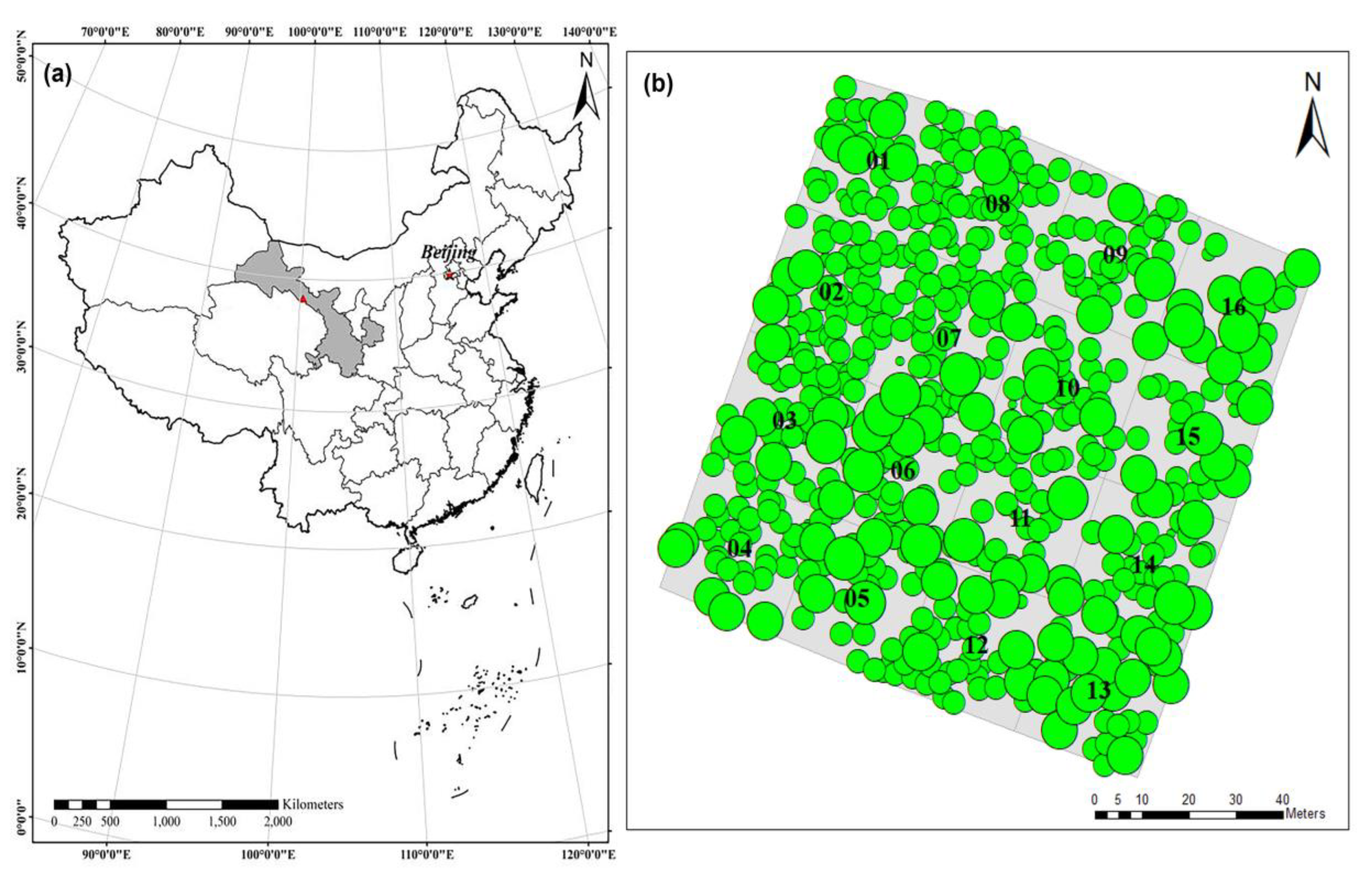
2.1. Data Collection

The study site is located at the Xishui forest farm of the Su’nan Yuguzu autonomous county, Gansu province (38°29′–38°35′N, 100°12′–100°20′E) (Figure 1a) with Picea crassifolia Kom as the dominate tree species. The climate in this field is a temperate semi-arid zone. It is covered by mountainous forests. Slopes with south-facing aspect are covered by grass, and the slopes with north-facing aspect are covered by natural secondary pure forests with one dominating tree species of Picea crassifolia Kom. The ground is covered by a moss floor, and the average elevation here is around 2993 m. The typical soil type is sandy loam. Along the hill, we established a permanent sample plot (PSP) with 100 m long and 100 m wide in 2008, and the PSP was divided into sixteen sub-plots that were 25 m long and 25 m wide. The PSP designed in this study was very representative of the entire forest of the study area and was mainly used for the carbon flux observation and dynamic monitoring of forest quality.
Airborne LiDAR data were acquired by the LiteMapper 5600 system with laser scanner—Riegl LMS-Q560 by a specification of 50 kH pulse repetition frequency, a 49 HZ scanning frequency, and a 30° maximum scanning angle [41]. The LiDAR data were collected on 23 June 2008, and field-measured data were collected on 1 June through 13 June 2008. The wavelength was 1550 nm, and the pulse length and laser beam divergence were 3.5 ns and 0.5 mrad, respectively. The average flight height was 3699 m, and the average flight speed was 230 km h−1. The scanner’s pulse repetition frequency, scanning frequency, and maximum scanning angle were 50 kHZ, 49 Hz, and 30°, respectively, and the mean density of point cloud was 4.34 m−2. The spatial distribution of neighbor smoothed 510 Picea crassifolia Kom trees is shown in Figure 1b. Data summary is presented in Table 1, and the relationships of HCB with DBH, LiDAR-derived tree height (LH), LiDAR-derived crown width (LCW), and LiDAR-derived crown projection area (LCA) are shown in Figure 2.
The correlation analysis of LiDAR-derived tree attributes and ground-measured tree attributes are shown in Figure 3, which indicates that these LiDAR-derived tree attributes are highly correlated with ground-measure tree attributes. Thus, these LiDAR-derived tree attributes in the sample could be used for our modeling study. Figure 4 presents the Y coordinate value versus the predicted HCB value showing the vertical profile of the LiDAR product.
The point cloud was created from LiDAR waveforms by the data provider [41]. By applying the algorithm of TerraScan 005 (Terrasolid, Helsinki, Finland), the ground points were classified, and this was used to create the digital elevation model (DEM) (Figure 5a) with a 0.25 m resolution. With ground and vegetation points, the digital surface model (DSM) with a 0.25 m resolution was created using the Highest hit z algorithm of TerraScan 005. A canopy height model (CHM) (Figure 5b) with a resolution of 0.25 m and a window size of 3 × 3 m was obtained by subtracting the DSM and DEM [42,43,44]. The pits in the CHM were smoothed by neighbor smoothing algorithm [45]. Using the local maximum method with a window size of 2.0 m to detect the crown top from the CHM, the LH values were estimated as the values of detected crown tops with a prediction accuracy of 0.65. Using the region growing algorithm proposed by Liu et al. [46], the LCW of each tree was estimated to be the average of the horizontal ranges of the identified crown from west to east and north to south [45]. After determining canopy boundary, the LCA was obtained. Ground measurements were done for various tree attributes including individual tree DBH, HCB, crown width, and total tree height (H) of 16 sub-plots for a total of 510 Picea crassifolia Kom trees.

2.2. Base Model

2.2.1. LiDAR–DBH Base Model

Fu et al. [33] developed an exponential LiDAR-based DBH model using LH and LCA as predictors for Picea crassifolia Kom and found a significantly higher prediction accuracy than other three candidate LiDAR-based DBH model forms (linear, Richards, and logistic). Our preliminary analyses exhibited the biggest R 2 and the smallest root mean square error (RMSE) of the exponential LiDAR-based DBH model form, indicating its greatest suitability according to our data characteristics, and its prediction accuracy could be further improved by including LH and LCW as predictors (Equation (1)):
D B H = β 1 exp ( β 2 L H β 3 L C W ) + ε D B H
where β 1 , β 2 , β 3 are parameters to be estimated, and ε D B H is a residual error.

2.2.2. LiDAR–HCB Base Model

Similar to Walters and Hann [40], we used the logistic model as a LiDAR–HCB base model, which had DBH and LCA as predictors in this study.
H C B = L H 1 + exp ( γ 1 D B H + γ 2 L C A ) + ε H C B
where γ 1 and γ 2 are parameters to be estimated, and ε H C B is a residual error.

2.3. A Compatible Individual Tree DBH and HCB EIV Equation System

A compatible equation system consisting of tree-based DBH and HCB EIV models (Equation (3)) was built by integrating both the LiDAR–DBH base model (Equation (1)) and the LiDAR–HCB base model (Equation (2)) by following the methods suggested by existing modeling studies [36,37,47].
{ d b h i = β 1 exp ( β 2 L H i β 3 L C W i ) h c b i = L H i / ( 1 + exp ( γ 1 D B H i + γ 2 L C A i ) D B H i = d b h i + ε D B H i H C B i = h c b i + ε D B H i ε i = ε D B H i + ε H C B i
where D B H i (cm) and H C B i (m) ( i = 1 , 2 , N ) are the ground-measured diameter at breast height with errors and height to crown base with errors of the ith tree, respectively; d b h i and h c b i are true values (with the assumption of no errors) of D B H i and H C B i , respectively; ε D B H i and ε H C B i represent the errors of D B H i and H C B i , respectively. Error ε i is a two-dimensional vector that is assumed to be normally distributed with zero means and variance–covariance matrix Σ ; L H i , L C W i , and L C A i are the LiDAR-derived tree height (m), crown width (m), and crown projection area (m2) of the ith tree, respectively. In this simultaneous equation system (Equation (3)), both DBH and HCB are the EIV, while LH, LCW, and LCA are regarded as error-free variables. The other parameters and variables are the same as defined above. The elements in the variance–covariance matrix Σ were applied to account for the inherent correlations of DBH with HCB.
It was assumed that the simultaneous equation system (Equation (3)) with an error term ε t i (t = DBH and HCB; and i = 1,…, N) that were not correlated among the observations but were contemporaneously correlated across the sub-models. For each observation, we assumed that:
Σ = ( σ D B H × D B H σ D B H × H C B σ H C B × D B H σ H C B × H C B )
where σ D B H × D B H , σ H C B × H C B , σ D B H × H C B , and σ H C B × D B H are the variance and covariance related elements for both DBH and HCB.
The covariance matrix of the stacked error terms ( ε = ( ε D B H T , ε H C B T ) T ( ε t = ( ε t 1 , , ε t N ) T , t = D B H   a n d   H C B ) would be R   =   Σ I N .

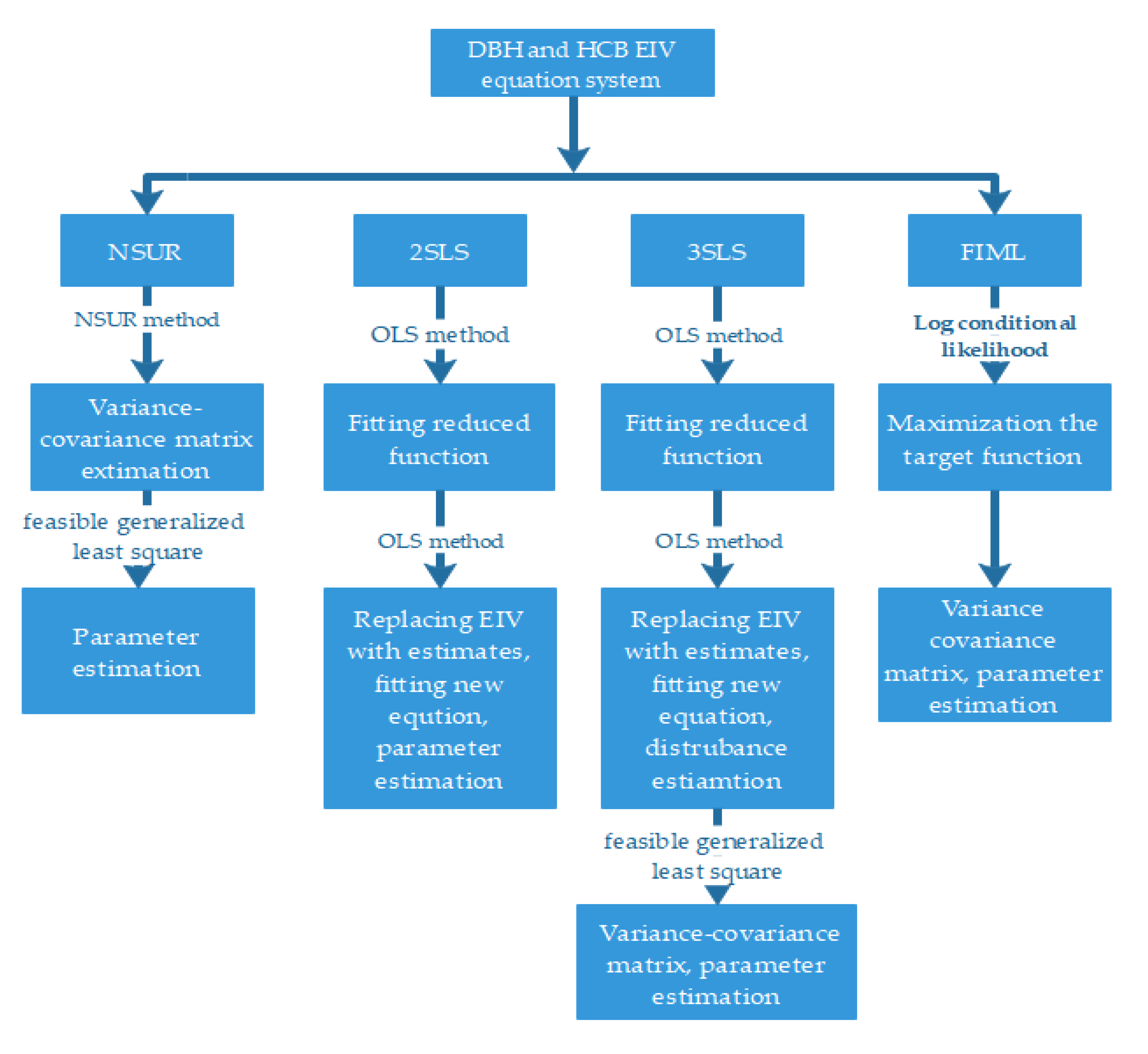
2.4. Parameter Estimation

Four commonly used algorithms, such as NSUR, two-stage least square (2SLS), three-stage least square (3SLS), and full information maximum likelihood (FIML) were applied to estimate the parameters B   =   ( β DBH T   =   ( β 1 , β 2 , β 3 ) , γ H C B T   =   ( γ 1 , γ 2 ) ) in our simultaneous equation system (Equation (3)). We briefly describe these algorithms in a methodological flow chart (Figure 6), and the details are given in the sub-sections below.
(1) NSUR algorithm
The NSUR algorithm considers the disturbance across the two equations as a linkage of the equation system but assumes that disturbances are uncorrelated across the observations; thus, this algorithm is known as a seemingly unrelated regression. The estimation of parameters in the simultaneous equation system (Equation (3)) was done using the NSUR algorithm [34,48,49,50] with the feasible generalized least square regression method described as follows:
Step 1: Two sub-models (Equations (1) and (2)) in the simultaneous equation system (Equation (3)) were fitted with the NSUR algorithm, and the resulting residuals ε ^ t ( t = D B H   a n d   H C B ) were used for estimating the variance–covariance matrix, Σ . The residuals of each sub-model were estimated with OLS using following formula:
σ ^ i j = 1 N i = 1 N ε i t ε j t
The estimated variance–covariance matrix Σ is given by:
Σ ^ = ( σ ^ 11 σ ^ 12 σ ^ 1 n σ ^ 21 σ ^ 22 σ ^ 2 n )
Step 2: Based on the estimated Σ ^ , a covariance matrix R was defined as R ^ = Σ ^ I N . The parameters in the simultaneous equation system (Equation (3)) were estimated using a feasible generalized least square method.
B ^ = ( X T ( Σ ^ 1 I N ) X ) 1 ( Σ ^ 1 I N ) y
(2) 2SLS algorithm
The 2SLS algorithm was applied using the following steps [51]:
Step 1: By composing the reduced function (Equation (8)) for all the error-in variables on the right side of an equation, the estimated error-in variables were obtained using OLS:
Y i = Π i X i + ε i
where X i is the vector of the error-free variables and Π i is the ith parameter vector for X.
Step 2: The error-in variables on the right side were replaced with estimated error-in variables Y ^ i , and the parameters were estimated using OLS.
cov ( B ^ ) = ( X T ( d i a g ( Σ 1 ) I N ) X ) 1
(3) 3SLS algorithm
The 3SLS algorithm considers the correlation of disturbance terms among different equations. It was carried out with following steps [51]:
Step 1: The same as step 1 in 2SLS.
Step 2: The same as step 2 in 2SLS; in addition, the disturbance ε i was estimated.
Step 3: The covariance σ i j and ε ^ i was estimated in step 2, and then an estimated variance–covariance matrix, Σ ^ , was obtained. Φ = Σ I N was defined, and parameters were estimated with a feasible generalized least squares regression.
B ^ = ( X T ( Σ ^ 1 I N ) X ) 1 ( Σ ^ 1 I N ) y
cov ( B ^ ) = ( X T ( d i a g ( Σ ^ 1 ) V N ) X ) 1
where V is a matrix of the instrumental variables and I is an identity matrix.
(4) FIML algorithm
Instead of only making use of the reduced function information, FIML makes full use of all the information by estimating all the parameters in the simultaneous equation system at the same time. There must be equal number of error-in-variables and sub-models in this equation system, which we used. Otherwise, if the number of endogenous variables is more than that of the sub-models, the limited information maximum likelihood method needs to be applied. The FIML maximizes the following conditional log-likelihood function [52]:
Q n ( B , Σ ) = M 2 ln ( 2 π ) 1 2 ln ( | Σ | ) 1 2 i = 1 m ( Y i y i ) T Σ 1 ( Y i y i )
where M is the number of sub-models; the other parameters and variables are the same as defined above.

2.5. Other Model Structures for Comparison

2.5.1. Nonlinear Least Squares with HCB Estimation not Based on DBH (NLS and NBD)

The DBH in the LiDAR–HCB base model (Equation (2)) was substituted by the LiDAR–DBH base model (Equation (1)). Therefore, in this case, the HCB estimation was independent of DBH. The HCB based on DBH model is given by:
H C B i = L H i / ( 1 + exp ( γ 1 D B H i + γ 2 L C A i ) ) + ε H C B i = L H i / ( 1 + exp ( μ 1 exp ( μ 2 L H i μ 3 L C W i ) + μ 4 L C A i ) + ε ˜ H C B i
where μ 1 = β 1 γ 1 , μ 2 = β 2 , μ 3 = β 3 , and μ 4 = γ 2 are parameters in the model, and the error of the H C B i was changed into:
ε ˜ H C B i = f ( L H i , L C W i ) ε D B H i + ε H C B i
f ( L H i , L C W i ) = β 1 γ 1 exp ( β 2 L H i β 3 L C W i )
With this method, D B H i was estimated by the LiDAR–DBH base model (Equation (1)), and H C B i was estimated by the NLS and NBD model (Equation (13)). It should be noted that the inherent correlations of HCB with DBH could not be addressed for this method. In addition, the compatibility between the estimated DBH and HCB could not be achieved.

2.5.2. Nonlinear Least Squares with HCB Estimation Based on DBH (NLS and BD)

The LiDAR–DBH base model (Equation (1)) and the LiDAR–HCB base model (Equation (2)) were fitted separately based on the database by the NLS and BD. This method was applied to quantify the consequences in the HCB estimation by using predicted DBH to take place of an actual value while ignoring its error. The NLS and BD approach could explain the compatibility between DBH and HCB, but it failed to account for the effect of the errors in the estimated DBH on HCB estimation. The estimated values of D B H i and H C B i ( i = 1 , 2 , N ) are, respectively, given by:
D B ^ H i = β ^ 1 exp ( β ^ 2 L H i β ^ 3 L C W i )
H C ^ B i = L H i / ( 1 + exp ( γ ^ 1 D B H i + γ ^ 2 L C A i ) )
where β 1 , β 2 , β 3 , γ 1 , and γ 2 are the model parameters; the other parameters and variables are the same as defined above.

2.6. Comparison and Evaluation of Models

We only had 510 observations, which was not enough to divide a full data set into fitting and validation sets. As such, we applied the leave-one-out cross validation (LOOCV) method [53,54] for the validation of the models. Each time, one tree from the full dataset was deleted, and the fitting data set was formed by the remaining trees. A fitting data set was used to fit the DBH and HCB models and estimated their parameters. Using the estimated parameter values, the deleted tree’s DBH and HCB were predicted, and commonly used prediction statistics, such as mean bias( e ¯ ), variance of bias ( σ e 2 ), RMSE, and mean absolute error (MAE) (Equations (18)–(21)) were computed with the difference obtained from the predicted and observed values. Then, we put the tree back in place, deleted another tree, and performed the same model-fitting and prediction processes. This procedure was performed on all the trees in the full data set. We present the LOOCV computational codes with NSUR algorithm as an example in Appendix A, and we used these codes to evaluate the equation system.
Finally, the prediction performance of the simultaneous equation system (Equation (3)) was estimated with each of the six different methods: NSUR [33,47,55], 2SLS, 3SLS, FIML, NLS and BD [33], and NLS and NBD [33] were evaluated by three statistics including mean bias, bias variance, and root mean square error that were calculated with Equations (18)–(21). The model with the smallest e ¯ , σ e 2 , RMSE, and MAE were defined as the final model to predict DBH and HCB. We performed all computations with R software version 3.4.4 [56].
e ¯ = i = 1 N e i / N = i = 1 N ( y i y ^ i ) / N
σ e 2 = i = 1 N ( e i e ¯ ) 2 / ( N 1 )
R M S E = e ¯ 2 + σ e 2
MAE = | i = 1 N e i | / N = | i = 1 N ( y i y ^ i ) | / N
where y i and y ^ i are the measured and estimated height to crown base or DBH for the i t h observation, N is the number of observations, e ¯ is the mean bias, σ e 2 is the variance of bias, R M S E is the root mean square error, and MAE is the mean absolute error.

3. Results

For the DBH model, the RMSE of NSUR was identical to the NLS and BD model and smaller than that of 2SLS, 3SLS, and FIML. For the HCB model, the RMSE of NSUR was smaller than that of the NLS and BD model, 2SLS, 3SLS, and FIML. The MAE of NSUR for the HCB model was the smallest.

3.1. Parameters Estimation

All the parameters in the LiDAR–DBH base model (Equation (1)), the LiDAR–HCB base model (Equation (2)), and the simultaneous equation system (Equation (3)) were estimated with four different methods, namely NSUR, 2SLS, 3SLS, and FIML using all the data. Most of the parameter estimates were significantly different from zero, and their magnitudes and signs could meet biological logics, except for parameters μ 1 , μ 2 ,   and   μ 3 for NLS and NBD and γ 1 for both 2SLS and 3SLS, which were not significant (p < 0.05) (Table 2).
The elements of the variance–covariance matrix were significantly different from each other (p < 0.05) in the simultaneous equation system (Equation (3)), which was estimated using NSUR, 2SLS, 3SLS, and FIML, implying that correlation of DBH with HCB was highly significant.

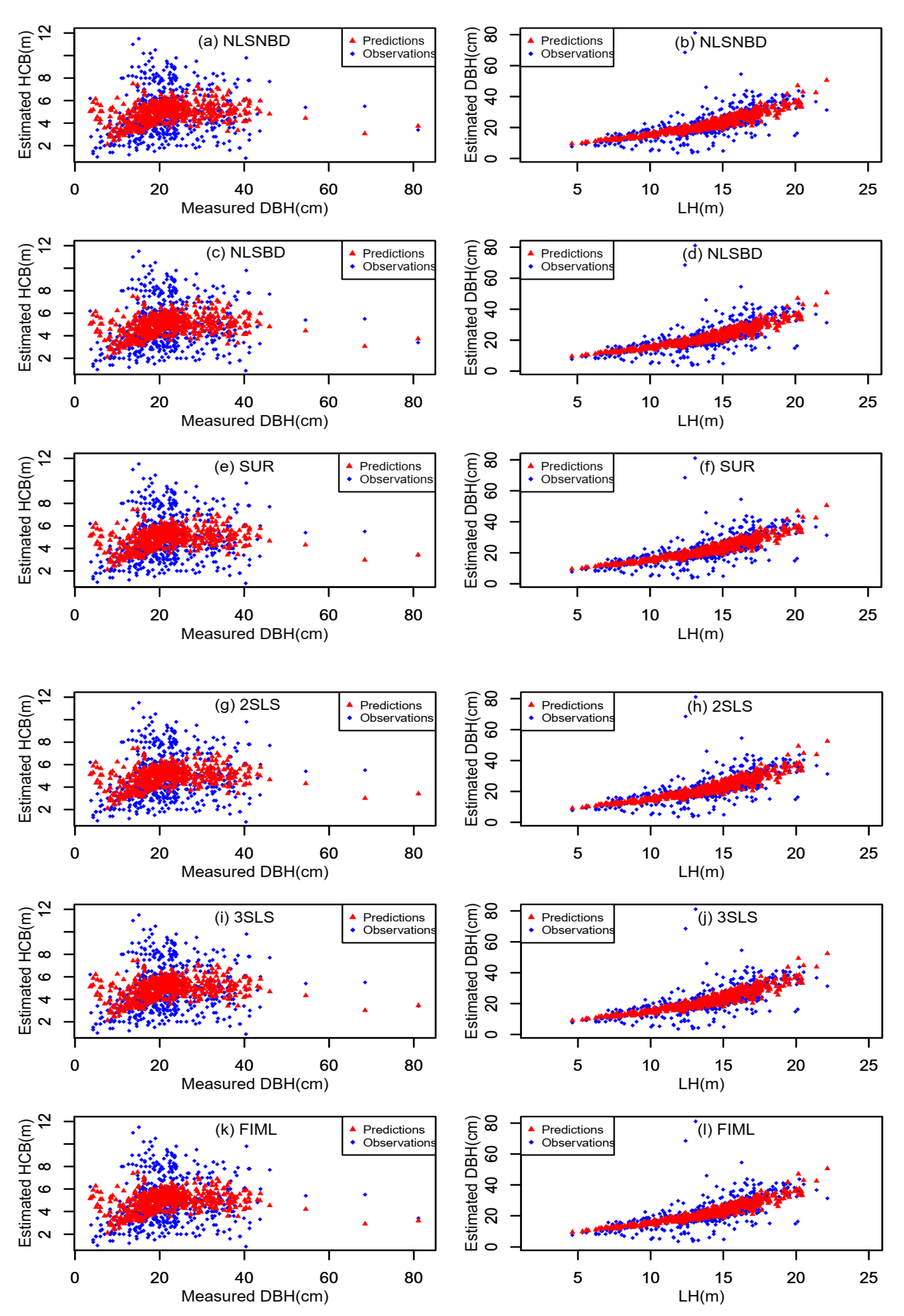
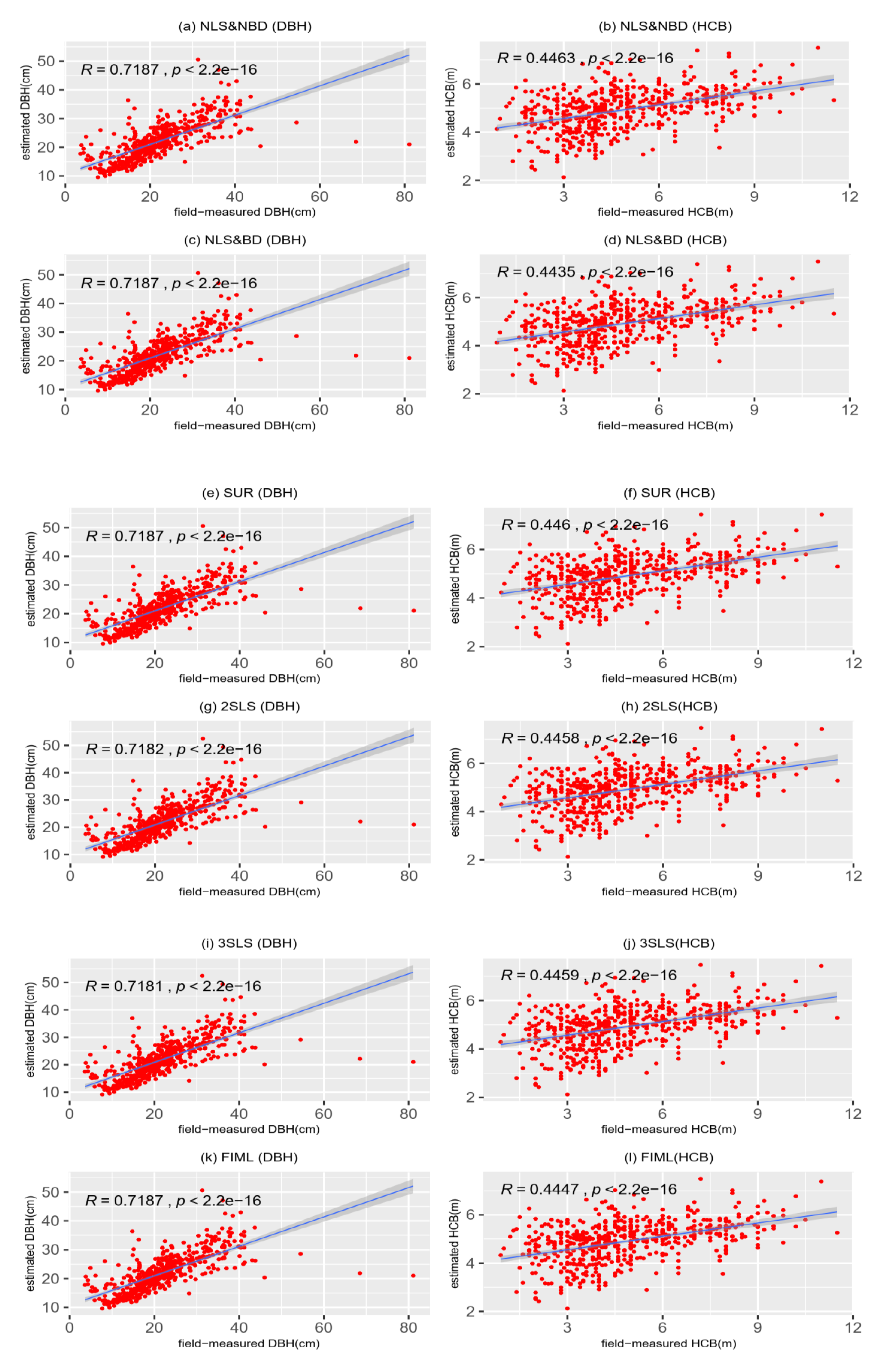
3.2. Model Prediction

The LOOCV was carried out for the LiDAR–DBH base model (Equation (1)), the LiDAR–HCB base model (Equation (2)), the NLS and NBD model (Equation (13)), and the NLS and BD model (Equation (16)) estimated using the nonlinear OLS, as well as the simultaneous equation system (Equation (3)) estimated using NSUR, 2SLS, 3SLS, FIML, and TSEM. The evaluations and comparisons of all these models were carried out using e ¯ , σ e 2 , and R M S E (Table 3).
A compatible DBH and HCB EIV equation system fitted with NSUR showed a better prediction ability than those fitted with other alternative methods (Table 3). For the DBH model, the σ e 2 of NSUR was identical to that of NSL and BD, as well as 0.37%, 0.37%, and 0.18% smaller than that of 2SLS, 3SLS, and FIML, respectively. The RMSE of NSUR was identical to that of NLS and BD, and it was 0.02%, 0.01%, and 0.08% smaller than that of 2SLS, 3SLS, and FIML, respectively. For the HCB model, the σ e 2 of NSUR was 0.35%, 0.021%, 0.006%, and 0.17% smaller than that of NLS and BD, 2SLS, 3SLS, and FIML, respectively. The RMSE of NSUR was 2.75%, 0.022%, 0.011%, and 0.082% smaller than that of NLS and BD, 2SLS, 3SLS, and FIML, respectively. The MAE of NSUR for HCB was the smallest.
The residuals of six different alternative models and equation systems were calculated based on a full dataset. This analysis indicated that the mean residuals of the NLS method for HCB were higher than other alternative methods, among which NSUR showed the smallest mean residual for HCB (Table 4).
The prediction accuracy of the simultaneous equation system (Equation (3)) fitted with all four fitting algorithms appeared almost identical (Figure 7), indicating that each of the fitting algorithms were able to produce almost equally unbiased estimations and prediction accuracies. The prediction accuracy of DBH seemed to be much higher than that of HCB.
The inherent correlations between the ground-measured DBH, model-estimated DBH, ground-measured HCB, and model estimated-HCB were all significantly high (Figure 8). The inherent correlation between DBH and HCB was substantially high. This figure suggested that all models and all fitting algorithms were appropriately suited to our data.

4. Discussion

HCB is an important tree attribute to assess tree productivity and tree vigor. DBH is commonly used to predict HCB model, but DBH estimated with LiDAR-based attributes contains unignorable errors. In addition, the compatibility between DBH and HCB needs to be considered when estimating HCB. In this study, we investigated four algorithms to estimate DBH and HCB in an EIV equation system—NSUR, 2SLS, 3SLS, and FIML—that were compared with two model structures. The prediction accuracy of the four EIV equation system algorithms and two model structures were reflected by RMSE and MAE. The results showed that the impacts of measurement error of DBH on HCB and the compatibility between DBH and HCB were well accounted for by the NSUR algorithm.
HCB is an important indicator for tree vigor and tree stem form, as well as an indispensable measure for retrieving the crown ratio. However, measuring in-situ HCB is quite labor-intensive and costly, especially when conducted for large forest areas. In this situation, an efficient method of obtaining precise HCB is necessary, which can be possible with the HCB prediction model developed from the LiDAR-derived variables, such as tree height, crown projection area, crown width, and ground-measured DBH. The first three variables can be relatively more accurately and easily measured by applying the advanced remote sensing techniques. The HCB can be estimated from the established HCB model, which may also contain DBH as a predictor [11,28]. The DBH estimation model can also be developed using the LiDAR-derived information [33]. The estimation of HCB and DBH from their corresponding prediction models would be substantially biased if separately developed models were used, i.e., DBH model and HCB models developed independently from each other from the same tree data. In order to overcome such a bias, developing a compatible simultaneous equation system is the most appropriate solution. However, this equation system of DBH and HCB models is still unavailable in forest modeling literature. As mentioned in the introduction, other compatible simultaneous equation systems developed through the EIV modeling approach are available, e.g., a system of equations of DBH and individual tree above-ground biomass models [33]. Considering the knowledge gap, we developed the simultaneous equation system of DBH and HCB models using the tree-level predictors (LH, LCW, and LCA), the information of which was derived from the LiDAR imagery. Four different algorithms (NSUR, 2SLS, 3SLS, and FIML) were used to estimate this equation system.
The data used in our study originated from the Picea crassifolia Kom forest, which is crucial to the economic and social benefits to the rural population, as well as regional carbon storage, regional carbon cycling, and the maintenance of the balanced-functions of forest ecosystems in northwest China. Two different model structures (the NLS and NBD model and the NLS and BD model) built by assuming errors associated with all the regressors and response variables were found to be inappropriate because this approach did not account for the inherent correlations of DBH with HCB and all the estimated parameters and variances were biased.
Generally, the structural estimators or fitting algorithms (NSUR, 2SLS, 3SLS, and FIML) should always be preferred to the NLS, as each of them effectively accounted for the errors in variables in an appropriate way. However, surprisingly, we found that NLS could sometimes provide a closer estimation of the structural estimators applied in this study, and it was the same for NLS and NBD. The NLS and NBD model had a smaller bias variance, so it has possibility to produce a smaller RMSE. However, NLS standard errors are, in all the likelihoods, not useful for inference purposes [57]. The prediction accuracy of the NLS and BD model was the worst with the highest σ e 2 and the biggest RMSE, thus, in this case, the EIV modeling approach clearly displayed the advantage over NLS. In general, individual tree DBH and HCB models based on the LiDAR data and field-measurements contain errors that exist in image capture, image processing, and the extraction of the information processes, and they are therefore very hard to completely avoid [29,33,58].
The NLS and NBD could neither address the compatibility problem of DBH and HCB nor account for their inherent correlations. However, a simultaneous equation system (Equation (3)) can effectively address these issues. Among the four algorithms used in fitting simultaneous equation system (Equation (3)), NSUR and 2SLS are classified into the limited information estimators, while 3SLS and FIML are the full information estimators. The former two estimators can make use of the reduced model information, while the latter two estimators can make use of full information from the model [33,34]. Based on the model validation results with LOOCV, the prediction accuracy of NSUR was slightly better than that of the other algorithms (2SLS, 3SLS, and FIML). This was probably because NSUR has a better ability to address the error transfers caused by DBH in the simultaneous equation system of the DBH and HCB models. Potentially because of this, Parresol [49] applied NSUR to develop the additive tree biomass models in a pioneer modeling study about a simultaneous equation system in forestry. The prediction accuracy of 3SLS was slightly better than 2SLS, confirming the findings of Tang et al. [34], who found that when errors in across equations were correlated, 3SLS outperformed 2SLS, and—when errors involved across equations were uncorrelated—2SLS outperformed 3SLS.
Our HCB equation system developed in this study was based on the most attractive fit statistics of the base model among the five frequently used HCB base candidate models [10,59,60]. The analysis of correlations between the regressors and HCB showed strong connections among LCA, LH, DBH, and HCB. In other words, these tree characteristics strongly influenced HCB variations. Our DBH base model, which replaced LCPA with LCW in the models of Fu et al. [33], showed a better fitting performance with a smaller RMSE. Both the HCB model applied with all the LiDAR-based data (except for DBH data, which were obtained from ground measurement) and the DBH model were developed by LiDAR data, and this enabled the DBH–HCB-compatible EIV models, suggesting the high possibility of the equation system’s application to an extensive forest area. The validation results based on the LOOCV for NSUR, 2SLS, 3SLS, and FIML were almost identical, even though NSUR slightly outperformed others; however, the prediction difference was still insignificant (Table 3). In this study, we only considered DBH and HCB as error-in-variables; however, other regressors may contain various errors including measurement errors, tree crown delineation errors, and errors of parameter estimation. Ignoring all these errors can cause the complex uncertainties while developing models. Future researchers should focus on these issues. Therefore, readers need to be cautious when considering the conclusion of this study.
As mentioned in the introduction section, this study was based on a novel methodology, which resulted in a system of compatible simultaneous equations of DBH and HCB models in which various LiDAR-derived tree attributes were used. The measurement errors of both DBH and HCB were simultaneously taken into consideration to address the problem of compatibility between DBH and HCB models and to account for inherent correlations between these tree variables through a simultaneous modeling approach. The presented equation system of DBH and HCB models can fulfill the gaps of the unavailability of such an HCB EIV model system in forest modeling literature. A compatible simultaneous equation system of the DBH and HCB models developed using the information of the tree-level predictors (LH, LCW, and LCA) derived from LiDAR imagery and ground-based measurements confirmed the accurate prediction of HCB and DBH. Compared to any of the previously developed HCB models using only ground measurements [11] and those based on LiDAR-derived databases [22,25,26,27,28], the presented equation system in this article will be interesting and useful to both researchers and forest managers, as this system is able to accurately predict HCB. Furthermore, the presented modeling approach and algorithm in this article will be useful for establishing similar compatible equation systems of DBH and HCB EIV models for other tree species and other tree variables that have inherent correlations between themselves.

5. Conclusions

This study developed a compatible simultaneous equation system of DBH and HCB EIV models on the basis of LiDAR-derived and ground-measured data of Picea crassifolia Kom trees in northwest China. Four different algorithms—NSUR, 2SLS regression, 3SLS regression, and FIML—were used to estimate the parameters in an equation system. The NLS used for estimating both the LiDAR–DBH base model (Equation (1)) and the LiDAR–HCB base model (Equation (2)) produced biased results, while the other fitting algorithms used for estimating a simultaneous equation system (Equation (3)) produced unbiased results with similar SSE, MSE, and RMSE. Two additional model structures—nonlinear least squares with HCB estimation not based on DBH (NLS and NBD) and nonlinear least squares with HCB estimation based on the DBH (NLS and BD)—were also developed for comparison. All the fitting algorithms and their resulting models were assessed by a leave-one-out cross validation method. This study indicates that only EIV modeling method can effectively account for the effects of errors associated with the regressors on the response variables and can guarantee the compatibility between DBH model and HCB model at the individual tree level. However, neither the NLS and BD model nor the NLS and NBD model exhibited these advantages. Among the various evaluated algorithms and models, NSUR showed a slightly better performance than the others. The results showed that the methodology proposed in this article is a reliable and efficient, and it can estimate individual tree DBH and HCB from LiDAR-based data over the extensive forest area. In addition, the presented simultaneous equation system (Equation (3)) does not need measurement of any stand-level variable, which would require an additional cost. The presented modeling approach and algorithm will be useful for establishing similar compatible equation systems of DBH and HCB EIV models for other tree species and other tree variables that have inherent correlations between themselves.

Author Contributions

Conceptualization, Z.Y., L.F., Q.L., Q.Y., H.Z., and G.D.; Formal analysis and writing-original draft preparation Z.Y., L.F., G.D., R.P.S., P.L., and G.W. All authors contributed to interpreting results and the improvement of the paper. All authors have read and agreed to the published version of the manuscript.

Funding

This research was funded by the Thirteenth Five-year Plan Pioneering project of High Technology Plan of the National Department of Technology (No. 2017YFC0504101), the Central Public interest Scientific Institution Basal Research Fund under (Grant No. CAFYBB2019QD003) and the Chinese National Natural Science Foundations (Grant Nos. 31570627 and 31570628).

Acknowledgments

We thank the National Program on Key Basic Research Project (973 Program) (No. 2007CB714400) for data support. We also appreciate the valuable comments and constructive suggestions from two anonymous referees and the Associate Editor.

Conflicts of Interest

The authors declare that they have no conflict of interest.

Appendix A

An R program for leave-one-out cross validation (LOOCV) using the SUR fitting algorithm is illustrated on full data set.
library(“openxlsx”)
library(systemfit)
mydata<- read.xlsx(“sample.xlsx”)
LOOCV<-function(mydata) {
N<-nrow(mydata)
EstD<-array(dim=N)
EstHCB<-array(dim=N)
start.values<-c(a0=5,a1=-0.1,a2=-0.1,b0=0.2, b1=0.1)
eqD<-DBH~(a0*exp(-a1*LH-a2*LCW))
eqHCB<-HCB~LH/(1+exp(b0*DBH+b1*LCA))
model<-list(eqD,eqHCB)
for (i in 1: N) {
Temp1<-mydata[-i,]
Temp2<-mydata[i,]
try (sur<-nlsystemfit (“SUR”, model, start.values, data=mydata), TRUE)
if(class(sur)==“try-error”)
{EstD[i]<-”NA”
EstHCB[i]<-”NA”}
else {
EstD[i]<-sur$b[1]*exp(-sur$b[2]*Temp2$LH-sur$b[3]*Temp2$LCW))
EstHCB[i]<-Temp2$LH/(1+exp(sur$b[4]*Temp2$DBH+sur$b[5]*Temp2$LCA))}
return (list (EstD,EstHCB))}

References

  1. Daniels, R.F.; Burkhart, H.E. Simulation of Individual Tree Growth and Stand Development in Managed Loblolly Pine Plantations; FWS-5-75; Division of Forestry and Wildlife Resources, Virginia Polytechnic and State University: Blacksburg, VA, USA, 1975; 69p. [Google Scholar]
  2. Navratil, S. Wind damage in thinned stands. In Proceedings of the A Commercial Thinning Workshop, Whitecourt, AB, Canada, 17–18 October 1997; pp. 29–36. [Google Scholar]
  3. Ancelin, P.; Courbaud, B.; Fourcaud, T. Development of an individual tree-based mechanical model to predict wind damage within forest stands. For. Ecol. Manag. 2004, 203, 101–121. [Google Scholar] [CrossRef]
  4. Dean, T.J.; Cao, Q.V.; Roberts, S.D.; Evans, D.L. MeaNSURing heights to crown base and crown median with LiDAR in a mature, even-aged loblolly pine stand. For. Ecol. Manag. 2009, 257, 126–133. [Google Scholar] [CrossRef]
  5. Scott, J.H.; Reinhardt, D. Assessing Crown Fire Potential by Linking Models of Surface and Crown Fire Potential; USDA Forest Service, Rocky Mountain Research: Washington, WA, USA, 2001.
  6. Hynynen, J. Predicting tree crown ratio model for Austrian forests. Can. J. For. Res. 1995, 25, 57–62. [Google Scholar] [CrossRef]
  7. Vauhkonen, J. Estimating crown base height for Scots pine by means of the 3D geometry of airborne laser scanning data. Int. J. Remote Sens. 2010, 31, 1213–1226. [Google Scholar] [CrossRef]
  8. Michael, E.D.; Burkhart, H.E. Compatible crown ratio and crown height models. Can. J. For. Res. 1987, 17, 572–574. [Google Scholar]
  9. Ritchie, M.W.; Hann, D.W. Equations for Predicting Height to Crown Base for Fourteen Tree Species in Southwest Oregon; Research Paper; Oregon State University, Forestry Research Laboratory: Corvallis, OR, USA, 1987. [Google Scholar]
  10. Baburam, R.; Aaron, R.; Weiskittel, J.A.; Kershaw, J. Development of height to crown base models for thirteen tree species of the North American Acadian Region. For. Chron. 2012, 88, 60–73. [Google Scholar] [CrossRef] [Green Version]
  11. Sharma, R.P.; Vacek, Z.; Vacek, S.; Podrázský, V.; Jansa, V. Modelling individual tree height to crown base of Norway spruce (Picea abies (L.) Karst.) and European beech (Fagus sylvatica L.). PLoS ONE 2017, 12, e0186394. [Google Scholar] [CrossRef] [PubMed] [Green Version]
  12. Fu, L.Y.; Sharma, R.P.; Hao, K.J.; Tang, S.Z. A generalized interregional nonlinear mixed-effects crown width model for Prince Rupprecht larch in northern China. For. Ecol. Manag. 2017, 389, 364–373. [Google Scholar] [CrossRef]
  13. Popescu, S.C. Estimating biomass of individual pine trees using airborne LiDAR. Biomass Bioenergy 2007, 31, 646–655. [Google Scholar] [CrossRef]
  14. Broadbent, E.N.; Asner, G.P.; Peña-Claros, M.; Palace, M.; Soriano, M. Spatial partitioning of biomass and diversity in a lowland Bolivian forest: Linking field and remote sensing measurements. For. Ecol. Manag. 2008, 255, 2602–2616. [Google Scholar] [CrossRef]
  15. Heurich, M. Automatic recognition and measurement of single trees based on data from airborne laser scanning over the richly structured natural forests of the Bavarian Forest National Park. For. Ecol. Manag. 2008, 255, 2416–2433. [Google Scholar] [CrossRef]
  16. Bi, H.; Fox, J.C.; Li, Y.; Lei, Y.; Pang, Y. Evaluation of nonlinear equations for predicting diameter from tree height. Can. J. Remote Sens. 2012, 42, 789–806. [Google Scholar] [CrossRef]
  17. Lefsky, M.A.; Cohen, W.B.; Acker, S.A.; Parker, G.G.; Spies, T.A.; Harding, D. LiDAR Remote Sensing of the Canopy Structure and Biophysical Properties of Douglas-Fir Western Hemlock Forests. Remote Sens. Environ. 1999, 70, 339–361. [Google Scholar] [CrossRef]
  18. Næsset, E. Predicting forest stand characteristics with airborne scanning laser using a practical two-stage procedure and field data. Remote Sens. Environ. 2002, 80, 88–99. [Google Scholar] [CrossRef]
  19. Pyysalo, U.; Hyyppä, H. Reconstructing tree crowns from laser scanner data for feature extraction. Int. Archives of Photogram. Remote Sens. Spat. Inf. Sci. XXXIV Part 3B 2002, 34, 218–221. [Google Scholar]
  20. Holmgren, J.; Persson, Å.; Söderman, U. Species identification of individual trees by combining high resolution LIDAR data with multi-spectral images. Int. J. Remote Sens. 2008, 29, 1537–1552. [Google Scholar] [CrossRef]
  21. Popescu, S.C.; Zhao, K. A voxel-based LiDAR method for estimating crown base height for deciduous and pine trees. Remote Sens. Environ. 2008, 112, 767–781. [Google Scholar] [CrossRef]
  22. Maltamo, M.; Bollandsås, O.M.; Vauhkonen, J.; Breidenbach, J.; Gobakken, T.; Næsset, E. Comparing different methods for prediction of mean crown height in Norway spruce stands using airborne laser scanner data. Forestry 2010, 83, 257–268. [Google Scholar] [CrossRef]
  23. Luo, L.; Zhai, Q.; Su, Y.; Ma, Q.; Kelly, M.; Guo, Q. Simple method for direct crown base height estimation of individual conifer trees using airborne LiDAR data. Opt. Express. 2018, 26, A562–A578. [Google Scholar] [CrossRef]
  24. Solberg, S.; Næsset, E.; Bollandsås, O.M. Single tree segmentation using airborne laser scanning data in a structurally heterogeneous spruce forest. Photogramm. Eng. Remote Sens. 2006, 72, 1369–1378. [Google Scholar] [CrossRef]
  25. Næsset, E.; Økland, T. Estimating tree height and tree crown properties using airborne scanning laser in a boreal nature reserve. Remote Sens. Environ. 2002, 79, 105–115. [Google Scholar] [CrossRef]
  26. Andersen, H.E.; McGaughey, R.J.; Reutebuch, S.E. Estimating forest canopy fuel parameters using LiDAR data. Remote Sens. Environ. 2005, 94, 441–449. [Google Scholar] [CrossRef]
  27. Maltamo, M.; Hyyppä, J.; Malinen, J. A comparative study of the use of laser scanner data and field measurements in the prediction of crown height in boreal forests. Scand. J. Forest Res. 2006, 21, 231–238. [Google Scholar] [CrossRef]
  28. Maltamo, M.; Karjalainen, T.; Repola, J.; Vauhkonen, J. Incorporating tree- and stand-level information on crown base height into multivariate forest management inventories based on airborne laser scanning. Silva Fennica 2018, 52, 1–18. [Google Scholar] [CrossRef]
  29. Zhang, W.; Ke, Y.; Quackenbush, L.J.; Zhang, L. Using error-in-variable (EIV) regression to predict tree diameter and crown width from remotely sensed imagery. Can. J. For. Res. 2010, 40, 1095–1108. [Google Scholar] [CrossRef]
  30. Rechenr, A.C.; Schaalje, G.B. Linear Models in Statistics, 2nd ed.; Woley: New York, NY, USA, 2008. [Google Scholar]
  31. Kangas, A.S. Effect of errors-in-variables on coefficients of a growth model and on prediction of growth. For. Ecol. Manag. 1998, 102, 203–212. [Google Scholar] [CrossRef]
  32. Carroll, R.J.; Ruppert, D.; Stefanski, L.A.; Crainiceanu, C.M. Measurement Error in Nonlinear Models: A Modern Perspective; Taylor & Francis Group LLC: New York, NY, USA, 2006; p. 438. [Google Scholar]
  33. Fu, L.Y.; Liu, Q.W.; Sun, H.; Wang, Q.Y.; Li, Z.Y.; Chen, E.X.; Pang, Y.; Song, X.Y.; Wang, G.X. Development of a system of compatible individual tree diameter and aboveground biomass prediction models using error-in-variable regression and airborne LiDAR data. Remote Sens. 2018, 10, 325. [Google Scholar] [CrossRef] [Green Version]
  34. Tang, S.; Li, Y.; Fu, L.Y. Statistical Foundation for Biomathematical Models, 2nd ed.; Higher Education Press: Beijing, China, 2015; p. 435. ISBN 978-7-04-042303-7. [Google Scholar]
  35. Fuller, W.A. Meansureement Error Models; John Wiley and Sons: New York, NY, USA, 1987. [Google Scholar]
  36. Tang, S.; Zhang, S. Measurement error models and their applications. J. Biomath. 1998, 13, 161–166. [Google Scholar]
  37. Tang, S.; Li, Y.; Wang, Y. Simultaneous equations, errors-invariable models, and model integration in systems ecology. Ecol. Model. 2001, 142, 285–294. [Google Scholar] [CrossRef]
  38. Lindley, D.V. Regression lines and the linear functional relationship. J. R. Stat. Soc. B 1947, 9, 218–244. [Google Scholar] [CrossRef]
  39. Tang, S.; Wang, Y. A parameter estimation program for the errors-in-variable model. Ecol. Model. 2002, 156, 225–236. [Google Scholar] [CrossRef]
  40. Walters, D.K.; Hann, D.W. Taper Equations for Six Conifer Species in Southwest Oregon; Forest Research Laboratory, Oregon State University: Corvallis, OR, USA, 1986; p. 41. [Google Scholar]
  41. Pang, Y.; Chen, E.; Liu, Q.; Xiao, Q.; Zhong, K.; Li, X.; Ma, M. WATER: Dataset of airborne LiDAR mission at the super site in the Dayekou watershed flight zone on Jun. 23, 2008. In Chinese Academy of Forestry; Institute of Remote Sensing Applications, Chinese Academy of Sciences; Cold and Arid Regions Environmental and Engineering Research Institute, Chinese Academy of Sciences; Heihe Plan Science Data Center: Lanzhou, China, 2008. [Google Scholar]
  42. Koch, B.; Heyder, U.; Weinacker, H. Detection of Individual Tree Crowns in Airborne Lidar Data. Photogramm. Eng. Remote Sens. 2006, 72, 357–363. [Google Scholar] [CrossRef] [Green Version]
  43. Parent, J.R.; Volin, J.C. Assessing the potential for leaf–off LiDAR data to model canopy closure in temperate deciduous forests. Photogramm. Eng. Remote Sens. 2014, 95, 134–145. [Google Scholar] [CrossRef]
  44. Liu, Q.; Fu, L.; Wang, G.; Li, S.; Li, Z.; Chen, E.; Pang, Y.; Hu, K. Improving estimation of forest canopy cover by introducing loss ratio of laser pulses using airborne LiDAR. IEEE Trans. Geosci. Remote. 2020, 58, 567–584. [Google Scholar] [CrossRef]
  45. Liu, Q. Study on the Estimation Method of Forest Parameters Using Airborne Lidar. Ph.D. Thesis, Chinese Academy of Forestry, Beijing, China, 2009. (In Chinese). [Google Scholar]
  46. Liu, Q.; Li, Z.; Chen, E.; Pang, Y.; Wu, H. Extracting individual tree heights and crowns using airborne LIDAR data. J. Beijing For. Univ. 2008, 30, 83–89. [Google Scholar]
  47. Fu, L.; Lei, Y.; Wang, G.; Bi, H.; Tang, S.; Song, X. Comparison of seemingly unrelated regressions with multivariate errors-in-variables models for developing a system of nonlinear additive biomass equations. Trees 2016, 30, 839–857. [Google Scholar] [CrossRef]
  48. Parresol, B.R. Assessing tree and stand biomass: A review with examples and critical comparisons. For. Sci. 1999, 45, 573–593. [Google Scholar]
  49. Parresol, B.R. Additivity of nonlinear biomass equations. Can. J. For. Res. 2011, 31, 865–878. [Google Scholar] [CrossRef]
  50. Judge, G.G.; Hill, R.C.; Griffifiths, W.E.; Lutkepohl, H.; Lee, T.C. Introduction to the Theory and Ractice of Econometrics, 2nd ed.; Wiley: New York, NY, USA, 1988. [Google Scholar]
  51. Zellner, A.; Theil, H. Three Stage Least Squares: Simultaneous Estimation of Simultaneous Equations. Econometrica 1962, 30, 54–78. [Google Scholar] [CrossRef]
  52. Fumio, H. Econometrics; Shanghai University of Finance and Economics Press: Shanghai, China, 2005; p. 536. ISBN 7-81098-499-3. [Google Scholar]
  53. Nord-Larsen, T.; Meilby, H.; Skovsgaard, J.P. Site-specific height growth models for six common tree species in Denmark. Scand. J. For. Res. 2009, 24, 194–204. [Google Scholar] [CrossRef]
  54. Timilsina, N.; Staudhammer, C.L. Individual tree-based diameter growth model of slash pine in Florida using nonlinear mixed modeling. For. Sci. 2013, 59, 27–31. [Google Scholar] [CrossRef]
  55. Zhao, D.; Lynch, T.B.; Westfall, J.; Coulston, J.; Kane, M.; Adams, D.E. Compatibility, development and estimation of taper and volume equation systems. For. Sci. 2019, 65, 1–13. [Google Scholar] [CrossRef] [Green Version]
  56. R Core Team. R: A Language and Environment for Statistical Computing; R Foundation for Statistical Computing: Vienna, Austria, 2018; Available online: https://www.R-project.org/ (accessed on 15 March 2020).
  57. Greene, W.J. Econometric Analysis, 7th ed.; Pearson Education, Inc.: New York, NY, USA, 2001; p. 1188. ISBN 0-13-139538-6. [Google Scholar]
  58. Curran, P.J.; Hay, A.M. The importance of mesauement error for certain procedures in remote sensing at optical wavelengths. Photogramm. Eng. Remote Sens. 1986, 52, 229–241. [Google Scholar]
  59. Wykoff, W.R. A basal area increment model for individual conifers in the northern Rocky Mountains. For. Sci. 1990, 136, 1077–1104. [Google Scholar]
  60. Van Deusen, P.C.; Biging, G.S. STAG, A Stand Generator for Mixed Species Stands; Research Note; Northern 55 California Forest Yield Cooperative, Department of Forestry and Resource Management, University of California: Berkeley, CA, USA, 1985; Volume 11, 25p. [Google Scholar]
Figure 1. (a) Location of the study site: Xishui forest farm located in the Su’nan Yuguzu autonomous county of the Gansu Qilian Mountains National Nature Reserve, Western China and (b) tree positions within 16 sub-sample plots nested within a permanent sample plot of 100 × 100 m.
Remotesensing 12 02238 g001
Figure 2. The relationships of height to crown base (HCB) with other tree variables: (a) light detection and ranging (LiDAR)-derived tree height (LH), (b) crown width (LCW), (c) diameter at breast height (DBH), and (d) crown projection area (LCA) for Picea crassifolia Kom.
Remotesensing 12 02238 g002
Figure 3. Correlations between LiDAR-derived HCB and ground-measured HCB (a), correlation between LiDAR-derived tree height and ground-measured tree height (b), correlation between LiDAR-derived crown with and ground-measured crown width (c), and correlation between LiDAR-derived crown area and ground measured crown area (d).
Remotesensing 12 02238 g003
Figure 4. Predicted HCB (m) of trees against y-coordinate Y (m) located within coordinate X (608,960–608,970 m).
Remotesensing 12 02238 g004
Figure 5. Digital elevation model (DEM) of sample plot (a) and footprint of laser pulse (b).
Remotesensing 12 02238 g005
Figure 6. A flow chart depicting a brief description of four algorithms (NSUR, nonlinear seemingly unrelated regression; 2SLS, two-stage least square; 3SLS, three-stage least square; and FIML, full information maximum likelihood) used to estimate a DBH and HCB error-in-variable (EIV) equation system.
Remotesensing 12 02238 g006
Figure 7. Scattered plots of estimated values of HCB versus ground-measured DBH for nonlinear least squares with HCB estimation not based on DBH (NLS and NBD) (a), nonlinear least squares with HCB estimation based on the DBH (NLS and BD) (c), NSUR (e), 2SLS regression (g), 3SLS regression (i), and FIML (k). Scattered plots of estimated DBH versus LH for NLS and NBD (b), NLS and BD (d), NSUR (f), 2SLS (h), 3SLS (j), and FIML (l).
Remotesensing 12 02238 g007
Figure 8. Correlations between the ground-measured tree diameter at breast height (DBH) and estimated DBH for nonlinear least squares with height to crown base (HCB) estimation not based on DBH (NLS and NBD) (a), nonlinear least squares with HCB estimation based on the DBH (NLS and BD) (c), NSUR (e), 2SLS regression (g), 3SLS regression (i), and FIML (k), as well as correlations between ground-measured tree HCB and estimated HCB from NLS and NBD (b), NLS and BD (d), NSUR (f), 2SLS (h), 3SLS (j), and FIML (l). R = Pearson’s correlation coefficient.
Remotesensing 12 02238 g008
Table 1. Descriptive statistics of tree measurements (SD, standard deviation).
VariableMin.Max. MeanSD
LH (m)4.6222.1513.843.20
HCB (m)0.9010.204.803.52
LCW (m)2.007.504.200.95
DBH (cm)3.6081.1022.578.54
LCA (m)3.1938.6312.215.47
Table 2. Parameter estimates of the LiDAR–DBH base model (Equation (1)), the LiDAR–HCB base model (Equation (2)), and the NLS and BD model (Equation (13)), as well as the simultaneous equation system (Equation (3)). The first three models were estimated using ordinary least squares regression, and the last one was estimated using NSUR, 2SLS, 3SLS, and FIML.
ModelMethodParametersEstimatesStandard Errort-Value
LiDAR–DBH base model (Equation (1))NLS β 1 5.71610.359915.882
β 2 −0.05670.0061−9.344
β 3 −0.12640.0178−7.108
σ 2 37.22
LiDAR–HCB base model (Equation (2))NLS γ 1 0.00530.00311.68
γ 2 0.03670.00576.4340
σ 2 3.37
HCB based on DBH model (Equation (13))NLS μ 1 −0.00030.0547−0.00
NLS and BD μ 2 0.24720.1987−1.24
μ 3 0.08000.05201.54
μ 4 0.02830.01372.07
σ 2 3.33
Simultaneous equation system (Equation (3))NSUR β 1 5.69920.361515.77
β 2 −0.05630.0061−9.27
β 3 −0.12830.0180−7.12
γ 1 0.00590.00321.87
γ 2 0.03610.00586.26
σ D B H 2 37.22
σ H C B 2 3.32
σ D H 0.608
Simultaneous equation system (Equation (3))2SLS β 1 5.24960.358614.64
β 2 −0.05670.0064−8.83
β 3 −0.14510.0186−7.80
γ 1 0.00540.00511.04
γ 2 0.03700.00914.08
σ D B H 2 37.93
σ H C B 2 3.32
σ D H 0.551
Simultaneous equation system (Equation (3))3SLS β 1 5.26410.359014.66
β 2 −0.05640.0064−8.78
β 3 −0.14570.0186−7.83
γ 1 0.00520.00511.01
γ 2 0.03730.00914.12
σ D B H 2 37.88
σ H C B 2 3.32
σ D H 0.553
Simultaneous equation system (Equation (3))FIML β 1 5.70360.346916.44
β 2 −0.05610.0047−11.84
β 3 −0.12890.0149−8.66
γ 1 0.00740.00421.76
γ 2 0.03350.00764.39
σ D B H 2 37.72
σ H C B 2 3.31
σ D H 0.65
Table 3. Prediction statistics of the models: the DBH-based model (Equation (1)), the HCB-based model (Equation (2)) fitted with NLS, the HCB based on DBH model (Equation (13)) fitted with NLS, and the simultaneous equation system (Equation (3)) fitted with the NSUR, 2SLS regression, 3SLS regression, and FIML algorithms.( e ¯ , mean bias;   σ e 2 , bias variance; and R M S E , root mean square error. All other acronyms are the same as defined in Table 2).
Fitting MethodVariables e ¯ σ e 2 RMSEMAE
NLS and NBDDBH−0.042637.65726.13673.6998
HCB−0.03673.33871.82761.4619
NLS and BDHCB−0.41863.35301.87841.4619
NSUR DBH−0.045837.65776.13683.7008
HCB−0.02763.34141.82811.4606
2SLS DBH0.009337.79856.14813.6984
HCB−0.03363.34211.82851.4612
3SLS DBH0.002637.79776.14803.7004
HCB−0.03413.34161.82831.4613
FIML DBH−0.045737.65986.13693.7012
HCB−0.01953.34701.82961.4613
Table 4. Descriptive statistics of residuals of the LiDAR– DBH base model (Equation (1)), LiDAR–HCB base model (Equation (2)), and model (Equation (13)), and simultaneous equation system (Equation (3)). The first three models were estimated using ordinary least squares regression and last one was estimated using NSUR, 2SLS, 3SLS, and FIML. (SD, standard deviation).
ModelMethodResponse VariableMin. of ResidualsMax. of ResidualsMean of ResidualsSD of Residuals
LiDAR–DBH base model (Equation (1))NLSDBH−60.099221.60270.04236.1365
LiDAR–HCB base model (Equation (2))NLSHCB−6.17054.34870.03671.8272
HCB based on DBH model, NLS and BD (Equation (13))NLSHCB−6.17084.34950.03421.8300
Simultaneous equation system (Equation (3))NSURDBH−60.088321.58310.04586.1366
HCB−6.20684.40990.02761.8279
Simultaneous equation system (Equation (3))2SLSDBH−60.113222.2219−0.00936.1481
HCB−6.21934.40610.03361.8282
Simultaneous equation system (Equation (3))3SLSDBH−60.087422.1638−0.00266.1480
HCB−6.21504.39990.03411.8280
Simultaneous equation system (Equation (3))FIMLDBH−60.081921.57100.04576.1368
HCB−6.24074.46680.02951.8295

