1. Introduction
During the first half of 2020, the world experienced economic collapse due to the COVID-19 pandemic since the Great Depression in the late 1920s [
1]. It is well established that low-light imaging satellite sensors are able to detect the dimming and loss of lighting after disaster events [
2,
3,
4], wars [
5,
6], and economic collapse [
7]. In order to explore the possibility that satellite observation can be used to track the decline and recovery of economic activity worldwide associated with the COVID-19 pandemic, we conducted an analysis of lighting changes in China, the first country that experienced the pandemic. Large portions of the Chinese economy shut down, as the government imposed a national lockdown forcing most people to remain at home [
8]. Previous satellite studies indicate that the nighttime lights of China have been growing for several decades [
9]. For this study, we use specialized low-light imaging satellite data collected by the NASA/NOAA Visible Infrared Imaging Radiometer Suite (VIIRS) day-night band (DNB). The DNB light intensification was designed to detect moonlit clouds in the visible band [
10]. With a million-fold amplification in the signal, the DNB also detects electric lighting present at the Earth’s surface.
Because clouds can block the detection of surface lighting, many scientists interested in using satellites to observe nighttime lights choose to work with cloud-free temporal composites. Annual cloud-free composites have sufficient temporal leverage to fill in seasonal data outages from sunlight and to filter out ephemeral features unrelated to electric lighting [
11]. These include biomass burning and energetic particle hits from the aurora and the South Atlantic Anomaly. In some cloud-prone areas, such as Java Island, it takes a full year to get a sufficient number of cloud-free observations to generate a sharp and clear image of nighttime lights. However, in cases where the user wishes to study short–term changes in lighting, the phenomena of interest are averaged away and cannot be seen clearly in an annual average. In such a case, monthly and nightly data products are available and can be considered for use. Studies conducted with nightly images are well suited for small geographic extents, where an analyst can select sets before and after images that are cloud-free. Another way to work with nightly data is to assemble temporal profiles for individual locations and then filter out clouds or cloud plus moonlight. The monthly composites differ from the annual VIIRS nighttime lights products, in that they are not filtered to remove ephemeral events, like biomass burning. In addition, background areas having no detectable lighting are not zeroed out in the monthly composites. It is left to the user to perform filtering based on their use case.
This analysis is based primarily on two pairs of monthly cloud-free composites and the sum of the light brightness for 300+ level 2 administrative units [
12] in each of four months. For the subject pair, we used the composites of December 2019 and February 2020 and calculated the percentage change in brightness in February relative to that in December 2019. The composites in December 2019 were selected, because December 2019 is the last full month prior to the public recognition of the outbreak in January. We intentionally skipped over January 2020 to avoid lighting changes associated with the Chinese New Year (CNY), which fell on 25 January 2020. During the CNY, many institutions close for two weeks centered on the New Year date, and many people return to their provinces. To avoid any possible CNY effects, we selected the February 2020 composite set for the analysis, corresponding to the peak lockdown period. To provide a reference, the same analysis was performed on a pair of months from the previous year: December 2018 and March 2019. The February 2019 composite was skipped in favor of March 2019, because the CNY in 2019 was on February 5.
The monthly composites include a pair of images—the average radiance and the tally of cloud-free coverages. Radiance difference images were calculated and used to produce colorized maps for specific cities. In addition, we calculated the percentage change in brightness for more than 300 level 2 administrative units [
12]. The grid cell set used for the four months in the % change calculation was standardized by blocking grid cells having low cloud-free coverages or extremely low radiances. Then, the radiances were summed for each administrative unit. These sums were then differenced, and a percent difference was calculated.
In addition, we examined the evidence of dimming in a nightly temporal profile to show how the exact start dates of dimming and the level of recovery can be derived as well as an assessment of the lighting recovery level.
2. Materials and Methods
We presented results from three different styles of DNB data products: filtered monthly composites, temporal profiles from monthly composites, and a nightly temporal profile. The one we spent the most time on were the two monthly pairs (December 2018 to March 2019 and December 2019 to February 2020). Here, we filtered the composites to extract a consistent set of lit grid cells for the comparison of the pre-pandemic brightness levels and the dimming of lights during the pandemic. The percent of dimming during the pandemic was then checked against the report confirming COVID-19 infections published by the Harvard Dataverse [
13]. We then presented results from the entire time series of cloud-free composites to check whether the pandemic dimming was unique. Finally, we presented a nightly temporal profile to identify dates for the onset of dimming and recovery, plus the recovery level relative to the pre-pandemic brightness level.
Preparation of the two monthly pairs: The methods used to generate monthly cloud-free average radiances were described by Elvidge et al. [
11]. These were rough composites; in that they were not filtered to remove background or biomass burning. The key to using the monthly products to analyze the dimming of lights across administrative units was to mask out background and poor-quality data, focusing the analysis on a consistent set of lit grid cells from each of the four focus months. In this case, we filtered the composites based on low cloud-free coverages, low radiance levels, and snow cover.
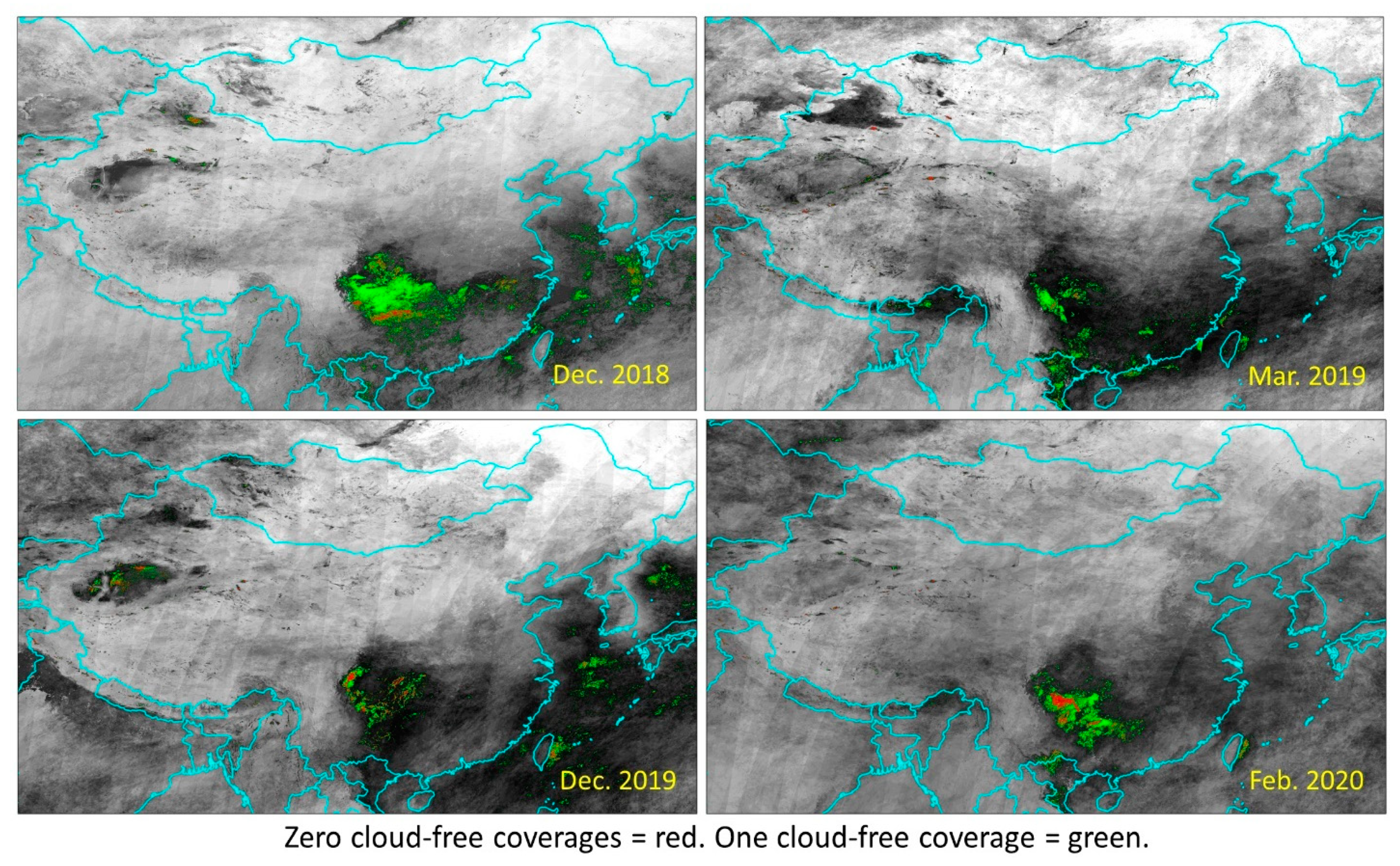
Filtering on low cloud-free coverages: We visually examined the cloud-free coverage grids for China and found there were data gaps with zero cloud-free coverages in every month (
Figure 1). In addition, we decided to filter out grid cells having single cloud-free coverages and focused the study on areas having larger numbers of usable observations. For each month, a binary on-off mask was generated for grid cells having less than two cloud-free coverages. The final mask for low cloud-free coverages was set, so that a grid cell was excluded from the study if it dipped below two cloud-free coverages in any of the four months.
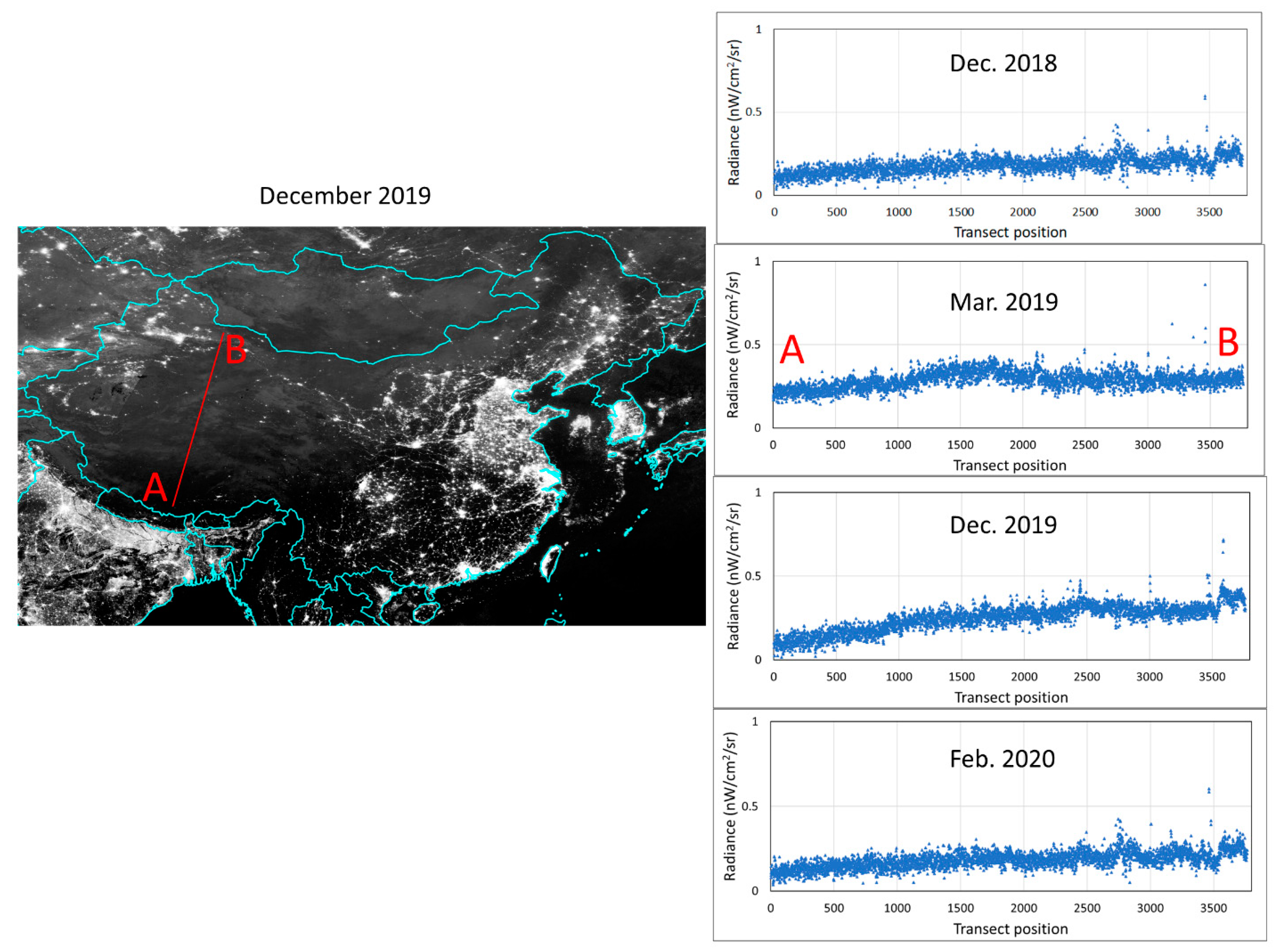
Filtering based on low average radiance: We filtered out grid cells that dipped below one nW/cm
2/sr in any of the four months. This filtering had two primary purposes. The first was to zero out background areas, where no lighting was detected. Although the average radiance in background areas was quite low, it varied both spatially and temporally (
Figure 2). In many of China’s western provinces, the areas of lighting are dwarfed by the spatial extent of the background. If the background radiances are summed with the lights, the result will be dominated by the temporal variations in the background. The other reason to filter based on low average radiance was to eliminate biomass burning. Fires are quite bright in the DNB; however, they typically occur in background areas lacking electric lighting detectable by VIIRS. Biomass burning was filtered from the four study months by filtering out grid cells that dipped below one nW in any of the four months.
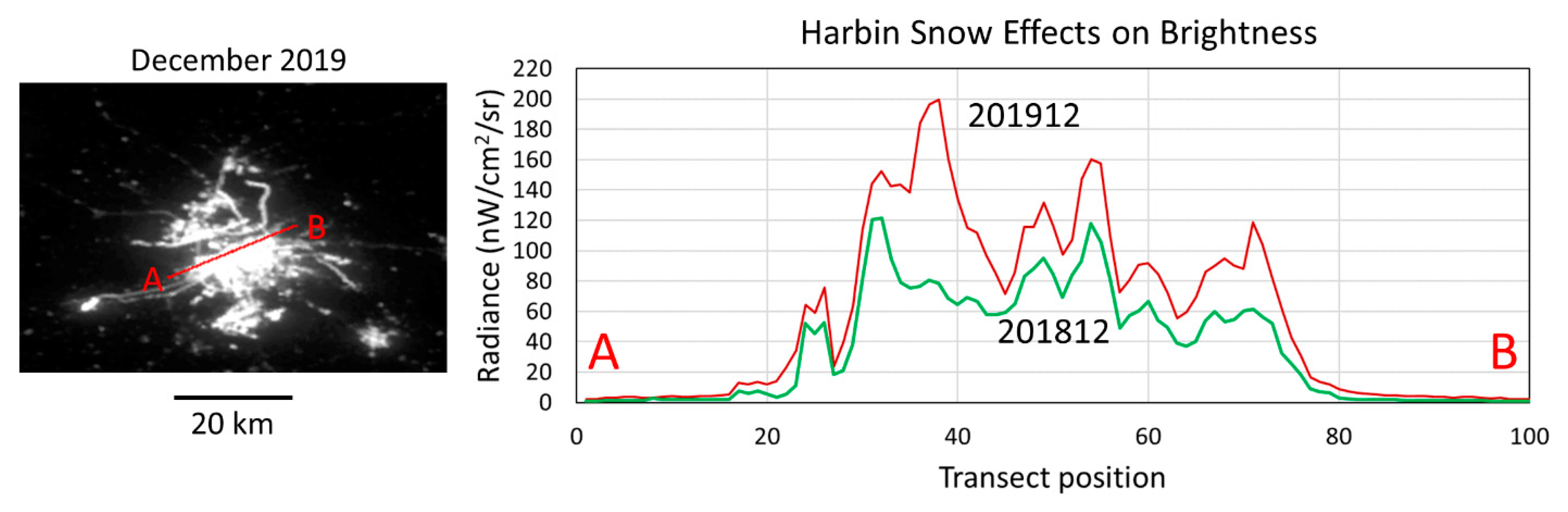
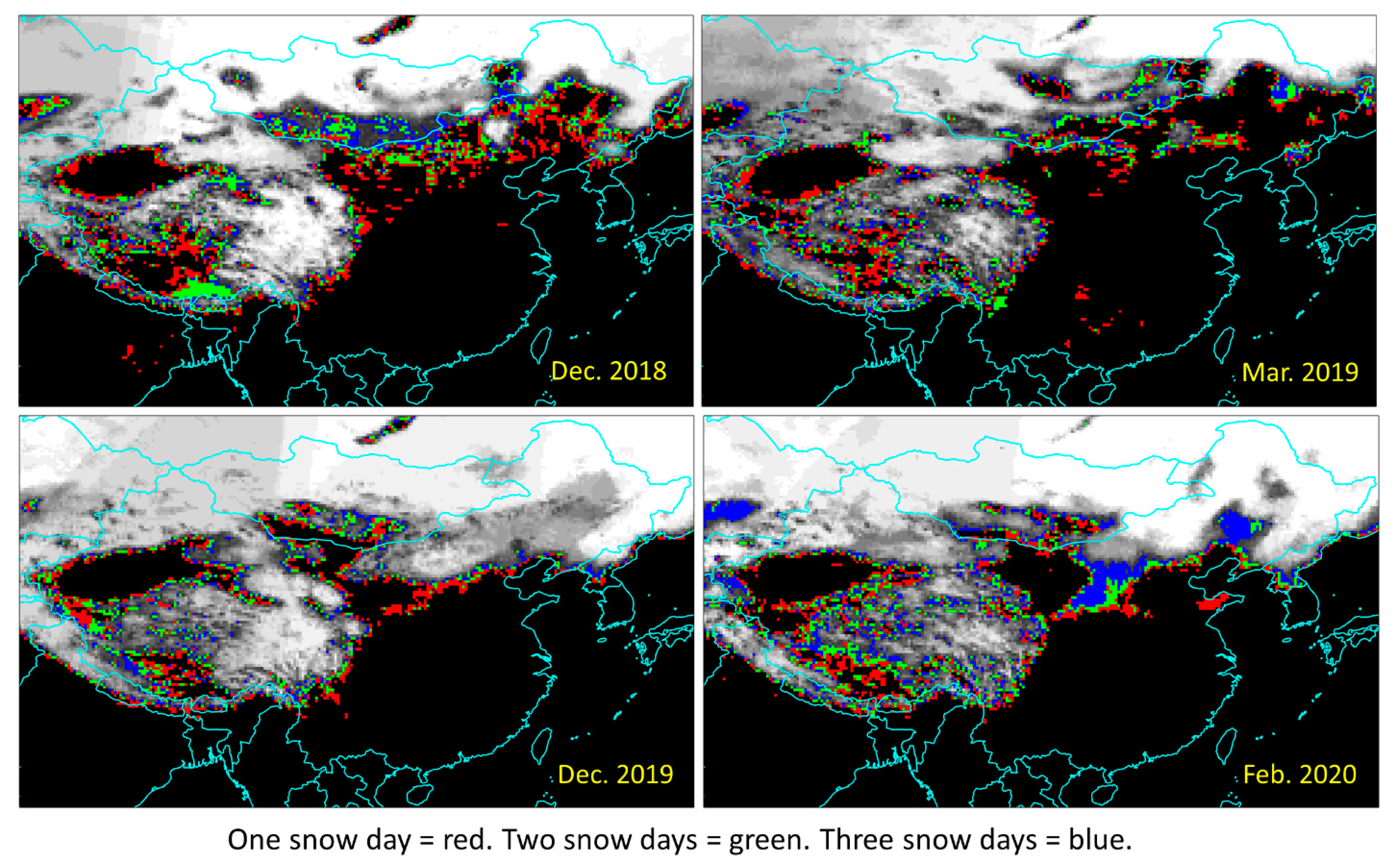
Filtering of snow cover: The high visible wavelength reflectivity of snow increased the brightness of lighting observed by satellite.
Figure 3 shows an example of snow–induced brightening along a transect through Harbin, China, where snow was absent in December 2018 but consistently present during the December 2019 compositing period. The December 2018 radiance was consistently dimmer than the December 2019 levels. At present, there is no technique for removing snow effects. Therefore, grid cells having snow cover in any of the four months were excluded from the change detection analysis. A snow cover mask was produced for each of the four months using NOAA Advanced Microwave Sounding Unit-A (AMSU-A) daily snow cover product [
14], tallying the number of times snow cover was detected for the same set of days used in the DNB cloud-free composites (
Figure 4). Monthly snow cover tallies of one and two were filtered out to remove false detections. This removed a narrow rim of AMSU-A detections surrounding the consistently snow-covered areas. Then, the four monthly snow products were added together to generate a mask used to zero out lighting affected by snow cover in any of the four months.
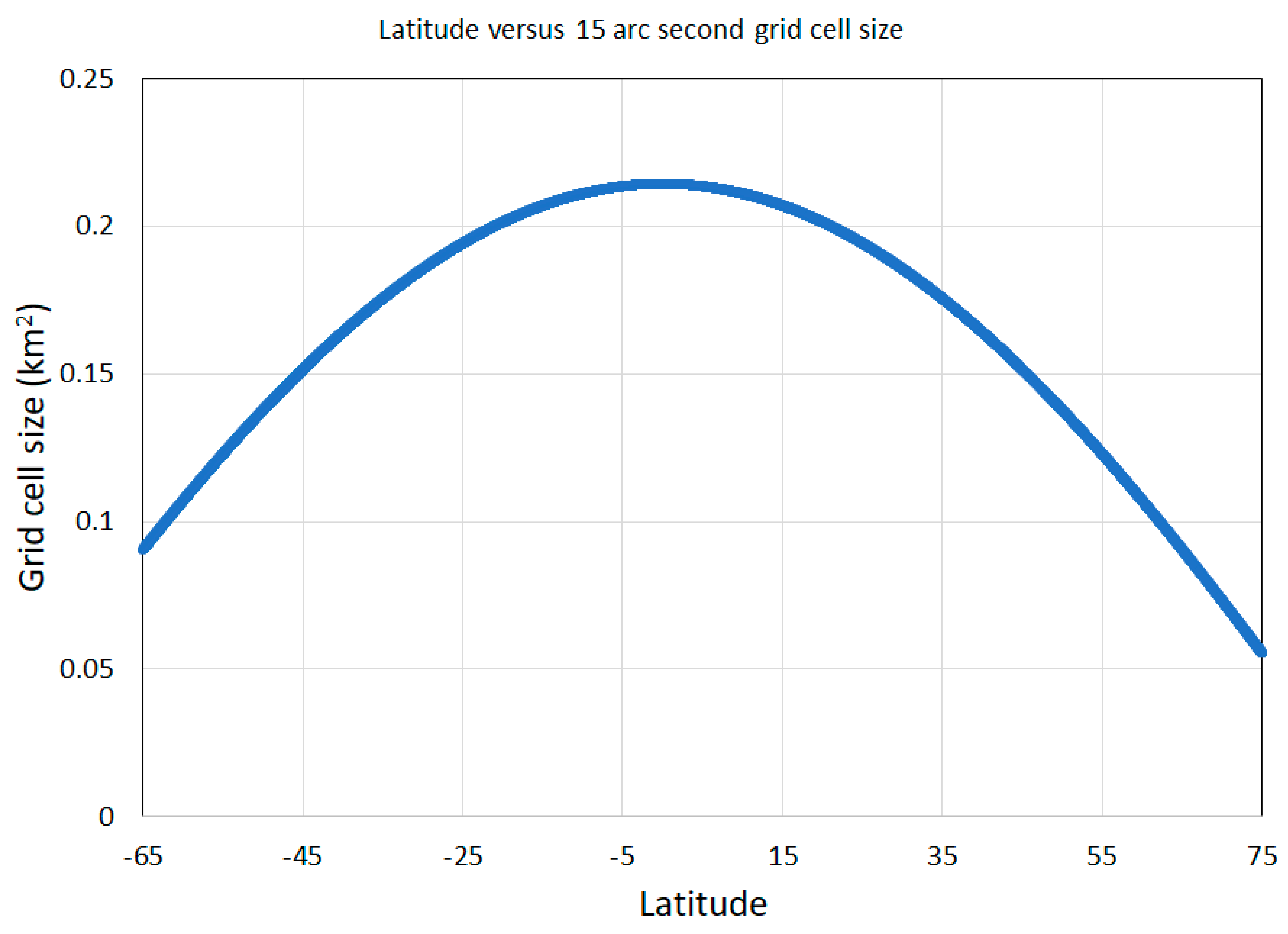
Sum-of-lights (SOL) calculation: After masking, the radiances of the remaining grid cells were multiplied by the surface area of 15 arc-second grid cells prior to summing inside the level 2 administrative units. This “latitude adjustment” was necessary, because the ground footprint of the grid cells declined with latitude (
Figure 5). The grid cells at the equator covered 0.857 km
2 and decreased with latitude, following a cosine function [
15]. China spans latitudes from 18 to 53°N. Therefore, in the south, the grid cells cover 0.204 km
2, and in the far north they only cover 0.129 km
2. The SOL was calculated by summing the grid cell radiance inside the level 2 administrative units after the latitude adjustment. These sums were then differenced, and a percent difference was calculated. The population of the administrative units was tallied with the Landscan population grid from 2018 [
16] along with a latitude adjustment.
3. Results
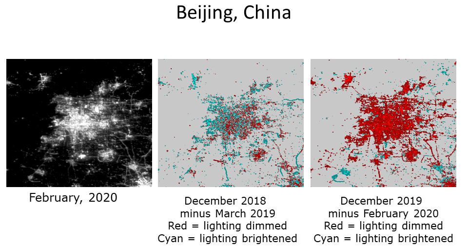
Colorized difference images: To consider initial COVID-19 effects, we examined the change in brightness between the two monthly pairs for several major urban areas in China. By coloring gains in brightness as cyan and declines in brightness as red, it was possible to compare the color patterns for the pre-pandemic pair (December 2018 and March 2019) and the pair that straddled the pandemic lockdown (December 2019 and February 2020).
Figure 6 shows results for five major urban areas: Wuhan, Beijing, Guangzhou, Shanghai, and Xi’an. It can be seen in all five areas that there was generally a mix of dimming and brightening in each monthly pair. Brightening dominates in the pre-pandemic pair. In contrast, the lockdown pairs showed extensive areas experienced a decline in brightness in February 2020. For Wuhan, there was a relatively even mix of increase and decline in brightness for February 2020. This qualitative observation was confirmed by the quantitative analysis results in
Table 1, which shows Wuhan lighting increased by 8% in the pre-pandemic pair and declined by 3% during the lockdown period. The decline in lockdown lighting appeared much more substantial in Beijing (
Figure 6), and this was confirmed by the results in
Table 1, where the city’s lighting increased by 3% in the reference pair but declined by 24% during the lockdown. Shanghai and Guangzhou fell between Wuhan and Beijing in terms of the diming of lights, both witnessing a 12% decline during the lockdown. Xi’an also showed extensive areas of dimming during the lockdown period. The quantitative results in
Table 1 showed Xi’an’s light brightness grew by 23% during the reference period and declined by 19% during the lockdown.
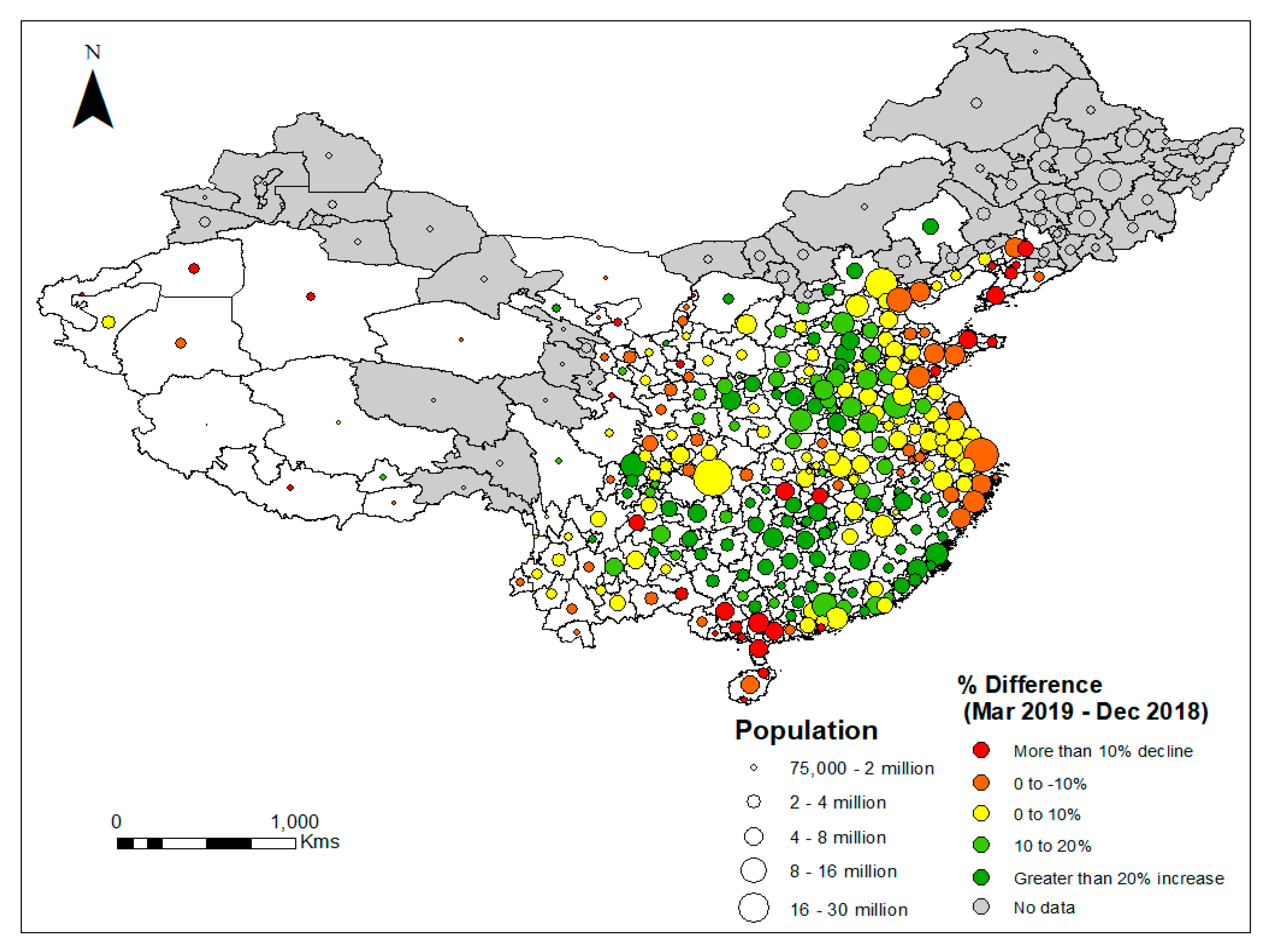
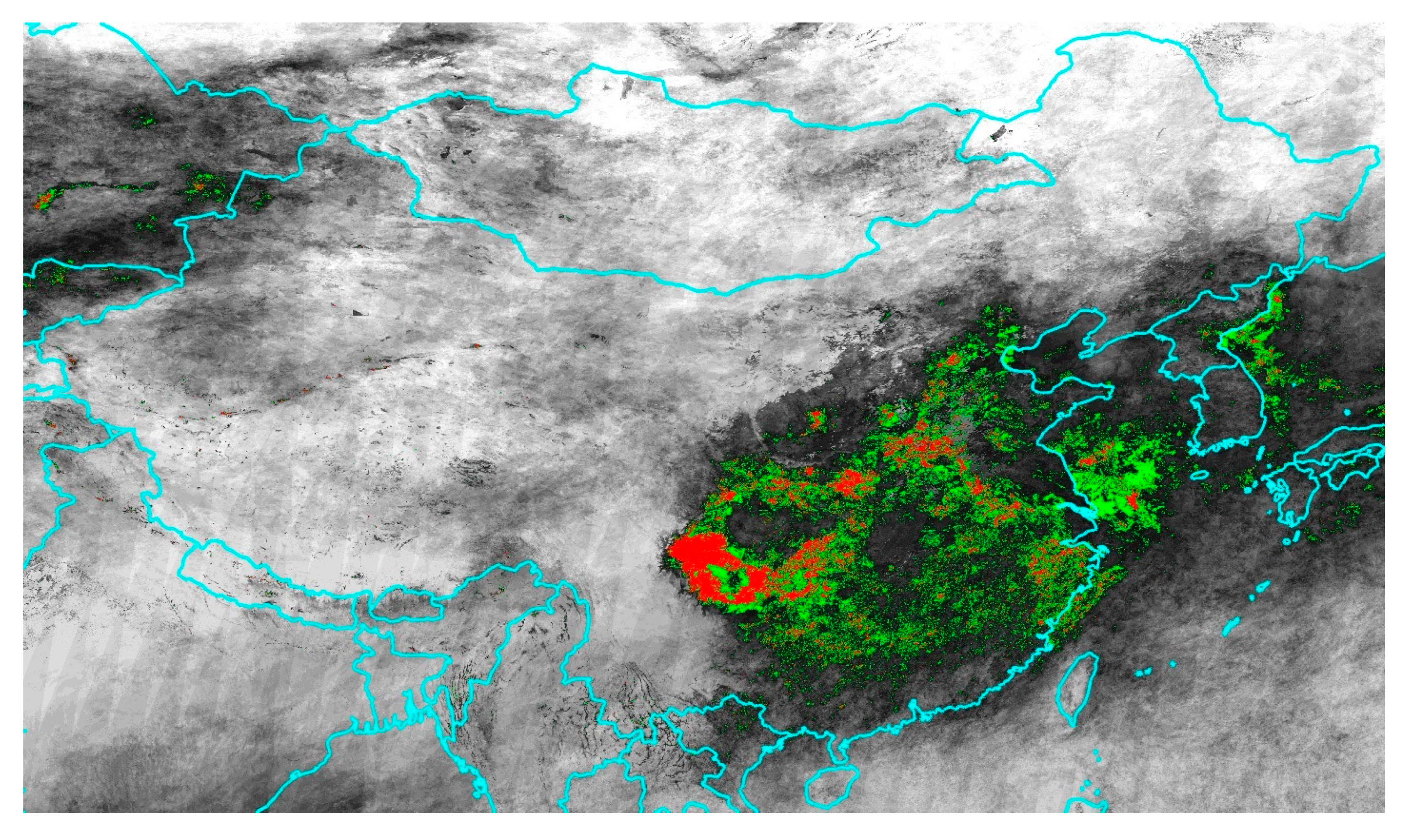
Percent change maps with population: A pair of maps were created to spatially visualize the change in brightness across the entire country in reference to population numbers (
Figure 7 and
Figure 8). The maps show the outlines of the subnational units and have circles with different sizes based on population and color coded to five classes of change in brightness. There were three color-coded classes for increased brightness: yellow, light green, and dark green. There were two color-coded classes for declines in brightness: orange and red. The pre-pandemic reference (
Figure 7) set showed that the heavily populated areas in Central China had yellow and green circles predominating, indicating that growth in lighting was widespread. In contrast, the pandemic map (
Figure 8) shows the predominance of orange and red circles, indicating the prevalence of declines in lighting.
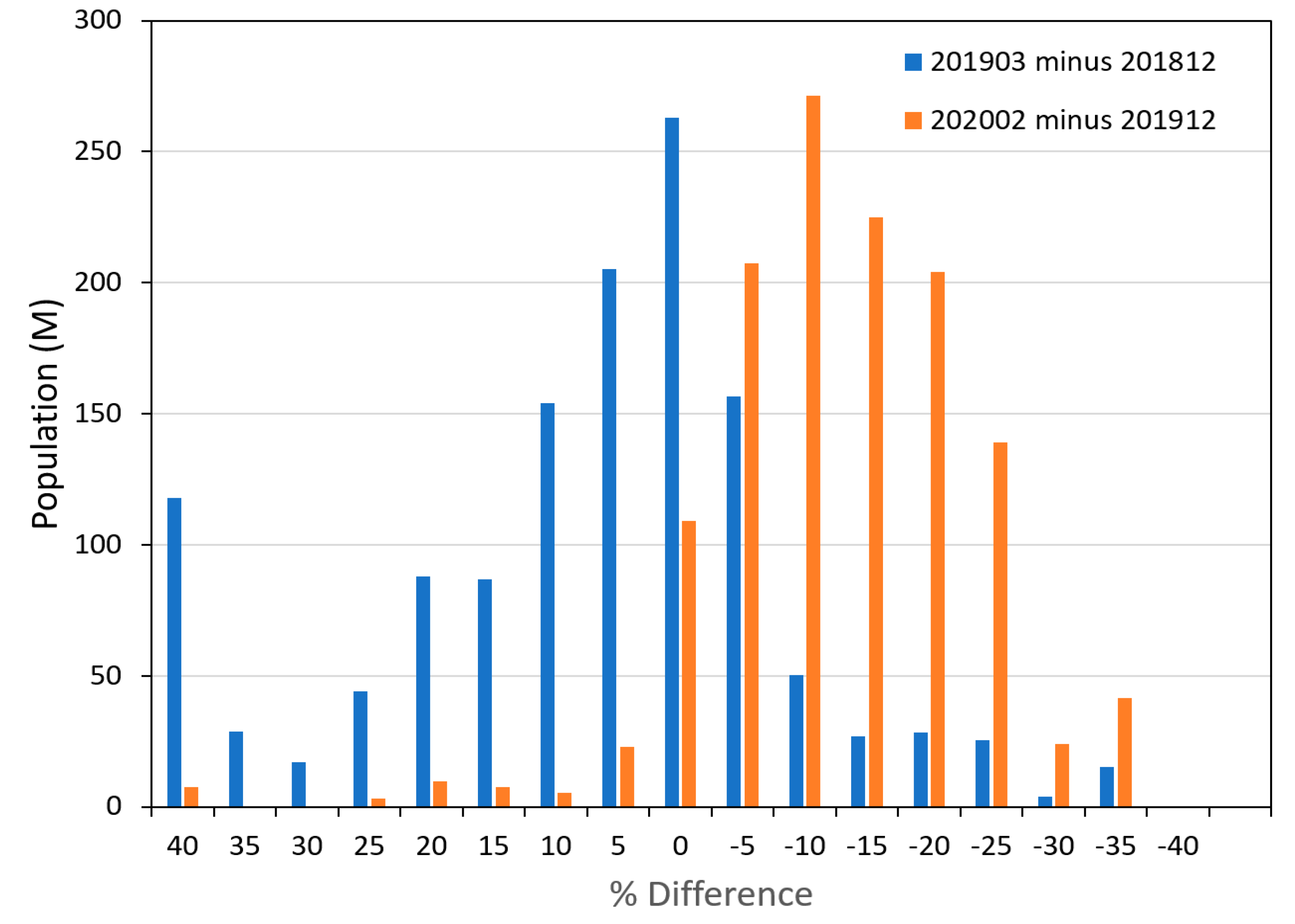
Histograms of percent differences versus population:Figure 9 shows population tallies versus percent difference in brightness for the two pairs of months. In the pre-pandemic reference set, 61% of the population was located in administrative units, where the brightness of lighting increased. In contrast, 82% of China’s population lived in administrative units in February 2020, where the brightness of lighting decreased.
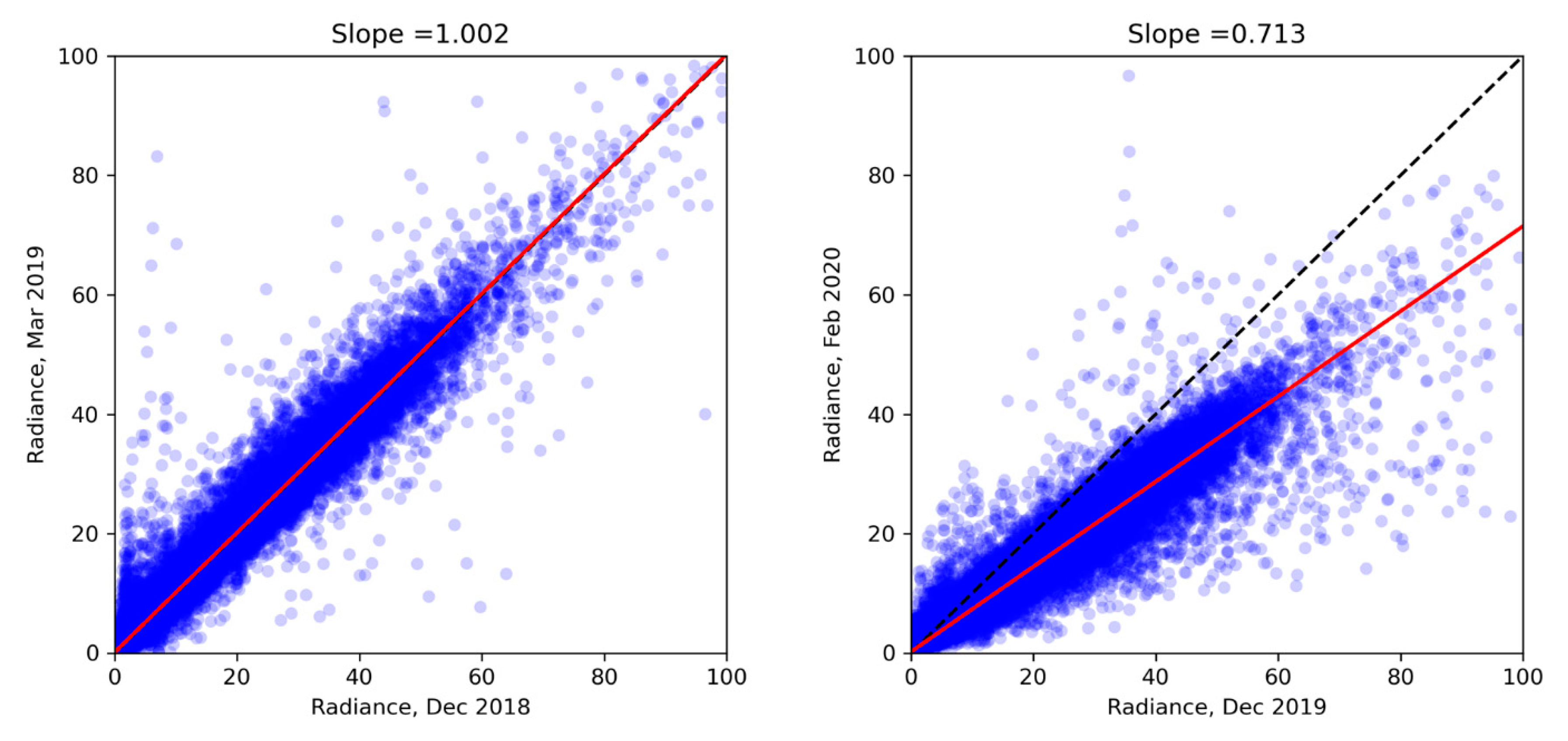
Beijing scattergrams: Another way to see the magnitude of the dimming was using the comparison between pre-pandemic and pandemic scattergrams.
Figure 10 shows scattergrams made with all of the grid cells in Beijing. The pre-pandemic scattergram was on the left, and the pandemic scattergram was on the right. In both cases, December is on the X axis. The slope of the regression line for December 2018 and March 2019 was 1.002, indicating no significant change in radiance levels between these two months. The slope dropped to 0.713 in the pandemic scattergram due to substantial dimming in February 2020.
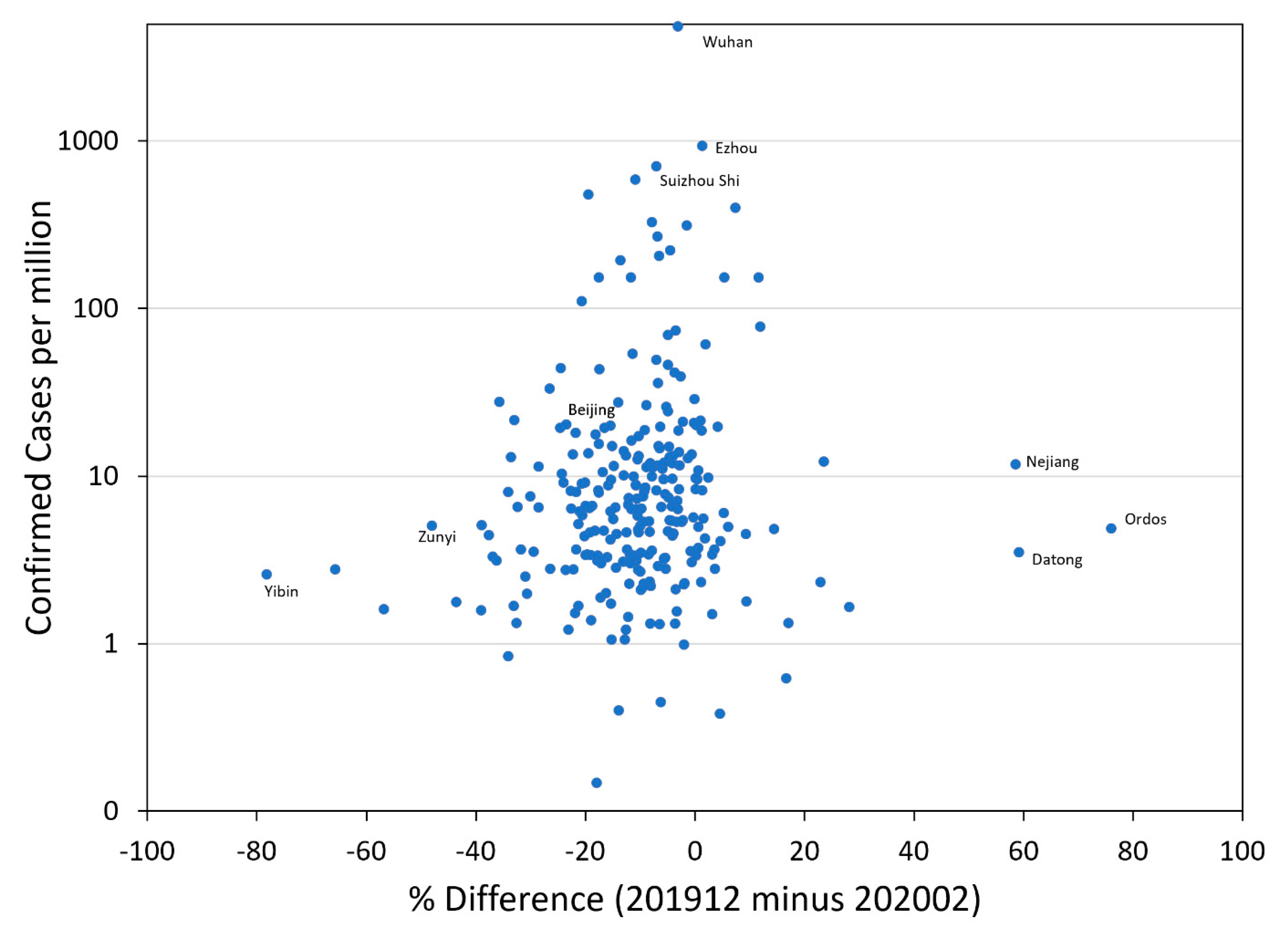
Correlation with confirmed cases: The percent change in SOL from the pandemic monthly pair was matched to the number of confirmed COVD-19 cases per million people from January 15 to the end of February 2020 [
13]. The results (
Figure 11) indicated that dimming occurred in many cities with few confirmed cases.
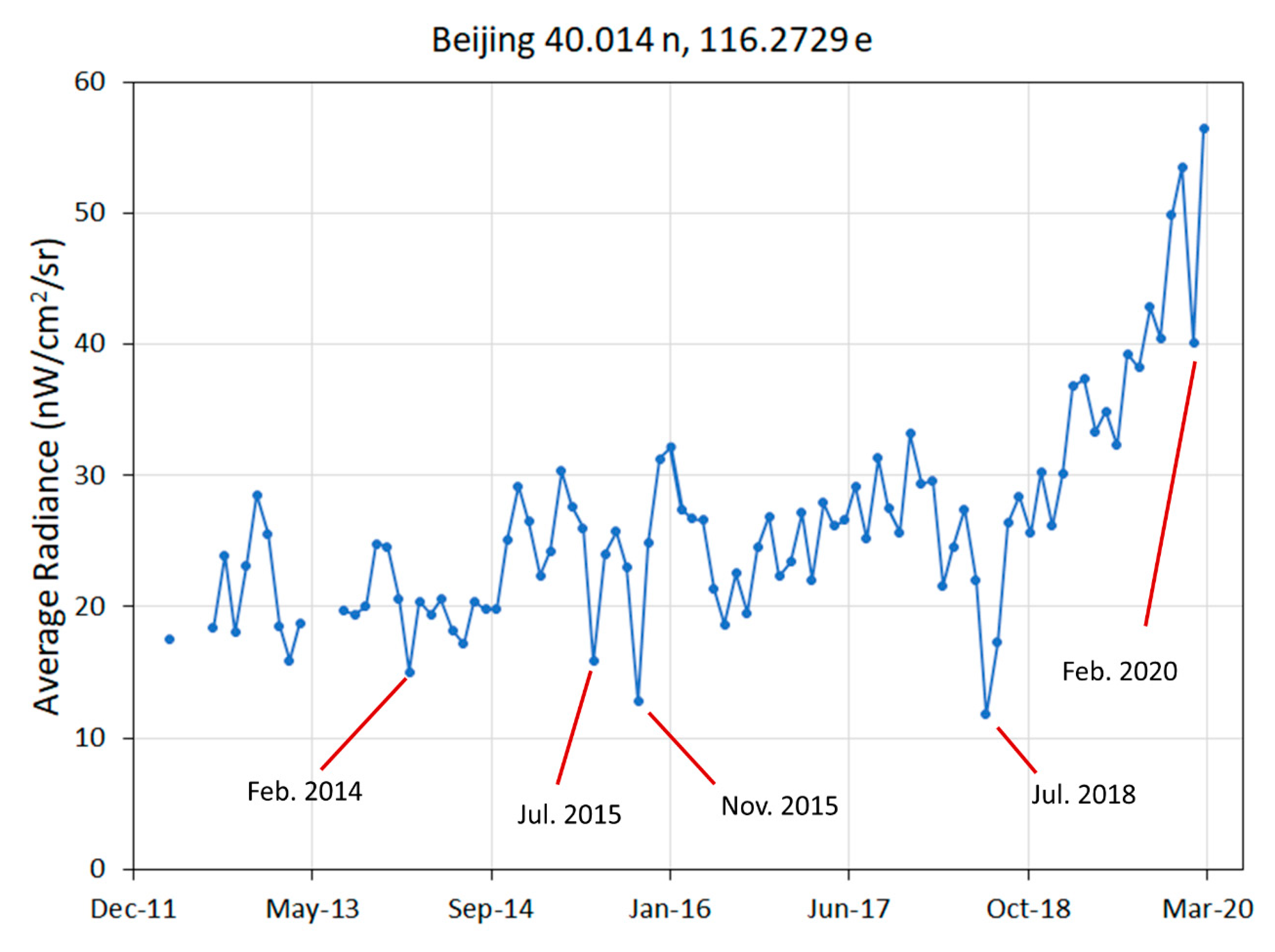
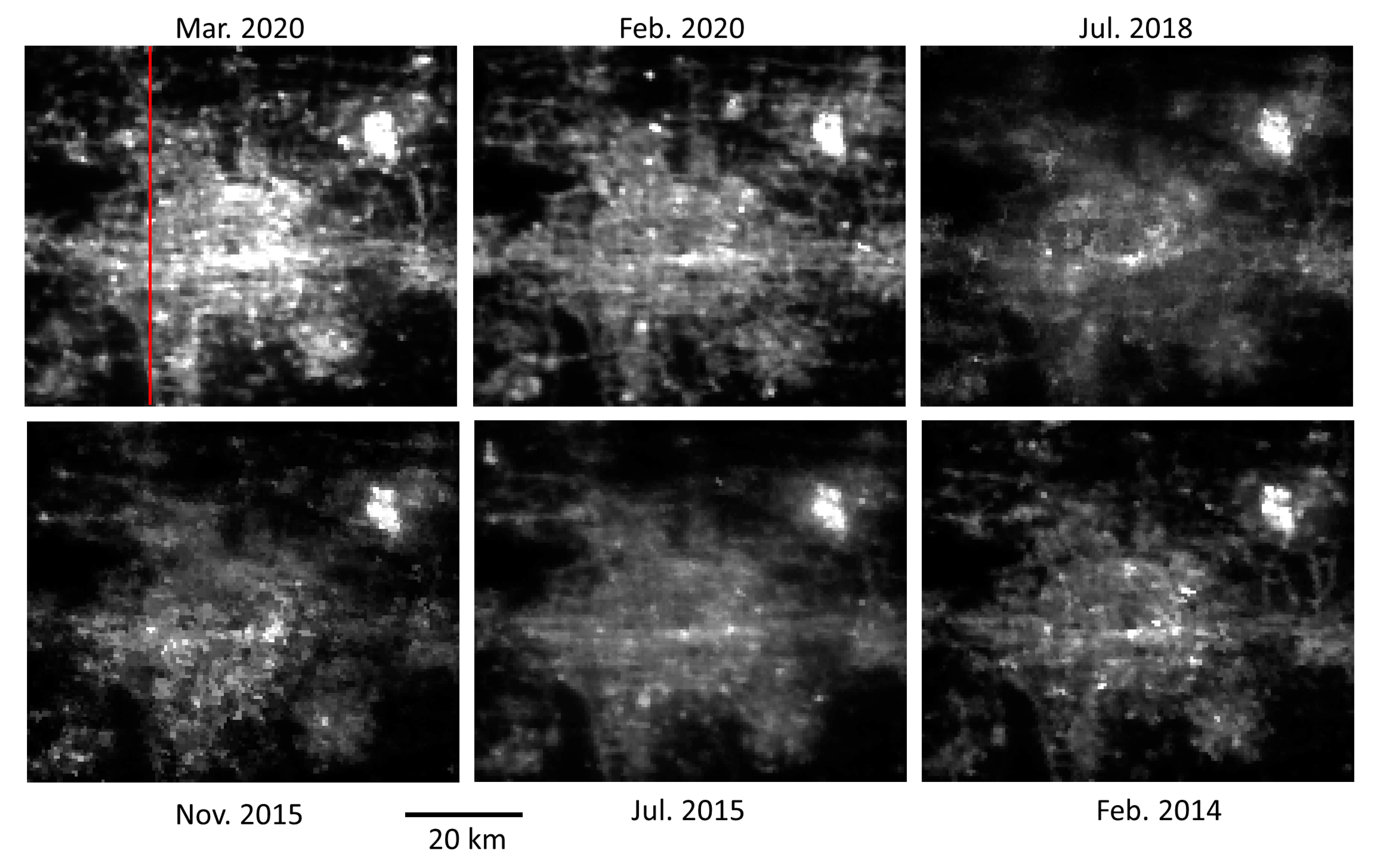
Is the February 2020 dimming unique? To examine whether the February 2020 dimming is unique, we constructed a data cube with 96 monthly cloud-free composites of Beijing, spanning from April 2012 to March 2020. In examining the monthly temporal profiles for individual grid cells, it was possible to see a radiance dip in February 2020 relative to those in the previous two months and March 2020 (
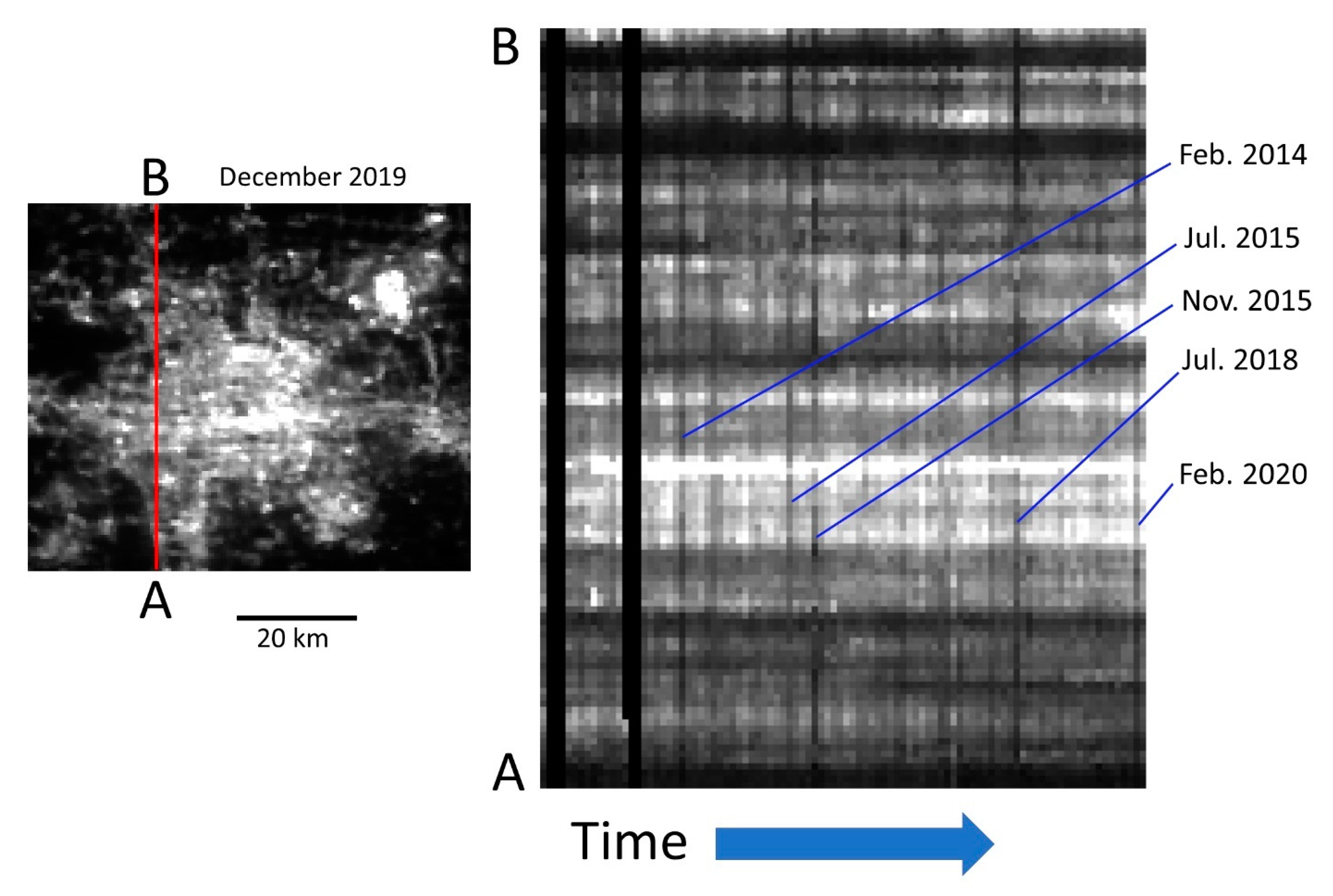
Figure 12). However, there were other dips along the profiles in magnitude comparable to that in February 2020. To determine if the additional dimming events were isolated geographically or spatially extensive, we constructed a temporal slice along a north-south transect across the data cube (
Figure 13). Spatially extensive dimming showed up as dark vertical lines. There were two black vertical lines during the early part of the record and three month-wide data gaps centered on the summer solstice caused by the exclusion of stray light contamination prior to the advent of the “stray light correction” [
17]. However, there were additional dark vertical lines indicating widescale dimming of lights. Regardless of where the transect was taken, the same set of months appeared as dark vertical lines. The most prominent of these were February 2014, July and November 2015, July 2018, and February 2020. December 2019 was bright with sharply defined features (
Figure 14). To investigate the cause of the dimming, average radiance images in each of these months were compared to that in December 2019 (
Figure 14). The December 2019 contrast enhancement was applied to each of the other monthly images. It can be seen that December 2019 has the brightest features and the details were sharp. The February 2020 geographic feature details were comparable to those in December 2019, but the radiance levels were dimmed. The other months exhibited dimming with the blurring of spatial details. The examination of the cloud-free coverages revealed that the pre-pandemic dimmed months were short with cloud-free coverages and had multiple data gaps with zero cloud-free coverages (
Figure 15).
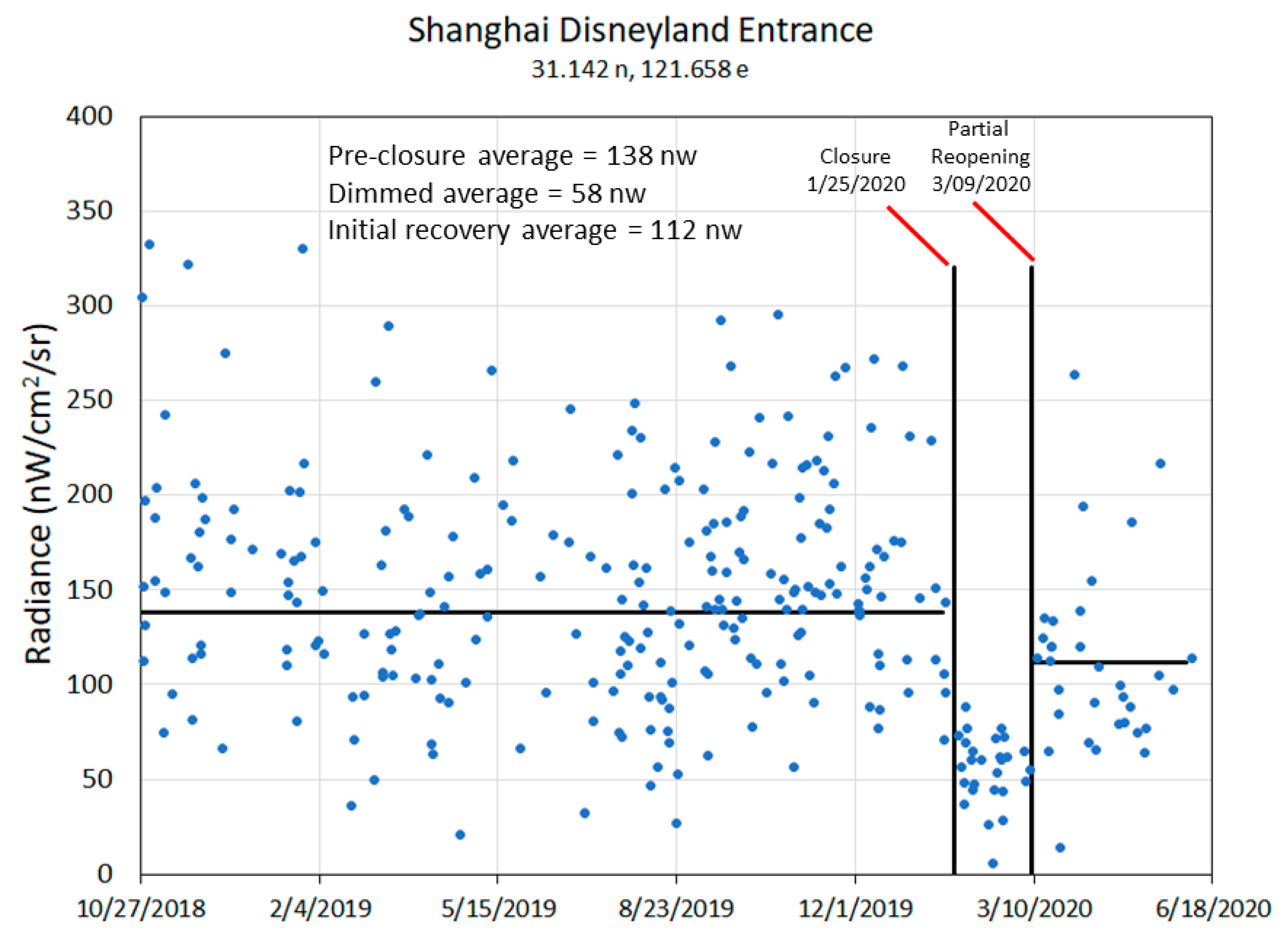
Examination of dimming and recovery with a nightly temporal profile: One of the grid cells with the sharpest decline in lighting during February 2020 covered the entrance to Shanghai Disneyland. The site closed on 25 January 2020 and partially reopened on 9 March 2020 [
18]. A nightly temporal profile of the entrance is shown in
Figure 16, only filtered to remove cloud observations. The start dates of dimming and recovery exactly matched the reported closure dates. The dimmed state was 42% of the pre-closure radiance level. However, the recovery state brightness through 6 June 2020 was 81% of the pre-closure level.
4. Discussion
The decline in the brightness of lighting in China during the COVID-19 lockdown was in the 3–24% range and was observed in four different ways. The simplest way to see the dimming was by comparing radiance difference images for two selected pairs of monthly composite images, matching seasonally and avoiding the Chinese New Year. We used the brightness in December 2018 minus the brightness in March 2019 as the pre-pandemic pair (reference set) and the brightness in December 2019 minus the brightness in February 2020 as the pair impacted by the lockdown (pandemic set). The reference and pandemic difference images were density-sliced to enhance the visual interpretation of dimming and brightening. Major cities in China readily showed dimming in the difference images.
Another way to see the dimming is by using full province SOL tallies for more than 344 level 2 administrative units. The difference between the reference and pandemic set tallies made it possible to see the prevalence of dimming in February 2020. We conducted a t-test of unequal variances to ascertain whether the difference of the mean between the pre-pandemic and pandemic pair was significant or not. The t-test of unequal variances at a 0.05 significance level was associated with a significant effect t (649) of −9.60 and
p of 1.77 × 10
−20. Thus, the pandemic difference pair had a larger statistically significant mean than the pre-pandemic pair (
Table 2).
Radiance scattergrams offer another way to visualize the dimming. In the reference set, the scattergram data cloud was aligned with the diagonal, indicating no systematic dimming or brightening between the two months of the reference set. In contrast, the scattergram of the pandemic set shows the entire data cloud shifted to lower radiance levels in February 2020 relative to in December 2019.
The fourth approach used to see the dimming is with nightly temporal profiles. Here, it was possible to see the precise date when dimming started, the radiance level of the lighting during the dimming period, the date range of recovery, and the recovery level.
An important aspect of this study is the filtering to exclude grid cells impacted by snow cover, low numbers of cloud-free coverages, and background areas, where lighting was detected.
5. Conclusions
During the first half of 2020, nearly the entire population of the world lived under some form of human contact restrictions aimed at reducing the transmission of COVID-19. The restrictions in China began with a lockdown in Wuhan on 24 January 2020, and these were quickly extended across China. The lockdown featured the closures of schools, restaurants, travel, and many factories and commercial centers. People were required to stay at home. The associated economic impacts are significant and are still being tallied.
China’s lighting and electricity demand have long been on an upward trajectory, tracking the expansion in construction and economic activity levels. This pattern went in reverse during the COVID-19 lockdown, resulting in dramatic declines in the brightness of electric lighting observed by satellite. The declines can be seen clearly in multiple cities with the difference image calculated by the brightness in December 2019 minus the brightness in February 2020. While brightness declines were prevalent, it was common to find patches with lighting increase mixed with the areas having decline. The situation was reversed in the pre-pandemic difference images, where brightening prevailed amid a patchwork pattern of dimming and brightening. The brightness decline in February 2020 lighting levels can also be seen in scattergrams formed with the December 2019 radiances.
With nightly DNB radiance profiles, it is possible to identify the start dates of dimming and recovery, plus the recovery level relative to the pre-pandemic condition. This was demonstrated for the grid cell containing the Shanghai Disneyland entrance. This site was chosen, because it is one of a few facilities having precise closure and partial reopening dates published. The dimming and onset dates of recovery observed by VIIRS exactly matched the closure and reopening dates. The level of lighting recovery following the reopening was 81% of the pre-pandemic lighting level.
In exploring the DNB monthly composite time series, we found several issues that other researchers should be aware of. First, the background radiance levels varied both spatially and temporally. If the focus of an analysis is electric lighting, it is important to zero out the background using a radiance threshold. In nearly every monthly composite, there were data gaps, where zero cloud-free observations were available. These should be excluded from multitemporal analyses in a way to avoid corrupting change detection results. Snow cover resulted in increased brightness of light, which can also lead to erroneous conclusions on brightness changes. Finally, we found the evidence that there were cases, where undetected clouds resulted in the blurring and dimming of lighting features. This suggested that a lighting sharpness index could be used in conjunction with cloud detections to improve both the annual and monthly DNB composites.
This study confirms that satellites are able to detect the dimming of lighting associated with the current pandemic lockdowns. We found no correlation between the percent dimming in February 2020 and COVID-19 confirmed case numbers. This suggested that the dimming of lights was primarily associated with “stay-at-home” lockdowns designed to slow the virus transmission. It is possible that the recovery pattern of lighting can be used as an indicator of the economic recovery. Disaster and conflict lighting outages are typically due to damage to generation or distribution systems. In the case of COVID-19, the power generation and distribution systems remain intact. Therefore, in theory, if the lights dim, they could return to normal shortly after government lockdowns are lifted. If the lighting fails to return to pre-lockdown levels, this is an indication that the economic damage continues to affect lighting. The results from this study indicate that the dimming and recovery of lights can be effectively monitored from space and that recovery levels can be rated relative to pre-pandemic radiance levels.

 ,
, 


