Article

Novel Machine Learning Approaches for Modelling the Gully Erosion Susceptibility

1
Department of Geomorphology, Tarbiat Modares University, Tehran 14117-13116, Iran
2
Department of Watershed Management, Gorgan University of Agricultural Sciences and Natural Resources (GUASNR), Gorgan 3184761174, Iran
3
Department of Geography, The University of Burdwan, West Bengal 713104, India
4
Geoscience Platform Research Division, Korea Institute of Geoscience and Mineral Resources (KIGAM), 124 Gwahak-ro Yuseong-gu, Daejeon 34132, Korea
5
Department of Geophysical Exploration, Korea University of Science and Technology, 217 Gajeong-ro Yuseong-gu, Daejeon 34113, Korea
6
Centre for Advanced Modelling and Geospatial Information Systems (CAMGIS), Faculty of Engineering and Information Technology, University of Technology Sydney, Ultimo, NSW 2007, Australia
7
Department of Energy and Mineral Resources Engineering, Sejong University, Choongmu-gwan, 209 Neungdong-ro, Gwangjin-gu, Seoul 05006, Korea
8
Center of Excellence for Climate Change Research, King Abdulaziz University, P.O. Box 80234, Jeddah 21589, Saudi Arabia
9
Earth Observation Center, Institute of Climate Change, Universiti Kebangsaan Malaysia, Bangi 43600 UKM, Selangor, Malaysia
10
Institute of Research and Development, Duy Tan University, Da Nang 550000, Vietnam
*
Author to whom correspondence should be addressed.
Remote Sens. 2020, 12(17), 2833; https://doi.org/10.3390/rs12172833
Submission received: 6 July 2020 / Revised: 22 August 2020 / Accepted: 25 August 2020 / Published: 1 September 2020

Abstract

:
The extreme form of land degradation caused by the formation of gullies is a major challenge for the sustainability of land resources. This problem is more vulnerable in the arid and semi-arid environment and associated damage to agriculture and allied economic activities. Appropriate modeling of such erosion is therefore needed with optimum accuracy for estimating vulnerable regions and taking appropriate initiatives. The Golestan Dam has faced an acute problem of gully erosion over the last decade and has adversely affected society. Here, the artificial neural network (ANN), general linear model (GLM), maximum entropy (MaxEnt), and support vector machine (SVM) machine learning algorithm with 90/10, 80/20, 70/30, 60/40, and 50/50 random partitioning of training and validation samples was selected purposively for estimating the gully erosion susceptibility. The main objective of this work was to predict the susceptible zone with the maximum possible accuracy. For this purpose, random partitioning approaches were implemented. For this purpose, 20 gully erosion conditioning factors were considered for predicting the susceptible areas by considering the multi-collinearity test. The variance inflation factor (VIF) and tolerance (TOL) limit were considered for multi-collinearity assessment for reducing the error of the models and increase the efficiency of the outcome. The ANN with 50/50 random partitioning of the sample is the most optimal model in this analysis. The area under curve (AUC) values of receiver operating characteristics (ROC) in ANN (50/50) for the training and validation data are 0.918 and 0.868, respectively. The importance of the causative factors was estimated with the help of the Jackknife test, which reveals that the most important factor is the topography position index (TPI). Apart from this, the prioritization of all predicted models was estimated taking into account the training and validation data set, which should help future researchers to select models from this perspective. This type of outcome should help planners and local stakeholders to implement appropriate land and water conservation measures.

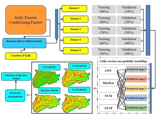
Graphical Abstract

1. Introduction

In the last few decades, modern societies have witnessed various types of degradation of natural resources; above all, soil and water have become more prominent [1]. Land degradation through water-induced soil erosion is the most critical threat to human life and a number of environmental problems are occurring, particularly in the arid and semi-arid region of Iran [2]. Soil erosion is not only an extreme form of land degradation; it is also responsible for a gradual decline in agricultural productivity [3,4,5]. The formation of soil is a natural process, although the net loss of soil is much higher than the formation of regolith due to the gradual degradation of this resource and the influence of anthropogenic activities [6,7]. It has been estimated that almost 6 million hectares of fertile land are lost annually on a global scale due to soil erosion [8]. In the case of Iran, it is approximately 2 to 2.5 billion tons per year and ranks second in the world in terms of soil erosion [9]. In Iran, therefore, the rate of soil erosion is occurring at an alarming rate, making it a national threat [10]. This enormous amount of soil erosion is mainly due to arid and semi-arid climatic conditions and more than 75% of the area is exposed to water-induced soil erosion, i.e., erosion in the form of gullies [10]. More specifically, there is a long dry season with a short wet season, which influences extreme rainfall and causes maximum surface runoff over infiltration [10]. It has also been reported that Iran is facing several intimidating gully incisions around the world [11,12]. Various types of environmental problems, such as desertification, sedimentation in rivers, as well as reservoirs, floods, and soil fertility losses have occurred due to the severe impact of gully erosion [13,14]. In recent times, due to its large impact on environmental degradation and national economic losses, the threat of gully erosion has been taken into account in an appropriate manner. Therefore, in order to understand the mechanism of water-induced gully erosion and to overcome this problem in an optimal way, gully erosion susceptibility mapping (GESM) is a key strategy and must be considered as an initial task. The GESM is derived from the relationship between different geo-environmental conditioning factors and occurrences of gullies [15].
Gully erosion is water-induced soil erosion and is one of the most destructive forms of soil erosion in the world [16,17]. A gully can be defined as a permanent vertical deep channel with a temporary flow of water; the depth varies from 30 cm to several meters and sometimes it is several hundred meters long [18,19,20]. Apart from this, the existence of one type of gully is limited during the wet season, which is called the ephemeral gully. Gully erosion is a very complicated process and it correlates with many factors, such as topography, soil characteristics, lithology, rainfall, land use, and the nature of vegetation [21,22,23]. Running surface water is responsible for the initiation and development of gullies by removing soil particles and ultimately transporting them in the downslope direction [24]. Primarily, two types of approaches have been recognized to evaluate the occurrences of gully erosion [25,26,27]. First, using a regression analysis, we explored the relationship between the occurrence of gully erosion and the topographical condition. Second, gully erosion response curves were prepared using machine learning techniques [28]. The predictive regression approach is considered to estimate and identify the conditioning relation among variables. Regression solutions estimated using various principles (e.g., optimization, minimal square, etc.) are not inherently similar [29]. Machine learning may analyze vast quantities of data and identify complex changes and nature that would not be obvious to individuals. This algorithm is well suited for resolving multi-dimensional and multi-variety information, and can do so in complex or unpredictable situations. As this algorithm learns its skills, it continues to develop in terms of accuracy and performance. Machine learning needs the training of large volumes of data, which should have been inclusive/true and of an excellent standard. There may also be occasions when they wait to produce additional knowledge. ML requires ample time to let algorithms learn and improve sufficiently to perform their tasks with reasonable precision and relevance. It also requires huge sources for it to operate. This might mean extra computing power needs for analysis. Another major obstacle is the ability to analyze the algorithm-generated output precisely.
Over the last few decades, with the arrival of remote sensing (RS), geographic information system (GIS), and various statistical approaches, susceptible areas have been identified in various fields, such as gully erosion [30], landslide [31], groundwater potential zone [32], etc. Basically, there are three types of susceptibility mapping based on multi-criteria decision analysis (MCDA), statistical analysis, and more recently the widely used machine learning algorithm. Extensive literature surveys show that different types of models have been used throughout the world over time to map the susceptibility of gully erosion. It is indeed necessary to remember that the MCDA models presume that the improvement of the attribute does not influence the preferences of the different criteria. This feature, recognized by the technical resource of reciprocal preferred autonomy, is related to the particular question, and the nature of the research [33]. Experts must always determine if autonomy is an expectation for fields and, if not, recommend quite complicated MCDA (multi-criteria decision analysis) systems that integrate relationships [34]. Most importantly, knowledge-based MCDA [11] and statistical analysis based on continuous, binary, and categorical data, such as the information value [23,35], conditional probability [36], certainty factor [37], frequency ratio [38], evidential belief function [2], index of entropy (IoE) [39], weights of evidence (WoE) [40], and logistic regression [2,41], has been widely used by several researchers. In the case of the machine learning algorithm, the most successful models for GESM are the multi-layer perception approach (MLPC) [42], multivariate adaptive regression spline (MARS) [39], artificial neural network (ANN) [43], classification and regression trees (CART) [23], maximum entropy (ME) [44], decision tree (DT) [45], boosted regression tree [15], stochastic gradient treeboost (SGT) [46], random forest (RF) [47], bagging best-first decision tree [48], general linear model (GLM) [49], maximum entropy [50], etc. In general, GESM with machine learning models is more proficient at predicting susceptible areas than statistical analysis. Simulation focuses, in a number of ways, on the related mechanism used, including machine learning or deep learning. Computational products are formulated to predict missing parameters, objects, or events, as their name implies. They sometimes rely on grouping, convergence, and object image processing algorithms [51].
In the current study, semi-humid, semi-arid, and Mediterranean climate types in the province of Golestan, Iran were chosen to map the susceptibility of gully erosion due to its serious damage and the major environmental problems caused by gully erosion. Therefore, the causes of extensive gully erosion, their development, and susceptibility mapping for management and planning purposes must be identified. Therefore, the objectives of our current research work were to identify the most reliable maps of gully erosion susceptibility and to recognize the main conditioning factors responsible for their development. Therefore, in order to meet our objectives, a maximum entropy (MaxEnt), artificial neural network (ANN), support vector machine (SVM), and general linear model (GLM) machine learning algorithm with 90/10, 80/20, 70/30, 60/40, and 50/50 random partitioning of training and validation samples were selected for the purpose of estimating the susceptible part of gully erosion. The selection of the machine learning models for gully erosion susceptibility mapping was based on the previous literature in this region as well as the same climatic conditions [39,43,52,53,54]. The optimal models suggested by the various researchers were considered for the estimation of gully erosion susceptibility. In previous studies, researchers have attempted to increase the accuracy of the model by considering ensemble approaches rather than a single model. In this perspective, this kind of approach was avoided in order to avoid the problem of over-fitting. Apart from this, the study considered the modification of existing models by considering the random partition of samples. The final result of different GESM models was validated through the area under receiver operating characteristic curve (AUROC). In addition, the jackknife test was used to give different GECFs importance regarding the susceptibility to gullies. This type of machine learning algorithm is not only capable of estimating susceptibility with adequate accuracy but is also capable of handling the large amount of data of the predicted models. Supervised ML approaches usually involve partitioning information into multiple parts for clustering algorithm training, validation, and final testing. Training and validation are usually performed on a test set to discover the perfect variables for a classification model. It was accompanied by the implementation of a classification algorithm for a different test sample with optimal factors for estimating the generalization efficiency of the classification model. For minimal data, this differentiation of the test dataset results in a difficult trade-off among several predictive significances in the classifier output estimation against improved simulation analysis and significant optimal fitting. Apart from the models, the optimum separation capacity of the samples in the appropriate manure may increase the efficiency of the models without compromising the importance of the classifier. In terms of uniqueness, this study is capable of estimating the importance of sample partitioning approaches to improve model performance and to reduce predictive bias. This approach is used for the first time in gully erosion susceptibility modeling, taking into account the optimal capacity of the model. Finally, GES maps will provide appropriate strategies for restoration in the various sectors, i.e., agriculture, land use, and watershed management planners, in a sustainable manner.

2. Materials and Methods

2.1. Study Area

The study area occupies an area of 790 km2 and lies between 37°30′00″ to 37°50′00″ N, and 55°31′40″ to 56°2′10″ E in the northeast part of Golestan province. Elevation ranges between 160 and 1490 mt. mean sea level (MSL) (Figure 1). More than half of the basin has mountainous morphology with gentle slopes and is a part of the Alborz Mountains. The slope angle at steep slopes reaches up to 118%. The average annual rainfall varies from 346 to 610 mm, with the maximum rainfall conducted in southern parts. The minimum and maximum temperatures are 8 and 16 °C. Three main climatic characteristics of semi-humid, semi-arid, and Mediterranean are evident in the study area. Agriculture, as the predominant land cover, is conducted in most of the study area (i.e., 45.35%), followed by rangelands (38.07%), forests (15.95%), and residential areas (0.64%) (Table 1). Geologically, the largest portion of the region corresponds to the grey to black shale and thin layers of siltstone and sandstone (73.94%), followed by Ammonite bearing shale with the interaction of limestone (12.48%), grey thick-bedded limestone, and dolomite (6.26%), and the remaining area is dominated by other formations described in detail in Table 2.

2.2. Methodology

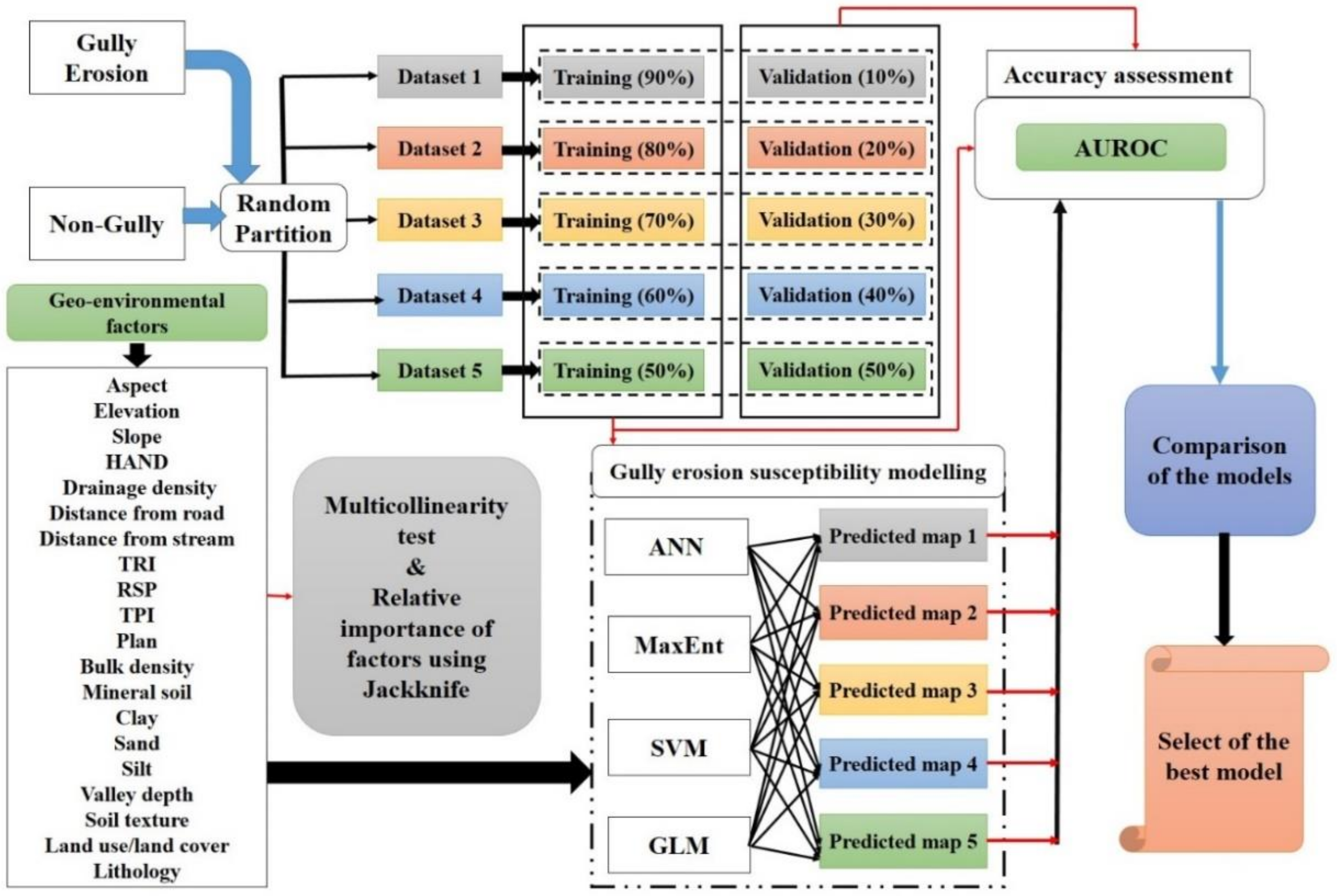
The present study followed several steps as follows:
(i)
The gully erosion inventory map and gully erosion causality factors preparations: In the current study, a total of 1115 gully head cut locations were identified using the high-resolution images, field investigation, global positioning system (GPS), and a number of gullies were received from Natural Resources and Watershed Management Organization of the Golestan Province. The 20 environmental factors were considered for the modeling purpose.
(ii)
Multi-collinearity analysis among the gully erosion factors using the variance inflation factor (VIF) and tolerance limit was done using SPSS software.
(iii)
The significance and effectiveness of factors was carried out using the MaxEnt model (Jackknife test).
(iv)
GES maps were prepared using the MaxEnt, ANN, SVM, and GLM models.
(v)
The GESM model’s performance was validated through the area under receiver operating characteristic curve (AUROC).
The detailed methodology for estimating the susceptibility of gully erosion in the light of these novel approaches is shown in Figure 2.

2.3. Gully Inventory Map

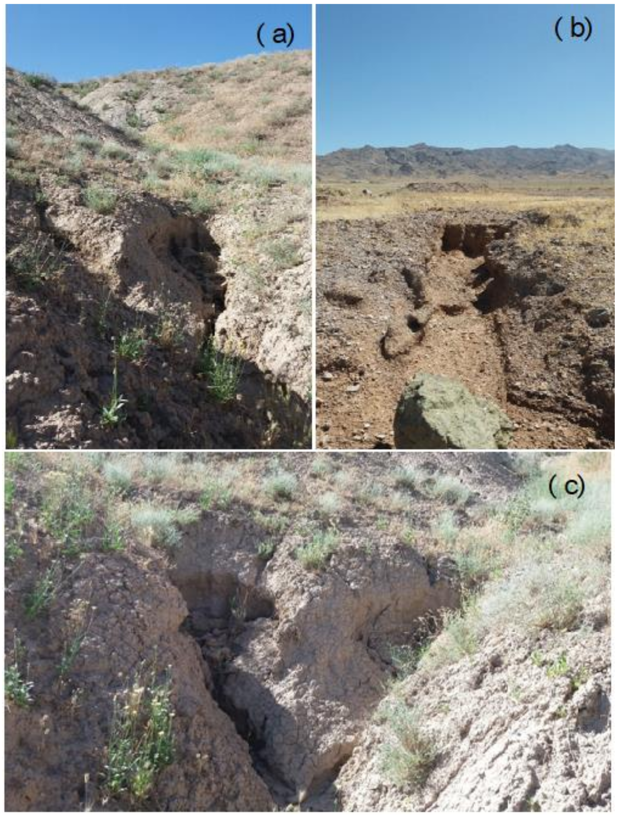
The gully erosion inventory map (GEIM) is the basic tool for creating the GESMs. GEIM shows the spatial distribution of gullies and geometry. Through the historical and present gully distributions, one can predict the future risk of the gully erosion of the area. In the present study, the RS and GIS techniques were applied to generate the GEIM. The geographical location of gullies was partially acquired from the archived data of Natural Resources and Watershed Management Organization of the Golestan Province (NRWMOGP). Further, extensive field surveys were conducted supported by geoinformatics (Google Earth images and a handheld GPS device), through which the previous gully inventory map was amended, and an all-inclusive map was generated in ArcGIS 10.3. The produced inventory map was then randomly split into two sets of training and validation data in five replicates, each of which possessed a different training:validation balance. The balance values commenced in favor of the training dataset as it held 90% of the gullies while the remaining was cast-off for further validation, and perpetually more samples were transmitted to the validation dataset. As such, five training:validation samples of 90:10%, 80:20%, 70:30%, 60:40%, and 50:50% were considered to investigate how the dataset’s transient distribution can influence models’ performances. Some major erosion-prone areas are shown in Figure 3, due to the nature and vulnerability of the erosion that we can easily understand.

2.4. Data Preparation

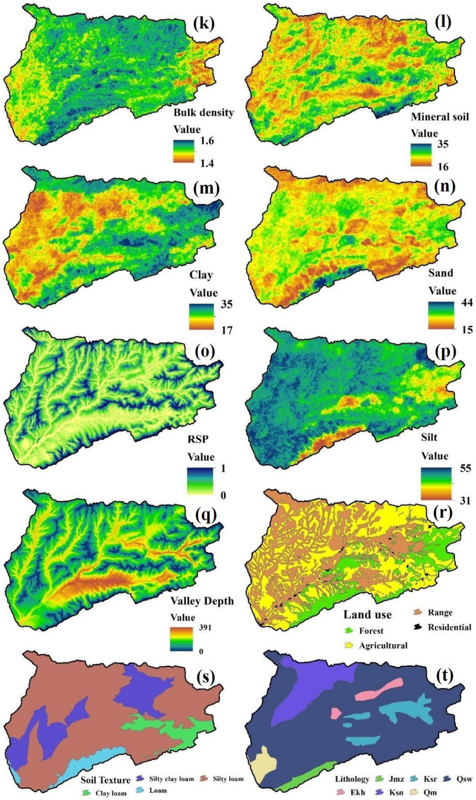
Different geo-environmental factors, such as topographic, hydrological, geological, soil, and environmental factors, are important parameters for GESM (gully erosion susceptibility mapping) (Table 3). It is also an important step in the selection of the various appropriate geo-environmental factors for the preparation of GESM using different machine learning models [15]. In this study, based on a previous literature review [10,23,55], the availability of data, extensive field survey, and multi-collinearity analysis, we selected 20 GECFs, namely the topography position index (TPI) [56], plan curvature [57], elevation, aspect [58], slope [58], height above nearest drainage (HAND) [59], drainage density [60], distance from stream [61], terrain ruggedness index (TRI) [42], distance from road [62], bulk density [63], mineral soil, clay content, sand content, relative slope position (RSP) [64], silt content, valley depth, land use, soil texture, and lithology (Figure 4a–t).
All these factors were derived from different sources. The Advanced Land Observing Satellite (ALOS) digital elevation model (DEM) 12.5 m resolution data were downloaded from the Alaska Satellite Facility (ASF) for the extraction of topographic and hydrological factors, such as the topography position index (TPI), plan curvature, elevation, aspect, slope, drainage density, distance from stream, terrain ruggedness index (TRI), and relative slope position (RSP). The geological map was collected from Geological Society of Iran (GSI) (http://www.gsi.ir/) at a scale of 1:100,000 to generate the lithology map. The topographic map was acquired from National Geographic Organization of Iran (www.ngo-org.ir) at a scale of 1:1:50,000 along with Google Earth images and Landsat 8 satellite images, which were also used to produce land use and roads network maps.
Topography position index (TPI):
More specifically, TPI is used to measure topographic slope positions. TPI is the measure of differences between the elevation at the central point and the average elevation around it [65]. The following equations were used to estimate the TPI. The TPI map is shown in Figure 4a and the value ranges from −38.8 to 54.8:
T P I = E P i x e l E S u r r o u n d i n g ,
where E P i x e l is the elevation at the central point and E S u r r o u n d i n g is the average elevation of the neighboring areas.
Plan curvature:
Plan curvature signifies the overland flow of water in terms of its diverging and converging, and plays an important factor in gully erosion studies [35]. The value of plan curvature ranges from −6.1 to 9.1 (Figure 4b).
Elevation:
Elevation influences the rainfall and related runoff process, which is largely employed in geo-hazard modelling like GESM [66]. The elevation of this region ranges from 160 to 1490 m (Figure 4c).
Slope aspect:
Solar radiation, vegetation covers, and evapo-transpiration largely depend on the slope aspect [67], which is considered to be one of the major parameters for geo-hazard susceptibility mapping. The aspect map of this study area is shown in Figure 4d.
Slope:
Slope angle largely affects the surface runoff, infiltration, pattern of drainage density, and soil erosion [35,68]. Therefore, slope angle has always been used as one of the major factors for mapping GESM. In this region, the angle of slope varies from 0% to 118% (Figure 4e).
Height above nearest drainage (HAND):
The HAND model emphasizes the relative heights beside the drainage network and influences the soil gravitational potential [59]. HAND is calculated by using the DEM and DEM flow field in a GIS environment [69]. The value of the HAND map ranges from 0 to 494 (Figure 4e).
Drainage density:
Drainage density has a major influence on erosion in the form of the initiation and development of rills gullies, etc. a higher drainage density has a minimum infiltration rate and higher runoff capacity, and vice versa [66]. Drainage density was calculated by using the following equation [70]. The value of drainage density ranges between 0 and 3.32 km/km2 (Figure 4f):
D D = i = 1 n S i a ,
where i = 1 n S i indicates the total length of all drainages in km and ‘a’ is the total area of the drainage basin in km2.
Distance from stream:
Gullies are primarily associated with the drainage system, and there is a significant positive relationship between the distance from the stream and the occurrence of gullies [71]. The distance from the stream map is shown in Figure 4g and the range varies from 0 to 1959 m.
Terrain ruggedness index (TRI):
The concavity and convexity of an area is indicated by TRI, which also influences gully erosion occurrences [72]. Apart from this, different pedo-geomorphic processes can directly influence the amount of TRI in a specific geomorphic region. The following equation was used to calculate TRI. The value of TRI ranges between 0 and 37 (Figure 4h):
T R I = X ( m a x 2 m i n 2 ) ,
where X represents the altitude of every neighbor cell to a definite cell, and max and min are the highest and smallest altitude among different neighboring cells.
Distance from road:
The distance from the road is another important parameter for the gully erosion and the preparation of the GESM. Due to the construction of the road, the stress and strain of the slope can be increased and as a result, there were disturbances and failures of the slope [62]. The distance from the road map is shown in Figure 4i and the value ranges from 0 to 4532 m.
Bulk density:
Bulk density is defined as the mass per unit volume of the loose powder bed [63]. Bulk density was estimated by using the following equation. The range of the bulk density in this region varies from 1.4 to 1.6 g/mm in the study area (Figure 4j):
B D = M V o ,
where M represents the mass in grams and V o indicates the untapped apparent volume in milliliters.
Mineral soil, clay content, and sand content:
The value of mineral soil, clay, and sand varies from 16 to 35, 17 to 35, and 15 to 44, respectively (Figure 4k–m).
Relative slope position (RSP):
RSP helps to understand the various topographical characteristics, such as flat surface, valley, ridge-top, foot-slope, mid-slope, and upper slope [73]. The value of the RSP map for the current study area varies from o to 1 (Figure 4n).
Silt content and valley depth:
Silt content and valley depth are also important factors for GESM. In the present study, the silt content and valley depth varies from 31 to 55 and 0 to 391, respectively (Figure 4o,p).
Land use:
The formation of gullies and associated land degradation depends to a large extent on land use. The land use map of the area was prepared using the maximum likelihood algorithm of the supervised classification technique [74]. Table 2 shows different land use types and their geographical areas, i.e., forest, agricultural land, range, and residential areas (Figure 4q).
Soil texture and lithology:
Soil texture in this study area has been categorized into four types namely clay loam, salty clay loam, loam, and silty loam (Figure 4r). The land surface process of the area is highly influenced by lithological characteristics and one of the most significant factors for large-scale erosion, such as the creation and development of gullies [35,75]. In this study, six types of lithological units were found (Figure 4s) and their description is given in Table 2.

2.5. Multi-Collinearity Assessment

Multi-collinearity analysis can be defined as the relationship between two or more variables in the data set and the linear relationship among variables [2]. Generally, various geo-environmental conditioning factors have been used to prepare GESM. Thus, multi-collinearity analysis was therefore used to identify the perfect relationship between the variables. Multi-collinearity occurs when there is a very high correlation between variables and the accuracy of the result is reduced [31]. Therefore, high multi-collinearity factors need to be removed from the entire analysis in order to achieve better results [76]. Various researchers throughout the world have been used in multi-collinearity analysis to get better output by using machine learning models, i.e., in the field of GESM [28], landslide susceptibility mapping [77], etc. Generally, the variance inflation factor (VIF) and tolerance (TOL) are widely used to understand the multi-collinearity of a dataset. TOL and VIF were calculated by using the following equations:
T O L = 1 R j 2 ,
V I F = 1 T O L ,
where R j 2 represent the regression value of j on other different variables in a dataset. Thus, in a general way, the multi-collinearity problem occurs when the tolerance value is <0.10 or 0.20 and VIF value is >5 or 10.

2.6. Methods for Gully Erosion Susceptibility

2.6.1. Artificial Neural Network (ANN)

ANN is a type of machine learning model in which human minds can work in a precise way and have always been the inspiration for it [78,79]. In general, it is a non-linear statistical data analysis model. ANN has various algorithms to analyze and predict the statistical dataset, including multilayer perception (MLP), which is the most up-to-date algorithm for this machine learning model [80]. The ANN model is more advanced than conventional statistical methods and involves some basic knowledge of the structure of input data and the nature of the relationship between variables, i.e., linear or non-linear [81]. In the MLP algorithm of the ANN model, there are three layers, namely the input layer, hidden layer, and output layer [81]. The information of a data structure is measured by nodes of hidden layers if the input layers are not sufficiently involved to do so [52]. In this case, the input layers, such as the various GECFs and the gully erosion training points, are connected to the output layer. After that, the input and hidden layer systematically predict the model structure of the input nodes and evaluates the result in a dynamic function [82]. In the ANN model, there is a structured code that determines the input and output nodes. In each pixel, the output nodes are equivalent to the Boolean value, i.e., 1 or 0, where 1 indicates the possibility of gully erosion, and 0 indicates no possibility of gully erosion. Hidden layers are used to determine the trial and error of the model [83]. The back propagation algorithm for ANN was discussed in the following equations [84]:
n e t j l t = i = o p ( y i i 1 t w j i l t ) .
The net input of the jth neuron of layer l and I iteration:
y j l t = f ( n e t j l t ,
f n e t = 1 1 + e n e t ,
e j t = c j t a j t ,
δ j l t = e j l t a j t 1 a j x t .
The δ factor for the neuron jth in the output layer ith:
δ j l t = y j l t 1 y j t δ j l t w k j l + 1 t .
The δ factor for the neuron jth in the hidden layer ith:
w j i l t + 1 = w j i l t + α w j i l t w j i l t 1 + n δ j l t y j l 1 t ,
where α represents the momentum rate and n represents the learning rate.

2.6.2. General Linear Model (GLM)

GLM is a statistical probability method with a logit function and it is extensively used for different natural hazards’ modeling [55,85]. The GLM (logistic regression) is the modified version of the classic general linear regression model [82,86]. The GLM was first introduced by Nelder and Wedderburn in 1972 [87]. The function of GLM is much simpler; therefore, it is widely used in the broad sense of statistical analysis [88]. The link function (i.e., identity and logistic) between the dependent variable and various independent variables are assumed by this statistical-based machine learning model through a linear relationship [89]. Depending on the existence or non-existence dataset, GLM can produce a binary data model using a logistic regression model [90]. The logit link function in GLM is used for modelling a fractional response to handle the dataset of the binary value, i.e., 0 and 1 [54]. The function for GLM can be expressed as follows [91]:
Y = Pr y = 1 = e C 0 + C 1 X 1 + + C n X n 1 + e C 0 + C 1 X 1 + + C n X n ,
where Y (logit) represents the probability of an event happening and it varies from 0 to 1; X 1 X n indicates the values of different controlling factors; and C 1 C n indicates their coefficient.

2.6.3. Maximum Entropy (MaxEnt)

MaxEnt is a predictive model and is developed on the basis of the principle of entropy maximization [92]. The principle of entropy maximization is based on the statistical and information theory associated with this principle; it also provides an appropriate estimate of the uncertain probability distribution [93]. It is also said that, from all probabilistic constraints, the MaxEnt model chooses the one with the highest entropy [92]. MaxEnt is a widely used machine learning model based on the presence-only features [94]. The presence-only feature has significance for the machine learning model because it is far more trustworthy for inaccessible areas [95]. MaxEnt generally found for an unidentified target allocation and true distribution (π) over all the pixels in the area’s location of X comprised by individual pixels x [96]. In this study of GESM modelling, the MaxEnt model was expected to identify the gully occurrence probability distribution at the area’s location of X. A brief statistical explanation of the MaxEnt model can be found in [94,97,98], with the following equation:
P y = 1 | x = P x | y = 1 P y = 1 P x ,
where P y = 1 | x represents the probability of the gully being present at the location of x, where P x | y = 1 represents being at the site of given x, P y = 1 is the overall prevalence, and P x is the probability of picking the location x. The above equation can also be rewritten as follows:
P y = 1 | x = π x P y = 1 x .
The calculation of P x can also be done by the probability distribution of marginalizing, such as:
P x = y P x , y = P x | y = 1 P y = 1 + P x | y = 0 P y = 0 .
The generative model basically deals with P x , y and P(y). The simplest equation for the equal probability (P (y = 0) = P (y = 1) = 0.5) of MaxEnt is as follows:
P y = 1 | x = P ( x | y = 1 ) P x | y = 1 + ( P ( x | y = 0 ) .

2.6.4. Support Vector Machine (SVM)

SVM was introduced by Vapnik and Chervonenk is in the year of 1963. It is a supervised machine learning method based on the principle of statistical learning and structural risk minimization [99]. In both fields, i.e., classification and regression, SVM can be used to resolve statistical data [100]. Basically, it was used for a variety of classification functions along with error analysis and generalization of the overall function [101]. SVM will generally find the hyperplane to distinguish between the two classes; in this case, gully and non-gully datasets [102]. The optimal hyper plane and training dataset are closer to each other and called the support vectors [103]. Two concepts are employed in SVM modelling on statistically induced problems. The very first is to separate statistical data patterns by using a linear hyperplane separation. The second is to convert non-linear data patterns to linearly separable data patterns using kernel functions [104].
Two SVM modelling classes were described in the following section [105,106]. Regard as a set of linear separate training vectors x i i = 1 , 2 , n . Training vectors have two classes, i.e., y i = ± 1 . The primary aim of the SVM is to look for an n-dimensional hyperplane, which differentiates two classes by using the maximum gap. This can be written as:
1 2 W 2 .
The following constraints of the subject are:
y i = ( w . x i + b 1 ,
where W represents the hyperplane, b represents the scalar base, and (.) represents the scalar product. The cost function of SVM can be defined by using the Lagrangian multiplier, such as:
L = 1 2 W 2 i = 1 n λ i ( y i ( w . x i + b 1 ,
where λ i represents the Lagrangian multiplier. In the case of the non-separable function, the constraints can be modified by introducing slack variables:
y i ( w . x i + b 1 ζ i .
Finally, the equation becomes as follows:
L = 1 2 W 2 1 v n i = 1 n ζ i ,
where v (0, 1) is generated in order to account for misclassification [107]. In addition to this, the kernel function K x i , x j was introduced by Vapnik in the year of 1995 as an explanation for the non-linear decision boundary.

2.7. Measuring the Importance of GECFs by the Jackknife Test

In this study, the jackknife test [108] was employed to evaluate which GECFs have the strongest consequences on the GESM predictive outcome. In general, the jackknife test was used to better understand the pattern of gully erosion. In particular, the AUC-based statistical coefficient is reliable on the jackknife test, which accepts practical problems in a broader sense [109]. This test identified the most important conditioning factors in a particular model and calibrated all parameters [110]. Therefore, the jackknife test finds the major conditioning factors of gully erosion patterns by AUC. The percentage of the relative decrease (PRD) of the AUC was used for the analysis of the contributing factors. The equation of PRD is as follows [111]:
P R D i = 100 A U C a l l A U C i A U C a l l ,
where A U C a l l represents the AUC value calculated from the prediction by every factor, A U C i is the individual factor value, and P R D i is the relative decrease of AUC in the percentage when the ith factor has been removed from the whole prediction analysis.

2.8. Validation and Accuracy Assessment

The validation and evaluation of the accuracy assessment of GESM is very much important; otherwise, the final output result has less significance. Thus, it is necessary to validate all machine learning models; in this case, ANN, SVM, MaxEnt, and GLM have been validated to get better results and analysis. The area under the receiver operating characteristic (AUROC) curve is a standard tool that is widely used to establish the accuracy of the model [112]. The AUROC method has been widely used to evaluate the accuracy of several natural hazard susceptibility mappings [11,113]. The ROC curve is based on two terms, i.e., events and non-event phenomena; therefore, this curve is two-dimensional [114]. The ROC curve plotted on the X-axis known as the sensitivity based on the false positive rate and the Y-axis known as the 1-speficity based on the true positive rate. Generally, the sensitivity detects gullies and the specificity detects non-gullies accurately and, in both cases, the optimum value is 1 [115]. The AUC value ranges between 0.5 (represents poor performance) and 1.0 (represents good performance). The accuracy of AUC values were classified into four levels, i.e., poor, fair, good, and excellent, and their ranges are 0.6 to 0.7, 0.7 to 0.8, 0.8 to 0.9, and 0.9 to 1.0, respectively [116]. In this study, ROC curves were plotted on the basis of both datasets, i.e., training and validation points. Here, 50:50, 60:40, 70:30, 80:20, and 90:10% split were used for GESM. The following equations were used to complete the ROC curve:
S e n s i t i v i t y = T P T P + F N ,
S p e c i f i c i t y = T N F P + T N ,
A U C = ( T P + T N ) P + N ,
where TP represents the true positive, FN represents the false negative, TN represents thee true negative, FP represents the false positive, P indicates the number of total gullies, and N indicates the number of total non-gullies.

3. Results

3.1. Multi-Collinearity Assessment

Here, a multi-collinearity assessment was conducted in order to select the appropriate factors for gully erosion susceptibility modelling. In order to maintain the accuracy of the predicted models and free them from bias, it was estimated that the VIF and TOL values would select the appropriate parameters without any problems with multi-collinearity. The ranges of TOL and VIF are 0.231 to 0.923 and 1.079 to 4.749, respectively. The ranges of VIF and TOL are far from the permissible threshold, so there is no problem with multi-collinearity in this analysis. The details of the multi-collinearity of all selected parameters are shown in Table 4.

3.2. Gully Erosion Susceptibility Modelling

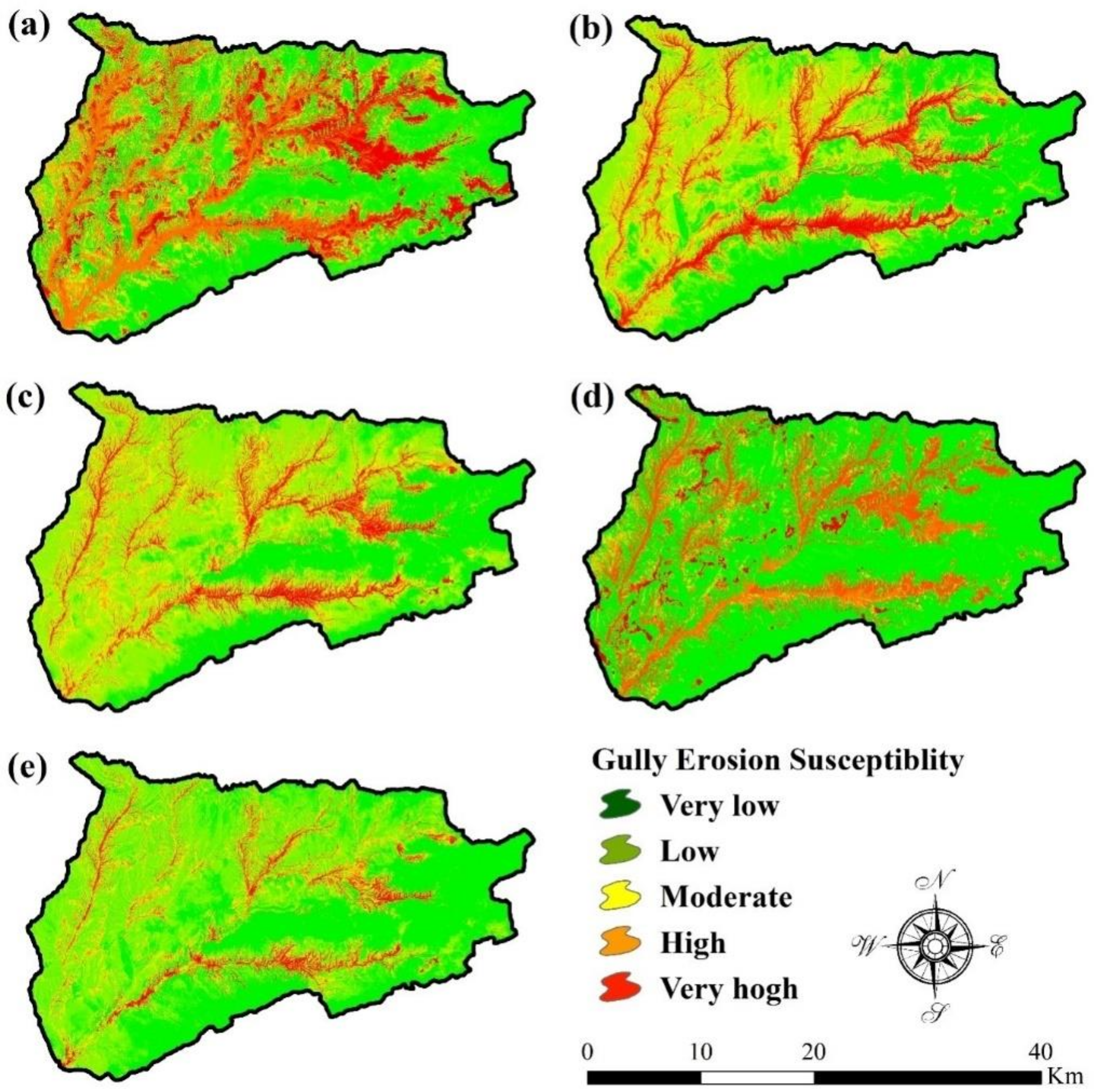
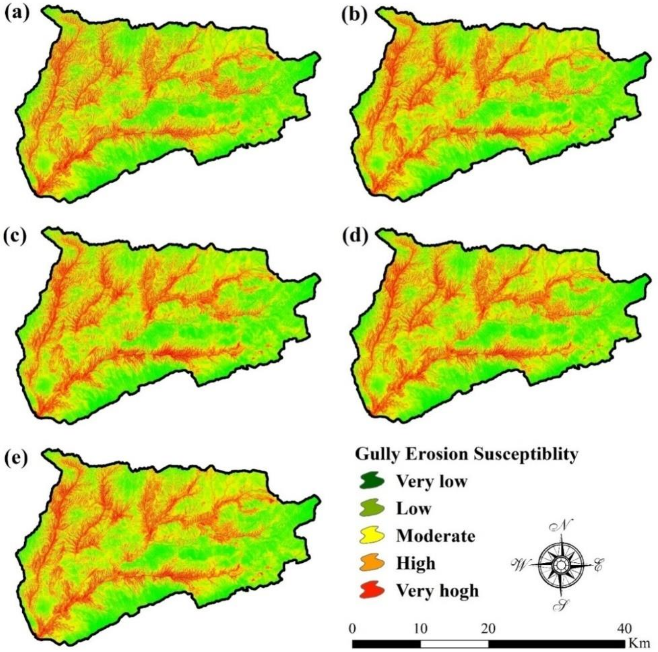
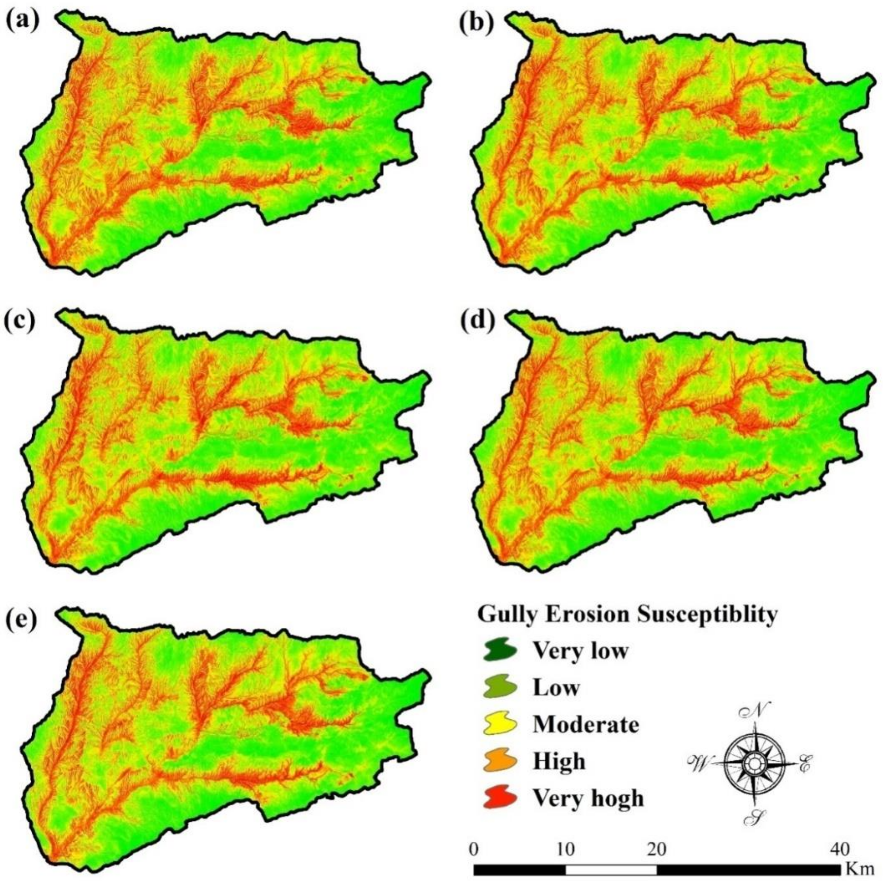
Gully erosion susceptibility was estimated by considering the ANN, GLM, MaxEnt, and SVM machine learning algorithms for this region. The overall data were randomly divided into different ratios (90/10, 80/20, 70/30, 60/40, and 50/50) as training and validation data to estimate the outcome of all predicted models with optimum accuracy. The all output raster of the susceptibility map was reclassified into different qualitative classes (very high, high, moderate, low, and very low) considering Jenks’ natural break classifier technique in the GIS environment.

3.2.1. Gully Erosion Susceptibility Modelling Using Artificial Neural Network (ANN)

The GESMs were prepared by using the ANN method in different sample ratios as training and validation data. In ANN, the overall data was randomly classified as training and validation data in different ratios (90/10, 80/20, 70/30, 60/40, and 50/50). The areal percentage in the ANN (90/10 ratio) model for very low, low, moderate, high, and very high gully erosion susceptible areas are 40.52%, 35.27%, 11.01%, 6.5%, and 6.7%, respectively (Figure 5a and Figure 6a). In the case of the ANN (80/20 ratio) model, the areal coverage for very low, low, moderate, high, and very high gully erosion susceptible areas are 64.47%, 3.90%, 4.30%, 8.13%, and 19.24%, respectively (Figure 5b). In the ANN (70/30 ratio) model, the areal percentage of very low, low, moderate, high, and very high gulling susceptible areas are 27.87%, 37.02%, 15.05%, 9.48%, and 10.57%, respectively (Figure 5c). The areal coverage percentage in the ANN (60/40 ratio) model for very low, low, moderate, high, and very high gully erosion susceptible areas are 39.09%, 23.94%, 13.75%, 10.23%, and 12.99%, respectively (Figure 5d). The areal coverage in the ANN (50/50 ratio) model for very low, low, moderate, high, and very high gully erosion susceptible areas are 44.07%, 9.05%, 8.52%, 19.14%, and 19.21%, respectively (Figure 5e).

3.2.2. Gully Erosion Susceptibility Modelling Using the General Linear Model (GLM)

The GESMs was prepared by using the GLM method in different sample sizes (random partitioning of the samples) as training and validation data. In GLM, the overall data was randomly classified as training and validation data in different ratios (90/10, 80/20, 70/30, 60/40, and 50/50). The areal percentage in the GLM (90/10 ratio) model for very low, low, moderate, high, and very high gully erosion susceptible areas are 23.93%, 23.10%, 21.19%, 17.78%, and 13.92%, respectively (Figure 6b and Figure 7a). The areal percentage in the GLM (80/20 ratio) model for very low, low, moderate, high, and very high gully erosion susceptible areas are 25.19%, 22.76%, 20.46%, 16.81%, and 14.77%, respectively (Figure 6b). The areal percentage in the GLM (70/30 ratio) model for very low, low, moderate, high, and very high gully erosion susceptible areas are 24.44%, 23.18%, 20.74%, 16.79%, and 14.86%, respectively (Figure 6c). The areal percentage in the GLM (60/40 ratio) model for very low, low, moderate, high, and very high gully erosion susceptible areas are 24.73%, 22.83%, 20.37%, 17.47%, and 14.59%, respectively (Figure 6d). The areal percentage in the GLM (50/50 ratio) model for very low, low, moderate, high, and very high gully erosion susceptible areas are 25.44%, 23.39%, 20.57%, 16.15%, and 14.47%, respectively (Figure 6e).

3.2.3. Gully Erosion Susceptibility Modelling Using Maximum Entropy (MaxEnt)

The GESMs were prepared by using the MaxEnt method in different sample sizes as training and validation data. In MaxEnt, the overall data was randomly classified as training and validation data in different ratios (90/10, 80/20, 70/30, 60/40, and 50/50). The areal percentage in the MaxEnt (90/10 ratio) model for very low, low, moderate, high, and very high gully erosion susceptible areas are 21.81%, 23.30%, 22.50%, 19.65%, and 13.75%, respectively (Figure 6c and Figure 8a). The areal percentage in the MaxEnt model (80/20 ratio) is 23.94%, 23.10 %, 21.05%, 17.61%, and 14.30%, respectively, for very low, moderate, high, and very high gully erosion susceptible areas (Figure 7b). The areal percentage in the MaxEnt (70/30 ratio) model for very low, low, moderate, high, and very high gully erosion susceptible areas are 22.32%, 21.80%, 22.14%, 19.81%, and 13.93%, respectively (Figure 7c). The areal percentage in the MaxEnt (60/40 ratio) model for very low, low, moderate, high, and very high gully erosion susceptible areas are 22.51%, 21.29%, 22.02%, 20.29%, and 13.90%, respectively (Figure 7d). The areal percentage in the MaxEnt (50/50 ratio) model for very low, low, moderate, high, and very high gully erosion susceptible areas are 23.39%, 22.14%, 22.63%, 17.95%, and 13.89%, respectively (Figure 7e).

3.2.4. Gully Erosion Susceptibility Modelling Using Support Vector Machine (SVM)

The GESMs were prepared by using the SVM method in different sample sizes as training and validation information. In SVM, the overall data was randomly classified as training and validation data in different ratios (90/10, 80/20, 70/30, 60/40, and 50/50). The areal percentages in the SVM (90/10 ratio) model for very low, low, moderate, high, and very high gully erosion susceptible areas are 29.89%, 20.78%, 18.32%, 15.99%, and 15.02%, respectively (Figure 8a). The areal percentages in the SVM (80/20 ratio) model for very low, low, moderate, high, and very high gully erosion susceptible areas are 30.66%, 20.98%, 17.56%, 15.94%, and 14.86%, respectively (Figure 8b and Figure 9d). The areal percentages in the SVM (70/30 ratio) model for very low, low, moderate, high, and very high gully erosion susceptible areas are 29.15%, 20.81%, 18.41%, 16.55%, and 15.08%, respectively (Figure 8c). The areal percentages in the SVM (60/40 ratio) model for very low, low, moderate, high, and very high gully erosion susceptible areas are 28.29%, 21.24%, 18.45%, 16.64%, and 15.38%, respectively (Figure 8d). The areal percentages in the SVM (50/50 ratio) model for very low, low, moderate, high, and very high gully erosion susceptible areas are 28.81%, 21.45%, 18.23%, 16.03%, and 15.48%, respectively (Figure 8e).

3.3. Assessing the Importance of the Factors

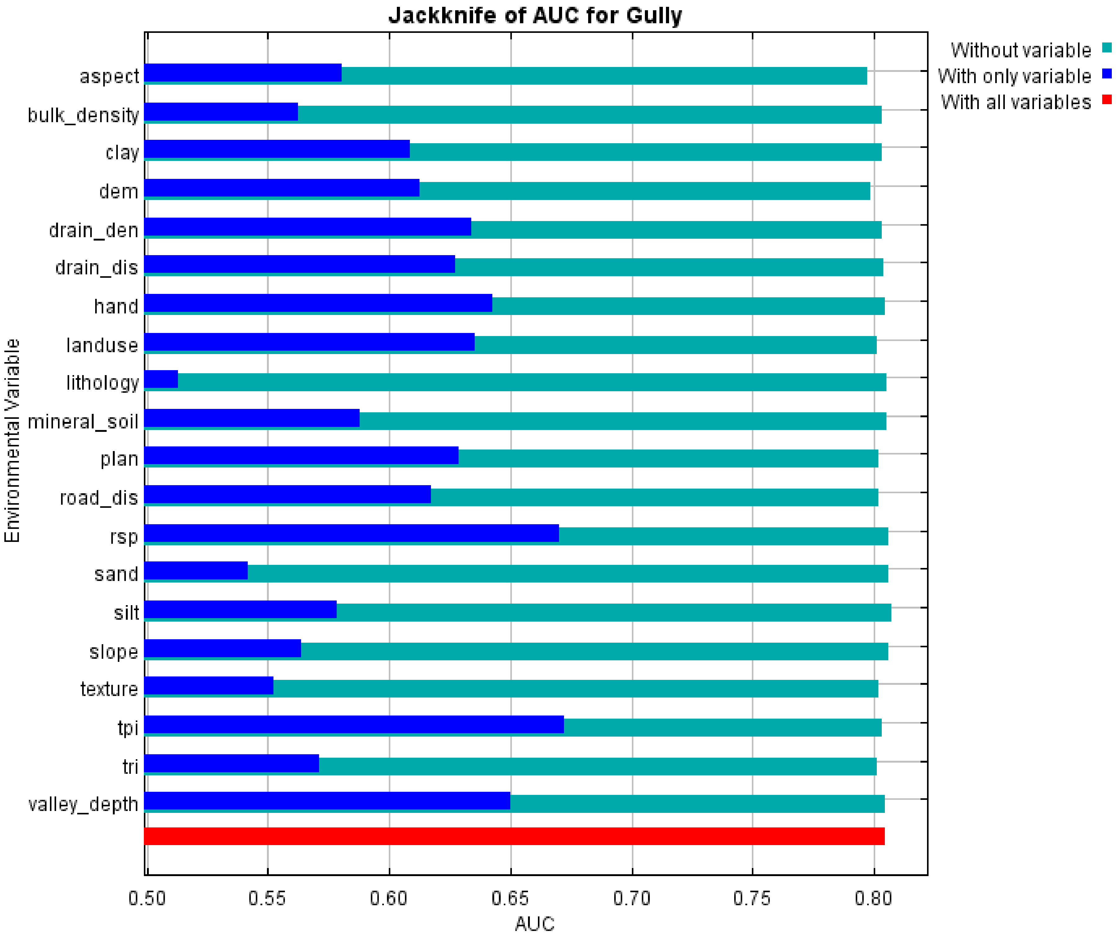
The importance of the variables for estimating the GESMs was estimated with the help of the jackknife AUC values. The maximum importance variables for gully erosion susceptibility are the topography position index (TPI), relative slope position (RSP), valley depth, height above nearest drainage (HAND), land use, drainage density, distance from river, plan curvature, and distance from road respectively. The lowest importance variables for gully erosion susceptibility are lithology, sand content, soil texture, slope, and elevation (Figure 10). The maximum and minimum importance variables for gully erosion susceptibility are the topography position index and lithology, with AUC values of 0.67 and 0.52, respectively. This type of assessment is helpful to estimate the importance of the variables and the influences of it in a dynamic way.

3.4. Validation of the Models

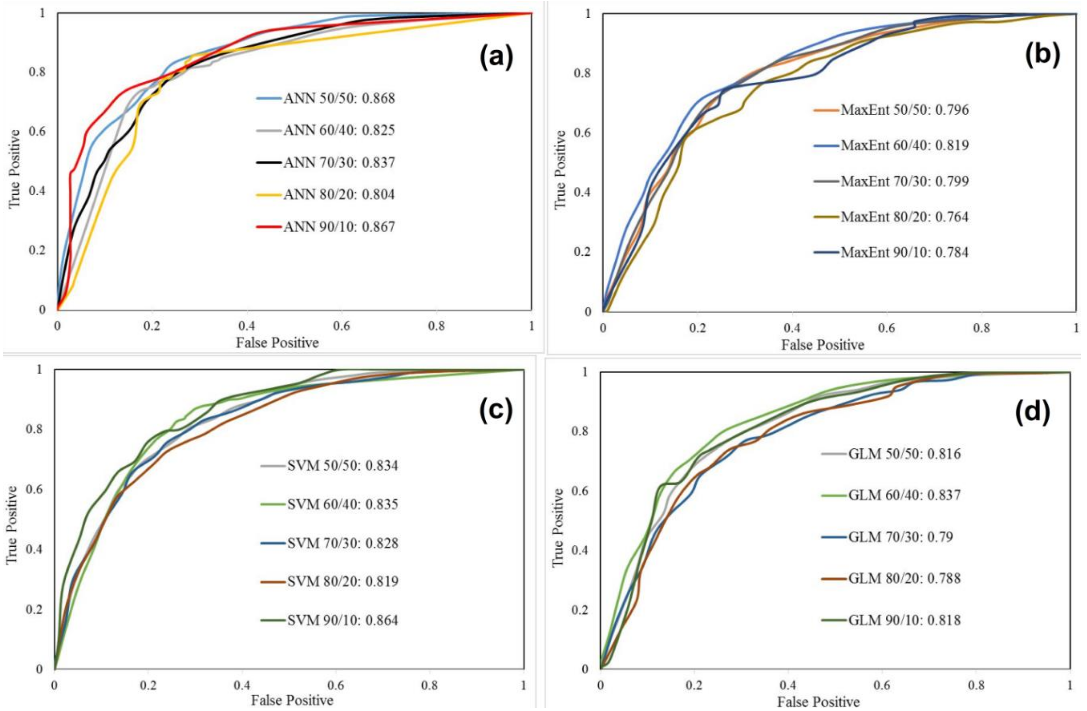
The accuracy of all predicted models was measured with the help of the area under curve (AUC) of the receiver operating characteristics (ROC) curve. It is a reliable tool for the accurate estimation of model performance. In the ANN model, the AUC values for the training datasets of 90/10, 80/20, 70/30, 60/40, and 50/50 are 0.885, 0.910, 0.872, 0.917, and 0.918, respectively (Figure 11). In the ANN model, the AUC values for the validation datasets of 90/10, 80/20, 70/30, 60/40, and 50/50 random partition are 0.867, 0.804, 0.837, 0.825, and 0.868, respectively (Figure 12).
In the case of the GLM model, the AUC values for the training datasets of 90/10, 80/20, 70/30, 60/40, and 50/50 random partitioning are 0.826, 0.834, 0.837, 0.813, and 0.833, respectively. In the GLM model, the AUC values for the validation datasets of 90/10, 80/20, 70/30, 60/40, and 50/50 random partition are 0.818, 0.788, 0.790, 0.837, and 0.816, respectively.
In the case of the MaxEnt model, the AUC values for the training datasets of 90/10, 80/20, 70/30, 60/40, and 50/50 random partitioning are 0.809, 0.821, 0.810, 0.786, and 0.808, respectively. In the MaxEnt model, the AUC values for the validation datasets of 90/10, 80/20, 70/30, 60/40, and 50/50 random partition are 0.784, 0.764, 0.799, 0.819, and 0.796, respectively.
In the case of the SVM model, the AUC values for the training datasets of 90/10, 80/20, 70/30, 60/40, and 50/50 random partitioning are 0.870, 0.877, 0.875, 0.859, and 0.866, respectively. In the SVM model, the AUC values for the validation datasets of 90/10, 80/20, 70/30, 60/40, and 50/50 random partition are 0.864, 0.819, 0.828, 0.835, and 0.834, respectively.

4. Discussion

Gully erosion is one of the common environmental issues caused by the natural environment, but the mechanism for the formation and development of gullies can accelerate by anthropogenic activities [23,52]. In the arid and semi-arid environment, the formation and development of gullies is the most problematic issue with global concerns that are related with ecological imbalances of the particular environment. The loss of fertile soil due to severe erosion not only reduces the amount of soil but also reduces soil fertility and associated agricultural productivity [42]. The climatic characteristics of this region relate to the semi-arid, semi-humid, and Mediterranean nature. The impact of extreme climatic conditions is therefore significant and has an impact on the large-scale erosion in the form of gullies. The formation and development of gullies is caused by different environmental conditions and their importance should be analyzed for appropriate modelling and management purposes [117].
The unpredictability of each outcome is mainly due to mechanisms beyond the researcher’s influence. Predictive accuracy is mostly based on the instability of both the quality of the data and the selection of the model [118]. Multiple factors can also be attributed to the unpredictability of gully erosion vulnerability models: (i) Insufficient experience of the physical environment and its associated mechanism, which must be analyzed; (ii) the distance over which the analysis can indeed be performed in each of these time or space; (iii) the randomization of the estimation method for the development of a model where gullies exist or are lacking; and (iv) an approximation for some computational method for the physical phenomenon [119]. In this work, our main objective was to highlight the susceptible areas with lees or marginal uncertainty within the predicted models.
In today’s research, the application of different machine learning algorithms is one of the reliable predicting tools for predicting the susceptibility of various natural hazards and disasters. For this purpose, different machine learning algorithms have been developed by different decision science researchers. In this regard, the spatial perspective of decision-making was considered to be the most reliable component in the various disciplines. Various machine learning models (e.g., ANN, GLM, MaxEnt, and SVM) are used in this study to estimate areas susceptible to gully erosion. In order to estimate results for better accuracy, the training and validation data were randomly divided into different quantities (e.g., 90/10, 80/20, 70/30, 60/40, and 50/50). ANN 50/50 is the best training and validation dataset model, although all models are associated with higher accuracy. According to the training datasets, apart from the ANN 50/50, other optimal models are ANN 60/40 (0.917), ANN 80/20 (0.910), and ANN 90/10 (0.885). According to the validation datasets, the most optimal model is ANN 50/50 (0.868) and other optimal models are ANN 90/10 (0.867), SVM 90/10 (0.864), and ANN 70/30 (0.837). The importance of all conditioning factors was estimated with the help of the jackknife test from the MaxEnt model. Jackknife checks the individual gully erosion conditional factor’s significance in the creation of the predicted models relative to all conditioning factors (red bars) for each predictor variable alone (blue bars), and the decrease in the training benefit when the variable is excluded from the overall model (navy green bars). The topography position index (TPI), relative slope position (RSP), valley depth, and height above nearest drainage (HAND) were recorded consistently as the key determinants of gully erosion, as also was the case in similar research [50,120,121,122]. The AUC values in the jackknife test of TPI, RSP, valley depth, and HAND are 0.67, 0.665, 0.65, and 0.64, respectively. Apart from this, the lower importance is associated with geological components like lithology (0.52) in gully erosion susceptibility modelling. The variable importance of other condition factors, i.e., aspect, bulk density, clay content, elevation, drainage density, distance from stream, land use, mineral soil, plan curvature, distance from road, sand, silt, slope, soil texture, and TRI, are 0.58, 0.56, 0.615, 0.62, 0.635, 0.63, 0.635, 0.585, 0.625, 0.62, 0.54, 0.575, 0.565, 0.552, and 0.575, respectively. From an evaluative point of view, the topographic indices themselves are not attributes that could be integrated with erosion at the same time. Strategic planners are therefore unable to start estimating soil erosion susceptibility on the basis of topographic indices. As a result, not only is the spatial dimension of erosion shown in the form of gullies, but it is also capable of giving us a theoretical framework and its associated cause–effect relationship between variables and associated erosion. Apart from this, the topographic variables may influence other factors of the condition that may have an influential role in the process of erosion. In this analysis, the maximum values of the TPI are most favorable for the development of large- and medium-sized gullies in the Golestan Dam Watershed as a whole. The relative slope position is one of the dominant factors in the control of pedogeomorphic processes and associated erosion. Higher valley depth is an important factor that directly accelerates the rate of large-scale erosion. In the wet season, the higher depth of the valley is recommended to severe erosion in the form of gullies, where rainfall and its associated runoff can play an essential role in this respect. Rainfall with high kinetic energy is associated with extensive erosion in most of the arid and semi-arid environments. It is also responsible for chemical weathering, which has an indirect effect on the rate of formation and development of the gully. This process confirms the transformation of the various minerals into secondary minerals. In this region, the process of water-induced erosion is accelerating to a height above the nearest drainage point. It is capable of controlling and determining river activity and associated erosion where primary direction and orientation play a vital role in the erosion process. The presence of vegetation in this region is very marginal in nature, and only a small part of the area is associated with agricultural activity, indicating the presence of bare soil and mountain topography with higher slopes. This association is most favorable to large-scale erosion in various forms of erosion, e.g., the creation and development of rills and gullies, etc. The absence of vegetation cover helps to create the maximum amount of runoff, which is directly and indirectly linked with erosion and its associated sedimentation. Higher amounts of rainfall and runoff indicated the greeter probability of erosion in any region. The maximum amount of the drainage network and the existence of gullies are positively linked with each other. The effects of rainfall and drainage during the wet season are not only favorable to the development of new gullies but are also responsible for the expansion of existing gullies. The formation of ephemeral gullies during the wet season is one of the main causes of serious erosion and loss of topsoil. The creation of ephemeral gullies and the associated loss of soil is a major problem in any arid and semi-arid environment. Furthermore, the impact of the road network is the result of the anthropogenic destruction of natural hydrological processes, establishing impervious soil surfaces accumulates runoff and results in large-scale soil erosion [41].
The erosion-prone gulling areas of this region were successfully assessed with an appropriate algorithm and random partitioning of the samples in order to maintain optimum accuracy. Prediction model accuracy was disturbed by a non-linear relationship, which is complex in nature [123,124]. Due to its role in the representation and disclosure of hidden properties and interactions, ANNs, implemented in an appropriate manner, can provide a robust replacement [112,125,126]. In contrast to any conventional simulation, ANN also has no limitations on the source and residual proportions [127,128]. The fault and lack of information can be resolved by ANN, and the presence of this type of inadequacy is capable of predicting the scenario with higher accuracy [129].

Models Prioritization

The final task was to select the optimal models according to their performance and related accuracy level. For this purpose, the prioritization of all predicted models for both training and validation databases was carried out with regard to the performance and robustness of accuracy. The prioritization method is generally used as a sub-catchment priority in morphometric studies with the consideration of different elements [130]. The same method was considered for the selection of the optimal model and the categorization of the models by performance. Based on training datasets that consider AUC values, the most optimal model is ANN 50/50 (0.918) followed by ANN 60/40 (0.917), ANN 80/20 (0885), ANN 90/10 (0.885), SVM 80/20 (0.877), SVM 70/30 (0.872), SVM 90/10 (0.87), SVM 50/50 (0.866), SVM 60/40 (0.859), GLM 70/30 (0.837), GLM 80/20 (0.834), GLM 50/50 (0.833), GLM 90/10 (0.826), MaxEnt 80/20 (0.821), GLM 60/40 (0.813), MaxEnt 70/30 (0.810), MaxEnt 90/10 (0.809), MaxEnt 50/50 (0.808), and MaxEnt 60/40 (0.786). Based on the validation datasets considering AUC values, the most optimal model is ANN 50/50 (0.868) followed by ANN 90/10 (0.867), SVM 90/10 (0.864), GLM 60/40 (0.837), ANN 70/30 (0.837), SVM 60/40 (0.835), SVM 50/50 (0.834), SVM 70/30 (0.828), ANN 60/40 (0.825), MaxEnt 60/40 (0.819), SVM 80/20 (0.819), GLM 90/10 (0.818), GLM 50/50 (0.816), ANN 80/20 (0.804), MaxEnt 70/30 (0.799), MaxEnt 50/50 (0.796), GLM 70/30 (0.79), GLM 80/20 (0.788), MaxEnt 90/10 (0.784), and MaxEnt 80/20 (0.764) (Table 5).

5. Conclusions

This region is severely confronted with the extreme problem of land degradation in different forms of erosion like the formation of rills, gullies etc. That is why not only the economy of this region is affected but the natural environment and its associated ecosystem are also affected a number of times. Apart from large-scale erosion, construction, such as roads, rail, and bridges, is also associated with large-scale erosion. Various machine learning approaches with random sample partitioning have been made to estimate the most accurate vulnerable regions with maximum possible accuracy. The main objective of this research was to determine the optimal model of gully erosion susceptibility in this region and the development of conceptual backgrounds for the orientation and partitioning of the data for prediction with maximum accuracy. Apart from this, with the random partitioning of the training and validation datasets, we are able to know the data handling model nature and its associated optimal capacity. In this research, the ANN (50/50) is the most optimal model for both training and validation data sets. The second and third optimal model considering the validation datasets were ANN 90/10, and SVM 90/10, respectively. Though, the ANN model in different random partitioning was not capable of estimation with maximum accuracy. This approach should be applicable in any part of the world with different climatic conditions. The role of the gully erosion conditioning factors is very much optimistic for the creation and development of gullies. In this region, the importance of the topographic parameters is the maximum for susceptibility to gully erosion compared to other parameters. Apart from secondary sources, an extensive field visit was carried out to validate the entire models’ outcome in a more precise way. The nature of the erosion and its impact on society was also identified at the time of the field visit. The impact of erosion in agricultural resources and the role of the stakeholders are the most conflicting issues in terms of sustainable land management practices. According to the ANN 50/50 model, 3.6.87% of the area of this watershed is associated with very high to moderate gully erosion susceptible zones. Most of the erosion-prone areas of this region are located near the drainage network. So, special watershed management strategies have to be incorporated in the vulnerable regions to escape this type of situation. It may be helpful to develop a conceptual background based on a theoretical perspective on the erosion of the gully, which may be applicable in different regions. Obviously, this type of outcome should be useful and applicable to decision-makers and local stakeholders in order to avoid this kind of serious problem by considering appropriate measures. The contribution and task of future research is to develop a model with the appropriate modification of the algorithm and partitioning of the samples and to link it to the socio-political environmental dilemma.

Author Contributions

Conceptualization, A.A.; Methodology, A.A.; formal analysis, A.A.; O.A.N.; investigation, A.A.; resources, A.A.; supervision, A.A.; writing—original draft preparation, A.A., S.C.P., R.C., A.S.; writing—review and editing, A.A., S.C.P., R.C., A.S., S.L., O.A.N., B.P., D.T.B. All authors have read and agreed to the published version of the manuscript.

Funding

This research received no external funding.

Acknowledgments

This research was supported by the Basic Research Project of the Korea Institute of Geoscience and M ineral Resources (KIGAM) and Project of Environmental Business Big Data Platform and Center Construction funded by the Ministry of Science and ICT.

Conflicts of Interest

The authors declare no conflict of interest.

References

  1. Magliulo, P. Assessing the susceptibility to water-induced soil erosion using a geomorphological, bivariate statistics-based approach. Environ. Earth Sci. 2012, 67, 1801–1820. [Google Scholar] [CrossRef]
  2. Arabameri, A.; Pradhan, B.; Rezaei, K.; Yamani, M.; Pourghasemi, H.R.; Lombardo, L. Spatial modelling of gully erosion using evidential belief function, logistic regression, and a new ensemble of evidential belief function–logistic regression algorithm. Land Degrad. Dev. 2018, 29, 4035–4049. [Google Scholar] [CrossRef]
  3. Pal, S.C.; Chakrabortty, R. Simulating the impact of climate change on soil erosion in sub-tropical monsoon dominated watershed based on RUSLE, SCS runoff and MIROC5 climatic model. Adv. Space Res. 2019, 64, 352–377. [Google Scholar] [CrossRef]
  4. Pal, S.C.; Chakrabortty, R. Modeling of water induced surface soil erosion and the potential risk zone prediction in a sub-tropical watershed of Eastern India. Modeling Earth Syst. Environ. 2019, 5, 369–393. [Google Scholar] [CrossRef]
  5. Pal, S.C.; Shit, M. Application of RUSLE model for soil loss estimation of Jaipanda watershed, West Bengal. Spat. Inf. Res. 2017, 25, 399–409. [Google Scholar] [CrossRef]
  6. Lal, R. Societal value of soil carbon. J. Soil Water Conserv. 2014, 69, 186A–192A. [Google Scholar] [CrossRef] [Green Version]
  7. Renard, K.; Yoder, D.; Lightle, D.; Dabney, S. 8 Universal Soil Loss Equation and Revised Universal Soil Loss Equation. In Handbook of Erososion Modelling; Morgan, R.P.C., Nearing, M., Eds.; Wiley: Hoboken, NJ, USA, 2011; Volume 137. [Google Scholar]
  8. Bobe, B.W. Evaluation of Soil Erosion in the Harerge Region of Ethiopia Using Soil Loss Models, Rainfall Simulation and Field Trials. Ph.D. Thesis, University of Pretoria, Pretoria, South Africa, 2005. [Google Scholar]
  9. Karimzadeh, H.; Alizadeh, M. Spatial estimation of soil erosion in Iran using RUSLE model. Iran. J. Ecohydrol. 2018. [Google Scholar] [CrossRef]
  10. Arabameri, A.; Chen, W.; Loche, M.; Zhao, X.; Li, Y.; Lombardo, L.; Cerda, A.; Pradhan, B.; Bui, D.T. Comparison of machine learning models for gully erosion susceptibility mapping. Geosci. Front. 2019. [Google Scholar] [CrossRef]
  11. Arabameri, A.; Rezaei, K.; Pourghasemi, H.R.; Lee, S.; Yamani, M. GIS-based gully erosion susceptibility mapping: A comparison among three data-driven models and AHP knowledge-based technique. Environ. Earth Sci. 2018, 77, 628. [Google Scholar] [CrossRef]
  12. Arabameri, A.; Pradhan, B.; Rezaei, K.; Conoscenti, C. Gully erosion susceptibility mapping using GIS-based multi-criteria decision analysis techniques. Catena 2019, 180, 282–297. [Google Scholar] [CrossRef]
  13. Torri, D.; Poesen, J.; Borselli, L.; Bryan, R.; Rossi, M. Spatial variation of bed roughness in eroding rills and gullies. Catena 2012, 90, 76–86. [Google Scholar] [CrossRef]
  14. Zhang, X.; Fan, J.; Liu, Q.; Xiong, D. The contribution of gully erosion to total sediment production in a small watershed in Southwest China. Phys. Geogr. 2018, 39, 246–263. [Google Scholar] [CrossRef]
  15. Rahmati, O.; Tahmasebipour, N.; Haghizadeh, A.; Pourghasemi, H.R.; Feizizadeh, B. Evaluation of different machine learning models for predicting and mapping the susceptibility of gully erosion. Geomorphology 2017, 298, 118–137. [Google Scholar] [CrossRef]
  16. Nampak, H.; Pradhan, B.; Mojaddadi Rizeei, H.; Park, H. Assessment of land cover and land use change impact on soil loss in a tropical catchment by using multitemporal SPOT-5 satellite images and R evised U niversal Soil L oss E quation model. Land Degrad. Dev. 2018, 29, 3440–3455. [Google Scholar] [CrossRef]
  17. Saha, A.; Ghosh, M.; Pal, S.C. Understanding the Morphology and Development of a Rill-Gully: An Empirical Study of Khoai Badland, West Bengal, India. In Gully Erosion Studies from India and Surrounding Regions; Springer: Cham, Switzerland, 2020; pp. 147–161. [Google Scholar]
  18. Imeson, A.; Kwaad, F. Gully types and gully prediction. Geografisch Tijdschrift 1980, 14, 430–441. [Google Scholar]
  19. Poesen, J. Contribution of gully erosion to sediment production. In Erosion and Sediment Yield: Global and Regional Perspectives, Proceedings of the International Symposium, Exeter, UK, 15–19 July 1996; Walling, D.E., Webb, B., Eds.; IAHS: Wallingford, UK, 1996; p. 251. [Google Scholar]
  20. Arabameri, A.; Pradhan, B.; Rezaei, K. Spatial prediction of gully erosion using ALOS PALSAR data and ensemble bivariate and data mining models. Geosci. J. 2019, 23, 669–686. [Google Scholar] [CrossRef]
  21. Kong, B.; Yu, H. Estimation model of soil freeze-thaw erosion in Silingco watershed wetland of northern Tibet. Sci. World J. 2013, 2013, 636521. [Google Scholar] [CrossRef]
  22. Guerra, A.J.T.; Fullen, M.A.; Jorge, M.d.C.; Bezerra, J.F.R.; Shokr, M.S. Slope processes, mass movement and soil erosion: A review. Pedosphere 2017, 27, 27–41. [Google Scholar] [CrossRef]
  23. Arabameri, A.; Pradhan, B.; Pourghasemi, H.R.; Rezaei, K.; Kerle, N. Spatial Modelling of Gully Erosion Using GIS and R Programing: A Comparison among Three Data Mining Algorithms. Appl. Sci. 2018, 8, 1369. [Google Scholar] [CrossRef] [Green Version]
  24. Kirkby, M.; Bracken, L. Gully processes and gully dynamics. Earth Surf. Process. Landf. J. Br. Geomorphol. Res. Group 2009, 34, 1841–1851. [Google Scholar] [CrossRef]
  25. Daba, S.; Rieger, W.; Strauss, P. Assessment of gully erosion in eastern Ethiopia using photogrammetric techniques. Catena 2003, 50, 273–291. [Google Scholar] [CrossRef]
  26. Gomez Gutierrez, A.; Schnabel, S.; Felicísimo, Á.M. Modelling the occurrence of gullies in rangelands of southwest Spain. Earth Surf. Process. Landf. J. Br. Geomorphol. Res. Group 2009, 34, 1894–1902. [Google Scholar] [CrossRef]
  27. Garosi, Y.; Sheklabadi, M.; Conoscenti, C.; Pourghasemi, H.R.; Van Oost, K. Assessing the performance of GIS-based machine learning models with different accuracy measures for determining susceptibility to gully erosion. Sci. Total Environ. 2019, 664, 1117–1132. [Google Scholar] [CrossRef]
  28. Arabameri, A.; Yamani, M.; Pradhan, B.; Melesse, A.; Shirani, K.; Bui, D.T. Novel ensembles of COPRAS multi-criteria decision-making with logistic regression, boosted regression tree, and random forest for spatial prediction of gully erosion susceptibility. Sci. Total Environ. 2019, 688, 903–916. [Google Scholar] [CrossRef]
  29. Seber, G.A.; Lee, A.J. Linear Regression Analysis; John Wiley & Sons: Hoboken, NJ, USA, 2012; Volume 329, ISBN 1-118-27442-3. [Google Scholar]
  30. Arabameri, A.; Pourghasemi, H.R. Spatial modeling of gully erosion using linear and quadratic discriminant analyses in GIS and R. In Spatial Modeling in GIS and R for Earth and Environmental Sciences; Elsevier: Amsterdam, The Netherlands, 2019; pp. 299–321. [Google Scholar]
  31. Arabameri, A.; Pourghasemi, H.R.; Yamani, M. Applying different scenarios for landslide spatial modeling using computational intelligence methods. Environ. Earth Sci. 2017, 76, 832. [Google Scholar] [CrossRef]
  32. Arabameri, A.; Lee, S.; Tiefenbacher, J.P.; Ngo, P.T.T. Novel Ensemble of MCDM-Artificial Intelligence Techniques for Groundwater-Potential Mapping in Arid and Semi-Arid Regions (Iran). Remote Sens. 2020, 12, 490. [Google Scholar] [CrossRef] [Green Version]
  33. Kujawski, E. Multi-Criteria Decision Analysis: Limitations, Pitfalls, and Practical Difficulties. 2003; Lawrence Berkeley National Laboratory: Berkley, CA, USA, 2007.
  34. Reilly, T. Making Hard Decisions with Decision Tools; Duxbury Thomson Learning: Boston, MA, USA, 2001; ISBN 0-534-36597-3. [Google Scholar]
  35. Conforti, M.; Aucelli, P.P.C.; Robustelli, G.; Scarciglia, F. Geomorphology and GIS analysis for mapping gully erosion susceptibility in the Turbolo stream catchment (Northern Calabria, Italy). Nat. Hazards 2011, 56, 881–898. [Google Scholar] [CrossRef]
  36. Rahmati, O.; Tahmasebipour, N.; Haghizadeh, A.; Pourghasemi, H.R.; Feizizadeh, B. Evaluating the influence of geo-environmental factors on gully erosion in a semi-arid region of Iran: An integrated framework. Sci. Total Environ. 2017, 579, 913–927. [Google Scholar] [CrossRef]
  37. Hosseinalizadeh, M.; Kariminejad, N.; Rahmati, O.; Keesstra, S.; Alinejad, M.; Mohammadian Behbahani, A. How can statistical and artificial intelligence approaches predict piping erosion susceptibility? Sci. Total Environ. 2019, 646, 1554–1566. [Google Scholar] [CrossRef]
  38. Zabihi, M.; Mirchooli, F.; Motevalli, A.; Khaledi Darvishan, A.; Pourghasemi, H.R.; Zakeri, M.A.; Sadighi, F. Spatial modelling of gully erosion in Mazandaran Province, northern Iran. Catena 2018, 161, 1–13. [Google Scholar] [CrossRef]
  39. Azareh, A.; Rahmati, O.; Rafiei-Sardooi, E.; Sankey, J.B.; Lee, S.; Shahabi, H.; Ahmad, B.B. Modelling gully-erosion susceptibility in a semi-arid region, Iran: Investigation of applicability of certainty factor and maximum entropy models. Sci. Total Environ. 2019, 655, 684–696. [Google Scholar] [CrossRef] [PubMed]
  40. Rahmati, O.; Haghizadeh, A.; Pourghasemi, H.R.; Noormohamadi, F. Gully erosion susceptibility mapping: The role of GIS-based bivariate statistical models and their comparison. Nat. Hazards 2016, 82, 1231–1258. [Google Scholar] [CrossRef]
  41. Arabameri, A.; Chen, W.; Lombardo, L.; Blaschke, T.; Tien Bui, D. Hybrid Computational Intelligence Models for Improvement Gully Erosion Assessment. Remote Sens. 2020, 12, 140. [Google Scholar] [CrossRef] [Green Version]
  42. Roy, P.; Chakrabortty, R.; Chowdhuri, I.; Malik, S.; Das, B.; Pal, S.C. Development of Different Machine Learning Ensemble Classifier for Gully Erosion Susceptibility in Gandheswari Watershed of West Bengal, India. In Machine Learning for Intelligent Decision Science; Rout, J.K., Rout, M., Das, H., Eds.; Algorithms for Intelligent Systems; Springer: Singapore, 2020; pp. 1–26. ISBN 9789811536885. [Google Scholar]
  43. Pourghasemi, H.R.; Yousefi, S.; Kornejady, A.; Cerdà, A. Performance assessment of individual and ensemble data-mining techniques for gully erosion modeling. Sci. Total Environ. 2017, 609, 764–775. [Google Scholar] [CrossRef] [Green Version]
  44. Amiri, M.; Pourghasemi, H.R.; Ghanbarian, G.A.; Afzali, S.F. Assessment of the importance of gully erosion effective factors using Boruta algorithm and its spatial modeling and mapping using three machine learning algorithms. Geoderma 2019, 340, 55–69. [Google Scholar] [CrossRef]
  45. Geissen, V.; Kampichler, C.; López-de Llergo-Juárez, J.J.; Galindo-Acántara, A. Superficial and subterranean soil erosion in Tabasco, tropical Mexico: Development of a decision tree modeling approach. Geoderma 2007, 139, 277–287. [Google Scholar] [CrossRef]
  46. Angileri, S.E.; Conoscenti, C.; Hochschild, V.; Märker, M.; Rotigliano, E.; Agnesi, V. Water erosion susceptibility mapping by applying Stochastic Gradient Treeboost to the Imera Meridionale River Basin (Sicily, Italy). Geomorphology 2016, 262, 61–76. [Google Scholar] [CrossRef]
  47. Hosseinalizadeh, M.; Kariminejad, N.; Chen, W.; Pourghasemi, H.R.; Alinejad, M.; Mohammadian Behbahani, A.; Tiefenbacher, J.P. Gully headcut susceptibility modeling using functional trees, naïve Bayes tree, and random forest models. Geoderma 2019, 342, 1–11. [Google Scholar] [CrossRef]
  48. Hosseinalizadeh, M.; Kariminejad, N.; Chen, W.; Pourghasemi, H.R.; Alinejad, M.; Mohammadian Behbahani, A.; Tiefenbacher, J.P. Spatial modelling of gully headcuts using UAV data and four best-first decision classifier ensembles (BFTree, Bag-BFTree, RS-BFTree, and RF-BFTree). Geomorphology 2019, 329, 184–193. [Google Scholar] [CrossRef]
  49. Gayen, A.; Pourghasemi, H.R. Spatial Modeling of Gully Erosion. In Spatial Modeling in GIS and R for Earth and Environmental Sciences; Elsevier: Amsterdam, The Netherlands, 2019; pp. 653–669. ISBN 978-0-12-815226-3. [Google Scholar]
  50. Saha, S.; Roy, J.; Arabameri, A.; Blaschke, T.; Tien Bui, D. Machine Learning-Based Gully Erosion Susceptibility Mapping: A Case Study of Eastern India. Sensors 2020, 20, 1313. [Google Scholar] [CrossRef] [Green Version]
  51. Varshney, K.R.; Alemzadeh, H. On the safety of machine learning: Cyber-physical systems, decision sciences, and data products. Big Data 2017, 5, 246–255. [Google Scholar] [CrossRef] [PubMed]
  52. Arabameri, A.; Asadi Nalivan, O.; Saha, S.; Roy, J.; Pradhan, B.; Tiefenbacher, J.P.; Thi Ngo, P.T. Novel Ensemble Approaches of Machine Learning Techniques in Modeling the Gully Erosion Susceptibility. Remote Sens. 2020, 12, 1890. [Google Scholar] [CrossRef]
  53. Javidan, N.; Kavian, A.; Pourghasemi, H.R.; Conoscenti, C.; Jafarian, Z. Data Mining Technique (Maximum Entropy Model) for Mapping Gully Erosion Susceptibility in the Gorganrood Watershed, Iran. In Gully Erosion Studies from India and Surrounding Regions; Shit, P.K., Pourghasemi, H.R., Bhunia, G.S., Eds.; Advances in Science, Technology & Innovation; Springer International Publishing: Cham, Switzerland, 2020; pp. 427–448. ISBN 978-3-030-23242-9. [Google Scholar]
  54. Garosi, Y.; Sheklabadi, M.; Pourghasemi, H.R.; Besalatpour, A.A.; Conoscenti, C.; Van Oost, K. Comparison of differences in resolution and sources of controlling factors for gully erosion susceptibility mapping. Geoderma 2018, 330, 65–78. [Google Scholar] [CrossRef]
  55. Pourghasemi, H.R.; Rossi, M. Landslide susceptibility modeling in a landslide prone area in Mazandarn Province, north of Iran: A comparison between GLM, GAM, MARS, and M-AHP methods. Theor. Appl. Clim. 2017, 130, 609–633. [Google Scholar] [CrossRef]
  56. De Reu, J.; Bourgeois, J.; Bats, M.; Zwertvaegher, A.; Gelorini, V.; De Smedt, P.; Chu, W.; Antrop, M.; De Maeyer, P.; Finke, P.; et al. Application of the topographic position index to heterogeneous landscapes. Geomorphology 2013, 186, 39–49. [Google Scholar] [CrossRef]
  57. Heerdegen, R.G.; Beran, M.A. Quantifying source areas through land surface curvature and shape. J. Hydrol. 1982, 57, 359–373. [Google Scholar] [CrossRef]
  58. Zevenbergen, L.W.; Thorne, C.R. Quantitative analysis of land surface topography. Earth Surf. Process. Landf. 1987, 12, 47–56. [Google Scholar] [CrossRef]
  59. Nobre, A.D.; Cuartas, L.A.; Hodnett, M.; Rennó, C.D.; Rodrigues, G.; Silveira, A.; Waterloo, M.; Saleska, S. Height Above the Nearest Drainage—A hydrologically relevant new terrain model. J. Hydrol. 2011, 404, 13–29. [Google Scholar] [CrossRef] [Green Version]
  60. Horton, R.E. Erosional development of streams and their drainage basins; hydrophysical approach to quantitative morphology. Geol. Soc Am. Bull. 1945, 56, 275. [Google Scholar] [CrossRef] [Green Version]
  61. Trigila, A.; Iadanza, C.; Esposito, C.; Scarascia-Mugnozza, G. Comparison of Logistic Regression and Random Forests techniques for shallow landslide susceptibility assessment in Giampilieri (NE Sicily, Italy). Geomorphology 2015, 249, 119–136. [Google Scholar] [CrossRef]
  62. Du, G.; Zhang, Y.; Iqbal, J.; Yang, Z.; Yao, X. Landslide susceptibility mapping using an integrated model of information value method and logistic regression in the Bailongjiang watershed, Gansu Province, China. J. Mt. Sci. 2017, 14, 249–268. [Google Scholar] [CrossRef]
  63. Amidon, G.E.; Secreast, P.J.; Mudie, D. Particle, Powder, and Compact Characterization. In Developing Solid Oral Dosage Forms; Elsevier: Amsterdam, The Netherlands, 2009; pp. 163–186. ISBN 978-0-444-53242-8. [Google Scholar]
  64. Rahmati, O.; Moghaddam, D.D.; Moosavi, V.; Kalantari, Z.; Samadi, M.; Lee, S.; Tien Bui, D. An Automated Python Language-Based Tool for Creating Absence Samples in Groundwater Potential Mapping. Remote Sens. 2019, 11, 1375. [Google Scholar] [CrossRef] [Green Version]
  65. Gallant, J.C.; Austin, J.M. Derivation of terrain covariates for digital soil mapping in Australia. Soil Res. 2015, 53, 895. [Google Scholar] [CrossRef]
  66. Conoscenti, C.; Agnesi, V.; Angileri, S.; Cappadonia, C.; Rotigliano, E.; Märker, M. A GIS-based approach for gully erosion susceptibility modelling: A test in Sicily, Italy. Environ. Earth Sci. 2013, 70, 1179–1195. [Google Scholar] [CrossRef]
  67. Ahmad, R. Landslides Processes, Prediction, and Land Use: Water Resources Monograph 18—By Roy C. Sidle and Hirotaka Ochiai. Nat. Resour. Forum 2007, 31, 322–323. [Google Scholar] [CrossRef]
  68. Chakrabortty, R.; Pal, S.C.; Sahana, M.; Mondal, A.; Dou, J.; Pham, B.T.; Yunus, A.P. Soil erosion potential hotspot zone identification using machine learning and statistical approaches in eastern India. Nat. Hazards 2020. [Google Scholar] [CrossRef]
  69. Garousi-Nejad, I.; Tarboton, D.G.; Aboutalebi, M.; Torres-Rua, A.F. Terrain Analysis Enhancements to the Height Above Nearest Drainage Flood Inundation Mapping Method. Water Resour. Res. 2019, 55, 7983–8009. [Google Scholar] [CrossRef]
  70. Horton, R.E. Drainage-basin characteristics. Trans. AGU 1932, 13, 350. [Google Scholar] [CrossRef]
  71. Conoscenti, C.; Angileri, S.; Cappadonia, C.; Rotigliano, E.; Agnesi, V.; Märker, M. Gully erosion susceptibility assessment by means of GIS-based logistic regression: A case of Sicily (Italy). Geomorphology 2014, 204, 399–411. [Google Scholar] [CrossRef] [Green Version]
  72. Althuwaynee, O.F.; Pradhan, B.; Park, H.-J.; Lee, J.H. A novel ensemble bivariate statistical evidential belief function with knowledge-based analytical hierarchy process and multivariate statistical logistic regression for landslide susceptibility mapping. Catena 2014, 114, 21–36. [Google Scholar] [CrossRef]
  73. Davoudi Moghaddam, D.; Rahmati, O.; Haghizadeh, A.; Kalantari, Z. A Modeling Comparison of Groundwater Potential Mapping in a Mountain Bedrock Aquifer: QUEST, GARP, and RF Models. Water 2020, 12, 679. [Google Scholar] [CrossRef] [Green Version]
  74. Pourghasemi, H.R.; Kerle, N. Random forests and evidential belief function-based landslide susceptibility assessment in Western Mazandaran Province, Iran. Environ. Earth Sci. 2016, 75, 185. [Google Scholar] [CrossRef]
  75. El Maaoui, M.A.; Sfar Felfoul, M.; Boussema, M.R.; Snane, M.H. Sediment yield from irregularly shaped gullies located on the Fortuna lithologic formation in semi-arid area of Tunisia. Catena 2012, 93, 97–104. [Google Scholar] [CrossRef]
  76. Wang, G.; Chen, X.; Chen, W. Spatial Prediction of Landslide Susceptibility Based on GIS and Discriminant Functions. IJGI 2020, 9, 144. [Google Scholar] [CrossRef] [Green Version]
  77. Chen, W.; Sun, Z.; Han, J. Landslide Susceptibility Modeling Using Integrated Ensemble Weights of Evidence with Logistic Regression and Random Forest Models. Appl. Sci. 2019, 9, 171. [Google Scholar] [CrossRef] [Green Version]
  78. Haykin, S. Neural Networks: A Comprehensive Foundation, 2nd ed.; Prentice Hall: Englewood Cliffs, NJ, USA, 1999. [Google Scholar]
  79. Cherkassky, V.; Krasnopolsky, V.; Solomatine, D.P.; Valdes, J. Computational intelligence in earth sciences and environmental applications: Issues and challenges. Neural Netw. 2006, 19, 113–121. [Google Scholar] [CrossRef]
  80. Kosko, B. Neural Networks and Fuzzy Systems: A Dynamical Systems Approach to Machine Intelligence; Prentice Hall: New York, NY, USA, 1992. [Google Scholar]
  81. Mandal, S.; Mondal, S. Statistical Approaches for Landslide Susceptibility Assessment and Prediction; Springer: Cham, Switzerland, 2019; ISBN 978-3-319-93897-4. [Google Scholar]
  82. Falaschi, F.; Giacomelli, F.; Federici, P.R.; Puccinelli, A.; D’Amato Avanzi, G.; Pochini, A.; Ribolini, A. Logistic regression versus artificial neural networks: Landslide susceptibility evaluation in a sample area of the Serchio River valley, Italy. Nat. Hazards 2009, 50, 551–569. [Google Scholar] [CrossRef]
  83. Gong, P.; Pu, R.; Chen, J. Elevation and forest-cover data using neural networks. Photogramm. Eng. Remote Sens. 1996, 62, 1249–1260. [Google Scholar]
  84. Hagan, M.T.; Demuth, H.B.; Beale, M.H.; De Jesus, O. Neural Network Design, 2nd ed.; Amazon Fulfillment Poland Sp. z o.o: Wrocław, Poland, 1996; ISBN 978-0-9717321-1-7. [Google Scholar]
  85. Lucà, F.; Conforti, M.; Robustelli, G. Comparison of GIS-based gullying susceptibility mapping using bivariate and multivariate statistics: Northern Calabria, South Italy. Geomorphology 2011, 134, 297–308. [Google Scholar] [CrossRef]
  86. McCullagh, P.; Nelder, J. Generalized Linear Models, 2nd ed.; Standard Book on Generalized Linear Models; Chapman and Hall: London, UK, 1989. [Google Scholar]
  87. Nelder, J.A.; Wedderburn, R.W. Generalized linear models. J. R. Stat. Soc. Ser. A (General) 1972, 135, 370–384. [Google Scholar] [CrossRef]
  88. Vorpahl, P.; Elsenbeer, H.; Märker, M.; Schröder, B. How can statistical models help to determine driving factors of landslides? Ecol. Model. 2012, 239, 27–39. [Google Scholar] [CrossRef]
  89. Maunder, M.N.; Punt, A.E. Standardizing catch and effort data: A review of recent approaches. Fish. Res. 2004, 70, 141–159. [Google Scholar] [CrossRef]
  90. Naghibi, S.A.; Pourghasemi, H.R. A comparative assessment between three machine learning models and their performance comparison by bivariate and multivariate statistical methods in groundwater potential mapping. Water Resour. Manag. 2015, 29, 5217–5236. [Google Scholar] [CrossRef]
  91. Bernknopf, R.L.; Campbell, R.H.; Brookshire, D.S.; Shapiro, C.D. A Probabilistic Approach to Landslide Hazard Mapping in Cincinnati, Ohio, with Applications for Economic Evaluation. Environ. Eng. Geosci. 1988, xxv, 39–56. [Google Scholar] [CrossRef]
  92. Woodbury, A.; Render, F.; Ulrych, T. Practical probabilistic ground-water modeling. Ground Water 1995, 33, 532–539. [Google Scholar] [CrossRef]
  93. Phillips, S.J.; Anderson, R.P.; Schapire, R.E. Maximum entropy modeling of species geographic distributions. Ecol. Model. 2006, 190, 231–259. [Google Scholar] [CrossRef] [Green Version]
  94. Phillips, S.J.; Dudík, M. Modeling of species distributions with Maxent: New extensions and a comprehensive evaluation. Ecography 2008, 31, 161–175. [Google Scholar] [CrossRef]
  95. Reddy, S.; Dávalos, L.M. Geographical sampling bias and its implications for conservation priorities in Africa. J. Biogeogr. 2003, 30, 1719–1727. [Google Scholar] [CrossRef]
  96. Kornejady, A.; Ownegh, M.; Bahremand, A. Landslide susceptibility assessment using maximum entropy model with two different data sampling methods. Catena 2017, 152, 144–162. [Google Scholar] [CrossRef]
  97. Phillips, S.J.; Dudík, M.; Elith, J.; Graham, C.H.; Lehmann, A.; Leathwick, J.; Ferrier, S. Sample selection bias and presence-only distribution models: Implications for background and pseudo-absence data. Ecol. Appl. 2009, 19, 181–197. [Google Scholar] [CrossRef] [Green Version]
  98. Elith, J.; Phillips, S.J.; Hastie, T.; Dudík, M.; Chee, Y.E.; Yates, C.J. A statistical explanation of MaxEnt for ecologists. Divers. Distrib. 2011, 17, 43–57. [Google Scholar] [CrossRef]
  99. Vapnik, V.; Guyon, I.; Hastie, T. Support vector machines. Mach. Learn 1995, 20, 273–297. [Google Scholar]
  100. Cristianini, N.; Shawe-Taylor, J. An Introduction to Support Vector Machines and Other Kernel-Based Learning Methods; Cambridge University Press: Cambridge, UK, 2000; ISBN 0-521-78019-5. [Google Scholar]
  101. Joachims, T. Text Categorization with Support Vector Machines: Learning with Many Relevant Features; Springer: Cham, Switzerland, 1998; pp. 137–142. [Google Scholar]
  102. Pradhan, B. A comparative study on the predictive ability of the decision tree, support vector machine and neuro-fuzzy models in landslide susceptibility mapping using GIS. Comput. Geosci. 2013, 51, 350–365. [Google Scholar] [CrossRef]
  103. Lee, S.; Hong, S.-M.; Jung, H.-S. A support vector machine for landslide susceptibility mapping in Gangwon Province, Korea. Sustainability 2017, 9, 48. [Google Scholar] [CrossRef] [Green Version]
  104. Yao, X.; Tham, L.; Dai, F. Landslide susceptibility mapping based on support vector machine: A case study on natural slopes of Hong Kong, China. Geomorphology 2008, 101, 572–582. [Google Scholar] [CrossRef]
  105. Yilmaz, I. Comparison of landslide susceptibility mapping methodologies for Koyulhisar, Turkey: Conditional probability, logistic regression, artificial neural networks, and support vector machine. Environ. Earth Sci. 2010, 61, 821–836. [Google Scholar] [CrossRef]
  106. Xu, C.; Xu, X.; Dai, F.; Saraf, A.K. Comparison of different models for susceptibility mapping of earthquake triggered landslides related with the 2008 Wenchuan earthquake in China. Comput. Geosci. 2012, 46, 317–329. [Google Scholar] [CrossRef]
  107. Hastie, T.; Tibshirani, R.; Friedman, J. The Elements of Statistical Learning: Data Mining, Inference, and Prediction; Springer Science & Business Media: Cham, Switzerland, 2009; ISBN 0-387-84858-4. [Google Scholar]
  108. Efron, B. The Jackknife, the Bootstrap and Other Resampling Plans; Society for Industrial and Applied Mathematics: Philadelphia, PA, USA, 1982; ISBN 978-0-89871-179-0. [Google Scholar]
  109. Bandos, A.I.; Guo, B.; Gur, D. Jackknife variance of the partial area under the empirical receiver operating characteristic curve. Stat. Methods Med. Res. 2017, 26, 528–541. [Google Scholar] [CrossRef] [Green Version]
  110. Convertino, M.; Troccoli, A.; Catani, F. Detecting fingerprints of landslide drivers: A MaxEnt model: Fingerprints of landslide drivers. J. Geophys. Res. Earth Surf. 2013, 118, 1367–1386. [Google Scholar] [CrossRef] [Green Version]
  111. Park, N.-W. Using maximum entropy modeling for landslide susceptibility mapping with multiple geoenvironmental data sets. Environ. Earth Sci. 2015, 73, 937–949. [Google Scholar] [CrossRef]
  112. Arabameri, A.; Cerda, A.; Rodrigo-Comino, J.; Pradhan, B.; Sohrabi, M.; Blaschke, T.; Tien Bui, D. Proposing a Novel Predictive Technique for Gully Erosion Susceptibility Mapping in Arid and Semi-arid Regions (Iran). Remote Sens. 2019, 11, 2577. [Google Scholar] [CrossRef] [Green Version]
  113. Roy, J.; Saha, S.; Arabameri, A.; Blaschke, T.; Bui, D.T. A Novel Ensemble Approach for Landslide Susceptibility Mapping (LSM) in Darjeeling and Kalimpong Districts, West Bengal, India. Remote Sens. 2019, 11, 2866. [Google Scholar] [CrossRef] [Green Version]
  114. Frattini, P.; Crosta, G.; Carrara, A. Techniques for evaluating the performance of landslide susceptibility models. Eng. Geol. 2010, 111, 62–72. [Google Scholar] [CrossRef]
  115. Pham, B.T.; Prakash, I. Evaluation and comparison of LogitBoost Ensemble, Fisher’s Linear Discriminant Analysis, logistic regression and support vector machines methods for landslide susceptibility mapping. Geocarto Int. 2019, 34, 316–333. [Google Scholar] [CrossRef]
  116. Fressard, M.; Thiery, Y.; Maquaire, O. Which data for quantitative landslide susceptibility mapping at operational scale? Case study of the Pays d’Auge plateau hillslopes (Normandy, France). Nat. Hazards Earth Syst. Sci. 2014, 14, 569–588. [Google Scholar] [CrossRef] [Green Version]
  117. Pourghasemi, H.R.; Sadhasivam, N.; Kariminejad, N.; Collins, A.L. Gully erosion spatial modelling: Role of machine learning algorithms in selection of the best controlling factors and modelling process. Geosci. Front. 2020. [Google Scholar] [CrossRef]
  118. Arabameri, A.; Cerda, A.; Pradhan, B.; Tiefenbacher, J.P.; Lombardo, L.; Bui, D.T. A methodological comparison of head-cut based gully erosion susceptibility models: Combined use of statistical and artificial intelligence. Geomorphology 2020, 359, 107136. [Google Scholar] [CrossRef]
  119. Conway, S.J.; Decaulne, A.; Balme, M.R.; Murray, J.B.; Towner, M.C. A new approach to estimating hazard posed by debris flows in the Westfjords of Iceland. Geomorphology 2010, 114, 556–572. [Google Scholar] [CrossRef] [Green Version]
  120. Razavi-Termeh, S.V.; Sadeghi-Niaraki, A.; Choi, S.-M. Gully erosion susceptibility mapping using artificial intelligence and statistical models. Geomat. Nat. Hazards Risk 2020, 11, 821–845. [Google Scholar] [CrossRef]
  121. Arabameri, A.; Pradhan, B.; Lombardo, L. Comparative assessment using boosted regression trees, binary logistic regression, frequency ratio and numerical risk factor for gully erosion susceptibility modelling. Catena 2019, 183, 104223. [Google Scholar] [CrossRef]
  122. Avand, M.; Janizadeh, S.; Naghibi, S.A.; Pourghasemi, H.R.; Khosrobeigi Bozchaloei, S.; Blaschke, T. A Comparative Assessment of Random Forest and k-Nearest Neighbor Classifiers for Gully Erosion Susceptibility Mapping. Water 2019, 11, 2076. [Google Scholar] [CrossRef] [Green Version]
  123. Chauchard, F.; Cogdill, R.; Roussel, S.; Roger, J.M.; Bellon-Maurel, V. Application of LS-SVM to non-linear phenomena in NIR spectroscopy: Development of a robust and portable sensor for acidity prediction in grapes. Chemom. Intell. Lab. Syst. 2004, 71, 141–150. [Google Scholar] [CrossRef] [Green Version]
  124. Raj Kiran, N.; Ravi, V. Software reliability prediction by soft computing techniques. J. Syst. Softw. 2008, 81, 576–583. [Google Scholar] [CrossRef]
  125. Yuan, H.; Yang, G.; Li, C.; Wang, Y.; Liu, J.; Yu, H.; Feng, H.; Xu, B.; Zhao, X.; Yang, X. Retrieving Soybean Leaf Area Index from Unmanned Aerial Vehicle Hyperspectral Remote Sensing: Analysis of RF, ANN, and SVM Regression Models. Remote Sens. 2017, 9, 309. [Google Scholar] [CrossRef] [Green Version]
  126. Fogno Fotso, H.R.; Aloyem Kazé, C.V.; Kenmoe, G.D. Optimal Input Variables Disposition of Artificial Neural Networks Models for Enhancing Time Series Forecasting Accuracy. Appl. Artif. Intell. 2020, 1–24. [Google Scholar] [CrossRef]
  127. Enke, D.; Thawornwong, S. The use of data mining and neural networks for forecasting stock market returns. Expert Syst. Appl. 2005, 29, 927–940. [Google Scholar] [CrossRef]
  128. Jha, M.K.; Sahoo, S. Efficacy of neural network and genetic algorithm techniques in simulating spatio-temporal fluctuations of groundwater: Neural network and genetic algorithm for groundwater level simulation. Hydrol. Process. 2015, 29, 671–691. [Google Scholar] [CrossRef]
  129. van Lint, J.W.C.; Hoogendoorn, S.P.; van Zuylen, H.J. Accurate freeway travel time prediction with state-space neural networks under missing data. Transp. Res. Part. C Emerg. Technol. 2005, 13, 347–369. [Google Scholar] [CrossRef]
  130. Chakrabortty, R.; Pal, S.C.; Chowdhuri, I.; Malik, S.; Das, B. Assessing the Importance of Static and Dynamic Causative Factors on Erosion Potentiality Using SWAT, EBF with Uncertainty and Plausibility, Logistic Regression and Novel Ensemble Model in a Sub-tropical Environment. J. Indian Soc. Remote Sens. 2020, 48, 765–789. [Google Scholar] [CrossRef]
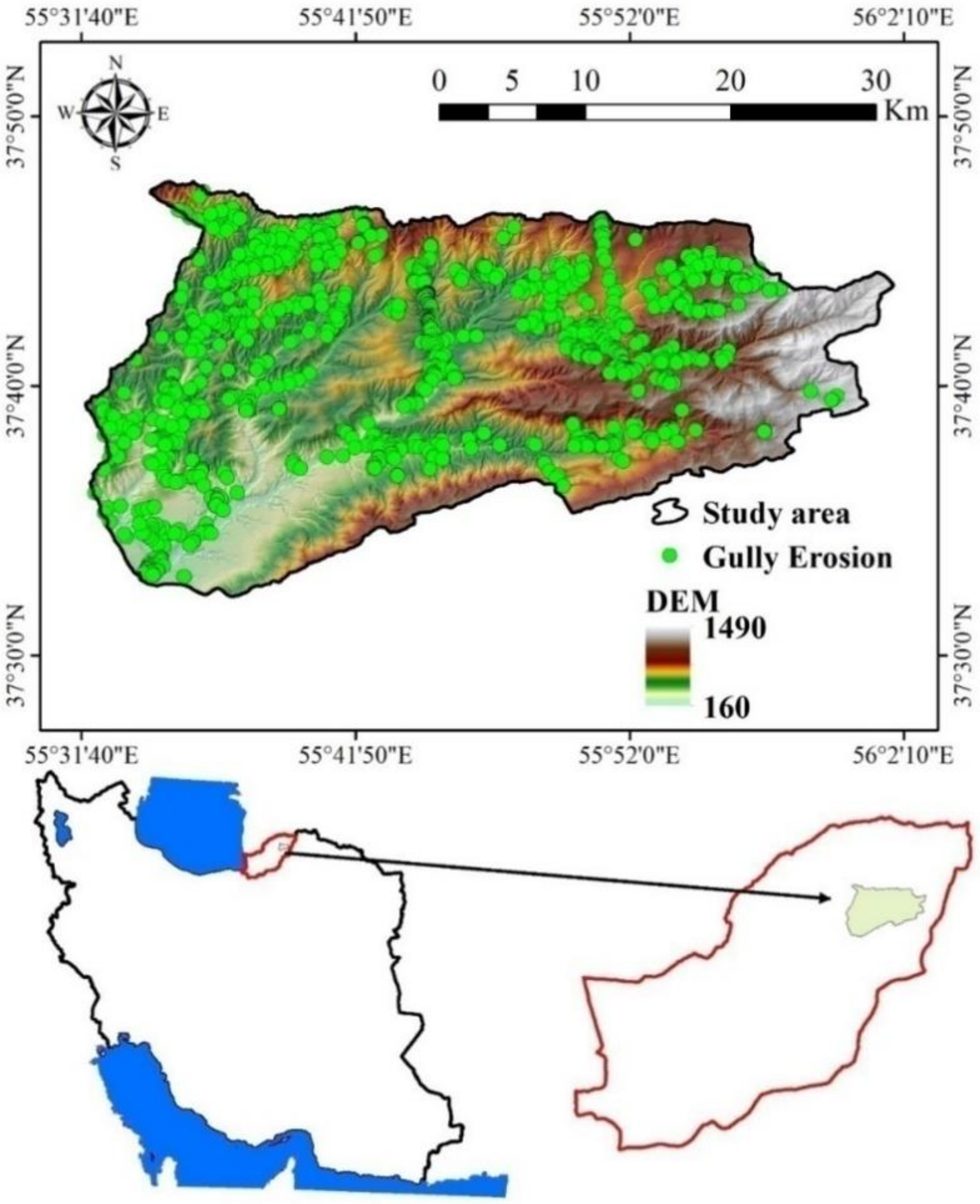
Figure 1. Location of the study area.
Remotesensing 12 02833 g001
Figure 2. Flowchart of research in the study area.
Remotesensing 12 02833 g002
Figure 3. Some of the mapped gullies in the study area. (a) Lat: 377012.3; Long 4183012. (b) Lat: 392812.6; Long 4176965.6. (c) Lat: 389226.2; Long 4173413.5.
Remotesensing 12 02833 g003
Figure 4. Gully erosion factors are showing (a) Topography position index (TPI), (b) Plan curvature, (c) Elevation, (d) Aspect, (e) Slope, (f) Height above nearest drainage (HAND), (g) Drainage density, (h) Distance from stream, (i) Terrain ruggedness index (TRI), (j) Distance from road, (k) Bulk density, (l) Mineral Soil, (m) Clay content, (n) Sand content, (o) Relative slope position (RSP), (p) Silt content, (q) Valley depth, (r) Land use, (s) Soil Texture, (t) Lithology.
Remotesensing 12 02833 g004aRemotesensing 12 02833 g004b
Figure 5. Gully erosion susceptibility mapping using the ANN model: (a) 50/50, (b) 60/40, (c) 70/30, (d) 80/20, and (e) 90/10.
Remotesensing 12 02833 g005
Figure 6. Gully erosion susceptibility mapping using the GLM model: (a) 50/50, (b) 60/40, (c) 70/30, (d) 80/20, (e) 90/10.
Remotesensing 12 02833 g006
Figure 7. Gully erosion susceptibility mapping using the MaxEnt model: (a) 50/50, (b) 60/40, (c) 70/30, (d) 80/20, (e) 90/10.
Remotesensing 12 02833 g007
Figure 8. Gully erosion susceptibility mapping using the SVM model: (a) 50/50, (b) 60/40, (c) 70/30, (d) 80/20, (e) 90/10.
Remotesensing 12 02833 g008
Figure 9. Area percent classes in the ANN (a), GLM (b), MaxEnt (c), and SVM (d) model.
Remotesensing 12 02833 g009
Figure 10. Jackknife test for important factors.
Remotesensing 12 02833 g010
Figure 11. Area under the curve based on training datasets in the ANN (a), MaxEnt (b), SVM (c), and GLM (d) model.
Remotesensing 12 02833 g011
Figure 12. Area under the curve based on validation datasets in the ANN (a), MaxEnt (b), SVM (c), and GLM (d) model.
Remotesensing 12 02833 g012
Table 1. Land use classes in the study area.
Land UseArea (he)Area (%)
Forest12,513.0415.95
Residential Areas498.60.64
Rangelands29,858.838.07
Agricultural35,568.245.35
Table 2. Lithology of the study area.
Geo UnitDescriptionAgeArea (ha)Area (%)
QmSwampCenozoic2169.482.77
QswGrey to block shale and thin layers of siltstone and sandstoneCenozoic58,000.9273.94
KsnAmmonite bearing shale with interaction of limestoneMesozoic9786.6312.48
KsrGrey thick—bedded limestone and dolomiteMesozoic4906.56.26
JmzOlive—green shale and sandstoneMesozoic1857.682.37
EkhSwampCenozoic1715.732.19
Table 3. Detailed information about the database.
Sl. No.Conditioning FactorsSourceTimeSpatial Resolution/Scale
1Topography position index (TPI)ALOSPALSER DEM12/08/201212.5 mt.
2Plan curvatureALOSPALSER DEM12/08/201212.5 mt.
3ElevationALOSPALSER DEM12/08/201212.5 mt.
4AspectALOSPALSER DEM12/08/201212.5 mt.
5SlopeALOSPALSER DEM12/08/201212.5 mt.
6Height above nearest drainage (HAND)ALOSPALSER DEM12/08/201212.5 mt.
7Drainage densityALOSPALSER DEM12/08/201212.5 mt.
8Distance from streamALOSPALSER DEM12/08/201212.5 mt.
9Train ruggness index (TRI)ALOSPALSER DEM12/08/201212.5 mt.
10Distance from roadGoogle Earth images, Landsat 8 satellite images by USGS and Topographical map by National Geographic Organization of Iran (www.ngo-org.ir)17/06/201930 mt.
11Bulk densitySoil and Water Research Institute (SWRI) (http://www.iran.swri.com)18/06/20191:1,000,000
12Mineral SoilSoil and Water Research Institute (SWRI) (http://www.iran.swri.com)18/06/20191:1,000,000
13Clay contentSoil and Water Research Institute (SWRI) (http://www.iran.swri.com)18/06/20191:1,000,000
14Sand contentSoil and Water Research Institute (SWRI) (http://www.iran.swri.com)18/06/20191:1,000,000
15Relative slope position (RSP)ALOSPALSER DEM12/08/201212.5 mt.
16Silt contentSoil and Water Research Institute (SWRI) (http://www.iran.swri.com)18/06/20191:1,000,000
17Valley depthALOSPALSER DEM12/08/201212.5 mt.
18Land useGoogle Earth images, Landsat 8 satellite images by USGS and Topographical map by National Geographic Organization of Iran (www.ngo-org.ir)17/06/201930 mt.
19Soil TextureSoil and Water Research Institute (SWRI) (http://www.iran.swri.com)18/06/20191:1,000,000
20LithologyGeological Society of Iran (GSI) (http://www.gsi.ir/)14/07/20191:100,000
Table 4. Multi-collinearity analysis of the gully conditioning factors.
Conditioning FactorsCollinearity Statistics
ToleranceVIF
TPI0.9231.079
HAND0.9211.118
Valley depth0.9161.124
Lithology0.9151.127
Land use0.8881.279
RSP0.8231.483
Bulk density0.8131.492
Distance from road0.7781.532
Soil texture0.7541.611
Plan0.7451.721
Distance from stream0.7431.865
Mineral Soil0.7391.897
Slope0.7281.932
Drainage density0.4252.364
TRI0.3872.624
Elevation0.3462.715
Aspect0.3452.817
Silt0.2333.534
Clay0.3133.696
Sand0.2314.749
Table 5. Area under the curve values of training and validation data in different divisions.
RowModelsAUCPrioritizing
TrainingValidationPriority Based on TrainingPriority Based on Validation
1GLM 90/100.8260.8181410
2GLM 80/200.8340.7881216
3GLM 70/300.8370.791115
4GLM 60/400.8130.837164
5GLM 50/500.8330.8161311
6MaxEnt 90/100.8090.7841817
7MaxEnt 80/200.8210.7641518
8MaxEnt 70/300.810.7991713
9MaxEnt 60/400.7860.819209
10MaxEnt 50/500.8080.7961914
11ANN 90/100.8850.86742
12ANN 80/200.910.804312
13ANN 70/300.8720.83774
14ANN 60/400.9170.82528
15ANN 50/500.9180.86811
16SVM 90/100.870.86483
17SVM 80/200.8770.81959
18SVM 70/300.8750.82867
19SVM 60/400.8590.835105
20SVM 50/500.8660.83496