Multi-View Polarimetric Scattering Cloud Tomography and Retrieval of Droplet Size

Abstract

Tomography aims to recover a three-dimensional (3D) density map of a medium or an object. In medical imaging, it is extensively used for diagnostics via X-ray computed tomography (CT). We define and derive a tomography of cloud droplet distributions via passive remote sensing. We use multi-view polarimetric images to fit a 3D polarized radiative transfer (RT) forward model. Our motivation is 3D volumetric probing of vertically-developed convectively-driven clouds that are ill-served by current methods in operational passive remote sensing. Current techniques are based on strictly 1D RT modeling and applied to a single cloudy pixel, where cloud geometry defaults to that of a plane-parallel slab. Incident unpolarized sunlight, once scattered by cloud-droplets, changes its polarization state according to droplet size. Therefore, polarimetric measurements in the rainbow and glory angular regions can be used to infer the droplet size distribution. This work defines and derives a framework for a full 3D tomography of cloud droplets for both their mass concentration in space and their distribution across a range of sizes. This 3D retrieval of key microphysical properties is made tractable by our novel approach that involves a restructuring and differentiation of an open-source polarized 3D RT code to accommodate a special two-step optimization technique. Physically-realistic synthetic clouds are used to demonstrate the methodology with rigorous uncertainty quantification.

1. Motivation, Context & Outline

Clouds play a significant role at local and global scales, affecting weather, the water cycle, solar power generation, and impacting the Earth’s energy balance [1]. Moreover, uncertainties in global climate models are significantly affected by our limited understanding, and therefore modeling, of cloud dynamics and microphysics [2]. Thus, understanding, modeling, and predicting cloud properties is a key issue with worldwide socio-economic implications that is in the center of many research studies [3]. Much of the current understanding relies on routine remote sensing of cloud properties such as by the MODerate resolution Imaging Spectrometer (MODIS) [4]. In practice, global-scale retrievals have so far been based on an individual pixel basis, using an approximation that clouds are plane-parallel slabs. This approximation uses a 1D radiative transfer (RT) model, which leads to biases in many retrievals [5] while other retrievals simply fail [6]. Convective clouds are therefore a blind spot due to their inherently 3D nature.

In its 2018 Decadal Strategy for Earth Observation from Space [7], the National Academies of Sciences, Engineering, and Medicine have indeed identified “Clouds, Convection, and Precipitation” as one of its five top-priority Targeted Variables for NASA’s next generation of satellite missions. To bridge this gap, new technology is needed to study clouds as 3D volumetric objects, on a global scale. The CloudCT [8] space mission, by the European Research Council (ERC), is specifically destined to provide data and products for this goal. It will involve 10 nano-satellites orbiting in formation, thus acquiring simultaneously unique multi-view measurements of such vertically-developed 3D clouds (Figure 1).

Moreover, common retrieval of cloud droplet characteristics use two optical bands simultaneously [9]: a visible band, where reflected radiance increases with cloud optical thickness, and a shortwave infra-red (SWIR) band, where absorption by condensed water depends on cloud droplet size. To sense droplet size in 3D by CloudCT or other future missions, sensors will need to have either SWIR or polarization capability.

1.1. Why Polarized Light?

There is an additional caveat in common retrievals, which rely on SWIR absorption [9]. In addition to absorption, light undergoes multiple scattering in clouds. Multiple scattering diminishes sensitivity to droplet microphysics. High sensitivity to microphysics is embedded in single-scattering events. It is thus beneficial to pick-up single-scatter signals, out of the strong multiply-scattered background radiance. Polarization signals of scattered light are dominated by single-scattering events, and are thus highly sensitive to the type and size specifications of scatters. Polarization therefore provides a significant signal for retrieval of droplet size distributions. In contrast, the intensity signal, which undergoes multiple-scattering events before reaching the sensor, is insensitive to the droplet size and provides complementary information about optical densities within the cloud.

In recent years, there is growing interest in polarimetric imagers for remote sensing of clouds and aerosols [10,11,12,13,14,15,16]. In turn, increased interest in polarimetric sensing capabilities has led to the development of 1D and 3D polarized (or “vector”) RT codes [17,18] with an aim of improving retrieval algorithms. Motivated by the CloudCT mission formulation—only the first of many to come in innovative passive cloud remote sensing—we develop herein a novel framework for 3D remote sensing of cloud properties using multi-view polarimetric measurements.

1.2. Why Passive Tomography?

From its etymology, the word “tomography” means a slice-by-slice recovery of an object’s 3D internal structure using 2D projections of cumulative density. In the computer age, this task is termed Computed Tomography (CT)  [19]. Common medical CT approaches are transmission-based X-ray CT or single-photon emission computed tomography (SPECT). There, 2D projections represent straight line-of-sight (LOS) integrals of the local X-ray opacity or nuclear marker density, respectively. In both imaging modalities, the inverse problem of recovering the medium content is linear [20].

Medical CT modalities generally use active radiation. Active methods are also used for atmospheric sensing or scatterers by radar and lidar. There, a transmitter and receiver are generally collocated and signals are based on backscattering and time-resolved two-way transmission. Probing is solved per LOS using methods which are computationally relatively simple. However, the technology is expensive, horizontal sampling is generally very limited, and irradiance decays fast from the transmitter. Passive sensing is less expensive, uses minimal power, and can image wide swaths of Earth. Thus global coverage mandates passive imaging from space. Consequently, this paper focuses on the derivation of 3D passive tomography of scatterer fields.

In passive imaging of scatterers, the light source irradiating the atmosphere is the sun: uncontrolled, steady and mono-directional. Passive remote sensing does not benefit from pulsed sources for echo-location. It should rely on multi-angular data. In general, however, retrieving atmospheric scatterer fields in 3D requires a full forward model of scattering in 3D. The model generalizes both the direct transmission model of linear CT and the diffusion limit. It can handle atmospheric regimes where neither a direct transmission model nor the diffusion limit are valid.

1.3. Context

In one sense or another, without tomography per se, three-dimensional cloud analysis using remote sensing data has been a topic of research for over two decades. There are well-known biases in optical thickness retrievals using the independent pixel approximation (IPA). To remove these biases, Marshak, et al. [21] invokes an inverse nonlocal IPA (NIPA). Marshak et al. [21] further demonstrates this approach on a single realization of a stochastic model for marine stratocumulus (Sc). NIPA is based on the RT Green’s function for horizontal (cross-pixel) transport of solar radiation between irradiation and escape to the above-head sensor, which can be computed numerically and conveniently parameterized. Using many instances of the same stochastic cloud model, neural networks (NNs) were successfully trained to retrieve domain-average cloud properties from nadir radiance fields [22,23,24]. Zinner et al. [25] generalized NIPA to multi-spectral retrievals of both optical thickness and column-averaged effective radius. Iwabuchi and Hayasaka [26] creatively combined NIPA-like physics-based and NN-like statistical regression methods to retrieve spatially varying properties of Sc clouds without suffering from IPA-induced biases.

Multi-angle Imaging Spectro-Radiometer (MISR)/Terra [27] was launched in 1999 and soon inspired research into cloud or cloud field reconstruction based on its unique multi-angle imaging capability. Marchand and Ackerman [28] used the original scalar version of the Spherical Harmonics Discrete Ordinates Method (SHDOM) iteratively to fit MISR observations of marine Sc by modifying the column optical thickness under each pixel. Other early pioneers were Seiz and Davies [29] who reconstructed the outer shell of a 2D transect through a large convective cloud by applying labor-intensive stereographic methods to MISR’s multi-angle imagery. Cornet and Davies [30] then estimated the mean optical thickness of that same cloud by performing repeated Monte Carlo 3D RT simulations, holding the outer shape constant, to fit the MISR radiometry. Evans et al. [31] trained a neural network to improve on the IPA retrieval of mean optical depth and its standard deviation using one or more MISR angles. To that effect, these last authors used SHDOM to compute multi-angle radiance fields from very many cloud fields generated with a Large Eddy Simulation (LES). This started a new trend in uncertainty quantification (UQ) in cloud remote sensing, using LES for ground truth that has by now become the standard, and used here as well.

There is a renewed interest in determining a cloud’s outer surface in its own right. On the one hand, very high resolution imagery from ground [32] or space [33] has been processed by stereophotogrammetric methods to generate dense “point clouds” representing many features seen from two cameras. On the other hand, the multi-view technique of “space carving”—used here for initializing the iterative tomography—defines the 3D region that contains a certain cloud by intersecting threshold-based cloud masks from multiple directions. Space carving methods have been applied to determine conservatively the outer shape of clouds observed with the airborne hyperangular Research Spectro-Polarimeter (RSP) [34], MISR [35] (same cloud as Reference [29]), and other sensors (e.g., References [36,37]). Note that methods based on cloud-masking, feature detection-and-tracking and/or stereoscopic location do not require radiometrically calibrated sensors. The loosened radiomeric use seems sub-optimal, since most sensors are in fact painstakingly calibrated to stringent (NIST-traceable) standards. Zinner et al. [38] have, to some extent, reconciled the notion of cloud surface sensing and RT-based cloud property estimation. Their approach scans the illuminated sides of vertically-developed convective clouds using a multispectral sensor mounted on an airborne platform. Then, a standard bi-spectral technique infers the vertical profile of cloud particle size along the side of the cloud. Alexandrov et al. [39] used LES clouds and 3D vector RT to demonstrate cloud-side microphysical profiling with RSP’s scanning polarimetric capability.

Remote sensing of clouds in complex 3D scenarios has already benefited from the advent of convolutional neural networks (CNNs), which excel in mapping one or more (e.g., multi-spectral) images, to inherent properties of the objects in the scene. The CNN is trained on a large database where the multi-spectral radiances are simulated with 3D RT and the pixel-scale cloud properties (typically, optical thickness and column-mean effective droplet radius) are known from the LES and assumed microphysics. Deep learning has thus been applied to both nadir satellite imagery [40] and to an array of ground-based sky cameras [41].

To close this non-exhaustive survey of cloud or cloud scene reconstruction techniques, we mention data fusion, which generally involves a combination of active and passive sensors. Liou et al. [42] blazed this path toward the inference of 3D cloud structure by creatively using a combination of ground-based mm-wave radar and multi-spectral imagery from a NOAA satellite overflying the same region. The radar delivers only a vertical 2D “curtain” of radar reflectivities from an extensive cirrus layer, while the multi-spectral imager provides raw information about the horizontal structure of the same cirrus layer. Barker et al. [43] used A-train satellite data (CloudSat, CALISPO, MODIS) to construct a plausible 3D cloud scene by populating off-nadir columns (where actively-probed profiles are lacking) by looking for a sub-satellite (hence actively profiled) pixel that is close in multi-spectral space. This “donor–receiver” algorithm is then iterated until a broadband 3D RT estimation of up-welling flux at the top of the atmosphere (TOA) agrees with the CERES measurement of it, thus satisfying a form of radiative closure. Fielding et al. [44] formalize cloud scene reconstruction with fused ground-based passive/active observations using an ensemble Kalman filter technique. Ensemble Kalman filtering is common in data assimilation for numerical weather prediction. Fielding et al. [44] assimilate observations into a suite of forward models based on 1D or 3D RT, however, rather than into the primitive equations of atmospheric dynamics.

1.4. Outline

Linear CT models (analogous to medical Xray CT and SPECT) were used to study gas emission and absorption in 3D plumes in the vicinity of pollution sources [45,46] or volcanoes [47,48]. There, Rayleigh-scattered sunlight was transmitted through the gas to a spectrometer on a platform flying around the plume. Following the vision of Werner et al. [49], Huang et al. [50,51] used scanning microwave radiometers to reconstruct 2D slices of particle density in clouds based on its impact on local emissivity. Linear CT was also adapted by Garay et al. [52] to characterize a smoke plume over water emanating from a coastal wild fire. There, the signal is sunlight scattered to space and detected by the Multi-angle Imaging Spectro-Radiometer (MISR) sensor [27] at nine viewing angles. The analysis in Reference [52] yields the direct transmission through the plume per LOS, from which linear CT analysis yields the plume density without using solar radiometers under the plume. Aides et al. [53] formulated CT based on single-scattered light. Their forward model is based on sets of broken-ray paths, where light changes direction once from the sun to a sensor. All the above atmospheric tomography methods assume the medium to be optically thin enough for direct and once-scattered radiation to dominate the measured radiance.

Biomedical imaging also involves CT modalities which are not based on linear models. A notable case in scattering-based tomography of X-ray CT is in Reference [54]. It exploits scattered radiation to obtain reconstruction with significantly lower dose and simpler acquisition hardware relative to linear CT systems, while enhancing estimation of chemical decomposition per volume element. Another example is Optical Diffusion Tomography (ODT) [55,56,57], which uses non-ionizing near-infrared light. It is worth noting the work by Che et al. [58] which departs from physics-based approaches into the realm of machine learning.

In contrast to ODT and the linear models described, which rely on either very high or very low orders of scattering, we use a steady-state polarized 3D RT forward model which generalizes far beyond these assumptions. This approach can seamlessly extract information about droplet sizes and densities from all orders of scattering.

Specifically, we adopt the vector Spherical Harmonics Discrete Ordinates Method (vSHDOM) [59,60], a popular computational 3D polarized RT model that, importantly here, is open source. We then formulate an inverse 3D RT problem for cloud tomography utilizing multi-view multi-spectral polarimetric images. In contrast to linear CT, the image formation model is nonlinear in the cloud’s microphysical and density variables. Our approach seeks an optimal fit of observed data to a physical model based on droplet microphysical and density parameters. Our work here generalizes our prior inversion approaches, which have been based on intensity-only observations [61,62,63,64,65]. Our generalization takes advantage of polarimetric measurements, thereby providing the benefits described in Section 1.1.

In Section 2, we cover basic cloud droplet optics using Mie scattering theory and the fundamentals of polarized 3D RT. The latter yields radiance which has a clear decomposition into single- and multiply-scattered light. This decomposition supports the solution to the inverse problem at hand. We then lay out our 3D cloud tomography method where we target three basic microphysical properties, volumetrically. Necessary but tedious mathematical details are presented in the Appendix A. Subsequently, the new 3D cloud tomographic capability is demonstrated on realistic synthetic clouds from an LES that provide ground truth for unambiguous retrieval error quantification. We conclude with a summary of our results and an outline of future developments, mostly looking toward CloudCT and other future space-based uses.

2. Theoretical Background

This section describes bulk microphysical parameterization of scattering media, the polarimetric radiative transfer image formation (forward) model and the relation between them. The section also describes the coordinate systems in use (per-scatterer, imager and Earth frames). We further decompose the polarized radiance into single-scattered and high-order scattered components. These foundations are used in subsequent sections, to formulate tomographic recovery. For concise reading, this section does not elaborate on some definitions. An extended, self-contained theoretical background section is given in Appendix A, which the readers are encouraged to follow to ease reproduction of our results.

2.1. Scatterer Microphysical Properties

In the lower atmosphere, cloud particles are droplets of liquid water that are very nearly spherical, having radius r. They are however polydisperse, with a droplet size distribution denoted $n\left(r\right)$. For most remote-sensing purposes, $n\left(r\right)$ is parameterized using an effective radius, $r_{\mathrm{e}}$ (in $\mu$m) and a dimensionless variance, $v_{\mathrm{e}}$ [66]. A commonly used parametric size distribution with empirical support [66] is the Gamma-distribution (Figure 2), detailed in Appendix A.1. Let ${\rho }_{\mathrm{w}}$ be the density of liquid water. An important cloud characteristic is the water mass density or Liquid Water Content (LWC) per unit volume. The parameters $r_{\mathrm{e}}$ and $v_{\mathrm{e}}$ dictate the shape of the droplet size distribution. LWC relates to droplet size and concentration, thus to optical opacity. In Section 3 the parameters $\mathrm{LWC},r_{\mathrm{e}},v_{\mathrm{e}}$ are unknown quantities, which we seek to estimate on a 3D grid.

2.2. Single Scattering of Polarized Light

In the absence of molecular absorption, material optical properties can be approximated using a single wavelength for each spectral band. This approximation, commonly used in multi-spectral remote sensing, relies on a single rendering of spectrally-averaged optical properties. It is valid if wavelength dependencies within a spectral band are weak, a condition met when narrow bands are considered. Macroscopic optical cross-sections are then expressed as averages weighted by the size-distribution $n\left(r\right)$. We respectively denote the extinction, scattering and absorption cross-sections as

$$\begin{array}{c}\hfill {\sigma }_{\mathrm{t}}\left(\lambda \right),{\sigma }_{\mathrm{s}}\left(\lambda \right),{\sigma }_{\mathrm{a}}\left(\lambda \right).\end{array}$$

(1)

Note that throughout the text, dependency on $\lambda$ is generally omitted for simplicity; however, it is used at specific points as needed.

Scattering, as a fraction of the overall interaction [67], is expressed by the dimensionless single scattering albedo

$$\begin{array}{c}\hfill \varpi =\frac{{\sigma }_{\mathrm{s}}}{{\sigma }_{\mathrm{t}}}.\end{array}$$

(2)

The extinction coefficient (or optical density), denoted by $\beta$, is expressed in terms of the LWC as [68]

$$\begin{array}{c}\hfill \beta =\mathrm{LWC}·{\tilde{\sigma }}_{\mathrm{t}}.\end{array}$$

(3)

Here, ${\tilde{\sigma }}_{\mathrm{t}}$ is the mass extinction coefficient (in units of ${\mathrm{m}}^2/\mathrm{g}$).

Let $\mathbf{\omega }$ and ${\mathbf{\omega }}^{\prime }$ be the unitary incident and scattered ray direction vectors respectively in Figure 2. Single-scattering geometry is defined by the local coordinate system of the incoming beam’s electric fields. The electric field of incoming light is decomposed into components along orthogonal directions. We set them as

$${\mathbf{E}}_1\propto \mathbf{\omega }\times {\mathbf{\omega }}^{\prime },{\mathbf{E}}_2\propto {\mathbf{E}}_1\times \mathbf{\omega }.$$

(4)

The scattering angle is $\theta ={cos}^{-1}(\mathbf{\omega }·{\mathbf{\omega }}^{\prime })$. The angular redistribution of singly-scatterred light by a volume element is defined by the macroscopic phase matrix $\mathbf{P}\left(\theta \right)$. For spherical (or just randomly-oriented) particles, the phase-matrix $\mathbf{P}\left(\theta \right)$ takes the following symmetric form [66]

$$\begin{array}{c}\hfill \mathbf{P}\left(\theta \right)=\left[\begin{array}{cccc}{p}_{11}\left(\theta \right)& p_{21}\left(\theta \right)& 0& 0\\ p_{21}\left(\theta \right)& p_{22}\left(\theta \right)& 0& 0\\ 0& 0& p_{33}\left(\theta \right)& -p_{43}\left(\theta \right)\\ 0& 0& p_{43}\left(\theta \right)& p_{44}\left(\theta \right)\end{array}\right],\end{array}$$

(5)

where $p_{11}$ is the (unpolarized) scattering phase-function.

It is convenient to define the state of polarized light in terms of the Stokes [66] vector $\mathbf{I}={\left(I,Q,U,V\right)}^{\top }$, where I is the unpolarized intensity. The Stokes components relate to statistics of the fields ${\mathbf{E}}_1,{\mathbf{E}}_2$ mentioned in Equation (4), as described in Appendix A.2. The degrees of polarization (DOP) and linear polarization (DoLP) are respectively defined as the ratios $\sqrt{Q^2+U^2+V^2}/I,\sqrt{Q^2+U^2}/I$. The angle of linear polarization (AoLP) is $1/2{tan}^{-1}(U/Q)$. Referring to the matrix elements in Equation (5), in single-scattering of unpolarized incident sunlight, the DoLP of scattered light amounts to the ratio $|p_{21}|/p_{11}$.

Mie Scattering

Mie theory describes how light interacts with a spherical particle of size comparable to $\lambda$ [69]. Denote $\mu =cos\theta$. Scattering of the Stokes vector $\mathbf{I}$ is described by the phase matrix ${\mathbf{P}}_{\mathrm{Mie}}\left(\mu \right)$, which is fully defined by six matrix components:

$$p_{11}^{\mathrm{Mie}}\left(\mu \right),p_{12}^{\mathrm{Mie}}\left(\mu \right),p_{22}^{\mathrm{Mie}}\left(\mu \right),p_{33}^{\mathrm{Mie}}\left(\mu \right),p_{43}^{\mathrm{Mie}}\left(\mu \right),p_{44}^{\mathrm{Mie}}\left(\mu \right).$$

(6)

Expressions of Mie and Rayleigh scattering phase matrices are given in Appendix A.3.

Mie scattering due to water droplets peaks at specific angles. For a single droplet or monodisperse material, ${\mathbf{P}}^{\mathrm{Mie}}$ has sharp scattering lobes at angles that depend on the droplet’s $r/\lambda$ ratio. A macroscopic voxel contains droplets in a range of radii r, smoothing the scattering lobes. The smoothing effect depends on $v_{\mathrm{e}}$ (Figure 3). Two angular domains that stand out for remote-sensing purposes are the cloud-bow ($\theta \in [{135}^{°},{155}^{°}]$) and glory ($\theta \in [{175}^{°},{180}^{°}]$). Both domains have peaks that are sensitive to the droplet microphysical parameters, and are significantly polarized (i.e., peaks are visible in the $p_{12}^{\mathrm{Mie}}$ component). The latter fact renders these peaks distinguishable in the presence of a multiply-scattered signal component.

2.3. Multiple Scattering of Polarized Light

The Radiative Transfer Equation (RTE) [70] describes multiple scattering interactions of monochromatic partially polarized light within a medium. Transmittance between two points $x_1,x_2$ is

$$\begin{array}{c}\hfill T\left(x_1\to x_2\right)=exp\left[-{\int }_{x_1}^{x_2}\beta \left(x\right)\mathrm{d}x\right].\end{array}$$

(7)

An atmospheric domain $\Omega$ is bounded by $\partial \Omega$. The intersection of $\partial \Omega$ with a ray originating at point $x$ in direction $-\mathbf{\omega }$ (Figure 4) is denoted $x_0(x,\omega )$. Denote the Stokes vector field as $\mathbf{I}\left(x,\mathbf{\omega }\right)$. Then $\mathbf{I}(x_0,\mathbf{\omega })$ is the Stokes vector of radiation which propagates in direction $\mathbf{\omega }$ at boundary point $x_0\left(x,\mathbf{\omega }\right)$. The non-emissive forward RT model [70] couples $\mathbf{I}\left(x,\mathbf{\omega }\right)$ to a vector source field $\mathbf{J}\left(x,\mathbf{\omega }\right)$ (Figure 4) by

$$\begin{array}{ccc}& & \mathbf{I}\left(x,\mathbf{\omega }\right)=\mathbf{I}(x_0,\mathbf{\omega })T\left(x_0\to x\right)+{\int }_{x_0}^x\mathbf{J}(x^{\prime },\mathbf{\omega })\beta \left(x^{\prime }\right)T\left(x^{\prime }\to x\right)\mathrm{d}{x}^{\prime },\hfill \end{array}$$

(8)

$$\begin{array}{ccc}& & \mathbf{J}\left(x,\mathbf{\omega }\right)=\frac{\varpi \left(x\right)}{4\pi }{\int }_{4\pi }\mathbf{P}\left(x,\mathbf{\omega }·{\mathbf{\omega }}^{\prime }\right)\mathbf{I}\left(x,{\mathbf{\omega }}^{\prime }\right)\mathrm{d}{\mathbf{\omega }}^{\prime }.\hfill \end{array}$$

(9)

Equations (8) and (9) are solved numerically, either directly with an explicit solver [60] or indirectly using a Monte-Carlo path tracer [71]. We use vSHDOM [60] to simulate scattered Stokes components of a realistic atmosphere, having both Mie and Rayleigh scattering due to water droplets and air molecules.

Multiple scattering interactions are defined using two coordinate systems. Local scatterer coordinates are set by $({\widehat{\mathbf{E}}}_1,{\widehat{\mathbf{E}}}_2)$. Stokes measurements in satellites, however, are defined in Meridional coordinates. Let $\widehat{\mathbf{z}}$ denote the zenith direction vector at every point on Earth. In meridian coordinates, the electric field components are defined by direction vectors

$$\begin{array}{c}\hfill {\widehat{\mathbf{m}}}_1=\frac{\widehat{\mathbf{z}}\times \mathbf{\omega }}{\parallel \widehat{\mathbf{z}}\times \mathbf{\omega }\parallel },{\widehat{\mathbf{m}}}_2=\mathbf{\omega }\times {\widehat{\mathbf{m}}}_1.\end{array}$$

(10)

Each pixel-scale Stokes measurement is described by a coordinate system defined by ${\widehat{\mathbf{m}}}_1$ and ${\widehat{\mathbf{m}}}_2$. The transformation between the two coordinate systems amounts to a multiplication of $\mathbf{I}$ by a Mueller rotation matrix.

Sampling $\mathbf{I}\left(x,\mathbf{\omega }\right)$ at the location of each camera and direction of each camera pixel yields the measured Stokes vector. A measurement k is taken at the camera position $x_k$, LOS direction ${\mathbf{\omega }}_k$, and wavelength ${\lambda }_k$ (Figure 4). Thus, Equations (8) and (9) yield the pixel measurement model

$$\begin{array}{c}\hfill \mathbf{I}\left[k\right]=\mathbf{I}\left(x_0,{\mathbf{\omega }}_k\right)T\left(x_0\to x_k\right)+{\int }_{x_0}^{x_k}\mathbf{J}\left(x^{\prime },{\mathbf{\omega }}_k\right)\beta \left(x^{\prime }\right)T\left(x^{\prime }\to x_k\right)\mathrm{d}{x}^{\prime }.\end{array}$$

(11)

2.4. Single-Scattering Separation

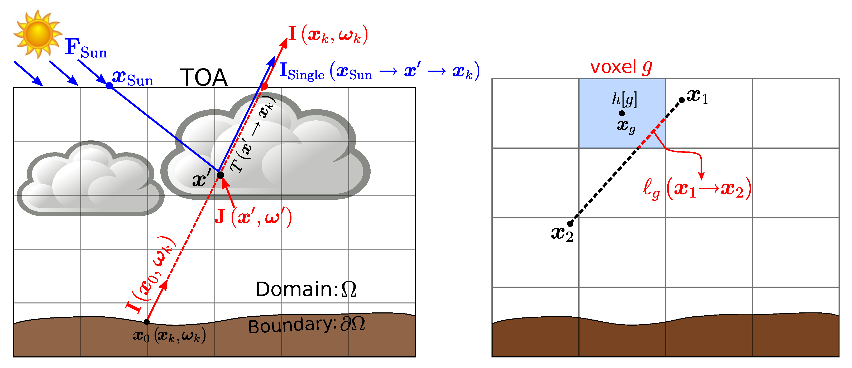
It is often convenient to separate the single-scattering contribution from the rest of the radiance field [72]. The solar irradiance at the top of the atmosphere (TOA) is $F_{\mathrm{Sun}}$. It is unoplarized, thus corresponds to a Stokes vector ${\mathbf{F}}_{\mathrm{Sun}}={\left(F_{\mathrm{Sun}},0,0,0\right)}^{\top }$. The Sun is modeled as an ideal directional source with direction ${\mathbf{\omega }}_{\mathrm{Sun}}$. A solar ray heading to point $x$ intersects the TOA at point $x_{\mathrm{Sun}}$. The solar transmittance is given by $T\left(x_{\mathrm{Sun}}\to x\right)$. Let $\delta$ denote Dirac’s delta. Thus, $\mathbf{I}$ can be written as a sum of the diffuse component ${\mathbf{I}}_{\mathrm{d}}$, and direct solar component:

$$\mathbf{I}\left(x,\mathbf{\omega }\right)={\mathbf{I}}_{\mathrm{d}}\left(x,\mathbf{\omega }\right)+\delta \left(\mathbf{\omega }-{\mathbf{\omega }}_{\mathrm{Sun}}\right){\mathbf{F}}_{\mathrm{Sun}}T\left(x_{\mathrm{Sun}}\to x\right).$$

(12)

Inserting (12) into (9) yields

$$\mathbf{J}\left(x,\mathbf{\omega }\right)={\mathbf{J}}_{\mathrm{d}}\left(x,\mathbf{\omega }\right)+\frac{\varpi \left(x\right)}{4\pi }\mathbf{P}\left(x,\mathbf{\omega }·{\mathbf{\omega }}_{\mathrm{Sun}}\right){\mathbf{F}}_{\mathrm{Sun}}T\left(x_{\mathrm{Sun}}\to x\right),$$

(13)

where

$${\mathbf{J}}_{\mathrm{d}}\left(x,\mathbf{\omega }\right)=\frac{\varpi \left(x\right)}{4\pi }{\int }_{4\pi }\mathbf{P}\left(x,\mathbf{\omega }·{\mathbf{\omega }}^{\prime }\right){\mathbf{I}}_{\mathrm{d}}\left(x,{\mathbf{\omega }}^{\prime }\right)\mathrm{d}{\mathbf{\omega }}^{\prime }.$$

(14)

Consider Figure 4. It shows a broken-ray path of direct sunlight, which undergoes single scattering at $x^{\prime }$, then reaches the camera at $x_k$. Denote this broken ray by

$$x_{\mathrm{Sun}}\to x^{\prime }\to x_k.$$

(15)

The direction vector between $x^{\prime }$ and $x_k$ is ${\mathbf{\omega }}_k$. This broken ray projects to a pixel corresponding to ${\mathbf{\omega }}_k$ at camera location $x_k$ thus contributing to the measurement $\mathbf{I}(x_k,{\mathbf{\omega }}_k)$. Using Equations (8) and (13), the single-scattered contribution from $x^{\prime }$ is

$$\begin{array}{c}\hfill {\mathbf{I}}_{\mathrm{Single}}\left(x_{\mathrm{Sun}}\to x^{\prime }\to x_k\right)=\frac{\varpi \left(x^{\prime }\right)}{4\pi }\beta \left(x^{\prime }\right)\mathbf{P}\left(x^{\prime },{\mathbf{\omega }}_k·{\mathbf{\omega }}_{\mathrm{Sun}}\right){\mathbf{F}}_{\mathrm{Sun}}T\left(x_{\mathrm{Sun}}\to x^{\prime }\right)T\left(x^{\prime }\to x_k\right).\end{array}$$

(16)

Thus, the entire single-scattered signal accumulates contributions along the LOS

$${\mathbf{I}}_{\mathrm{Single}}\left(x_k\right)={\int }_{x_0}^{x_k}{\mathbf{I}}_{\mathrm{Single}}\left(x_{\mathrm{Sun}}\to x^{\prime }\to x_k\right)\mathrm{d}{x}^{\prime }.$$

(17)

2.5. Ray Tracing

Ray tracing computes a function over a straight line through a 3D domain. A common operation is path-integration (e.g., Equations (7) and (8)). Let $h\left(x\right)$ be a continuous field. Define a grid of discrete points $x_g,\mathrm{where}g=1,2,\dots ,N_{\mathrm{grid}}$. Denote $h\left[g\right]=h\left(x_g\right)$. A path-integral over $h\left(x\right)$ is numerically computed using an interpolation kernel K

$$\begin{array}{c}\hfill {\int }_{x_1}^{x_2}h\left(x\right)\mathrm{d}x=\sum _{g=1}^{N_{\mathrm{grid}}}h\left[g\right]{\int }_{x_1}^{x_2}K\left(x-x_g\right)\mathrm{d}x.\end{array}$$

(18)

For zero-order interpolation (i.e., voxel grid), (18) degenerates to

$$\begin{array}{c}\hfill {\int }_{x_1}^{x_2}h\left(x\right)\mathrm{d}x=\sum _{g=1}^{N_{\mathrm{grid}}}h\left[g\right]{\ell }_g\left(x_1\to x_2\right),\end{array}$$

(19)

where ${\ell }_g\left(x_1\to x_2\right)$ is the intersection of the path with voxel g (Figure 4). For voxel indices g that do not intersect the path $x_1\to x_2$, the value of ${\ell }_g\left(x_1\to x_2\right)$ is 0.

3. Cloud Tomography

So far, we described the forward (image-formation) model, that is, how images are formed, given cloud properties. In this work, we formulate a novel inverse tomographic problem of recovering the unknown cloud microphysical properties, volumetrically. In voxel g, the vector of unknown parameters is $\left(\mathrm{LWC}\left[g\right],r_{\mathrm{e}}\left[g\right],v_{\mathrm{e}}\left[g\right]\right)$. The unknown microphysical parameters are concatenated to a vector of length $3N_{\mathrm{grid}}$

$$\Theta ={\left(\dots ,\mathrm{LWC}\left[g\right],r_{\mathrm{e}}\left[g\right],v_{\mathrm{e}}\left[g\right],\dots \right)}^{\top },1\le g\le N_{\mathrm{grid}}.$$

(20)

Neglecting circular polarization, each pixel measures a Stokes vector, ${\mathbf{y}}_{\mathbf{I}}=\left(y_{\mathrm{I}},y_{\mathrm{Q}},y_{\mathrm{U}}\right)$ at $N_{\lambda }$ wavelengths. Let $N_{\mathrm{views}}$ and $N_{\mathrm{pix}}$ denote the number of view points and camera pixels. The total number of Stokes measurements is thus $N_{\mathrm{meas}}=N_{\lambda }{N}_{\mathrm{views}}{N}_{\mathrm{pix}}$. The measurement vector of length $3N_{\mathrm{meas}}$ is expressed as

$$\mathbf{y}={\left({\mathbf{y}}_{\mathbf{I}}\left[1\right],\dots ,{\mathbf{y}}_{\mathbf{I}}\left[N_{\mathrm{meas}}\right]\right)}^{\top }.$$

(21)

In this section, we formulate the use of measurements $\mathbf{y}$ (multi-view, multi-pixel, multi-spectral, polarimetric measurements) for tomographic retrieval of $\Theta$ (3D volumetric cloud density and microphysics). It is worth mentioning at this point that the Stokes components are not measured directly. Rather, they are computationally retrieved from measurements taken using different states of polarization filters (see Appendix C for the AirMSPI measurement model).

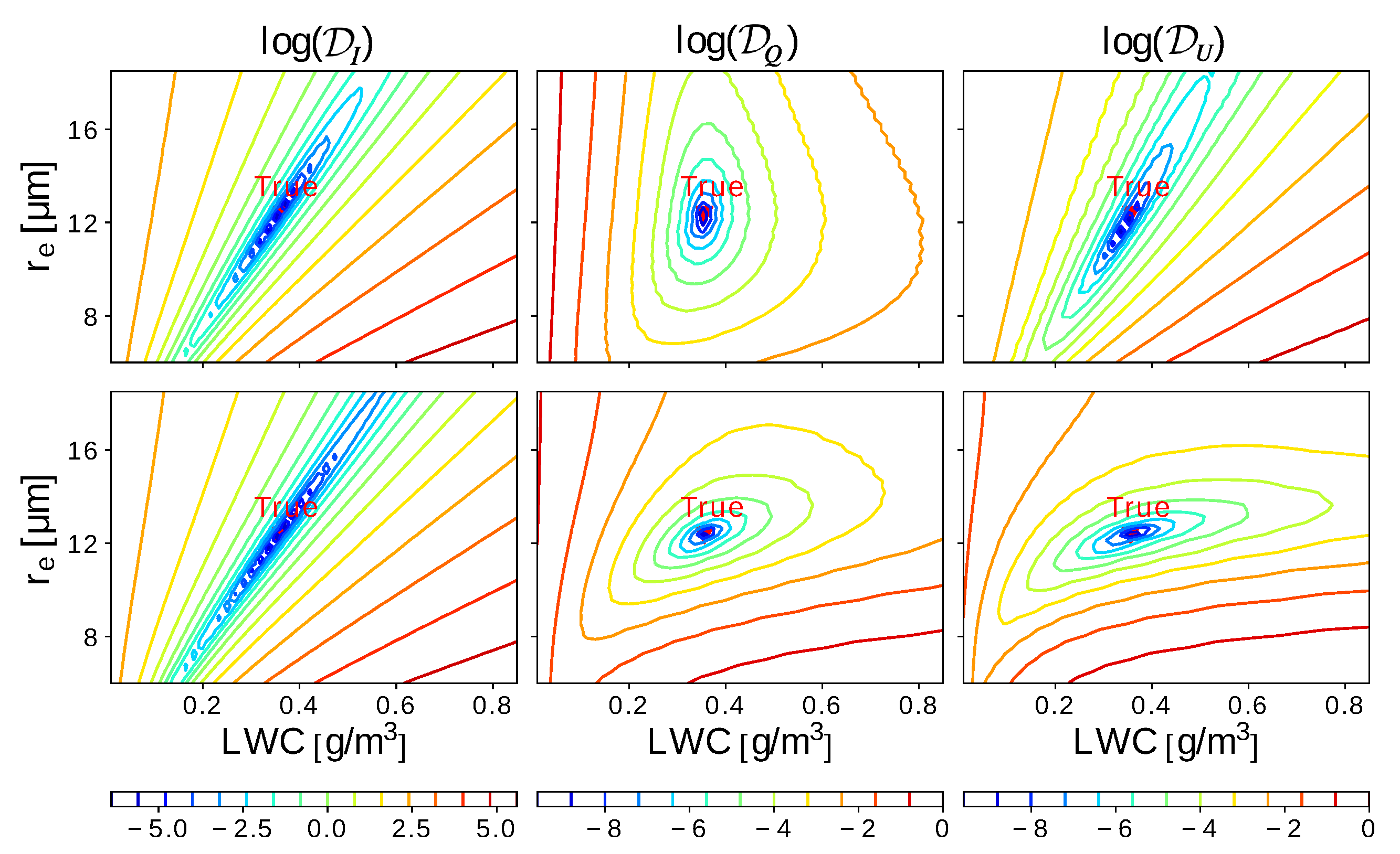
3.1. Polarimetric Information

To make an initial assessment of the sensitivity of polarimetric measurements, we simulate a simple homogeneous cubic cloud (Figure 5), parameterized by two microphysical parameters: $(\mathrm{LWC},r_{\mathrm{e}})$. Back-scattered Stokes measurements are taken at the TOA for the same angles and wavelengths as sampled by the Airborne Multi-angle Spectro-Polarimetric Imager (AirMSPI) [14]. AirMSPI is used here as a proxy instrument to demonstrate our approach. However, the approach is applicable to other polarimetric imagers.

Let $I\left[k\right],U\left[k\right],Q\left[k\right]$ be simulated Stokes components at measurement index k, and let $v_{\mathrm{e}}$ be held constant. Define a cost (data-misfit) function for each of the Stokes components

$$\begin{array}{ccc}\hfill {\mathcal{D}}_{\mathrm{I}}\left(\mathrm{LWC},r_{\mathrm{e}}\right)& =& \sum _{k=1}^{N_{\mathrm{meas}}}{\left(I\left[k\right]-y_{\mathrm{I}}\left[k\right]\right)}^2,\hfill \end{array}$$

(22)

$$\begin{array}{ccc}\hfill {\mathcal{D}}_{\mathrm{Q}}\left(\mathrm{LWC},r_{\mathrm{e}}\right)& =& \sum _{k=1}^{N_{\mathrm{meas}}}{\left(Q\left[k\right]-y_{\mathrm{Q}}\left[k\right]\right)}^2,\hfill \end{array}$$

(23)

$$\begin{array}{ccc}\hfill {\mathcal{D}}_{\mathrm{U}}\left(\mathrm{LWC},r_{\mathrm{e}}\right)& =& \sum _{k=1}^{N_{\mathrm{meas}}}{\left(U\left[k\right]-y_{\mathrm{U}}\left[k\right]\right)}^2.\hfill \end{array}$$

(24)

Equations (22)–(24) are 2D manifolds. Figure 6 plots the cost manifolds for different solar azimuth angles, ${\varphi }_0$. While there is an ambiguity between $\mathrm{LWC}$ and $r_{\mathrm{e}}$ when relying on ${\mathcal{D}}_{\mathrm{I}}$, there are better defined minima for ${\mathcal{D}}_{\mathrm{Q}}$ and ${\mathcal{D}}_{\mathrm{U}}$. This indicates that polarization measurements carry valuable information.

3.2. Inverse Problem Formulation

Denote ${\mathbf{I}}_{\Theta }$ as the image formation model. Tomography can be formulated as minimization of a data-fit function. We perform

$$\begin{array}{c}\hfill \widehat{\Theta }=\underset{\Theta }{argmin}\mathcal{D}\left({\mathbf{I}}_{\Theta },\mathbf{y}\right)=\underset{\Theta }{argmin}{\left({\mathbf{I}}_{\Theta }-\mathbf{y}\right)}^{\top }{\Sigma }^{-1}\left({\mathbf{I}}_{\Theta }-\mathbf{y}\right),\end{array}$$

(25)

Here $\Sigma$ is related to the co-variance matrix of the measurement noise. For brevity, we omit the subscript $\Theta$ but remember that

$$\mathbf{I}\equiv {\mathbf{I}}_{\Theta },\mathbf{J}\equiv {\mathbf{J}}_{\Theta },\beta \equiv {\beta }_{\Theta },\varpi \equiv {\varpi }_{\Theta },\mathbf{P}\equiv {\mathbf{P}}_{\Theta },T\equiv T_{\Theta }.$$

(26)

Assuming noise in different pixels, wavelengths and angles is uncorrelated, (25) degenerates to

$$\widehat{\Theta }=\underset{\Theta }{argmin}\sum _{k=1}^{N_{\mathrm{meas}}}{\left(\mathbf{I}\left[k\right]-{\mathbf{y}}_{\mathbf{I}}\left[k\right]\right)}^{\top }{\mathbf{R}}^{-1}\left(\mathbf{I}\left[k\right]-{\mathbf{y}}_{\mathbf{I}}\left[k\right]\right).$$

(27)

The matrix $\mathbf{R}$ depends on the particular sensor technology. Description of $\mathbf{R}$, tailored to the AirMSPI sensor, is detailed in Appendix C.

We solve (27) by a gradient-based approach. The gradient with respect to the unknown parameters $\Theta$ is

$$\begin{array}{c}\hfill {\nabla }_{\Theta }\mathcal{D}\left({\mathbf{I}}_{\Theta },\mathbf{y}\right)=2\sum _{k=1}^{N_{\mathrm{meas}}}{\left(\mathbf{I}\left[k\right]-{\mathbf{y}}_{\mathbf{I}}\left[k\right]\right)}^{\top }{\mathbf{R}}^{-1}{\nabla }_{\Theta }\mathbf{I}\left[k\right].\end{array}$$

(28)

The term ${\nabla }_{\Theta }\mathbf{I}\left[k\right]$ is the Jacobian of the sensing model. Equation (28) is used to formulate an update rule for an iterative optimization algorithm

$${\Theta }_{b+1}={\Theta }_b-{\chi }_b{\nabla }_{\Theta }\mathcal{D}\left({\mathbf{I}}_{\Theta },\mathbf{y}\right),$$

(29)

where b denotes the iteration index and ${\chi }_b$ is a scalar. We use L-BFGS [73] for numerical optimization that, in particular, determines the value of ${\chi }_b$ adaptively. One approach to computing the gradient ${\nabla }_{\Theta }\mathcal{D}$ is the Adjoint RTE [74,75]. Due to the recursive nature of the RTE, computing the gradient through the exact Jacobian ${\nabla }_{\Theta }\mathbf{I}\left[k\right]$ is computationally expensive. In the following sections, we derive a method to make the computation of the gradient tractable and efficient. We do that by approximating the Jacobian ${\nabla }_{\Theta }\mathbf{I}$ in a tractable way, using a two-step iterative algorithm [61,63].

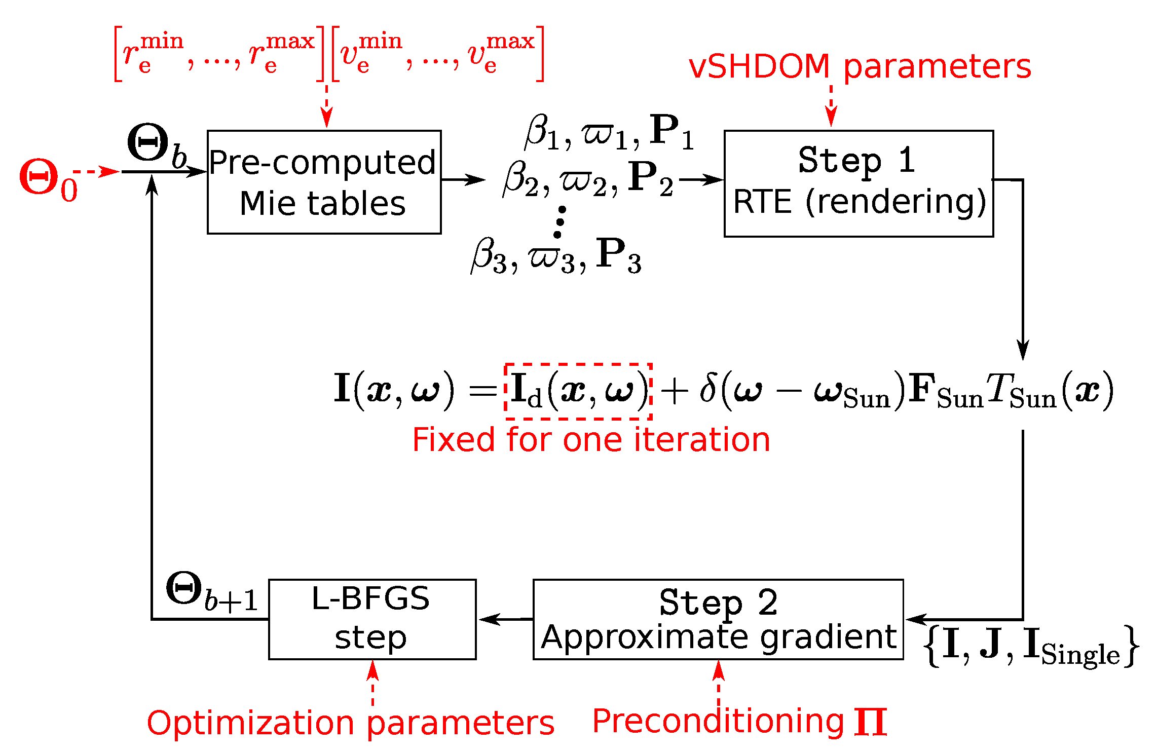
3.3. Iterative Solution Approach

We formulate an iterative algorithm which alternates between two steps (See the diagram in Figure 7).

Starting with an initial guess, ${\Theta }_0$, Step 1 uses vSHDOM to compute the forward (recursive) RT equations. This renders synthetic images according to the multi-view geometry, spectral bands and spatial samples of the cameras. Keeping ${\mathbf{I}}_{\mathrm{d}}$ fixed, Step 2 efficiently computes an approximate gradient with respect to $\Theta$. The approximate gradient is fed into an L-BFGS step to update the current estimate ${\Theta }_b$.

Step 1: RTE Forward Model

The first step in the estimation approach is running the forward model in Equations (8) and (9) using a numerical RTE solver. This requires transforming microphysical to optical properties at every voxel (g) and spectral band ($\lambda$):

$$\mathrm{LWC}\left[g\right],r_{\mathrm{e}}\left[g\right],v_{\mathrm{e}}\left[g\right]⟶{\beta }_{\lambda }\left[g\right],{\varpi }_{\lambda }\left[g\right],{\mathbf{P}}_{\lambda }\left[g\right].$$

(30)

This transformation can be implemented as described in Appendix A, using specifically Equations (A8)–(A13). However, using this implementation during each optimization iteration can be time-consuming. Therefore, we use pre-computed lookup tables, ${\tilde{\sigma }}_{\lambda }\left(r_{\mathrm{e}},v_{\mathrm{e}}\right),{\varpi }_{\lambda }\left(r_{\mathrm{e}},v_{\mathrm{e}}\right),{\mathbf{P}}_{\lambda }\left(r_{\mathrm{e}},v_{\mathrm{e}}\right)$, over the grids $r_{\mathrm{e}}\in \left[r_{\mathrm{e}}^{\min },\dots ,r_{\mathrm{e}}^{\max }\right]$ and $v_{\mathrm{e}}\in \left[v_{\mathrm{e}}^{\min },\dots ,v_{\mathrm{e}}^{\max }\right]$. With these pre-computed tables and $\{\mathrm{LWC}\left[g\right],r_{\mathrm{e}}\left[g\right],v_{\mathrm{e}}\left[g\right]\}$, vSHDOM [60] renders the Stokes vector at each 3D voxel and direction. This is the forward modeling procedure. The result is the set of fields $\mathbf{I}\left(x,\mathbf{\omega }\right),{\mathbf{I}}_{\mathrm{d}}\left(x,\mathbf{\omega }\right),\mathbf{J}\left(x,\mathbf{\omega }\right),{\mathbf{I}}_{\mathrm{Single}}\left(x_{\mathrm{Sun}}\to x^{\prime }\to x_k\right)$.

Step 2: Approximate Jacobian Computation

The forward vRTE model in (11) depends on optical properties $\left(\beta ,\varpi ,\mathbf{P}\right)$, which themselves depend on the sought microphysics. The Jacobian at voxel g is expressed by applying the chain-rule to (11). For example, the derivative with respect to the effective radius is

$$\frac{\partial \mathbf{I}\left[k\right]}{\partial r_{\mathrm{e}}\left[g\right]}=\frac{\partial \mathbf{I}\left[k\right]}{\partial \beta \left[g\right]}\frac{\partial \beta \left[g\right]}{\partial r_{\mathrm{e}}\left[g\right]}+\frac{\partial \mathbf{I}\left[k\right]}{\partial \varpi \left[g\right]}\frac{\partial \varpi \left[g\right]}{\partial r_{\mathrm{e}}\left[g\right]}+\frac{\partial \mathbf{I}\left[k\right]}{\partial \mathbf{P}\left[g\right]}\frac{\partial \mathbf{P}\left[g\right]}{\partial r_{\mathrm{e}}\left[g\right]}.$$

(31)

Analogously, replacing $r_{\mathrm{e}}$ in (31) with $\mathrm{LWC}$ or $v_{\mathrm{e}}$ yields the respective microphysical derivatives. We proceed by expressing the derivatives $\partial \{\beta ,\varpi ,\mathbf{P}\}/\partial \{\mathrm{LWC},r_{\mathrm{e}},v_{\mathrm{e}}\}$. Afterwards, we expand and combine the derivatives $\partial \mathbf{I}/\partial \{\beta ,\varpi ,\mathbf{P}\}$ to express (31).

For each voxel, the derivatives of $\left(\beta ,\varpi ,\mathbf{P}\right)$ with respect to the microphysics are calculated using pre-computed tables

$$\begin{array}{c}\hfill \frac{\partial \beta }{\partial \mathrm{LWC}}=\tilde{\sigma }(r_{\mathrm{e}},v_{\mathrm{e}}),\frac{\partial \beta }{\partial r_{\mathrm{e}}}=\frac{\tilde{\sigma }(r_{\mathrm{e}}+{\epsilon }_{r_{\mathrm{e}}},v_{\mathrm{e}})-\tilde{\sigma }(r_{\mathrm{e}},v_{\mathrm{e}})}{{\epsilon }_{r_{\mathrm{e}}}},\end{array}$$

(32)

$$\begin{array}{c}\hfill \frac{\partial \varpi }{\partial \mathrm{LWC}}=0,\frac{\partial \varpi }{\partial r_{\mathrm{e}}}=\frac{\varpi (r_{\mathrm{e}}+{\epsilon }_{r_{\mathrm{e}}},v_{\mathrm{e}})-\varpi (r_{\mathrm{e}},v_{\mathrm{e}})}{{\epsilon }_{r_{\mathrm{e}}}},\end{array}$$

(33)

$$\begin{array}{c}\hfill \frac{\partial \mathbf{P}}{\partial \mathrm{LWC}}=0,\frac{\partial \mathbf{P}}{\partial r_{\mathrm{e}}}=\frac{\mathbf{P}(r_{\mathrm{e}}+{\epsilon }_{r_{\mathrm{e}}},v_{\mathrm{e}})-\mathbf{P}(r_{\mathrm{e}},v_{\mathrm{e}})}{{\epsilon }_{r_{\mathrm{e}}}},\end{array}$$

(34)

where $v_{\mathrm{e}}$ derivatives are computed analogously to the $r_{\mathrm{e}}$ derivatives. Using the shorthand notation ${\partial }_g\equiv \{\frac{\partial }{\partial \mathrm{LWC}\left[g\right]},\frac{\partial }{\partial r_{\mathrm{e}}\left[g\right]},\frac{\partial }{\partial v_{\mathrm{e}}\left[g\right]}\}$, the overall Jacobian is given by a sum of terms

$${\partial }_g\mathbf{I}\left[k\right]=A_1+A_2+A_3+A_4+A_5+A_6.$$

(35)

The full expression for each term in Equation (35) is given in Appendix B. For example,

$$A_1=-{\ell }_g\left(x_0\to x_k\right)\mathbf{I}\left(x_0,{\mathbf{\omega }}_k\right)T\left(x_0\to x_k\right)\left[{\partial }_g\beta \right].$$

(36)

Let us focus on the term

$$\begin{array}{ccc}\hfill A_4& =& {\int }_{x_0}^{x_k}\left\{\frac{\varpi \left(x^{\prime }\right)}{4\pi }{\int }_{4\pi }\mathbf{P}\left(x^{\prime },{\mathbf{\omega }}_k·{\mathbf{\omega }}^{\prime }\right)\left[{\partial }_g\mathbf{I}\left(x^{\prime },{\mathbf{\omega }}^{\prime }\right)\right]\mathrm{d}{\mathbf{\omega }}^{\prime }\right\}\beta \left(x^{\prime }\right)T\left(x^{\prime }\to x_k\right)\mathrm{d}{x}^{\prime }.\hfill \end{array}$$

(37)

This Jacobian term stands out, because it is the only term which requires computing the derivative of $\mathbf{I}$. This derivative is computationally expensive because $\mathbf{I}$ is computed recursively through the RTE (Equations (8) and (9)). In principle, a change in the microphysics of one voxel can recursively affect the radiance at every other voxel. We decompose ${\partial }_g\mathbf{I}$ using the diffuse-direct decomposition of (12)

$$\begin{array}{c}\hfill {\partial }_g\mathbf{I}\left(x^{\prime },{\mathbf{\omega }}^{\prime }\right)={\partial }_g{\mathbf{I}}_{\mathrm{d}}\left(x^{\prime },{\mathbf{\omega }}^{\prime }\right)+\delta \left({\mathbf{\omega }}^{\prime }-{\mathbf{\omega }}_{\mathrm{Sun}}\right){\mathbf{F}}_{\mathrm{Sun}}\left[{\partial }_{g}T\left(x_{\mathrm{Sun}}\to x^{\prime }\right)\right].\end{array}$$

(38)

At the core our approach for computational efficiency is the assumption that the diffuse light ${\mathbf{I}}_{\mathrm{d}}$ is less sensitive to slight changes in the microphysical properties of any single voxel g. Rather, ${\mathbf{I}}_{\mathrm{d}}$ is impacted mainly by bulk changes to the over-all volume. Thus, we approximate (37) by keeping ${\mathbf{I}}_{\mathrm{d}}$ independent of $\Theta$ for a single iteration of the gradient computation, that is,

$${\partial }_g{\mathbf{I}}_{\mathrm{d}}\approx 0.$$

(39)

This bypasses the complexity of recursively computing ${\partial }_g{\mathbf{I}}_{\mathrm{d}}$.

It is important to note that at every iteration, the Jacobian ${\nabla }_{\Theta }\mathbf{I}\left[k\right]$ still is impacted by ${\mathbf{I}}_{\mathrm{d}}$. This is because ${\mathbf{I}}_{\mathrm{d}}$ affects $\mathbf{I}$ through Equation (12), and $\mathbf{I}$ appears in the terms $A_1,\dots ,A_6$. As the estimated medium properties evolve through iterations, so does ${\mathbf{I}}_{\mathrm{d}}$ (in Step 1, above). We just assume during Step 2 that ${\partial }_g{\mathbf{I}}_{\mathrm{d}}$ is negligible compared to other terms in Equation (35).

Contrary to ${\mathbf{I}}_{\mathrm{d}}$, the single-scattered component is highly sensitive to changes in the micro-physical properties of a single voxel. We therefore include an exact treatment of single-scattering in the gradient computation (Appendix B). This is the essence of our numerical optimization approach. It enables tackling multiple-scattering tomography, in practice. Simulation results presented in the following section rely on additional numerical considerations (e.g., initialization, preconditioning, convergence criteria), which are all described in the accompanying Appendix D.

4. Computational Efficiency

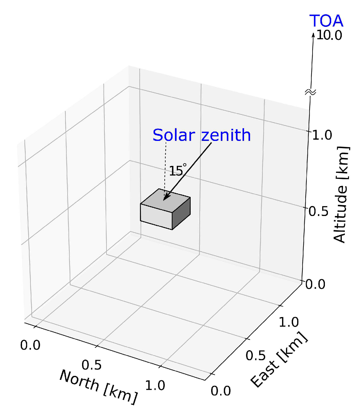
Section 3.2 and Section 3.3 describe our iterative gradient-based approach to Equations (28) and (29). The approach relies on an approximate Jacobian. We argue that our gradient computation is efficient, relative to the state of the art. Recall that the goal is estimation of three unknown cloud-droplet parameters per voxel. Each Jacobian component expresses differentiation relative to each parameter in each voxel. Accounting for the need to run the forward model in Equation (28) and the Jacobian, brute force computation requires $3N_{\mathrm{grid}}+1$ full 3D vRTE computations, for each iteration of the optimization.

An alternative tractable approach relies on adjoint differentiation of 3D vRTE. To the best of our knowledge, only Martin et al. [75] have at least formulated a potentially efficient atmosphere/surface tomography based on the adjoint 3D vector RTE. However, the method was only demonstrated using 2D scalar RT, showing promise in retrieving cloud extinction [76]. The adjoint approach requires computing one full 3D vRTE and one full adjoint-3D vRTE, per gradient computation. Due to symmetry, the overall complexity of each iteration of the optimization would be that of two 3D-vRTE computations.

Our method to approximate the gradient per iteration requires lower resources: one forward full 3D vRTE (for Equation (28)) computation and a simple single-scattering computation. Intuitively, our approach compromises gradient accuracy at voxels where the adjoint Stokes vector has undergone multiple scattering events. These voxels will tend to be at larger optical distances from the sensors. The scattering events cause a decorrelation of the adjoint Stokes vector from the optical properties and therefore loss of sensitivity to the properties of individual voxels. The measurement sensitivity to cloud properties is therefore expected to diminish. Thus, while the accuracy of the gradient in these voxels is reduced, so is the magnitude of the gradient. This region of diminished sensitivity coincides with the “hidden core” of the cloud. We refer the reader to Forster et al. [77] for more details on the hidden core concept.

5. Simulations

In the context of tomography, simultaneity is defined by the evolution timescales of targeted clouds and by the time it takes to acquire multi-angular data. Becasue updraft timescales of shallow cumulus are $\sim 15min$ [78], our target clouds significantly evolve over a typical single-platform observation time span (e.g., 7 min for Terra’s MISR). Hence, single-platform systems do not satisfy simultaneity in out context. As mentioned, real data of simultaneous spaceborne multi-angular polarimetric images of clouds does not yet exist, but a mission to supply this data is in the works. Therefore, we use careful simulations to test the approach. We simulate an atmosphere with molecular Rayleigh scattering and liquid water clouds. Rayleigh scattering is calculated from the Air Force Geophysics Laboratory (AFGL) database [79] for a summer mid-latitude atmosphere. Mie tables are pre-computed for $r_{\mathrm{e}}\in [4,25]\mathsf{\mu }$m and $v_{\mathrm{e}}=0.1$ with $N_{r_{\mathrm{e}}}=100$. The surface is Lambertian with a water-like albedo of $0.05$. For realistic complexity, a Large Eddy Simulation (LES) model [80] was used to generate a cloud field. Each voxel is of size 20 × 20 × 40 m${}^3$. The LES outputs [80] are clouds with 3D variable $\mathrm{LWC}$ and 1D (vertically) variable $r_{\mathrm{e}}$. A typical value [81] of $v_{\mathrm{e}}=0.1$ was chosen. Consequently, the present recovery demonstrations recover $\mathrm{LWC}$ and $r_{\mathrm{e}}$ on their respective native LES grid. On the other hand, $v_{\mathrm{e}}=0.1$ is excluded from the unknowns. The assumption of fixed $v_{\mathrm{e}}$ is not fundamental to our approach or implementation, however, relaxing this assumption warrants an investigation which will be done in future work. The spatial variability of the recovered parameters is discussed in more detail in Section 6.

From the generated cloud field, two isolated cloudy regions are taken for reconstruction:

• Scene A: An atmospheric domain of dimensions 0.64 × 0.72 × 20 km${}^3$ with an isolated cloud (see synthetic AirMSPI nadir view in Figure 8).
• Scene B: An atmospheric domain of dimensions 2.42 × 2.1 × 8 km${}^3$ with several clouds of varying optical thickness (see synthetic AirMSPI nadir view in Figure 9).

Synthetic measurements rendered with the spatial resolution and angular sampling of AirMSPI [14], namely, 10 m pixels and 9 viewing angles: $\pm {70.5}^{°}$, $\pm {60}^{°}$, $\pm {45.6}^{°}$, $\pm {26.1}^{°}$, and $0^{°}$ from zenith, where ± indicates fore- and aft-views along the northbound flight path. The solar zenith angle is ${15}^{°}$ from nadir in the measurement plane, that is, $0^{°}$ solar azimuth. We simulate measurements at AirMSPI’s three polarized spectral bands: $\lambda =\left[0.47,0.66,0.865\right]\mathsf{\mu }$m. The bandwidths are narrow enough (≈46 nm) to render images using a single representative wavelength per band.

Single scattering albedos for these wavelengths equal unity (up to 4 significant digits). In other words, and in sharp contrast with the operational Nakajima–King [9] two-wavelengths non-tomographic retrieval, absorption by droplets plays no role in this demonstration of the tomography of cloud microphysics. The measurements are synthesized with realistic noise, according to the AirMSPI data acquisition model (see Appendix C).

Qualitative volumetric results of the recovered LWC for Scene A are shown in Figure 10. Scatter plot of the recovered LWC and the recovery results of $r_{\mathrm{e}}$ for Scene A are given in Figure 11. Qualitative volumetric results of the recovered LWC for Scene B are shown in Figure 12. A scatter plot of the recovered LWC and the recovery results of $r_{\mathrm{e}}$ for Scene B are given in Figure 13.

For quantitative assessment of the recovery, we use local mean error $ϵ$, and global bias measures [53] $\vartheta$:

$$\begin{array}{c}\hfill {ϵ}_{\mathrm{LWC}}=\frac{\parallel \widehat{\mathrm{LWC}}{-\mathrm{LWC}\parallel }_1}{{\parallel \mathrm{LWC}\parallel }_1},{\vartheta }_{\mathrm{LWC}}=\frac{\parallel \widehat{\mathrm{LWC}}{\parallel }_1-{\parallel \mathrm{LWC}\parallel }_1}{{\parallel \mathrm{LWC}\parallel }_1},{ϵ}_{r_{\mathrm{e}}}=\frac{\parallel \widehat{r_{\mathrm{e}}}-r_{\mathrm{e}}{\parallel }_1}{\parallel r_{\mathrm{e}}{\parallel }_1}.\end{array}$$

(40)

We further define the Root Mean Square (RMS) error and bias of the retrieved LWC as:

$$\mathrm{RMS}=\frac{1}{\sqrt{N_{\mathrm{grid}}}}{\parallel \widehat{\mathrm{LWC}}-\mathrm{LWC}\parallel }_2^1,\mathrm{bias}=\frac{1}{N_{\mathrm{grid}}}\sum _{g=1}^{N_{\mathrm{grid}}}(\widehat{\mathrm{LWC}}\left[g\right]-\overline{\mathrm{LWC}}\left[g\right]).$$

(41)

The quantitative error measures upon convergence for the two scenes are:

  Scene A: ${ϵ}_{r_{\mathrm{e}}}\approx 11\%,{ϵ}_{\mathrm{LWC}}\approx 30\%,{\vartheta }_{\mathrm{LWC}}\approx -4\%,\begin{array}{c}\hfill \mathrm{RMS}\approx 0.065g/m^3,\mathrm{bias}\approx -0.002g/m^3\end{array}$,

  Scene B: ${ϵ}_{r_{\mathrm{e}}}\approx 13\%,{ϵ}_{\mathrm{LWC}}\approx 29\%,{\vartheta }_{\mathrm{LWC}}\approx -5\%,\begin{array}{c}\hfill \mathrm{RMS}\approx 0.085g/m^3,\mathrm{bias}\approx -0.0035g/m^3\end{array}$.

Using a 2.50 GHz CPU, the recovery run-time of cloud properties in Scenes A,B was $\sim 13$ h and $\sim 10$ days, respectively.

Multi-angular tomographic retrieval enables vertical resolution of the droplet effective radius. By contrast, a homogeneous droplet radius is typically retrieved by mono-angular observations fitted to a plane-parallel homogeneous cloud model. The retrieval errors of droplet radii in the demonstrations above are significantly smaller than retrieval errors of a homogeneous droplet radius. The latter can easily exceed 50% in similar conditions to our study that is, shallow cumuli and illumination conditions (see e.g., Reference [82]).

6. Discussion

In the formulation of our retrieval, and in nature, the droplet effective radius $r_{\mathrm{e}}$ and droplet effective variance $v_{\mathrm{e}}$ vary in 3D. This allows us to, in principle, localize the variations in cloud microphysical properties which is a significant advance over other methods. Operational remote sensing algorithms, which rely on 1D RT and plane-parallel cloud models, retrieve a single value for $r_{\mathrm{e}}$ (and for $v_{\mathrm{e}}$), for each cloudy pixel. This occurs both in bi-spectral [9,83] and polarimetric [11,84] techniques. The physical interpretation is complicated by the difficulty in determining which portion of the cloud the retrieved quantities corresponds to.

In our current demonstrations we assume 1D variable $r_{\mathrm{e}}$ and a completely homogeneous $v_{\mathrm{e}}$. This is much more general than operational methods, but still a degenerate representation compared to full 3D variability. We now discuss the realism of such a representation.

Vertically varying droplet size distributions arise as a result of moist adiabatic thermodynamics in vertically stratified environments (e.g., Reference [81]). Further 3D variability forms due to the diabatic mixing of air parcels in the turbulent processes of entrainment and detrainment. Despite the complexity of these processes, there is evidence that the horizontal variability $r_{\mathrm{e}}$ is indeed small over a cloud scale.

This evidence comes from in-situ aircraft observations of shallow cumulus [85,86,87], modelling studies [88] and theory [89]. However, there are also select observations of monsoonal clouds [90] and theoretical arguments [89] that suggest there is a sharp gradient in the droplet effective radius in the very outer shell of the clouds. If this is the case, then a representation having vertical-only variation of $r_{\mathrm{e}}$ loses validity at the outer shell.

The value of $v_{\mathrm{e}}$ can also vary significantly across different environmental conditions. This is seen in research flights including in-situ measurements [91,92,93,94,95]. Moreover, in LES simulations of shallow cumulus clouds with bin microphysics, $v_{\mathrm{e}}$ might range from 0.01 to 0.26 [96]. The core of a cloud tends to have a low effective variance as condensation is the dominant process there [96,97]. Cloud edges, in contrast, experience also evaporation and entrainment mixing, as the cloud is diluted by environmental air [98]. This tends to increase $v_{\mathrm{e}}$. If the cloud has precipitation, spatial variability of $v_{\mathrm{e}}$ increases [99].

While horizontal variations reduce the accuracy of our demonstrated retrieval, these points show that the approximations used in our demonstrations are often reasonable and a significant advance. To further push the potential of the general framework proposed here and retrieve additional degrees of freedom describing microphysical variations in 3D, we may include more information. One option is to include additional measurements, for example, by using a combination of AirMSPI [14] and Research Spectro-Polarimeter (RSP) [100]. Another option is to introduce regularization schemes, which mathematically express the natural trends of horizontal variability mentioned above. The 3D tomographic approach presented in the paper offers a lot more flexibility than current operational analyses and enables the development and application of retrievals that might provide new insight into cloud microphysics.

7. Summary & Outlook

We derive the tomography of cloud microphysics based on multi-view/multi-spectral polarimetric measurements of scattered sunlight. This novel type of tomography uses, for the first time, 3D polarized RT as the image formation model. The recovery of droplet sizes is made possible due to the crucial phase-function information carried by the polarized signal. We define a model-fitting error function and compute approximate gradients of this function to make the recovery tractable. Demonstration are done on synthetic 3D clouds, based on a Large Eddy Simulation with the effective radius assumed to vary only vertically. Our open-source code is publicly available [101].

Future work will address the extent to which polarimetric measurements penetrate the cloud and the relation between $r_{\mathrm{e}}$ in the outer shell and $r_{\mathrm{e}}$ in the cloud core, as defined by Forster et al. [77]. Furthermore, we will relax the fixed $v_{\mathrm{e}}$ assumption that was used in the demonstrations, and thus assess full microphysical retrieval capabilities of polarization measurements. Moreover, future plans include experimental demonstration and use, while the CloudCT formation orbits. Research is ongoing [77] about the adaptation of our cloud tomography methodology for satellite data as can be obtained from the multi-view imaging from MISR on Terra and a SWIR view from the collocated MODIS, but with significantly lower spatial resolution than used so far.

Lastly, we note that our atmospheric tomography approach described herein can be adapted to aerosols, including dense plumes of wild fire smoke, volcanic ash, and dust near their sources. The main difference in this extended application is that the forward model must be further linearized with respect to the complex refractive index of the varying aerosol material, which has been done for 1D polarized RT (e.g., Reference [102]), even for non-sphericity effects (e.g., Reference [103]).

References

1. Trenberth, K.E.; Fasullo, J.T.; Kiehl, J. Earth’s global energy budget. Bull. Am. Meteorol. Soc. 2009, 90, 311–324. [Google Scholar] [CrossRef]
2. Boucher, O.; Randall, D.; Artaxo, P.; Bretherton, C.; Feingold, G.; Forster, P.; Kerminen, V.M.; Kondo, Y.; Liao, H.; Lohmann, U.; et al. Clouds and aerosols. In Climate Change 2013: The Physical Science Basis. Contribution of Working Group I to the Fifth Assessment Report of the Intergovernmental Panel on Climate Change; Cambridge University Press: Cambridge, UK, 2013; pp. 571–657. [Google Scholar]
3. Rosenfeld, D.; Lensky, I.M. Satellite-based insights into precipitation formation processes in continental and maritime convective clouds. Bull. Am. Meteorol. Soc. 1998, 79, 2457–2476. [Google Scholar] [CrossRef] [Green Version]
4. Platnick, S.; King, M.; Ackerman, S.; Menzel, W.; Baum, B.; Riedi, J.; Frey, R. The MODIS cloud products: Algorithms and examples from Terra. IEEE Trans. Geosci. Remote Sens. 2003, 41, 459–473. [Google Scholar] [CrossRef] [Green Version]
5. Marshak, A.; Platnick, S.; Várnai, T.; Wen, G.; Cahalan, R.F. Impact of three-dimensional radiative effects on satellite retrievals of cloud droplet sizes. J. Geophys. Res. Atmos. 2006, 111. [Google Scholar] [CrossRef]
6. Cho, H.M.; Zhang, Z.; Meyer, K.; Lebsock, M.; Platnick, S.; Ackerman, A.S.; Di Girolamo, L.; C.-Labonnote, L.; Cornet, C.; Riedi, J.; et al. Frequency and causes of failed MODIS cloud property retrievals for liquid phase clouds over global oceans. J. Geophys. Res. Atmos. 2015, 120, 4132–4154. [Google Scholar] [CrossRef]
7. National Academies of Sciences, Engineering, and Medicine. Thriving on Our Changing Planet: A Decadal Strategy for Earth Observation from Space; The National Academies Press: Washington, DC, USA, 2018. [Google Scholar]
8. Schilling, K.; Schechner, Y.Y.; Koren, I. CloudCT—computed tomography of clouds by a small satellite formation. In Proceedings of the IAA Symposium on Small Satellites for Earth Observation, Berlin, Germany, 6–10 May 2019. [Google Scholar]
9. Nakajima, T.; King, M.D. Determination of the optical thickness and effective particle radius of clouds from reflected solar radiation measurements. Part I: Theory. J. Atmos. Sci. 1990, 47, 1878–1893. [Google Scholar] [CrossRef] [Green Version]
10. Deschamps, P.Y.; Bréon, F.M.; Leroy, M.; Podaire, A.; Bricaud, A.; Buriez, J.C.; Seze, G. The POLDER mission: Instrument characteristics and scientific objectives. IEEE Trans. Geosci. Remote. Sens. 1994, 32, 598–615. [Google Scholar] [CrossRef]
11. Bréon, F.M.; Goloub, P. Cloud droplet effective radius from spaceborne polarization measurements. Geophys. Res. Lett. 1998, 25, 1879–1882. [Google Scholar] [CrossRef]
12. Kalashnikova, O.V.; Garay, M.J.; Davis, A.B.; Diner, D.J.; Martonchik, J.V. Sensitivity of multi-angle photo-polarimetry to vertical layering and mixing of absorbing aerosols: Quantifying measurement uncertainties. J. Quant. Spectrosc. Radiat. Transf. 2011, 112, 2149–2163. [Google Scholar] [CrossRef]
13. Lukashin, C.; Wielicki, B.A.; Young, D.F.; Thome, K.; Jin, Z.; Sun, W. Uncertainty estimates for imager reference inter-calibration with CLARREO reflected solar spectrometer. IEEE Trans. Geosci. Remote. Sens. 2013, 51, 1425–1436. [Google Scholar] [CrossRef]
14. Diner, D.; Xu, F.; Garay, M.; Martonchik, J.; Rheingans, B.; Geier, S.; Davis, A.; Hancock, B.; Jovanovic, V.; Bull, M.; et al. The Airborne Multiangle SpectroPolarimetric Imager (AirMSPI): A new tool for aerosol and cloud remote sensing. Atmos. Meas. Tech. 2013, 6, 2007–2025. [Google Scholar] [CrossRef] [Green Version]
15. Diner, D.J.; Boland, S.W.; Brauer, M.; Bruegge, C.; Burke, K.A.; Chipman, R.; Di Girolamo, L.; Garay, M.J.; Hasheminassab, S.; Hyer, E.; et al. Advances in multiangle satellite remote sensing of speciated airborne particulate matter and association with adverse health effects: From MISR to MAIA. J. Appl. Remote. Sens. 2018, 12, 042603. [Google Scholar] [CrossRef] [Green Version]
16. Martins, J.V.; Nielsen, T.; Fish, C.; Sparr, L.; Fernandez-Borda, R.; Schoeberl, M.; Remer, L. HARP CubeSat–An innovative hyperangular imaging polarimeter for earth science applications. In Proceedings of the Small Sat Pre-Conference Workshop, Logan, UT, USA, 3 August 2014; Volume 20. [Google Scholar]
17. Emde, C.; Barlakas, V.; Cornet, C.; Evans, F.; Korkin, S.; Ota, Y.; Labonnote, L.C.; Lyapustin, A.; Macke, A.; Mayer, B.; et al. IPRT polarized radiative transfer model intercomparison project—Phase A. J. Quant. Spectrosc. Radiat. Transf. 2015, 164, 8–36. [Google Scholar] [CrossRef] [Green Version]
18. Emde, C.; Barlakas, V.; Cornet, C.; Evans, F.; Wang, Z.; Labonotte, L.C.; Macke, A.; Mayer, B.; Wendisch, M. IPRT polarized radiative transfer model intercomparison project—Three-dimensional test cases (Phase B). J. Quant. Spectrosc. Radiat. Transf. 2018, 209, 19–44. [Google Scholar] [CrossRef] [Green Version]
19. Kak, A.; Slaney, M. Principles of Computerized Tomographic Imaging IEEE Press; IEEE Press: Piscataway, NJ, USA, 1988. [Google Scholar]
20. Gordon, R.; Bender, R.; Herman, G.T. Algebraic reconstruction techniques (ART) for three-dimensional electron microscopy and X-ray photography. J. Theor. Biol. 1970, 29, 471–481. [Google Scholar] [CrossRef]
21. Marshak, A.; Davis, A.; Cahalan, R.; Wiscombe, W. Nonlocal independent pixel approximation: Direct and inverse problems. IEEE Trans. Geosci. Remote. Sens. 1998, 36, 192–204. [Google Scholar] [CrossRef] [Green Version]
22. Faure, T.; Isaka, H.; Guillemet, B. Neural network retrieval of cloud parameters of inhomogeneous and fractional clouds: Feasibility study. Remote Sens. Environ. 2001, 77, 123–138. [Google Scholar] [CrossRef]
23. Faure, T.; Isaka, H.; Guillemet, B. Neural network retrieval of cloud parameters from high-resolution multispectral radiometric data: A feasibility study. Remote Sens. Environ. 2002, 80, 285–296. [Google Scholar] [CrossRef]
24. Cornet, C.; Isaka, H.; Guillemet, B.; Szczap, F. Neural network retrieval of cloud parameters of inhomogeneous clouds from multispectral and multiscale radiance data: Feasibility study. J. Geophys. Res. Atmos. 2004, 109, D12203. [Google Scholar] [CrossRef]
25. Zinner, T.; Mayer, B.; Schröder, M. Determination of three-dimensional cloud structures from high-resolution radiance data. J. Geophys. Res. Atmos. 2006, 111, D08204. [Google Scholar] [CrossRef]
26. Iwabuchi, H.; Hayasaka, T. A multi-spectral non-local method for retrieval of boundary layer cloud properties from optical remote sensing data. Remote Sens. Environ. 2003, 88, 294–308. [Google Scholar] [CrossRef]
27. Diner, D.J.; Beckert, J.C.; Reilly, T.H.; Bruegge, C.J.; Conel, J.E.; Kahn, R.A.; Martonchik, J.V.; Ackerman, T.P.; Davies, R.; Gerstl, S.A.W.; et al. Multi-angle Imaging SpectroRadiometer (MISR) instrument description and experiment overview. IEEE Trans. Geosci. Remote Sens. 1998, 36, 1072–1087. [Google Scholar] [CrossRef]
28. Marchand, R.; Ackerman, T. Evaluation of radiometric measurements from the NASA Multiangle Imaging SpectroRadiometer (MISR): Two-and three-dimensional radiative transfer modeling of an inhomogeneous stratocumulus cloud deck. J. Geophys. Res. Atmos. 2004, 109. [Google Scholar] [CrossRef]
29. Seiz, G.; Davies, R. Reconstruction of cloud geometry from multi-view satellite images. Remote. Sens. Environ. 2006, 100, 143–149. [Google Scholar] [CrossRef]
30. Cornet, C.; Davies, R. Use of MISR measurements to study the radiative transfer of an isolated convective cloud: Implications for cloud optical thickness retrieval. J. Geophys. Res. Atmos. 2008, 113. [Google Scholar] [CrossRef]
31. Evans, K.F.; Marshak, A.; Várnai, T. The Potential for Improved Boundary Layer Cloud Optical Depth Retrievals from the Multiple Directions of MISR. J. Atmos. Sci. 2008, 65, 3179–3196. [Google Scholar] [CrossRef]
32. Romps, D.M.; Öktem, R. Observing Clouds in 4D with Multiview Stereophotogrammetry. Bull. Am. Meteorol. Soc. 2018, 99, 2575–2586. [Google Scholar] [CrossRef] [Green Version]
33. Castro, E.; Ishida, T.; Takahashi, Y.; Kubota, H.; Perez, G.J.; Marciano, J.S. Determination of cloud-top Height through three-dimensional cloud Reconstruction using DIWATA-1 Data. Sci. Rep. 2020, 10, 1–13. [Google Scholar] [CrossRef]
34. Alexandrov, M.D.; Cairns, B.; Emde, C.; Ackerman, A.S.; Ottaviani, M.; Wasilewski, A.P. Derivation of cumulus cloud dimensions and shape from the airborne measurements by the Research Scanning Polarimeter. Remote Sens. Environ. 2016, 177, 144–152. [Google Scholar] [CrossRef]
35. Lee, B.; Di Girolamo, L.; Zhao, G.; Zhan, Y. Three-Dimensional Cloud Volume Reconstruction from the Multi-angle Imaging SpectroRadiometer. Remote Sens. 2018, 10, 1858. [Google Scholar] [CrossRef] [Green Version]
36. Yu, H.; Ma, J.; Ahmad, S.; Sun, E.; Li, C.; Li, Z.; Hong, J. Three-Dimensional Cloud Structure Reconstruction from the Directional Polarimetric Camera. Remote Sens. 2019, 11, 2894. [Google Scholar] [CrossRef] [Green Version]
37. Veikherman, D.; Aides, A.; Schechner, Y.Y.; Levis, A. Clouds in The Cloud. In Proceedings of the Asian Conference on Computer Vision (ACCV), Singapore, 1–5 November 2014; pp. 659–674. [Google Scholar]
38. Zinner, T.; Marshak, A.; Lang, S.; Martins, J.V.; Mayer, B. Remote sensing of cloud sides of deep convection: Towards a three-dimensional retrieval of cloud particle size profiles. Atmos. Chem. Phys. 2008, 8, 4741–4757. [Google Scholar] [CrossRef] [Green Version]
39. Alexandrov, M.D.; Miller, D.J.; Rajapakshe, C.; Fridlind, A.; van Diedenhoven, B.; Cairns, B.; Ackerman, A.S.; Zhang, Z. Vertical profiles of droplet size distributions derived from cloud-side observations by the research scanning polarimeter: Tests on simulated data. Atmos. Res. 2020, 239, 104924. [Google Scholar] [CrossRef] [PubMed]
40. Okamura, R.; Iwabuchi, H.; Schmidt, K.S. Feasibility study of multi-pixel retrieval of optical thickness and droplet effective radius of inhomogeneous clouds using deep learning. Atmos. Meas. Tech. 2017, 10, 4747–4759. [Google Scholar] [CrossRef] [Green Version]
41. Masuda, R.; Iwabuchi, H.; Schmidt, K.S.; Damiani, A.; Kudo, R. Retrieval of Cloud Optical Thickness from Sky-View Camera Images using a Deep Convolutional Neural Network based on Three-Dimensional Radiative Transfer. Remote Sens. 2019, 11, 1962. [Google Scholar] [CrossRef] [Green Version]
42. Liou, K.N.; Ou, S.C.; Takano, Y.; Roskovensky, J.; Mace, G.G.; Sassen, K.; Poellot, M. Remote sensing of three-dimensional inhomogeneous cirrus clouds using satellite and mm-wave cloud radar data. Geophys. Res. Lett. 2002, 29, 1360. [Google Scholar] [CrossRef] [Green Version]
43. Barker, H.; Jerg, M.; Wehr, T.; Kato, S.; Donovan, D.; Hogan, R. A 3D cloud-construction algorithm for the EarthCARE satellite mission. Q. J. R. Meteorol. Soc. 2011, 137, 1042–1058. [Google Scholar] [CrossRef] [Green Version]
44. Fielding, M.D.; Chiu, J.C.; Hogan, R.J.; Feingold, G. A novel ensemble method for retrieving properties of warm cloud in 3-D using ground-based scanning radar and zenith radiances. J. Geophys. Res. Atmos. 2014, 119, 10–912. [Google Scholar] [CrossRef] [Green Version]
45. Hasmonay, R.A.; Yost, M.G.; Wu, C.F. Computed tomography of air pollutants using radial scanning path-integrated optical remote sensing. Atmos. Environ. 1999, 33, 267–274. [Google Scholar] [CrossRef]
46. Todd, L.A.; Ramanathan, M.; Mottus, K.; Katz, R.; Dodson, A.; Mihlan, G. Measuring chemical emissions using an open-path Fourier transform infrared (OP-FTIR) spectroscopy and computer-assisted tomography. Atmos. Environ. 2001, 35, 1937–1947. [Google Scholar] [CrossRef]
47. Kazahaya, R.; Mori, T.; Kazahaya, K.; Hirabayashi, J. Computed tomography reconstruction of SO2 concentration distribution in the volcanic plume of Miyakejima, Japan, by airborne traverse technique using three UV spectrometers. Geophys. Res. Lett. 2008, 35. [Google Scholar] [CrossRef]
48. Wright, T.E.; Burton, M.; Pyle, D.M.; Caltabiano, T. Scanning tomography of SO2 distribution in a volcanic gas plume. Geophys. Res. Lett. 2008, 35. [Google Scholar] [CrossRef]
49. Warner, J.; Drake, J.; Snider, J. Liquid water distribution obtained from coplanar scanning radiometers. J. Atmos. Ocean. Technol. 1986, 3, 542–546. [Google Scholar] [CrossRef] [Green Version]
50. Huang, D.; Liu, Y.; Wiscombe, W. Determination of cloud liquid water distribution using 3D cloud tomography. J. Geophys. Res. Atmos. 2008, 113. [Google Scholar] [CrossRef]
51. Huang, D.; Liu, Y.; Wiscombe, W. Cloud tomography: Role of constraints and a new algorithm. J. Geophys. Res. Atmos. 2008, 113. [Google Scholar] [CrossRef]
52. Garay, M.J.; Davis, A.B.; Diner, D.J. Tomographic reconstruction of an aerosol plume using passive multiangle observations from the MISR satellite instrument. Geophys. Res. Lett. 2016, 43, 12–590. [Google Scholar] [CrossRef]
53. Aides, A.; Schechner, Y.Y.; Holodovsky, V.; Garay, M.J.; Davis, A.B. Multi-sky-view 3D aerosol distribution recovery. Opt. Express 2013, 21, 25820–25833. [Google Scholar] [CrossRef] [Green Version]
54. Geva, A.; Schechner, Y.Y.; Chernyak, Y.; Gupta, R. X-ray computed tomography through scatter. In Proceedings of the European Conference on Computer Vision (ECCV), Munich, Germany, 8–14 September 2018; pp. 34–50. [Google Scholar]
55. Arridge, S.R. Optical tomography in medical imaging. Inverse Probl. 1999, 15, R41. [Google Scholar] [CrossRef] [Green Version]
56. Boas, D.A.; Brooks, D.H.; Miller, E.L.; DiMarzio, C.A.; Kilmer, M.; Gaudette, R.J.; Zhang, Q. Imaging the body with diffuse optical tomography. IEEE Signal Process. Mag. 2001, 18, 57–75. [Google Scholar] [CrossRef]
57. Arridge, S.R.; Schotland, J.C. Optical tomography: Forward and inverse problems. Inverse Probl. 2009, 25, 123010. [Google Scholar] [CrossRef]
58. Che, C.; Luan, F.; Zhao, S.; Bala, K.; Gkioulekas, I. Inverse transport networks. arXiv 2018, arXiv:1809.10820. [Google Scholar]
59. Evans, K.F. The spherical harmonics discrete ordinate method for three-dimensional atmospheric radiative transfer. J. Atmos. Sci. 1998, 55, 429–446. [Google Scholar] [CrossRef]
60. Doicu, A.; Efremenko, D.; Trautmann, T. A multi-dimensional vector spherical harmonics discrete ordinate method for atmospheric radiative transfer. J. Quant. Spectrosc. Radiat. Transf. 2013, 118, 121–131. [Google Scholar] [CrossRef]
61. Levis, A.; Schechner, Y.Y.; Aides, A.; Davis, A.B. Airborne three-dimensional cloud tomography. In Proceedings of the IEEE International Conference on Computer Vision (ICCV), Santiago, Chile, 7–13 December 2015; pp. 3379–3387. [Google Scholar]
62. Holodovsky, V.; Schechner, Y.Y.; Levin, A.; Levis, A.; Aides, A. In-situ multi-view multi-scattering stochastic tomography. In Proceedings of the IEEE International Conference on Computational Photography (ICCP), Evanston, IL, USA, 13–14 May 2016; pp. 1–12. [Google Scholar]
63. Levis, A.; Schechner, Y.Y.; Davis, A.B. Multiple-scattering microphysics tomography. In Proceedings of the IEEE Conference on Computer Vision and Pattern Recognition (CVPR), Honolulu, HI, USA, 21–26 July 2017; pp. 6740–6749. [Google Scholar]
64. Aides, A.; Levis, A.; Holodovsky, V.; Schechner, Y.Y.; Althausen, D.; Vainiger, A. Distributed Sky Imaging Radiometry and Tomography. In Proceedings of the IEEE International Conference on Computational Photography (ICCP), Saint Louis, MO, USA, 24–26 April 2020; pp. 1–12. [Google Scholar]
65. Loeub, T.; Levis, A.; Holodovsky, V.; Schechner, Y.Y.; Chernyak, Y.; Gupta, R. Monotonicity Prior for Cloud Tomography. In Proceedings of the European Conference on Computer Vision (ECCV), Glasgow, Scotlang, 24–29 August 2020. [Google Scholar]
66. Hansen, J.E. Multiple scattering of polarized light in planetary atmospheres, Part II. Sunlight reflected by terrestrial water clouds. J. Atmos. Sci. 1971, 28, 1400–1426. [Google Scholar] [CrossRef] [Green Version]
67. Marshak, A.; Davis, A. 3D Radiative Transfer in Cloudy Atmospheres; Springer Science & Business Media: Berlin/Heidelberg, Germany, 2005. [Google Scholar]
68. Chylek, P. Extinction and liquid water content of fogs and clouds. J. Atmos. Sci. 1978, 35, 296–300. [Google Scholar]
69. Bohren, C.F.; Huffman, D.R. Absorption and Scattering of Light by Small Particles; John Wiley & Sons: Hoboken, NJ, USA, 2008. [Google Scholar]
70. Chandrasekhar, S. Radiative Transfer; Oxford University Press: Oxford, UK, 1950. [Google Scholar]
71. Mayer, B. Radiative transfer in the cloudy atmosphere. Eur. Phys. J. Conf. 2009, 1, 75–99. [Google Scholar] [CrossRef]
72. Nakajima, T.; Tanaka, M. Algorithms for radiative intensity calculations in moderately thick atmospheres using a truncation approximation. J. Quant. Spectrosc. Radiat. Transf. 1988, 40, 51–69. [Google Scholar] [CrossRef]
73. Zhu, C.; Byrd, R.H.; Lu, P.; Nocedal, J. Algorithm 778: L-BFGS-B: Fortran subroutines for large-scale bound-constrained optimization. ACM Trans. Math. Softw. 1997, 23, 550–560. [Google Scholar] [CrossRef]
74. Doicu, A.; Efremenko, D.S. Linearizations of the Spherical Harmonic Discrete Ordinate Method (SHDOM). Atmosphere 2019, 10, 292. [Google Scholar] [CrossRef] [Green Version]
75. Martin, W.; Cairns, B.; Bal, G. Adjoint methods for adjusting three-dimensional atmosphere and surface properties to fit multi-angle/multi-pixel polarimetric measurements. J. Quant. Spectrosc. Radiat. Transf. 2014, 144, 68–85. [Google Scholar] [CrossRef] [Green Version]
76. Martin, W.G.; Hasekamp, O.P. A demonstration of adjoint methods for multi-dimensional remote sensing of the atmosphere and surface. J. Quant. Spectrosc. Radiat. Transf. 2018, 204, 215–231. [Google Scholar] [CrossRef]
77. Forster, L.; Davis, A.B.; Diner, D.J.; Mayer, B. Toward Cloud Tomography from Space using MISR and MODIS: Locating the “Veiled Core” in Opaque Convective Clouds. arXiv 2019, arXiv:1910.00077. [Google Scholar]
78. Zhao, M.; Austin, P.H. Life cycle of numerically simulated shallow cumulus clouds. Part II: Mixing dynamics. J. Atmos. Sci. 2005, 62, 1291–1310. [Google Scholar] [CrossRef]
79. Anderson, G.P.; Clough, S.A.; Kneizys, F.; Chetwynd, J.H.; Shettle, E.P. AFGL Atmospheric Constituent Profiles (0.120 km); Technical Report; Air Force Geophysics Lab: Hanscom AFB, MA, USA, 1986. [Google Scholar]
80. Matheou, G.; Chung, D. Large-eddy simulation of stratified turbulence. Part 2: Application of the stretched-vortex model to the atmospheric boundary layer. J. Atmos. Sci. 2014, 71, 4439–4460. [Google Scholar] [CrossRef]
81. Yau, M.K.; Rogers, R.R. A Short Course in Cloud Physics; Elsevier: Amsterdam, The Netherlands, 1996. [Google Scholar]
82. Seethala, C. Evaluating the State-Of-The-Art of and Errors in 1D Satellite Cloud Liquid Water Path Retrievals with Large Eddy Simulations and Realistic Radiative Transfer Models. Ph.D. Thesis, University of Hamburg, Hamburg, Germany, 2012. [Google Scholar]
83. Ewald, F.; Zinner, T.; Kölling, T.; Mayer, B. Remote sensing of cloud droplet radius profiles using solar reflectance from cloud sides – Part 1: Retrieval development and characterization. Atmos. Meas. Tech. 2019, 12, 1183–1206. [Google Scholar] [CrossRef] [Green Version]
84. Alexandrov, M.D.; Cairns, B.; Emde, C.; Ackerman, A.S.; van Diedenhoven, B. Accuracy assessments of cloud droplet size retrievals from polarized reflectance measurements by the research scanning polarimeter. Remote Sens. Environ. 2012, 125, 92–111. [Google Scholar] [CrossRef] [Green Version]
85. Blyth, A.M.; Latham, J. A Climatological Parameterization for Cumulus Clouds. J. Atmos. Sci. 1991, 48, 2367–2371. [Google Scholar] [CrossRef]
86. French, J.R.; Vali, G.; Kelly, R.D. Observations of microphysics pertaining to the development of drizzle in warm, shallow cumulus clouds. Q. J. R. Meteorol. Soc. 2000, 126, 415–443. [Google Scholar] [CrossRef]
87. Gerber, H.E.; Frick, G.M.; Jensen, J.B.; Hudson, J.G. Entrainment, mixing, and microphysics in trade-wind cumulus. J. Meteorol. Soc. Jpn. Ser. II 2008, 86, 87–106. [Google Scholar] [CrossRef] [Green Version]
88. Khain, P.; Heiblum, R.; Blahak, U.; Levi, Y.; Muskatel, H.; Vadislavsky, E.; Altaratz, O.; Koren, I.; Dagan, G.; Shpund, J.; et al. Parameterization of Vertical Profiles of Governing Microphysical Parameters of Shallow Cumulus Cloud Ensembles Using LES with Bin Microphysics. J. Atmos. Sci. 2019, 76, 533–560. [Google Scholar] [CrossRef]
89. Pinsky, M.; Khain, A. Theoretical Analysis of the Entrainment–Mixing Process at Cloud Boundaries. Part I: Droplet Size Distributions and Humidity within the Interface Zone. J. Atmos. Sci. 2018, 75, 2049–2064. [Google Scholar] [CrossRef]
90. Bera, S.; Prabha, T.V.; Grabowski, W.W. Observations of monsoon convective cloud microphysics over India and role of entrainment-mixing. J. Geophys. Res. Atmos. 2016, 121, 9767–9788. [Google Scholar] [CrossRef]
91. Costa, A.A.; de Oliveira, C.J.; de Oliveira, J.C.P.; da Costa Sampaio, A.J. Microphysical observations of warm cumulus clouds in Ceara, Brazil. Atmos. Res. 2000, 54, 167–199. [Google Scholar] [CrossRef]
92. Lu, M.L.; Feingold, G.; Jonsson, H.H.; Chuang, P.Y.; Gates, H.; Flagan, R.C.; Seinfeld, J.H. Aerosol-cloud relationships in continental shallow cumulus. J. Geophys. Res. Atmos. 2008, 113. [Google Scholar] [CrossRef] [Green Version]
93. Martins, J.A.; Dias, M.A.F.S. The impact of smoke from forest fires on the spectral dispersion of cloud droplet size distributions in the Amazonian region. Environ. Res. Lett. 2009, 4, 015002. [Google Scholar] [CrossRef] [Green Version]
94. Hudson, J.G.; Noble, S.; Jha, V. Cloud droplet spectral width relationship to CCN spectra and vertical velocity. J. Geophys. Res. Atmos. 2012, 117. [Google Scholar] [CrossRef]
95. Pandithurai, G.; Dipu, S.; Prabha, T.V.; Maheskumar, R.S.; Kulkarni, J.R.; Goswami, B.N. Aerosol effect on droplet spectral dispersion in warm continental cumuli. J. Geophys. Res. Atmos. 2012, 117. [Google Scholar] [CrossRef]
96. Igel, A.L.; van den Heever, S.C. The Importance of the Shape of Cloud Droplet Size Distributions in Shallow Cumulus Clouds. Part I: Bin Microphysics Simulations. J. Atmos. Sci. 2017, 74, 249–258. [Google Scholar] [CrossRef] [Green Version]
97. Lu, M.L.; Seinfeld, J.H. Effect of aerosol number concentration on cloud droplet dispersion: A large-eddy simulation study and implications for aerosol indirect forcing. J. Geophys. Res. Atmos. 2006, 111, D02207. [Google Scholar] [CrossRef]
98. Wang, X.; Xue, H.; Fang, W.; Zheng, G. A study of shallow cumulus cloud droplet dispersion by large eddy simulations. Acta Meteorol. Sin. 2011, 25, 166–175. [Google Scholar] [CrossRef]
99. Milbrandt, J.A.; Yau, M.K. A Multimoment Bulk Microphysics Parameterization. Part I: Analysis of the Role of the Spectral Shape Parameter. J. Atmos. Sci. 2005, 62, 3051–3064. [Google Scholar] [CrossRef] [Green Version]
100. Cairns, B.; Russell, E.E.; Travis, L.D. Research Scanning Polarimeter: Calibration and ground-based measurements. In Polarization: Measurement, Analysis, and Remote Sensing II; International Society for Optics and Photonics: Bellingham, WA, USA, 1999; Volume 3754, pp. 186–196. [Google Scholar]
101. Levis, A.; Loveridge, J.; Aides, A. Pyshdom. 2020. Available online: https://github.com/aviadlevis/pyshdom (accessed on 1 January 2020).
102. Sanghavi, S.; Davis, A.B.; Eldering, A. vSmartMOM: A vector matrix operator method-based radiative transfer model linearized with respect to aerosol properties. J. Quant. Spectrosc. Radiat. Transf. 2014, 133, 412–433. [Google Scholar] [CrossRef]
103. Xu, F.; Davis, A.B. Derivatives of light scattering properties of a nonspherical particle computed with the T-matrix method. Opt. Lett. 2011, 36, 4464–4466. [Google Scholar] [CrossRef]
104. Florescu, L.; Markel, V.A.; Schotland, J.C. Inversion formulas for the broken-ray Radon transform. Inverse Probl. 2011, 27, 025002. [Google Scholar] [CrossRef] [Green Version]
105. Van Harten, G.; Diner, D.J.; Daugherty, B.J.; Rheingans, B.E.; Bull, M.A.; Seidel, F.C.; Chipman, R.A.; Cairns, B.; Wasilewski, A.P.; Knobelspiesse, K.D. Calibration and validation of Airborne Multiangle SpectroPolarimetric Imager (AirMSPI) polarization measurements. Appl. Opt. 2018, 57, 4499–4513. [Google Scholar] [CrossRef]
106. Pincus, R.; Evans, K.F. Computational cost and accuracy in calculating three-dimensional radiative transfer: Results for new implementations of Monte Carlo and SHDOM. J. Atmos. Sci. 2009, 66, 3131–3146. [Google Scholar] [CrossRef] [Green Version]
107. Scipy. L-BFGS-B. 2020. Available online: https://docs.scipy.org/doc/scipy/reference/optimize.minimize-lbfgsb.html (accessed on 1 January 2020).
Figure 1. Artist’s illustration of the CloudCT [8] mission: a distributed multi-view system of 10 nano-satellites orbiting the Earth in formation. Measurements acquired by the formation will enable tomographic retrievals of cloud properties. Courtesy Mark Sheinin.
Remotesensing 12 02831 g001
Figure 2. (Left) A Normalized Gamma droplet size distribution. The effective radius and variance dictate the centroid and width of the droplet size distribution. The limit of very low v e approaches a mono-disperse distribution. (Center) Log-polar plot of the Mie phase-function p 11 induced by a single water sphere of radius r. (Right) Log-polar plot of the effective phase-function s s p 11 r / σ s induced by a small volume that includes particles of different sizes.
Remotesensing 12 02831 g002
Figure 3. Normalized phase matrix element p 12 Mie / p 11 Mie around the cloud-bow and glory regions. For highly disperse droplet distributions (large v e ) the secondary lobes of the cloud-bow ( θ 140 ° ) and glory ( θ 180 ° ) diminish. The main cloud-bow peak is slightly sensitive to λ or v e . The side-lobe angles are more sensitive to λ and r e . The side-lobe amplitude is sensitive to v e . This cloud-bow signal is helpful for retrievals of r e . [Right plot] Solid lines indicate monochromatic light. Dashed lines indicate spectral averaging over a 100 nm bandwidth, which is more than double any of the spectral bands considered further on.
Remotesensing 12 02831 g003
Figure 4. (Left) Light scatters in the medium, generally multiple times, creating a partially polarized (vector) scatter field J (9). Integration yields the partially polarized (vector) light field I (8). Here I ( x k , ω k ) is a pixel measurement at the top of the atmosphere (TOA) and I Single is the single-scattered contribution from x . (Right) Ray tracing of a line-integral over a discretized voxel field h [ g ] (zero-order interpolation).
Remotesensing 12 02831 g004
Figure 5. A homogeneous cubic cloud illuminated with solar radiation at a zenith angle of 15 ° off-nadir. The solar azimuth angles are ϕ 0 = [ 0.0 ° , 67.5 ° ] . The outgoing Stokes vector I is simulated at AirMSPI resolution and wavelengths, with AirMSPI measuring along a North-bound track.
Remotesensing 12 02831 g005
Figure 6. Logarithm of the 2D cost manifolds for a 2-parameter homogeneous cubic cloud (Figure 5). Each column of plots corresponds to the cost of the different Stokes components in Equations (22)–(24). Each row of plots corresponds to a different Solar azimuth angle ϕ 0 .
Remotesensing 12 02831 g006
Figure 7. A block diagram of the iterative algorithm. Red marks hyper-parameters. Numerical parameters of vector Spherical Harmonics Discrete Ordinates Method (vSHDOM) and L-BFGS are summarized in Appendix D (Table A2).
Remotesensing 12 02831 g007
Figure 8. Scene A synthesized Stokes image using vSHDOM, before and after the application of a realistic AirMSPI noise model. We show here the Bidrectional Reflectance Factor (BRF) of the nadir view at λ = 0.67 μ m .
Remotesensing 12 02831 g008
Figure 9. Scene B synthesized Stokes using vSHDOM. We show here the BRF of the nadir view at λ = 0.67 μ m .
Remotesensing 12 02831 g009
Figure 10. Scene A recovery results. (Left) Slices of the true cloud generated by Large Eddy Simulation (LES). (Right) Slices of the cloud estimated tomographically using AirMSPI polarized bands.
Remotesensing 12 02831 g010
Figure 11. Scene A recovery results. (Left) Scatter plot of estimated vs. true Liquid Water Content (LWC). The correlation coefficient is 0.94, the Root Mean Square (RMS) is 0.065 g/m 3 and the bias is −0.002 g/m 3 . (Right) recovery results of the 1D effective radius.
Remotesensing 12 02831 g011
Figure 12. Scene B recovery results. (Left) Slices of the true LES generated region. (Right) Slices of the estimated region.
Remotesensing 12 02831 g012
Figure 13. Scene B (Left) Scatter plot of the estimated vs. true LWC. The fit correlation is 0.96, the RMS is 0.085 g/m 3 and the bias is −0.0035 g/m 3 . (Right) Recovery results of the 1D effective radius.
Remotesensing 12 02831 g013