Spatiotemporal Variation of Snow Depth in the Northern Hemisphere from 1992 to 2016

Abstract

A comprehensive and hemispheric-scale snow cover and snow depth analysis is a prerequisite for all related processes and interactions investigation on regional and global surface energy and water balance, weather and climate, hydrological processes, and water resources. However, such studies were limited by the lack of data products and/or valid snow retrieval algorithms. The overall objective of this study is to investigate the variation characteristics of snow depth across the Northern Hemisphere from 1992 to 2016. We developed long-term Northern Hemisphere daily snow depth (NHSnow) datasets from passive microwave remote sensing data using the support vector regression (SVR) snow depth retrieval algorithm. NHSnow is evaluated, along with GlobSnow and ERA-Interim/Land, for its accuracy across the Northern Hemisphere against meteorological station snow depth measurements. The results show that NHSnow performs comparably well with a relatively high accuracy for snow depth with a bias of −0.6 cm, mean absolute error of 16 cm, and root mean square error of 20 cm when benchmarked against the station snow depth measurements. The analysis results show that annual average snow depth decreased by 0.06 cm per year from 1992 to 2016. In the three seasons (autumn, winter, and spring), the areas with a significant decreasing trend of seasonal maximum snow depth are larger than those with a significant increasing trend. Additionally, snow cover days decreased at the rate of 0.99 day per year during 1992–2016. This study presents that the variation trends of snow cover days are, in part, not consistent with the variation trends of the annual average snow depth, of which approximately 20% of the snow cover areas show the completely opposite variation trends for these two indexes over the study period. This study provides a new perspective in snow depth variation analysis, and shows that rapid changes in snow depth have been occurring since the beginning of the 21st century, accompanied by dramatic climate warming.

1. Introduction

Seasonal snow cover is an important component of the climate system and global water cycle, and has significant impacts on the surface energy, hydrological processes and water resources, heat exchange between the ground surface and the atmosphere, and the ecosystem as a whole [1,2,3,4]. On account of the high albedo and low thermal conductivity properties, snow cover may directly modulate the land surface energy balance [5], influence the soil thermal regime [2,6], and significantly impact on the atmospheric circulation [7,8]. A large part of the Northern Hemisphere relies on natural water storage provided by the snowpack [9,10] that supplies water for domestic and industrial usage [11,12]. Therefore, accurate estimation and reliable information on snow cover spatial and temporal change at regional and global scales is critical to climate changes monitoring, model evaluation, and water resources management [5,13].

Snow depth (SD) and snow water equivalent (SWE), which describe the snowpack characteristics, are the useful and commonly measured physical snow properties/parameters at national meteorological and hydrological stations and sites for local and regional water resource assessment programs. Although in-situ observations can obtain accurate and relatively reliable SD and SWE data, the time-consuming, high cost, and cumbersome nature of the work means it is unrealistic to maintain regular in-situ stations and sites in mountain regions and low population zones. In addition, given the sparseness of measurements, it is impossible to fully capture the spatial variability of snow cover, especially at high altitude mountains and high latitude regions. Satellite remote sensing is an effective and powerful tool for obtaining quantitative information about snow cover over larger areas [14]. Optical remote sensing has a high spatial resolution; however, clouds are the greatest hurdle in obtaining optical satellite data for snow cover detection [14]. Microwave remote sensing is an attractive alternative to optical remote sensing at all times of the day and under all weather conditions. Moreover, microwave remote sensing data can be used to estimate the SD and SWE by providing dual-polarization information at different frequency channels [15,16,17,18].

SD derived from passive microwave (PM) data have been widely applied to investigate regional and global climate change and to validate hydrological and climate models [19,20,21]. Progress in satellite data acquisition and retrieval algorithm development has led to a global improvement in snow monitoring [17,22]. The PM brightness temperature of the Scanning Multichannel Microwave Radiometer (SMMR), Special Sensor Microwave Imager (SSM/I), Advanced Microwave Scanning Radiometer for Earth Observing System (AMSR-E), Advanced Microwave Scanning Radiometer 2 on the Global Change Observation Mission for Water (AMSR2), Special Sensor Microwave Imager Sounder (SSMIS), and the Fengyun-3 satellite B/C (FY-3B/C) are available, and several algorithms have been developed to estimate the SD [15,16,23,24,25]. In addition to directly using passive microwave brightness temperature to retrieve SD/SWE, there are several methods that have been developed to obtain SD estimates by assimilating the brightness temperature into a snow physical model/radiative transfer model [17,26,27]. Gradually, other sources of data have been similarly applied to the assimilation model as auxiliary information to improve the SD estimates, for example, optical reflectance [28] and snow cover fraction [29,30].

The SD retrieval operates on the physical principle that the brightness temperature obtained by the space-borne microwave radiometer is sensitive to the quantity/volume of SD [15,31]. A typical algorithm estimates SD by combining multi-frequency (18 and 37 GHz) brightness temperatures [15]. Over- and under-estimated trends are prevalent in the linear SD retrieval algorithms [32], for which there are three possible and reasonable explanations. One is that vegetation overlying snow attenuates the microwave signal emitted from ground, and results in the underestimation of SD from PM data [33,34]. To reduce the effect of a tree canopy, a forest fraction was introduced into the retrieval algorithm [16,25], or the retrieval algorithm was constructed based on particular land cover types [33,35,36,37]. The second explanation is the effect of the snow microstructure evolution (grain size and stratigraphy) [38]. The evolution of the snow microstructure has strong effects on the upwelling microwave radiation through and emitted from the snowpack [39,40]; in other words, the improvement of SD retrieval would benefit from providing more detailed snow microstructural parameters [23]. The third explanation is that the relationship between the snow properties (SD or SWE) and the PM brightness temperature is non-linear. New approaches (e.g., artificial neural networks, support vector regression, and decision tree), which are intended to replace traditional linear methods, have emerged using data-mining and have been explored to retrieve SD [41,42,43,44,45]. However, some limitations for these retrieval algorithms that use only passive microwave brightness temperature remain, due to the diversity of the land cover types and the spatiotemporal heterogeneity of the snow properties.

Numerous studies have reported the characteristics of snow cover variability at regional or hemispheric scales [20,21,46,47,48,49]. For example, Huang et al. [50] reported the impact of climate and elevation on snow cover variability in the Qinghai–Tibetan Plateau, including SWE, snow cover extent (SCE), and snow cover days. Hori et al. [51] developed a 38-year Northern Hemisphere daily SCE product and analyzed the seasonal Northern Hemisphere SCE variation trends. SD, which provides additional information to characterize snow cover variation, is selected as the basis of analyzing the spatiotemporal change of snow cover. Barrett et al. [52] explored intra-seasonal variability in the springtime Northern Hemisphere daily SD change in the phase of the Madden–Julian oscillation. Wegmann et al. [53] compared four long-term reanalysis datasets with Russian SD observation data; however, this study only focused on the snowfall season (October and November) and snowmelt month (April).

A previous study [24] developed an SD retrieval algorithm with a machine learning method using several source datasets over the Eurasia area, showing this algorithm to have great advantages in snow depth estimation when compared with the other four common SD retrieval methods (e.g., Chang algorithm, spectral polarization difference algorithm, artificial neural networks algorithm, and common linear regression algorithm). The primary objective of this study is to generate daily hemispherical SD datasets (hereafter referred to as the NHSnow) over 25 years (1992–2016) with a 25-km spatial resolution using the support vector regression (SVR) SD retrieval algorithm [24]. This study attempts to address the following questions: (1) How consistent are NHSnow and other sources snow cover datasets with in-situ SD measurements? (2) What is the spatiotemporal variability of SD in the Northern Hemisphere from 1992–2016? Therefore, another purpose of this paper is to provide a comprehensive description of two snow characteristics (SD and snow cover days) from 1992 to 2016.

2. Datasets

2.1. Passive Microwave Data

SSM/I and SSMIS are the PM radiometers on board the United States Defense Meteorological Satellites Program (DMSP) satellite (data available from the National Snow and Ice Data Center, http://nsidc.org/data/NSIDC-0032). The SSM/I (F11 and F13) and SSMIS (F17) datasets from this platform have been generated into the Equal Area Scalable Earth grid (EASE-Grid) with a 25-km resolution [54,55,56,57] (

Table 1. Detail description for special sensor microwave imager (SSM/I) and special sensor microwave imager sounder (SSMIS) sensors. H and V denote the horizontal and vertical polarization, respectively.

Satellite	SSM/I		SSMIS
Platform	F 11	F 13	F 17
Temporal coverage	1991.12–1995.5	1995.5–2008.6	2006.12–
Channels (GHz)	19 H, V; 22 V; 37 H, V; 85 H, V		19 H, V; 22 V; 37 H, V; 91 H, V

). The SCE and SD derived from data of the F11 and F13 sensors have a high consistency, rendering the calibration between these two sensors for snow cover area and SD unnecessary [58]. To minimize the melt-water effect, which can change the microwave emissivity of snow, only the descending orbit (night-time) passive microwave data were used [37].

2.2. Ground-Based Data

Daily ground-based SD measurements from two sources were used to construct and verify the SD retrieval model in this study. The first dataset is the Global Surface Summary of the Day (GSOD) dataset provided by the National Oceanic and Atmospheric Administration (NOAA) (https://data.noaa.gov/dataset/dataset/global-surface-summary-of-the-day-gsod). This online dataset, beginning in 1929, is derived from the Integrated Surface Hourly (ISH) dataset [59]. There are 14 daily elements in the GSOD dataset, including SD measured at 0.1 inch. The missing SD measurements or those reported to be 0 on the day were marked to 999.9. Data from approximately 30,000 meteorological stations were recorded, of which more than 90,000 were typically obtainable. In this study period and area, more than 17,000 meteorological stations were selected, with records from 1991 to 2016 (Figure 1). All of the meteorological sites and stations are away from large water bodies such as large rivers, lakes, and oceans.

To supplement the station data that were not reported during the period of 1992 to 2016, ground-based measurements of the daily SD were gathered from an additional 635 Chinese meteorological stations available at the National Meteorological Information of the China Meteorological Administration (http://data.cma.cn/en) [24,60]. These daily records, collected since 1957, include SD in centimeters, observation time, and geographical location information.

2.3. Topographic and Land Cover Data

This study also used the topography as auxiliary information to estimate the SD. The elevation was available from ETOPO1 at a resolution of 1 arc-minute [61], found at http://www.ngdc.noaa.gov/mgg/global/. To match the resolution of the PM brightness temperature data with the 25-km spatial resolution, we resampled the ETOPO1 to a 25-km resolution (Figure 1).

To increase the accuracy of the SD estimates for different land cover types, we used both the MODIS land cover (MCD12Q1 V051) from 2001 to 2013 [62,63], and the Advanced Very High Resolution Radiometer (AVHRR) Global Land Cover classification generated by the University of Maryland Department of Geography. The MCD12Q1 International Geosphere-Biosphere Program (IGBP) classification scheme divides the land surface into 17 types, which were reclassified into five classes, according to Xiao et al. [24].

The AVHRR imagery from the NOAA-15 satellite, acquired from 1981 to 1994 [64], was categorized into 14 land cover classes at a 1-km resolution. These data allowed us to adjust the proposed snow-depth retrieval algorithm by reclassifying the 14 native land cover classes into five classes (water, forest, shrub, prairie, and bare land) at a 25-km spatial resolution (

Table A1. AVHRR Global Land Cover classification and reclassification schemes.

Value ID	Classification Label	Reclassification Label
0	Water	Water
1	Evergreen needle leaf forest	Forest
2	Evergreen broad leaf forest
3	Deciduous needle leaf forest
4	Deciduous broad leaf forest
5	Mixed forest
6	Woodland
7	Wooded grassland	Prairie (grassland)
10	Grassland
8	Closed shrub land	Shrub
9	Open shrub land
11	Cropland	Bare-land
12	Bare ground
13	Urban and built

). The MCD12Q1 is available at https://earthdata.nasa.gov/, while the AVHRR land cover data are available online (http://www.landcover.org/data/landcover/).

2.4. Snow Cover Datasets

Two kinds of snow cover datasets were utilized, based on the following two criteria: covering the Northern Hemisphere and long-term availability. We selected GlobSnow and ERA-Interim/Land, which are widely used in global and regional climate change studies [22,65,66]. These datasets were compared with the NHSnow SD data. In the data pair extraction process, the data pairs were made by choosing close (or closest) observation/measurement times.

In November 2013, the European Space Agency (ESA) released the GlobSnow Version 2.0 snow water equivalent (SWE) and snow extent (SE) data for the Northern Hemisphere [17,67]. These data include all non-mountainous areas in the Northern Hemisphere and are available online (http://www.globsnow.info/). Processing includes data assimilation based on combining the satellite PM remote sensing data (SMMR, SSM/I, and SSMIS), spanning December 1979 to May 2016, with ground-based observation data in a data assimilation scheme to derive SWE. GlobSnow Version 2.0 (hereinafter referred as GlobSnow) provides the following three kinds of temporal aggregation level products with a 25-km spatial resolution: daily, weekly, and monthly. This dataset covers all land surface areas in a band between 35° N ~ 85° N, excluding mountainous regions, glaciers, and Greenland. In order to convert between SD and SWE using GlobSnow, the snow density is held constant at 0.24 g/cm³ [33,65,68].

ERA-Interim/Land [69] is a global land-surface reanalysis product with data from January 1979 to December 2010 based on ERA-Interim meteorological forcing. It is produced by a land-surface model simulation using the Hydrology Tiled ECMWF Scheme of Surface Exchange over Land (HTESSEL), with meteorological forcing from ERA-Interim. Dutra et al. [70] described the snow scheme and demonstrated the verification using field experiments. SWE, with units in m of water equivalent, is one of the 13 parameters provided. We converted SWE to SD using the associated snow density data. These two datasets are available online (http://apps.ecmwf.int/datasets/data/interim-land/type=an/). The spatial resolution of the reanalysis data used is 0.125 degrees.

3. Methods

3.1. Theoretical Basis

Snow distribution is affected by various factors, which include, but are not limited to, the following: vegetation [33,34], soil and air temperature [21,71,72], and topography, and wind [73,74]. The snow retrieval process uses a range of variables to yield snow parameters (Equation (1)) [24].

S = g (A, T, G, L, DS, D...) + ε

(1)

where S is the snowpack properties (e.g., snow grain size (SD)), g (·) denotes the retrieval function, A is the atmosphere factors (e.g., wind speed and air temperature), T is the topography factors (e.g., elevation, slope, and aspect), G is the ground surface environment factors (e.g., surface temperature and vegetation type), L is the location factors (latitude and longitude), and DS is the digital signal from the remote sensing sensor (e.g., PM and optical remote sensing). D is the time factor and ε is the residual error or uncertainty (the difference between the sensor observation and the ground measurement). This retrieval formula can be exemplified by general research, in which the SD variable (S) is usually derived from the PM data (DS) using a linear regression method (g(·)) [15].

3.2. Processing Flow Overview

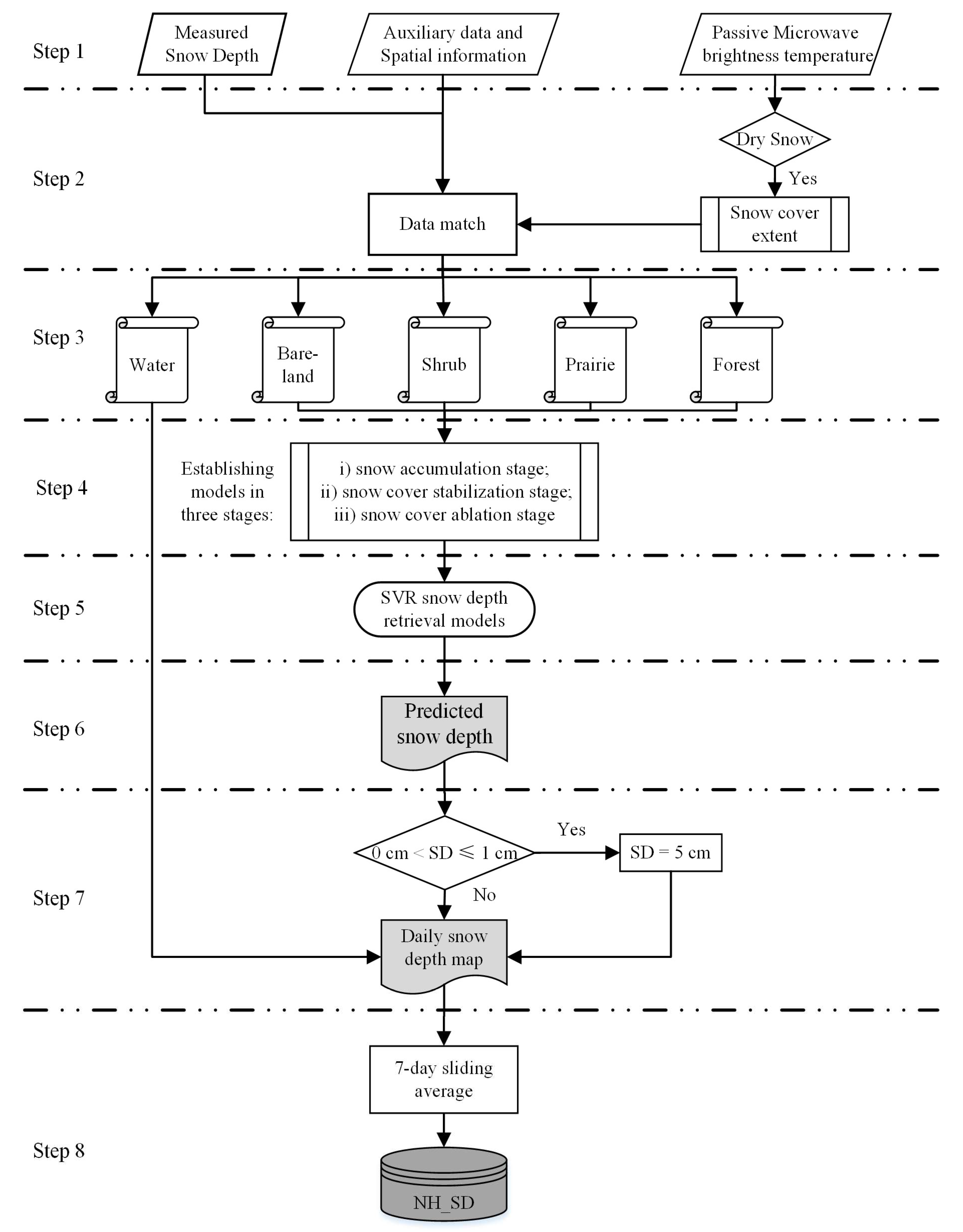
A previous study of the machine learning SVR method for SD retrieval models performed well with reduced uncertainties compared to the measured data from ground stations across the Eurasia region, based on analyzing the correlation coefficient (R), mean absolute error (MAE), and root mean squared error (RMSE) [24]. Here, we intended to use daily observational datasets over the Northern Hemisphere by applying the SVR method (except for July and August). The SVR SD retrieval algorithm uses a non-linear regression (support vector regression, SVR) method as the retrieval function (g (·) in Equation (1)). This machine learning (SVR) method was applied to establish the complex relationship between the target variable and input variables. Following Equation (1), we used ten variables as the inputs, including PM brightness temperature (19 GHz, 37 GHz, and 85 or 91 GHz) with vertical and horizontal polarizations, geographical location (latitude and longitude), elevation, and the measured SD. This algorithm also indirectly considered seasonal variation (day of the year; D) and vegetation (land cover; L) influence factors to improve the accuracy of the estimated SD. The output parameter is the estimated SD. This SVR SD retrieval algorithm mainly involves five steps (Steps 1–5). Steps 6–8 are the SD dataset generation processes (Figure 2).

Step 1. Involves pre-processing meteorological station SD measurements, PM brightness temperature data, and other auxiliary datasets (DEM, land cover, and spatiotemporal information). Before estimating the SD from the PM data, it is necessary to identify snow cover and dry snow by a set of criteria [75]; in the training stage, it should extract and match the station measurements, PM brightness temperature data (classified as snow cover), and other auxiliary information; and in the predicting stage, the PM brightness temperature and auxiliary information were preprocessed to the datasets (Step 2).

Step 3. we developed SD retrieval models based on four land cover types to segregate the land cover effects. For the years over which our study period pre-dated the MODIS data, we used AVHRR land cover as the supplement data. We reclassified MODIS and AVHRR land cover into four classes (forest, shrub, prairie, and bare-land), which were the bases for constructing the SD retrieval sub-model. Table A1 (in the Appendix A) describes the reclassification scheme for AVHRR land cover. The MODIS land cover reclassification schemes were documented in Xiao et al. [24]. Because of the relatively stable change in land cover, the MODIS land cover in 2013 was used for each year from 2013 to 2016. Similarly, the MODIS land cover in 2001 was used for each year from 1998 to 2001, and the AVHRR land cover data was used for each year from 1992 to 1997. The retrieval sub-models were established on different land cover types (forest, shrub, prairie, and bare-land).

Step 4. we converted the day of the year (D) effects into the following three snow cover stages: snow accumulation stage (September to November), stabilization stage (December to February), and ablation stage (March to June). To consider the evolution effect of the snow properties, the SD retrieval model was established based on these three snow cover stages.

Step 5. we chose SVR as the retrieval function (Equation (1)), with specific kernel functions and parameters [24]; the optimization of parameters for the selected method were performed in the training stage to improve the model performance in this study.

Step 5.1. construction of a sub-continental model. In this study, we separately constructed the SD retrieval models for Eurasia and North America, based on the information that the snow properties show a discrepancy between Eurasia and North America. Taking snow density as an example, Bilello [76] pointed out that the mean snow density in the former Soviet Union (0.21 ~ 0.31 g/cm³) was lower than that in North America (0.24 ~ 0.31 g/cm³). Zhong et al. [77] explained the reasons for such a difference between Eurasia and North America.

Step 5.2. selection of training sample. The accuracy of the estimated SD primarily depended on the quality of the training samples [24]. More data than needed in the training stage to train the SD retrieval model may lead to over-fitting and yield an estimated SD with a high error. In this study, we collected numerous daily records for over 25 years. A changed sample selection rule was used in this study to avoid data information redundancy, and was divided into two steps. First, the number of samples of the three groups split by snow depth values were solidly quantified, i.e., group 1 (0 cm ≤ SD < 50 cm; shallow snow), group 2 (50 cm ≤ SD < 100 cm; intermediate depth), and group 3 (SD ≥ 100 cm; deep snow). To avoid an inflated training sample in group 2 and group 3, we set a threshold value number of used datasets (3000) determined by several tests (not shown). The threshold of the number of samples (12,000) for group 1 was adopted.

Table 2. Training sample filter rules.

Group ID	Filter Rules
Group 2	If ${\mathrm{Number}}_{total}\left(group2\right)\le 3000$       ${\mathrm{Number}}_{training}\left(group2\right)=\left({\mathrm{Number}}_{total}\left(group2\right)\right)/2$ Else ${\mathrm{Number}}_{training}\left(group2\right)=3000$
Group 3	If ${\mathrm{Number}}_{total}\left(group3\right)\le 3000$       ${\mathrm{Number}}_{training}\left(group3\right)=\left({\mathrm{Number}}_{total}\left(group3\right)\right)/2$ Else ${\mathrm{Number}}_{training}\left(group3\right)=3000$
Group 1	If ${\mathrm{Number}}_{training}\left(group2\right)>2000$ or ${\mathrm{Number}}_{training}\left(group3\right)>1000$ ${\mathrm{Number}}_{training}\left(group1\right)=\mathrm{15,000}-{\mathrm{Number}}_{training}\left(group2\right)-{\mathrm{Number}}_{training}\left(group3\right)$ Else ${\mathrm{Number}}_{training}\left(group1\right)=\mathrm{12,000}$

details the selection rules for the training sample for each group. Second, the quality of the training sample in each group was controlled using stratified random sampling. Stratification was performed at 1-cm SD intervals, and in each interval value of the datasets, we operated random selection to choose the needed numbers of samples.

Step 6. Through the above steps, we generally created 24 SD retrieval sub-models (two (continents) * four (land classes) * and three (stages)), and then the preprocessed PM brightness temperature datasets were used to predict daily SD across the Northern Hemisphere from January 1992 to December 2016 (excluding July and August).

Step 7. The generated raw daily SD data were then processed to the daily SD map. If one pixel was detected as snow cover by the detection decision tree [75], but was likely to be shallow snow with an estimated value of equal or less than 1 cm in the raw predicted SD data, then the SD value was set as 5 cm [33,78] (Figure 2). Owing to the radiometer observations, the generated SD data were only reliable in areas with seasonal dry snow cover. Areas with sporadic wet or thin snow were not reliably detected, and areas marked as snow-free may have included areas with wet snow.

Step 8. This study excluded the Greenland and Iceland regions from the generation and analysis of the NHSnow datasets (NH_SD), because of the difficulty in discriminating snow from ice (Figure 2) [19]. Missing data and zero-data gaps occurred when generating the daily SD grid. We applied the following filter: the daily estimated SD was defined as the midpoint of a sliding seven-day average window in order to reduce noise and compensate for missing data in the daily time series. For example, the SD estimated for 4 January was an average of the assimilated scheme output for 1 to 7 January [17,33]. When finished, the sliding SD method generated full coverage daily SD datasets for the entire Northern Hemisphere (Figure 2).

3.3. Analysis Index Description

We used the seasonal maximum SD, seasonal average SD, and annual average SD as the SD analysis indexes to characterize the SD variability across the Northern Hemisphere. The seasonal maximum SD of a pixel refers to the maximum SD for a season (autumn: September–November; winter: December–February; spring: March–May). The sasonal average SD is defined as the cumulative SD divided by the days in one season (Equation (2)). The calculation of the annual average SD is similar to the seasonal average SD (Equation (2)).

$${\mathrm{SD}}_{average}=\frac{{{\displaystyle \sum }}_{i=1}^{n}S{D}_i}{n}$$

(2)

where $n$ is the number of days of one specific period, such as, a snow cover year (September–June) or a season (autumn, winter, or spring), and $i$ is $i$th day of this specific period. SD is snow depth.

The snow cover detection of the NHSnow SD data was based on Grody’s snow cover identification method [75]. This means that SD was derived when the ground was detected as snow cover. Therefore, snow cover days (SCDs) were defined as the number of days that the SD was over 0 cm in a snow cover year (from September 1 to June 30). When analyzing the SD and SCD variation from 1992 to 2016, we divided the variation trends into five grades (highly significant decrease, significant decrease, non-significant change, significant increase, and highly significant increase;

Table 3. Rules of variation trend grading.

Variation Rate	P Value	Variation Level
Rate < 0	P ≤ 0.01	Highly significant decrease
Rate < 0	0.01 < P ≤ 0.05	Significant decrease
-	P > 0.05	Non-significant change
Rate > 0	0.01 < P ≤ 0.05	Significant increase
Rate > 0	P ≤ 0.01	Highly significant increase

), and the significance of the trends was based on a t-test.

4. Results

4.1. Validation of Snow Depth Dataset

To provide insight into the relative performance of the SD datasets, we compared three sources of snow cover datasets (NHSnow, GlobSnow, and ERA-Interim/Land) with ground SD measurements (Figure 3, Figure 4, Figure 5, Figure 6, Figure 7 and Figure 8), using three indices (bias, mean absolute error (MAE), and root mean squire error (RMSE)). We collected daily SD measurements for the common period (1992–2010) of the three datasets as the validation data. This primarily focused on the snow stabilization stage (December to February). As the snow density changes slowly over a smaller range in the snow cover stabilization stage, we used a constant value (0.24 g/cm³) for GlobSnow. Note that the data used for validation in this section are completely independent of the dataset used for the SD retrieval models.

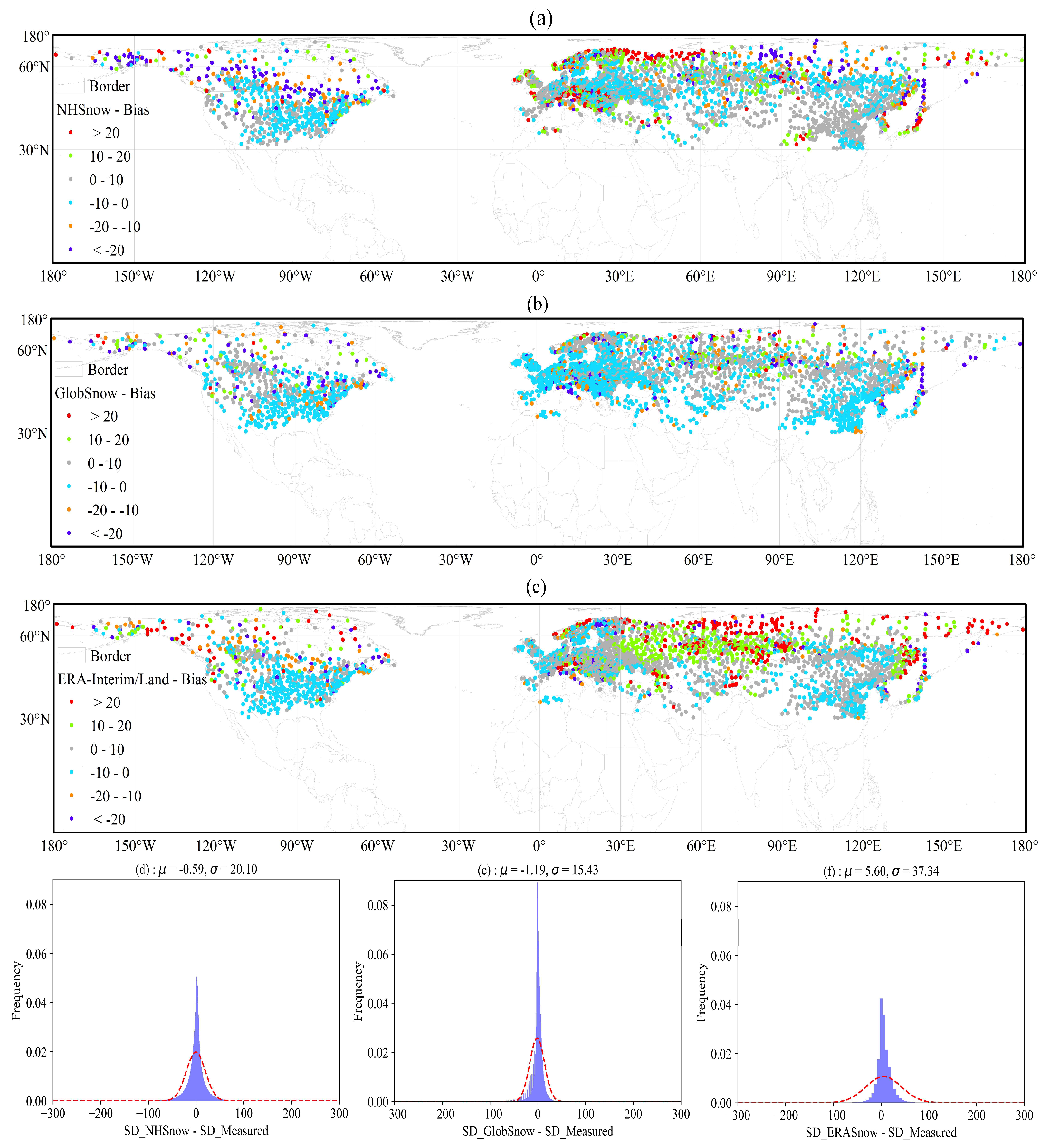
A small bias (blue and green dots in Figure 3) between the estimated SD against the measured SD was found for the mid and low latitude regions (<60° N) for the three SD datasets. However, a large bias was found for the Arctic region and along the coast, such as the Russian coastal regions, the Russian Far East, the Korean peninsula region, and Northeast Canada. For NHSnow and GlobSnow, bias was mostly distributed near the mean value μ = 0 line with a high frequency, although some bias was greater than 100 cm (or less than −100 cm; Figure 3d,e). Positive (negative) biases indicate that the mean estimated values are greater (less) than the corresponding measured SD values. ERA-Interim/Land overestimated the snow depth in Western Siberian Plains and Eastern European Plains (around 60° N; red dots, Figure 3c).

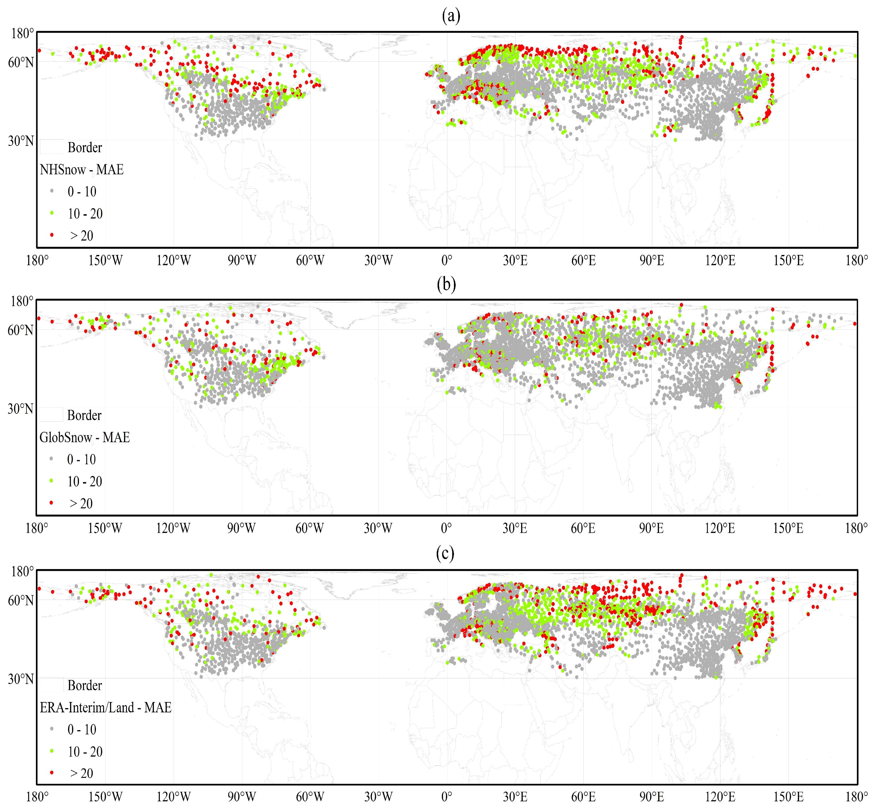
For the analysis indexes, MAE, and RMSE, the distribution of error points of NHSnow and GlobSnow were almost the same as the distribution of its bias (Figure 3, Figure 4 and Figure 5). We used all of the valid daily records for each evaluation station to calculate three precision indexes for the three snow cover datasets, and found that the bias, MAE, and RMSE were −0.59 cm, 15.98 cm, and 20.11 cm, respectively, for the NHSnow grid datasets. For GlobSnow, however, there was more bias (−1.19 cm), and a lower MAE (15.12 cm) and RMSE (15.48 cm;

Table 4. The evaluated bias, MAE, and RMSE (unit cm) for three grid SD datasets (NHSnow, GlobSnow, and ERA-Interim/Land).

Datasets	Bias	MAE	RMSE
NHSnow	−0.59	15.98	20.11
GlobSnow	−1.19	15.12	15.48
ERA-Interim/Land	5.60	18.72	37.77

). This comparison (NHSnow vs. GlobSnow) showed a relatively good agreement, although NHSnow over- or under-estimated the SD with a larger RMSE. Overall, the performance of GlobSnow was better than the NHSnow grid data. However, part of the validation data was also applied for the GlobSnow assimilation; it is highly possible that, in this case, the GlobSnow validation may not have been completely independent. The grain size was more important than the snow density and temperature in the microwave emission modeling. The different performances for these two datasets might have been mainly caused by the variation of the snow grain size, which was used to generate the SWE of GlobSnow [17]. Che et al. [33] reported that the grain size is more important than snow density and temperature. Furthermore, ERA-Interim/Land had the worst performance of all of the three snow cover datasets, with the highest bias (5.60 cm), MAE (18.72 cm), and RMSE (37.77 cm). The smallest bias was found for the mid-latitude regions (<50° N), and much of the bias lay at 0–100 cm for ERA-Interim/Land (Figure 3c,f). We found large MAE and RMSE in the high latitude and coastal regions (Figure 3c). Unlike NHSnow and GlobSnow, ERA-Interim/Land was more likely to overestimate SD, and appeared to be less consistent with the in situ observations across the Northern Hemisphere (Figure 3f).

4.2. Variation of Snow Depth

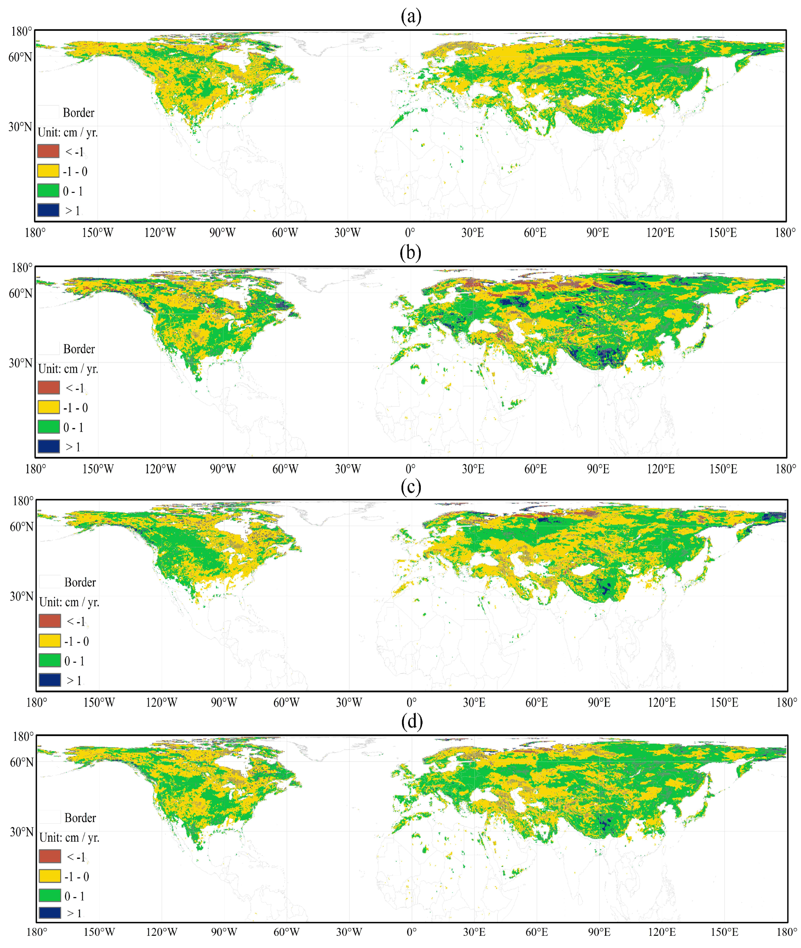
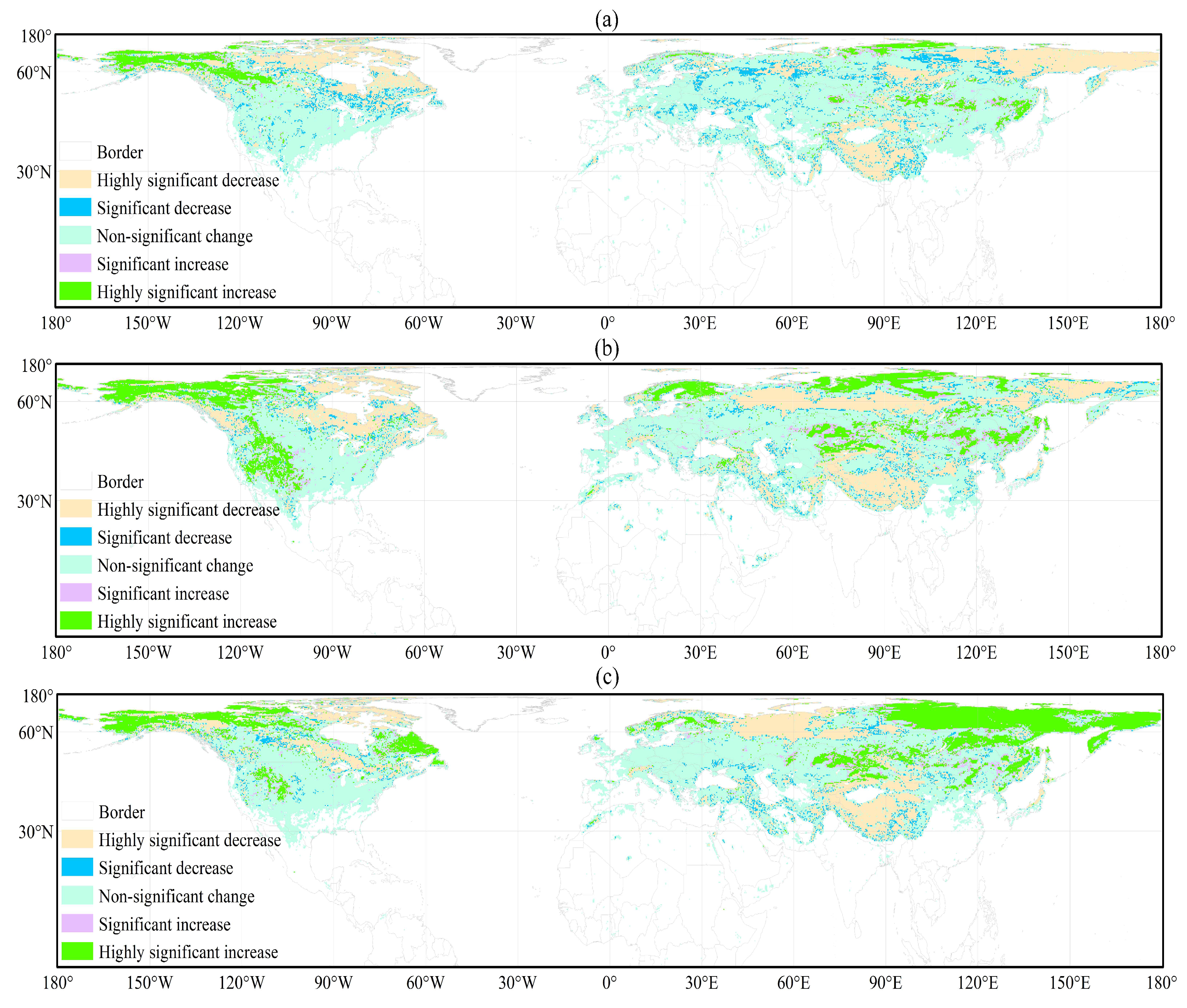
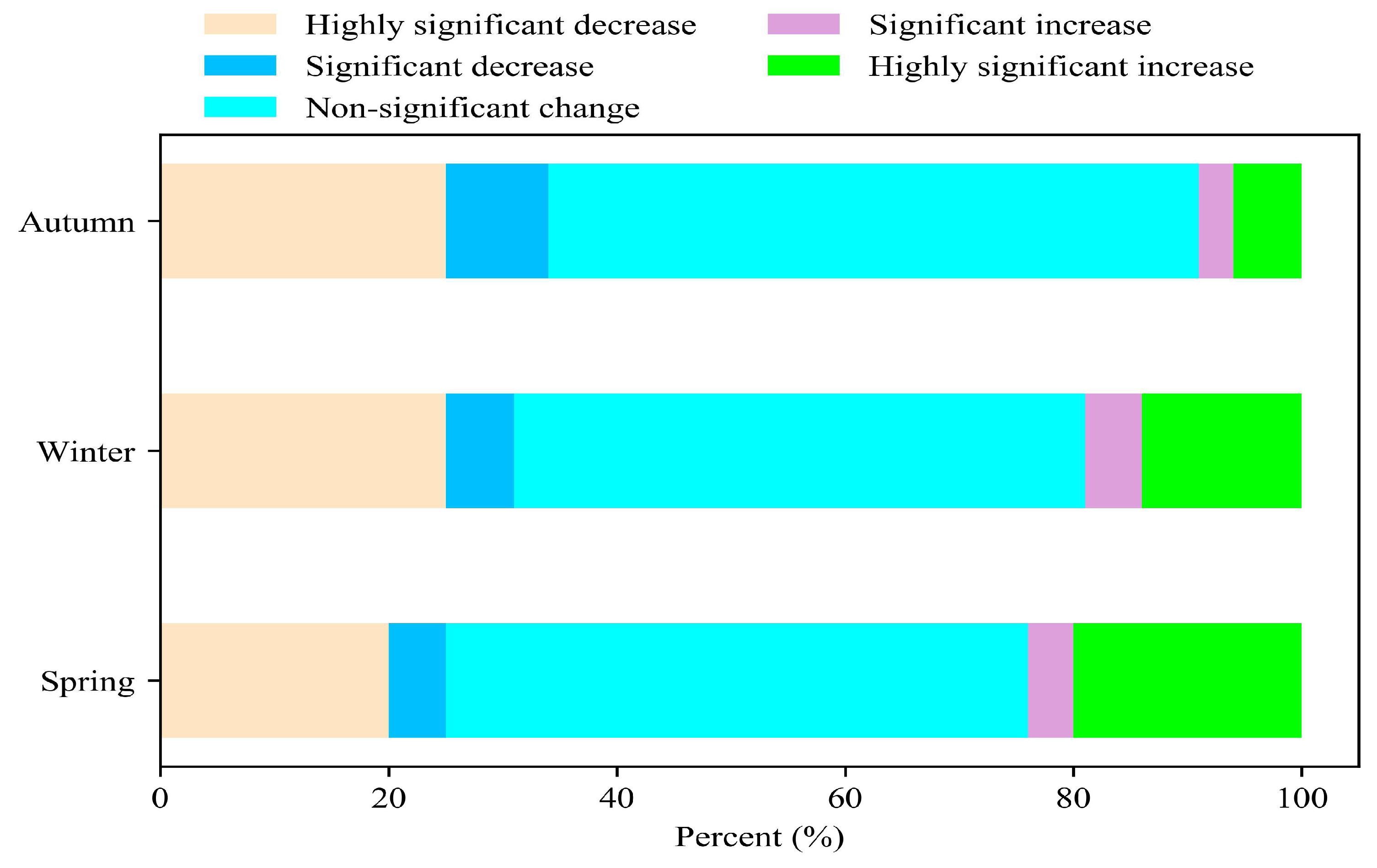
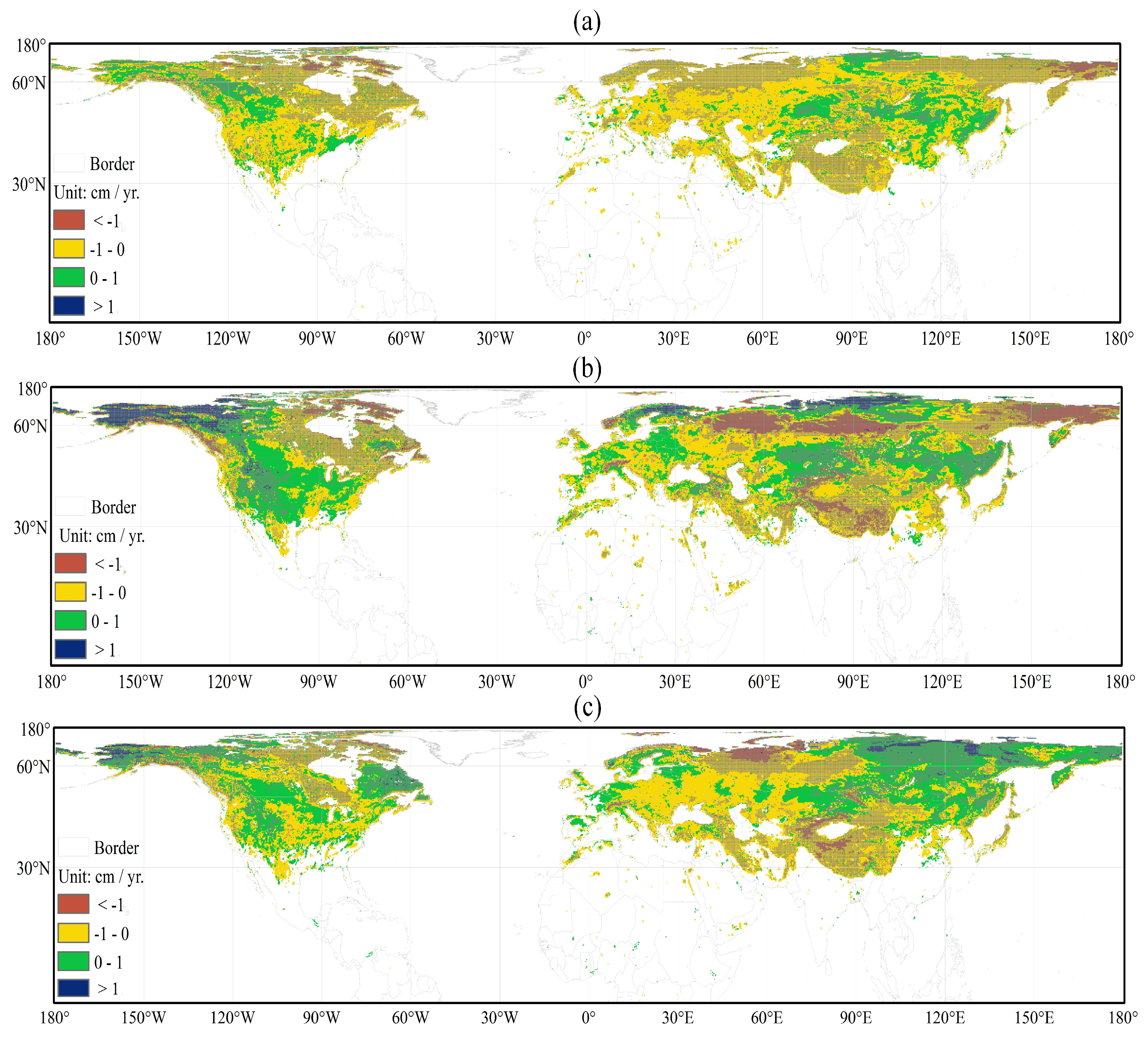
To understand and interpret snow cover variations better in the Northern Hemisphere, we analyzed the SD variation using the seasonal maximum SD of the NHSnow dataset from 1992 to 2016 with variation trend grading (Table 3; Figure 6). The variation trend of the seasonal maximum SD exhibited distinctly different patterns in the three seasons during 1992–2016. Spatially, we found that the areas where SD exhibited a highly significant decrease trend in autumn (Figure 6a) were mainly located in the Russian Far East, the Qinghai–Tibet Plateau, the south of the central Siberian Plateau, and the northeastern regions of Canada. Over Russia’s Taimyr Peninsula and the Alaska region, SD exhibited a highly significant increase trend (0–1 cm yr⁻¹). Moreover, the seasonal maximum SD in winter and spring also underwent a highly significant decrease trend in the Qinghai–Tibet Plateau and the northeastern region of Canada (Figure 6b,c). The areas with a highly significant SD decrease extended to the Western Siberian plain region. Wang and Li [79] used nearly 50 years of daily station SD observation data to analyze the trend of maximum SD in China, and found that variation trend of the seasonal maximum SD in the Qinghai–Tibet Plateau was consistent with the observations from this study. The seasonal maximum SD variations in autumn and winter in the Russian Far East area exhibited a highly significant decreasing trend, while in spring, it showed a highly significant increasing trend. This variation trend pattern of the NHSnow seasonal maximum SD in spring was consistent with the analysis results obtained using the GlobSnow datasets [80], showing increasing trends in the Scandinavian peninsula and Alaska regions, and decreasing trends in the Kamchatka Peninsula region. We quantified the proportion of each of the variation trend grades in each season, because the snow cover area varied between seasons. From Figure 7, non-significant change dominated the seasonal maximum SD variation trends of the Northern Hemisphere (more than 50%) in three seasons. There were more regions (green regions) with a (highly) significant decrease trend of seasonal maximum SD in winter and spring, accounting for 31% and 34%, respectively, while the areas showing (highly) significant increasing trends (19% and 8%) were less. As for spring, the proportion of area with an increasing trend (about 25%) in the seasonal maximum SD was slightly larger than the decreasing trend (about 24%).

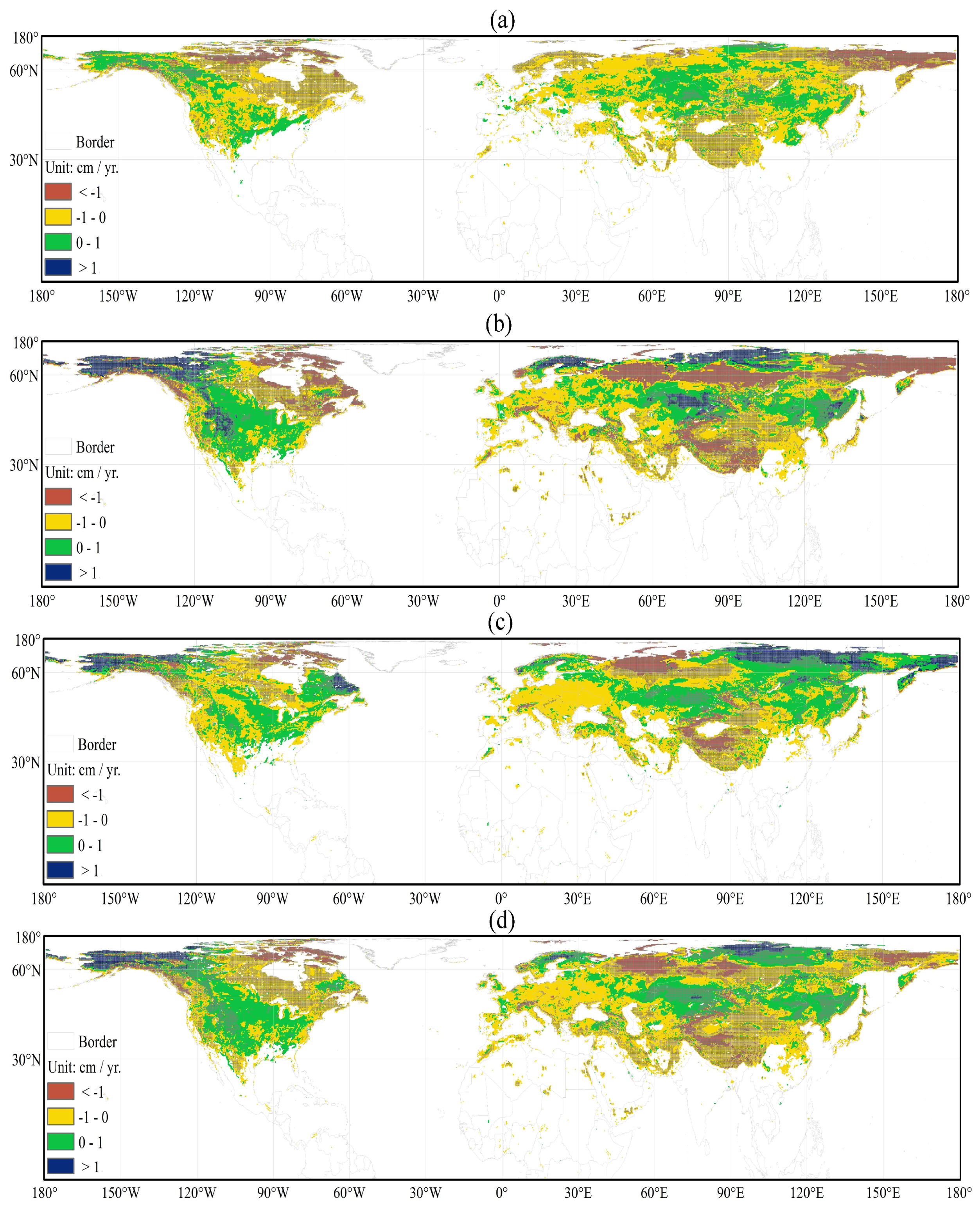
Finally, we analyzed the variation pattern of the average SD across the Northern Hemisphere using the average SD for each season. The variation rate of each season’s average SD exhibited great fluctuations in different regions and seasons. The winter average SD decreased with the highest rate of −0.11 cm yr⁻¹ compared with the other two seasons during 1992–2016 (Figure 8b;

Table 5. Mean variation rate of the average SD (cm yr⁻¹) over the Northern Hemisphere for the three study periods (1992–2016, 1992–2001, and 2002–2016) and snow cover seasons (autumn, winter, and spring). Std. is standard deviation.

Season	1992–2016 (Mean ± 1 Std.)	1992–2001 (Mean ± 1 Std.)	2002–2016 (Mean ± 1 Std.)
Autumn	−0.08 ± 0.11	−0.01 ± 0.19	−0.15 ± 0.22
Winter	−0.11 ± 0.40	0.06 ± 0.62	−0.22 ± 0.75
Spring	−0.04 ± 0.25	0.02 ± 0.51	−0.07 ± 0.41
Year	−0.06 ± 0.20	0.02 ± 0.35	−0.11 ± 0.34

). In particular, the seasonal average SD variation rate in the Arctic region fluctuates greatly from region to region far more than average (Figure 8 and Figure 9). Additionally, the absolute values of the seasonal average SD variation rate in the Arctic regions were apparently larger than in the middle–low latitude regions (Figure 8 and Figure 9; Figure A1 and Figure A2 in Appendix A). These results are indeed consistent with station observations over Northern Russia [81], Northern Canada [82], and Alaska. The average seasonal SD in the Northern Hemisphere is subject to a large standard deviation. A similar conclusion can be found in the two periods of 1992–2001 and 2002–2016 (Figure A1 and Figure A2 in Appendix A; Table 5). The majority regions in the Northern Hemisphere showed increasing trends in seasonal average SD during 1992–2001 at the rate of 0.02 cm yr⁻¹ (Figure A1 and Table 5). However, the seasonal average SD variation trend during 2002–2016 was reversed, presenting decreasing trends (autumn: 0.15 cm yr⁻¹; winter: 0.22 cm yr⁻¹; and spring 0.07 cm yr⁻¹). The absolute variation rate during 2002–2016 was apparently greater than the rate during 1992–2001 (Figure A2 and Table 5). We found that a high absolute value of the SD variation rate (>1 cm yr⁻¹) usually occurred in the Arctic and the Qinghai–Tibetan plateau for all three seasons. The snowpack inevitably contained liquid water, as snow melting events occurred especially in spring. During the spring periods, consequently, the SD and snow cover days derived from the NHSnow datasets were partly underestimated and bias might have occurred in the trend change analysis of snow cover. The breakpoint time (2001/2002) was selected because it was the beginning of the new century.

4.3. Snow Cover Days

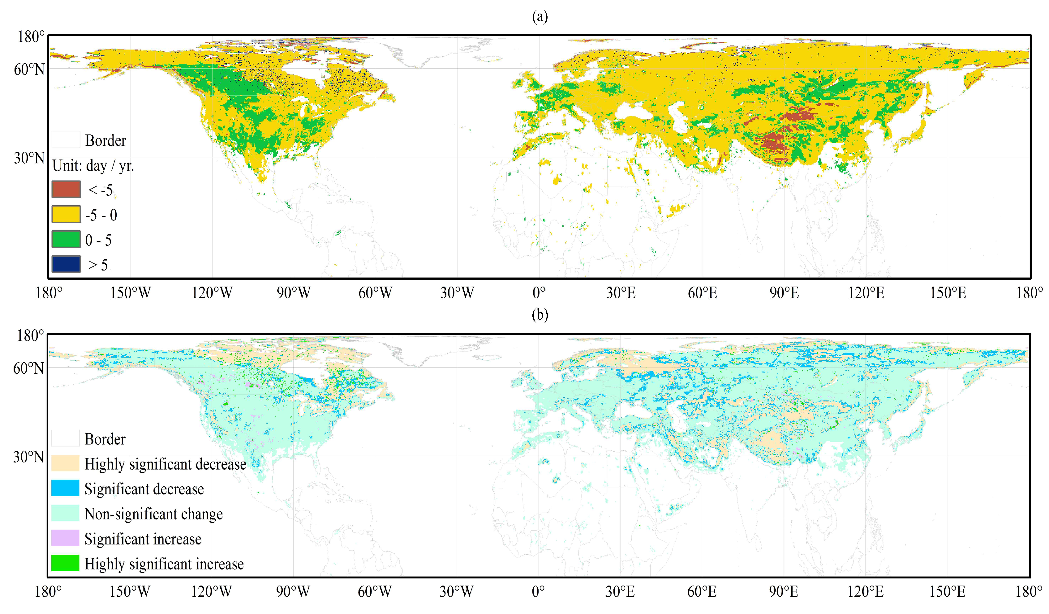
Investigating the variation of SCD showed a rate of −0.99 ± 2.23 day yr⁻¹ during 1992–2016. Most areas across the Northern Hemisphere presented a prominent decreasing trend, with the decreasing rate ranging from 0 to 5 day yr⁻¹ (Figure 10a). The decreasing trend regions are mainly distributed in Eurasia, covering a vast area of the northern Russia and central Asia. The regions with a decreasing rate greater than 5 day yr⁻¹ were almost all located in China, for example the Qilian Mountain, central Tibetan Plateau, and Tianshan regions. The regions with increasing trends were found in the central North America, Western Europe, Northwestern Mongolia, and some areas of China. Throughout the Northern Hemisphere (Figure 10a), the areas with decreasing trends covered the most regions, spanning from 25° N through 85° N, with a mean decreasing rate of approximately 1 day yr⁻¹. The most notable variation (either decrease or increase) occurred in the Arctic regions (Figure 10b).

Unlike the SCD variation rate pattern, the SCD variation trend showed that the majority of regions (approximately 64%) demonstrated a non-significant change over the Northern Hemisphere (Figure 10b; Figure A3 in the Appendix A). The highly significant decrease and the significant decrease trend, which appeared in the northwest of Hudson Bay in Canada, the Kamchatka peninsula, the Eastern European plains, Northern Russia, the Iranian plateau, and several regions in China (the Tibet Plateau, Mount Tianshan, and Northeast China Plain), accounted for 33% of the total snow cover area. In addition, areas with a highly significant decrease and significant increase trend (3%) were only found in a limited area of North America and the eastern Qinghai–Tibetan Plateau regions.

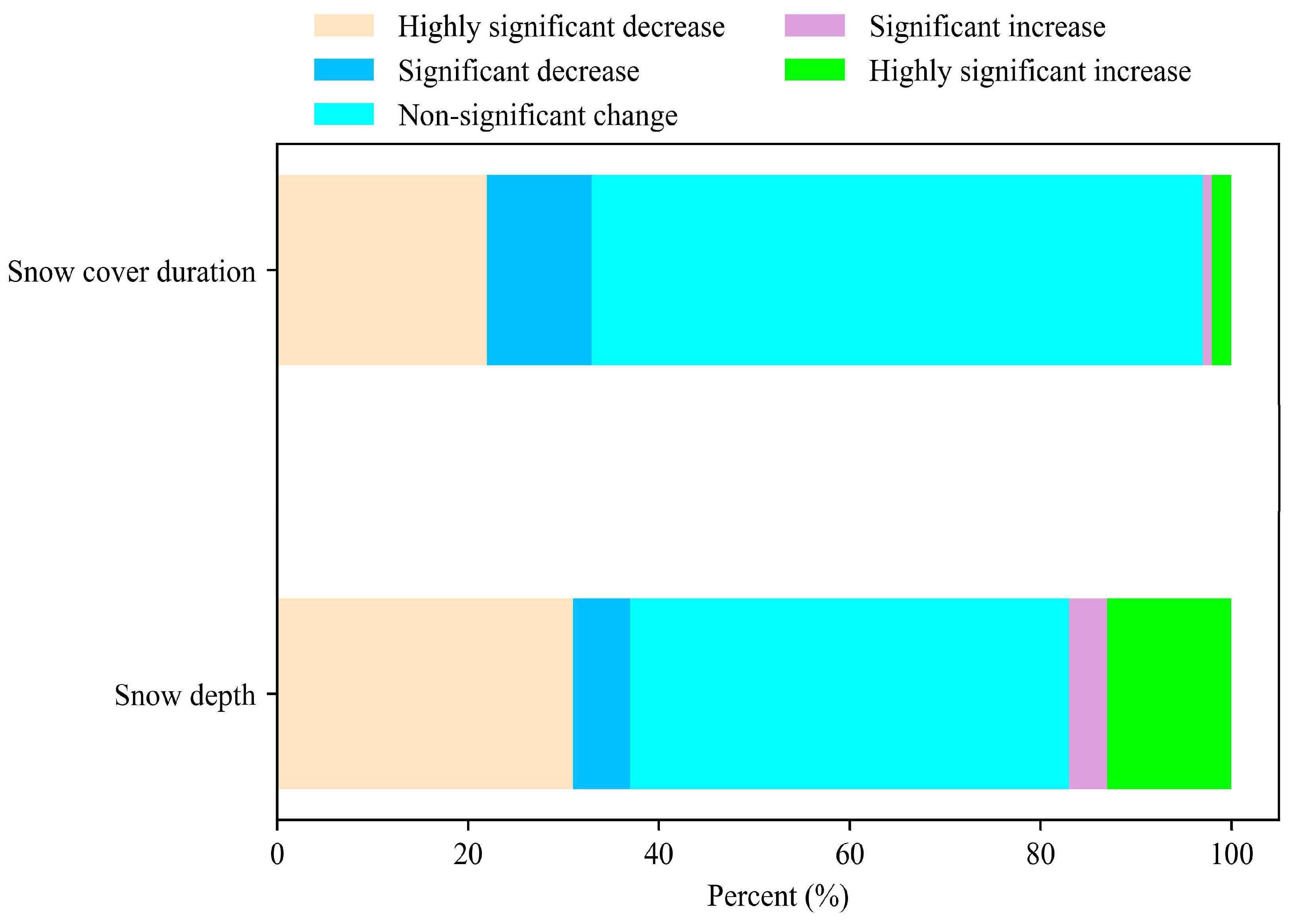
In terms of the changes in SCD and the annual average SD, they were either in the same or opposite directions over the past few decades. We found that the area where the annual average SD changed significantly (increase or decrease) was apparently larger than that of SCD (54% vs. 36%; Figure A3 in the Appendix A). Generally, more than 60% of a snow cover area has the same variation trends for the SCD and annual average SD (Figure 11), and the remaining area (40%) had different variation trends (non-significant change or a significant increase or decrease). Interestingly, the areas with the opposite trend of variation in SCD and annual average SD were approximately 20%, i.e., areas with a significant increasing trend in the annual average SD while showing the SCD with a significant decreasing trend in the corresponding areas (pink area in Figure 11; 4%), and areas with a significant decreasing trend of annual average SD, while showing the SCD with a significant increasing trend (blue area in Figure 11; 16%). These regions with the opposite trend (increasing for annual average SD but decreasing for SCD) mostly appeared in the northern Central Siberian Plateau, the eastern Scandinavian Peninsula, Western Alaska, and the northern Greater Khingan Mountains of China. Zhong et al. [83] reported similar results across the northern Eurasian continent using ground-based measurements. As a reference, we also analyzed the variation trends of SCD and annual maximum SD (Figure A4 in the Appendix A), showing that the areas with the opposite trend of variation in SCD and the annual maximum SD accounted for 21%. The pattern of these variation trend areas was also the same as the pattern for the SCD and annual average SD, except for a few areas (Figure 11 vs. Figure A4). The increase in SD may be explained by the increasing frequency of extreme snowfall [83]. Additionally, a recent study found that the greater the SWE, the faster the melting rate, leading to a shortened SCD in the Northern Hemisphere [80], along with an increasing winter air temperature [81,82]. Furthermore, the areas showing an annual average SD significantly decreased, but SCD significantly increased, accounting for 16% of the total snow cover area, mainly distributed in regions around 60° N and the margin of the Qinghai–Tibetan Plateau.

5. Discussion

While these three gridded data (NHSnow, GlobSnow, and ERA-Interim/Land) do a fairly good job in small SD accumulations (shallow and mid-deep snow cover) regions, they all struggle to capture SDs with a low bias, MAE, and RMSE in high SD accumulation (deep snow) regions (Figure 3, Figure 4 and Figure 5). There are insurmountable saturation effects in deep snowpacks when using passive microwave remote sensing data [24,84]. All of the SD retrieval algorithms based on the attenuation of radiation have insensitivity to deep snow. As a result, the snow cover variation could not be adequately captured in areas with deep snow; thus, we should be cautious when interpreting the validation result in deep snow regions.

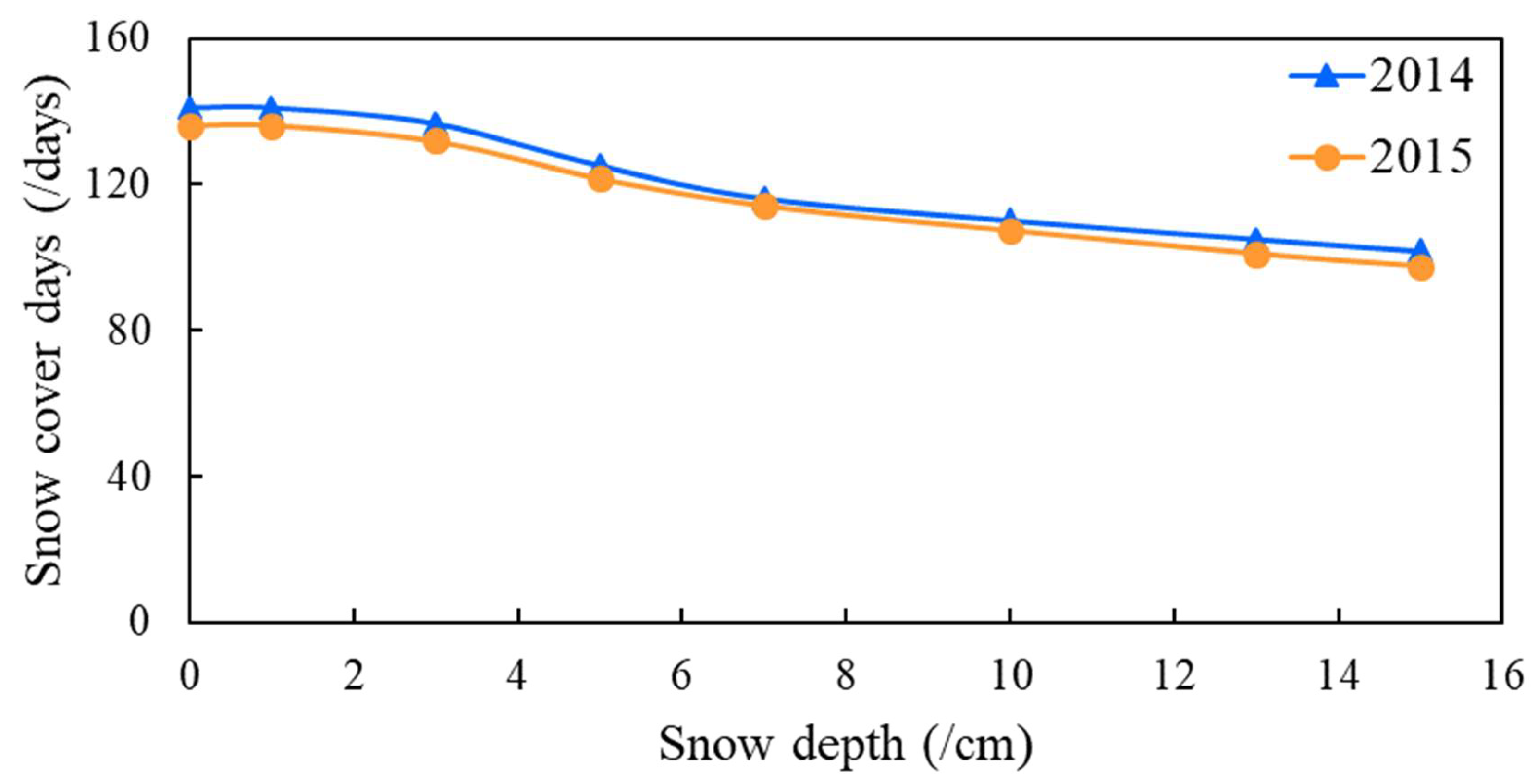
It should be noted that snow-covered area of NHSnow was dry snow, as determined by Grody’s series of rules [75]. SCD is determined on the identified snow-covered area [24,75]. The threshold of SD may have an effect on the specific value of the generated SCD. The sensitivity of SCD to the SD threshold changes were analyzed using two datasets (September 2014 to June 2015; September 2015 to June 2016; Figure 12). We found that the low threshold of SD (<3 cm) used to define the SCD did not significantly change the value of SCD, while a high value for SD could have significant decrease for SCD and snow cover extent, as reported by [49]. When compared to the SCD derived from optical sensor data, the specific quantity of SCD and the SCD variation rate derived from the NHSnow data was overestimated. As the optical (MODIS or AVHRR) and microwave sensors (SSM/I or AMSR-E) respond to different parts of the electromagnetic spectrum, the estimated snow cover area and SCD from these two sensors would vary somewhat [51,85]. Notwithstanding, another explanation for these discrepancies may be the snow cover identification algorithm [25,86,87]. The microwave radiation characteristics of snow cover are similar to that of precipitation, cold desert, and frozen ground [75]. Commission and omission errors in the NHSnow datasets may result from coarse spatial resolution, snow characteristics and topography [21], and precipitation [75,86], especially over frozen ground [88]. Several rules for NHSnow algorithm development were applied to distinguish snow from precipitation, cold desert, and frozen ground [24]; it was impossible to entirely remove interference factors in each image at the current studies. Moreover, the precondition of NHSnow is dry snow, which means almost no wet snow was considered in the SCD variation analysis [89]. The poorer performance of the microwave derived datasets was anticipated because of the documented difficulties in monitoring snow cover over forested and mountainous terrain [34,73].

6. Conclusions

This study applied the revised support vector regression snow-depth retrieval algorithm, which uses passive microwave remote sensing and other auxiliary data to generate long term (1 January 1992, to 31 December 2016) Northern Hemisphere daily snow depth (SD) datasets (NHSnow) with a 25-km spatial resolution. When compared to the other snow cover datasets (GlobSnow and ERA-Interim/Land) benchmarked against the ground SD measurements, the NHSnow SD datasets had a relatively smaller bias (−0.59 cm), mean absolute error (15.12 cm), and root mean square error (20.11 cm).

NHSnow datasets with full coverage and high accuracy can provide useful information about the spatiotemporal distribution of snow cover. We quantificationally investigated the spatial and temporal change characteristics in snow cover (SD and SCD) across the Northern Hemisphere. The analysis results show that the SD variation pattern in the variation rate or variation trend (increase or decrease) varies greatly among the different areas. For the seasonal maximum SD, areas with a significant decreasing trend are larger than those with a significant increasing trend in three seasons, namely, autumn (34% vs. 8%), winter (31% vs. 19%), and spring (25% vs. 24%). The results show that the annual average SD decreased at a rate of −0.06 cm yr⁻¹ from 1992 to 2016 across the Northern Hemisphere, and the variation rate in winter was the highest, reaching up to −0.11 cm yr⁻¹; meanwhile, the absolute values of the variation rate of the seasonal average SD in the most Arctic regions are apparently greater than that in the middle–low latitude regions. In terms of the spatiotemporal variation trend of SCD over the Northern Hemisphere, we found that most areas show non-significant variation trends (more than 64%), while 33% of the area shows a significant decreasing trend. Interestingly, we found that only 60% of areas show the same variation trends for the SCD and annual average SD, but the area presenting a completely opposite variation trend for the SCD and annual average SD accounts for 20% of the total snow cover area, occurring in part of the Arctic regions and in the third polar region (Tibetan Plateau).

While this study shed light on the spatiotemporal variability trends of snow cover across the Northern Hemisphere using the 25-year NHSnow datasets, we cannot claim that the NHSnow dataset could completely capture the climate change signal in each region and season. Compared to the current relative best snow cover datasets, there are some deficiencies and limitations (e.g., overestimation and underestimation) for the NHSnow datasets, and further efforts should be made to improve the estimation accuracy and robustness of the SD inversion algorithm coupling the snow physical model/radiative transfer model, which appears to be a promising approach [27,90,91]. Meanwhile, a comprehensive validation analysis should also be carried out in complex terrain regions and different land cover types [21,22,92]. Further analyses and study are still needed to help understand the characteristics of SD changes in the Northern Hemisphere, e.g., analyzing and investigating the difference of snow cover variation and its response to climate change in regional and continental areas [17,93,94,95]. It is recommended that future works focus on the climatic effects and climatological causes in snow cover changes in order to comprehensively understand the associated snow cover change mechanisms against a climate change background [5,7,50,66].

References

1. Immerzeel, W.W.; Van Beek, L.P.H.; Bierkens, M.F.P. Climate change will affect the Asian Water Towers. Science 2010, 328, 1382–1385. [Google Scholar] [CrossRef] [PubMed]
2. Zhang, T. Influence of the seasonal snow cover on the ground thermal regime: An overview. Rev. Geophys. 2005, 43, 589–590. [Google Scholar] [CrossRef]
3. Robinson, D.; Frei, A. Seasonal Variability of Northern Hemisphere Snow Extent Using Visible Satellite Data. Prof. Geogr. 2000, 52, 307–315. [Google Scholar] [CrossRef]
4. Tedesco, M.; Derksen, C.; Deems, J.; Foster, J.L. Remote sensing of snow depth and snow water equivalent. Remote Sens. Cryosphere 2014, 73–98. [Google Scholar] [CrossRef]
5. Flanner, M.G.; Shell, K.M.; Barlage, M.; Perovich, D.K.; Tschudi, M.A. Radiative forcing and albedo feedback from the Northern Hemisphere cryosphere between 1979 and 2008. Nat. Geosci. 2011, 4, 151–155. [Google Scholar] [CrossRef]
6. Zhang, T.; Osterkamp, T.E.; Stamnes, K. Influence of the Depth Hoar Layer of the Seasonal Snow Cover on the Ground Thermal Regime. Water Resour. Res. 1996, 32, 2075–2086. [Google Scholar] [CrossRef]
7. Cohen, J.; Furtado, J.C.; A Barlow, M.; Alexeev, V.A.; E Cherry, J. Arctic warming, increasing snow cover and widespread boreal winter cooling. Environ. Res. Lett. 2012, 7, 014007. [Google Scholar] [CrossRef]
8. Li, W.; Guo, W.D.; Qiu, B.; Xue, Y.; Hsu, P.-C.; Wei, J. Influence of Tibetan Plateau snow cover on East Asian atmospheric circulation at medium-range time scales. Nat. Commun. 2018, 9, 4243. [Google Scholar] [CrossRef] [Green Version]
9. Diffenbaugh, N.S.; Scherer, M.; Ashfaq, M. Response of snow-dependent hydrologic extremes to continued global warming. Nat. Clim. Chang. 2012, 3, 379–384. [Google Scholar] [CrossRef] [Green Version]
10. Barnett, T.P.; Adam, J.C.; Lettenmaier, D.P. Potential impacts of a warming climate on water availability in snow-dominated regions. Nature 2005, 438, 303–309. [Google Scholar] [CrossRef]
11. Sturm, M. White water: Fifty years of snow research in WRR and the outlook for the future. Water Resour. Res. 2015, 51, 4948–4965. [Google Scholar] [CrossRef]
12. Qin, D.; Liu, S.; Li, P. Snow cover distribution, variability, and response to climate change in western China. J. Clim. 2006, 19, 1820–1833. [Google Scholar]
13. Brown, R.; Frei, A. Comment on “Evaluation of surface albedo and snow cover in AR4 coupled models” by A. Roesch. J. Geophys. Res. Space Atmos. 2007, 112. [Google Scholar] [CrossRef]
14. Foster, J.; Hall, D.K.; Eylander, J.B.; Riggs, G.A.; Nghiem, S.V.; Tedesco, M.; Kim, E.; Montesano, P.M.; Kelly, R.E.J.; Casey, K.A.; et al. A blended global snow product using visible, passive microwave and scatterometer satellite data. Int. J. Remote. Sens. 2011, 32, 1371–1395. [Google Scholar] [CrossRef]
15. Chang, A.; Foster, J.; Hall, D. Nimbus-7 SMMR derived global snow cover parameters. Ann. Glaciol. 1987, 9, 39–44. [Google Scholar] [CrossRef] [Green Version]
16. Che, T.; Li, X.; Jin, R.; Armstrong, R.; Zhang, T. Snow depth derived from passive microwave remote-sensing data in China. Ann. Glaciol. 2008, 49, 145–154. [Google Scholar] [CrossRef] [Green Version]
17. Takala, M.; Luojus, K.; Pulliainen, J.; Derksen, C.; Lemmetyinen, J.; Kärnä, J.-P.; Koskinen, J.; Bojkov, B. Estimating northern hemisphere snow water equivalent for climate research through assimilation of space-borne radiometer data and ground-based measurements. Remote Sens. Environ. 2011, 115, 3517–3529. [Google Scholar] [CrossRef]
18. Pulliainen, J.; Luojus, K.; Derksen, C.; Mudryk, L.; Lemmetyinen, J.; Salminen, M.; Ikonen, J.; Takala, M.; Cohen, J.; Smolander, T.; et al. Patterns and trends of Northern Hemisphere snow mass from 1980 to 2018. Nature 2020, 581, 294–298. [Google Scholar] [CrossRef]
19. Brown, R.; Derksen, C.; Wang, L. A multi-data set analysis of variability and change in Arctic spring snow cover extent, 1967–2008. J. Geophys. Res. Space Phys. 2010, 115. [Google Scholar] [CrossRef]
20. Brown, R.; Robinson, D. Northern Hemisphere spring snow cover variability and change over 1922–2010 including an assessment of uncertainty. Cryosphere 2011, 5, 219–229. [Google Scholar] [CrossRef] [Green Version]
21. Dai, L.; Che, T.; Ding, Y.; Hao, X. Evaluation of snow cover and snow depth on the Qinghai–Tibetan Plateau derived from passive microwave remote sensing. Cryosphere 2017, 11, 1933–1948. [Google Scholar] [CrossRef] [Green Version]
22. Snauffer, A.; Hsieh, W.W.; Cannon, A. Comparison of gridded snow water equivalent products with in situ measurements in British Columbia, Canada. J. Hydrol. 2016, 541, 714–726. [Google Scholar] [CrossRef]
23. Dai, L.; Che, T.; Wang, J.; Zhang, P. Snow depth and snow water equivalent estimation from AMSR-E data based on a priori snow characteristics in Xinjiang, China. Remote. Sens. Environ. 2012, 127, 14–29. [Google Scholar] [CrossRef]
24. Xiao, X.; Zhang, T.; Zhong, X.; Shao, W.; Li, X. Support vector regression snow-depth retrieval algorithm using passive microwave remote sensing data. Remote. Sens. Environ. 2018, 210, 48–64. [Google Scholar] [CrossRef]
25. Foster, J.; Chang, A.; Hall, D. Comparison of snow mass estimates from a prototype passive microwave snow algorithm, a revised algorithm and a snow depth climatology. Remote. Sens. Environ. 1997, 62, 132–142. [Google Scholar] [CrossRef]
26. Kwon, Y.; Yang, Z.-L.; Zhao, L.; Hoar, T.J.; Toure, A.M.; Rodell, M. Estimating Snow Water Storage in North America Using CLM4, DART, and Snow Radiance Data Assimilation. J. Hydrometeorol. 2016, 17, 2853–2874. [Google Scholar] [CrossRef]
27. LaRue, F.; Royer, A.; De Sève, D.; Roy, A.; Cosme, E. Assimilation of passive microwave AMSR-2 satellite observations in a snowpack evolution model over northeastern Canada. Hydrol. Earth Syst. Sci. 2018, 22, 5711–5734. [Google Scholar] [CrossRef] [Green Version]
28. Charrois, L.; Cosme, E.; Dumont, M.; Lafaysse, M.; Morin, S.; Libois, Q.; Picard, G. On the assimilation of optical reflectances and snow depth observations into a detailed snowpack model. Cryosphere 2016, 10, 1021–1038. [Google Scholar] [CrossRef] [Green Version]
29. De Lannoy, G.J.M.; Reichle, R.; Arsenault, K.R.; Houser, P.R.; Kumar, S.; Verhoest, N.E.C.; Pauwels, V.R.N. Multiscale assimilation of Advanced Microwave Scanning Radiometer-EOS snow water equivalent and Moderate Resolution Imaging Spectroradiometer snow cover fraction observations in northern Colorado. Water Resour. Res. 2012, 48. [Google Scholar] [CrossRef]
30. Toure, A.M.; Reichle, R.H.; Forman, B.A.; Getirana, A.; De Lannoy, G. Assimilation of MODIS Snow Cover Fraction Observations into the NASA Catchment Land Surface Model. Remote. Sens. 2018, 10, 316. [Google Scholar] [CrossRef] [Green Version]
31. Saberi, N.; Kelly, R.; Flemming, M.; Li, Q. Review of snow water equivalent retrieval methods using spaceborne passive microwave radiometry. Int. J. Remote. Sens. 2019, 41, 996–1018. [Google Scholar] [CrossRef]
32. Gan, T.Y.; Barry, R.G.; Gizaw, M.; Gobena, A.; Balaji, R. Changes in North American snowpacks for 1979–2007 detected from the snow water equivalent data of SMMR and SSM/I passive microwave and related climatic factors. J. Geophys. Res. Atmos. 2013, 118, 7682–7697. [Google Scholar] [CrossRef]
33. Che, T.; Dai, L.; Zheng, X.; Li, X.; Zhao, K. Estimation of snow depth from passive microwave brightness temperature data in forest regions of northeast China. Remote. Sens. Environ. 2016, 183, 334–349. [Google Scholar] [CrossRef]
34. Jagt, B.V.; Durand, M.; Margulis, S.A.; Kim, E.J.; Molotch, N.P. The effect of spatial variability on the sensitivity of passive microwave measurements to snow water equivalent. Remote. Sens. Environ. 2013, 136, 163–179. [Google Scholar] [CrossRef]
35. Goïta, K.; Walker, A.E.; Goodison, B.E. Algorithm development for the estimation of snow water equivalent in the boreal forest using passive microwave data. Int. J. Remote. Sens. 2003, 24, 1097–1102. [Google Scholar] [CrossRef]
36. Derksen, C.; Walker, A.; Goodison, B. Evaluation of passive microwave snow water equivalent retrievals across the boreal forest/tundra transition of western Canada. Remote. Sens. Environ. 2005, 96, 315–327. [Google Scholar] [CrossRef]
37. Foster, J.L.; Hall, D.K.; Kelly, R.E.J.; Chiu, L. Seasonal snow extent and snow mass in South America using SMMR and SSM/I passive microwave data (1979–2006). Remote Sens. Environ. 2009, 113, 291–305. [Google Scholar] [CrossRef] [Green Version]
38. Durand, M.; Kim, E.J.; Margulis, S.A.; Molotch, N.P. A First-Order Characterization of Errors from Neglecting Stratigraphy in Forward and Inverse Passive Microwave Modeling of Snow. IEEE Geosci. Remote. Sens. Lett. 2011, 8, 730–734. [Google Scholar] [CrossRef]
39. Sandells, M.; Essery, R.L.; Rutter, N.; Wake, L.; Leppänen, L.; Lemmetyinen, J. Microstructure representation of snow in coupled snowpack and microwave emission models. Cryosphere 2017, 11, 229–246. [Google Scholar] [CrossRef] [Green Version]
40. Roy, A.; Royer, A.; St-Jean-Rondeau, O.; Montpetit, B.; Picard, G.; Mavrovic, A.; Marchand, N.; Langlois, A. Microwave snow emission modeling uncertainties in boreal and subarctic environments. Cryosphere 2016, 10, 623–638. [Google Scholar] [CrossRef] [Green Version]
41. Gharaei-Manesh, S.; Fathzadeh, A.; Taghizadeh-Mehrjardi, R. Comparison of artificial neural network and decision tree models in estimating spatial distribution of snow depth in a semi-arid region of Iran. Cold Reg. Sci. Technol. 2016, 122, 26–35. [Google Scholar] [CrossRef]
42. Tedesco, M.; Pulliainen, J.; Takala, M.; Hallikainen, M.; Pampaloni, P. Artificial neural network-based techniques for the retrieval of SWE and snow depth from SSM/I data. Remote. Sens. Environ. 2004, 90, 76–85. [Google Scholar] [CrossRef]
43. Liang, J.; Liu, X.; Huang, K.; Li, X.; Shi, X.; Chen, Y.; Li, J. Improved snow depth retrieval by integrating microwave brightness temperature and visible/infrared reflectance. Remote. Sens. Environ. 2015, 156, 500–509. [Google Scholar] [CrossRef]
44. Forman, B.A.; Reichle, R.H.; Derksen, C. Estimating Passive Microwave Brightness Temperature Over Snow-Covered Land in North America Using a Land Surface Model and an Artificial Neural Network. IEEE Trans. Geosci. Remote. Sens. 2013, 52, 235–248. [Google Scholar] [CrossRef]
45. Xue, Y.; Forman, B.A. Comparison of passive microwave brightness temperature prediction sensitivities over snow-covered land in North America using machine learning algorithms and the Advanced Microwave Scanning Radiometer. Remote. Sens. Environ. 2015, 170, 153–165. [Google Scholar] [CrossRef]
46. Rupp, D.E.; Mote, P.W.; Bindoff, N.; Stott, P.A.; Robinson, D.A. Detection and Attribution of Observed Changes in Northern Hemisphere Spring Snow Cover. J. Clim. 2013, 26, 6904–6914. [Google Scholar] [CrossRef]
47. Derksen, C.; Brown, R. Spring snow cover extent reductions in the 2008-2012 period exceeding climate model projections. Geophys. Res. Lett. 2012, 39. [Google Scholar] [CrossRef] [Green Version]
48. Huang, X.; Deng, J.; Ma, X.; Wang, Y.; Feng, Q.; Hao, X.; Liang, T. Spatiotemporal dynamics of snow cover based on multi-source remote sensing data in China. Cryosphere 2016, 10, 2453–2463. [Google Scholar] [CrossRef] [Green Version]
49. Dyer, J.L.; Mote, T.L. Spatial variability and trends in observed snow depth over North America. Geophys. Res. Lett. 2006, 33. [Google Scholar] [CrossRef]
50. Huang, X.; Deng, J.; Wang, W.; Feng, Q.; Liang, T. Impact of climate and elevation on snow cover using integrated remote sensing snow products in Tibetan Plateau. Remote. Sens. Environ. 2017, 190, 274–288. [Google Scholar] [CrossRef]
51. Hori, M.; Sugiura, K.; Kobayashi, K.; Aoki, T.; Tanikawa, T.; Kuchiki, K.; Niwano, M.; Enomoto, H. A 38-year (1978–2015) Northern Hemisphere daily snow cover extent product derived using consistent objective criteria from satellite-borne optical sensors. Remote Sens. Environ. 2017, 191, 402–418. [Google Scholar] [CrossRef]
52. Barrett, B.S.; Henderson, G.R.; Werling, J.S. The Influence of the MJO on the Intraseasonal Variability of Northern Hemisphere Spring Snow Depth. J. Clim. 2015, 28, 7250–7262. [Google Scholar] [CrossRef]
53. Wegmann, M.; Orsolini, Y.; Dutra, E.; Bulygina, O.; Sterin, A.; Brönnimann, S. Eurasian snow depth in long-term climate reanalyses. Cryosphere 2017, 11, 923–935. [Google Scholar] [CrossRef] [Green Version]
54. Brodzik, M.J.; Knowles, K. EASE-Grid: A Versatile Set of Equal-Area Projections and Grids; National Center for Geographic Information & Analysis: Buffalo, NY, USA, 2002. [Google Scholar]
55. Armstrong, R.L.; Knowles, K.W.; Brodzik, M.J.; Hardman, M.A. DMSP SSM/I Pathfinder Daily EASE-Grid Brightness Temperatures; National Snow and Ice Data Center: Boulder, CO, USA, 2008. [Google Scholar]
56. Wentz, F.J. SSM/I version-7 calibration report. Remote Sens. Syst. Tech. Rep. 2013, 11012, 1613–1627. [Google Scholar]
57. Armstrong, R.; Brodzik, M. An earth-gridded SSM/I data set for cryospheric studies and global change monitoring. Adv. Space Res. 1995, 16, 155–163. [Google Scholar] [CrossRef]
58. Dai, L.; Che, T.; Ding, Y. Inter-Calibrating SMMR, SSM/I and SSMI/S Data to Improve the Consistency of Snow-Depth Products in China. Remote. Sens. 2015, 7, 7212–7230. [Google Scholar] [CrossRef] [Green Version]
59. Xu, X.; Liu, X.; Li, X.; Xin, Q.; Chen, Y.; Shi, Q.; Ai, B. Global snow cover estimation with Microwave Brightness Temperature measurements and one-class in situ observations. Remote. Sens. Environ. 2016, 182, 227–251. [Google Scholar] [CrossRef]
60. Zhong, X. Spatiotemporal variability of snow cover and the relationship between snow and climate change across the Eurasian Continent. In Cold and Arid Regions Environmental and Engineering Research Institute; CAS: Lanzhou, China, 2014. [Google Scholar]
61. Amante, C.; Eakins, B.W. ETOPO1 1 arc-Minute Global Relief Model: Procedures, Data Sources and Analysis; US Department of Commerce, National Oceanic and Atmospheric Administration, National Environmental Satellite, Data, and Information Service, National Geophysical Data Center, Marine Geology and Geophysics Division: Colorado, CO, USA, 2009.
62. Friedl, M.A.; Sulla-Menashe, D. Note to Users of MODIS Land Cover (MCD12Q1) Products. 2011. Available online: https://lpdaac.usgs.gov/products/mcd12q1v006/ (accessed on 2 March 2014).
63. Friedl, M.; Sulla-Menashe, D.; Tan, B.; Schneider, A.; Ramankutty, N.; Sibley, A.; Huang, X. MODIS Collection 5 global land cover: Algorithm refinements and characterization of new datasets. Remote. Sens. Environ. 2010, 114, 168–182. [Google Scholar] [CrossRef]
64. Hansen, M.C.; DeFries, R.S.; Townshend, J.R.G.; Sohlberg, R. Global land cover classification at 1 km spatial resolution using a classification tree approach. Int. J. Remote. Sens. 2000, 21, 1331–1364. [Google Scholar] [CrossRef]
65. Hancock, S.; Baxter, R.; Evans, J.; Huntley, B. Evaluating global snow water equivalent products for testing land surface models. Remote. Sens. Environ. 2013, 128, 107–117. [Google Scholar] [CrossRef] [Green Version]
66. Mudryk, L.R.; Derksen, C.; Kushner, P.J.; Brown, R. Characterization of Northern Hemisphere Snow Water Equivalent Datasets, 1981–2010. J. Clim. 2015, 28, 8037–8051. [Google Scholar] [CrossRef] [Green Version]
67. Pulliainen, J. Mapping of snow water equivalent and snow depth in boreal and sub-arctic zones by assimilating space-borne microwave radiometer data and ground-based observations. Remote. Sens. Environ. 2006, 101, 257–269. [Google Scholar] [CrossRef]
68. Sturm, M.; Taras, B.; Liston, G.E.; Derksen, C.; Jonas, T.; Lea, J. Estimating Snow Water Equivalent Using Snow Depth Data and Climate Classes. J. Hydrometeorol. 2010, 11, 1380–1394. [Google Scholar] [CrossRef]
69. Balsamo, G.; Albergel, C.; Beljaars, A.; Boussetta, S.; Brun, E.; Cloke, H.; Dee, D.; Dutra, E.; Muñoz-Sabater, J.; Pappenberger, F.; et al. ERA-Interim/Land: A global land surface reanalysis dataset. in European Geosciences Union General Assembly. Hydrol. Earth Syst. Sci. 2015, 19, 389–407. [Google Scholar] [CrossRef] [Green Version]
70. Dutra, E.; Balsamo, G.; Viterbo, P.; Miranda, P.M.A.; Beljaars, A.; Schär, C.; Elder, K. An Improved Snow Scheme for the ECMWF Land Surface Model: Description and Offline Validation. J. Hydrometeorol. 2010, 11, 899–916. [Google Scholar] [CrossRef]
71. Forman, B.A.; Reichle, R.H. Using a Support Vector Machine and a Land Surface Model to Estimate Large-Scale Passive Microwave Brightness Temperatures Over Snow-Covered Land in North America. IEEE J. Sel. Top. Appl. Earth Obs. Remote. Sens. 2014, 8, 4431–4441. [Google Scholar] [CrossRef]
72. Grippa, M.; Mognard, N.; Le Toan, T.; Josberger, E. Siberia snow depth climatology derived from SSM/I data using a combined dynamic and static algorithm. Remote. Sens. Environ. 2004, 93, 30–41. [Google Scholar] [CrossRef]
73. Smith, T.; Bookhagen, B. Assessing uncertainty and sensor biases in passive microwave data across High Mountain Asia. Remote. Sens. Environ. 2016, 181, 174–185. [Google Scholar] [CrossRef]
74. Dong, J.; Ek, M.; Hall, D.; Peters-Lidard, C.; Cosgrove, B.; Miller, J.; Riggs, G.; Xia, Y. Using Air Temperature to Quantitatively Predict the MODIS Fractional Snow Cover Retrieval Errors over the Continental United States. J. Hydrometeorol. 2014, 15, 551–562. [Google Scholar] [CrossRef]
75. Grody, N.; Basist, A.N. Global identification of snowcover using SSM/I measurements. IEEE Trans. Geosci. Remote. Sens. 1996, 34, 237–249. [Google Scholar] [CrossRef]
76. Bilello, M.A. Regional and Seasonal Variations in Snow-Cover Density in the U.S.S.R.; Cold Regions Research and Engineering Lab: Hanover, NH, USA, 1984. [Google Scholar]
77. Zhong, X.; Zhang, T.; Wang, K. Snow density climatology across the former USSR. Cryosphere 2014, 8, 785–799. [Google Scholar] [CrossRef] [Green Version]
78. Wang, X.; Xie, H.; Liang, T. Evaluation of MODIS snow cover and cloud mask and its application in Northern Xinjiang, China. Remote. Sens. Environ. 2008, 112, 1497–1513. [Google Scholar] [CrossRef]
79. Wang, C.; Li, D. Spatial-temporal variations of snow cover days and the maximum depth of snow cover in China during recent 50 years. J. Glaciol. Geocryol. 2012, 34, 247–256. [Google Scholar]
80. Wu, X.; Che, T.; Li, X.; Wang, N.; Yang, X. Slower Snowmelt in Spring Along with Climate Warming Across the Northern Hemisphere. Geophys. Res. Lett. 2018, 45, 12331–12339. [Google Scholar] [CrossRef]
81. Bulygina, O.N.; Groisman, P.; Razuvaev, V.N.; Korshunova, N.N. Changes in snow cover characteristics over Northern Eurasia since 1966. Environ. Res. Lett. 2011, 6, 045204. [Google Scholar] [CrossRef]
82. Brown, R.; Fang, B.; Mudryk, L. Update of Canadian Historical Snow Survey Data and Analysis of Snow Water Equivalent Trends, 1967–2016. Atmos. Ocean 2019, 57, 149–156. [Google Scholar] [CrossRef]
83. Zhong, X.; Zhang, T.; Kang, S.; Wang, K.; Zheng, L.; Hu, Y.; Wang, H. Spatiotemporal variability of snow depth across the Eurasian continent from 1966 to 2012. Cryosphere 2018, 12, 227–245. [Google Scholar] [CrossRef] [Green Version]
84. Tedesco, M.; Narvekar, P.S. Assessment of the NASA AMSR-E SWE Product. IEEE J. Sel. Top. Appl. Earth Obs. Remote. Sens. 2010, 3, 141–159. [Google Scholar] [CrossRef]
85. Wang, Y.; Huang, X.; Liang, H.; Sun, Y.; Feng, Q.; Liang, T. Tracking Snow Variations in the Northern Hemisphere Using Multi-Source Remote Sensing Data (2000–2015). Remote Sens. 2018, 10, 136. [Google Scholar] [CrossRef] [Green Version]
86. Liu, X.; Jiang, L.; Wu, S.; Hao, S.; Wang, G.; Yang, J. Assessment of Methods for Passive Microwave Snow Cover Mapping Using FY-3C/MWRI Data in China. Remote. Sens. 2018, 10, 524. [Google Scholar] [CrossRef] [Green Version]
87. Hall, D.K.; Kelly, R.E.J.; Riggs, G.A.; Chang, A.T.C.; Foster, J. Assessment of the relative accuracy of hemispheric-scale snow-cover maps. Ann. Glaciol. 2002, 34, 24–30. [Google Scholar] [CrossRef] [Green Version]
88. Tsutsui, H.; Koike, T. Development of Snow Retrieval Algorithm Using AMSR-E for the BJ Ground-Based Station on Seasonally Frozen Ground at Low Altitude on the Tibetan Plateau. J. Meteorol. Soc. Jpn. 2012, 90, 99–112. [Google Scholar] [CrossRef] [Green Version]
89. Singh, P.R.; Gan, T.Y. Retrieval of Snow Water Equivalent Using Passive Microwave Brightness Temperature Data. Remote. Sens. Environ. 2000, 74, 275–286. [Google Scholar] [CrossRef]
90. Xue, Y.; Forman, B.A.; Reichle, R.H. Estimating snow mass in North America through assimilation of AMSR-E brightness temperature observations using the Catchment land surface model and support vector machines. Water Resour. Res. 2018, 54, 6488–6509. [Google Scholar] [CrossRef] [PubMed]
91. LaRue, F.; Royer, A.; De Seve, D.; Langlois, A.; Roy, A.; Brucker, L. Validation of GlobSnow-2 snow water equivalent over Eastern Canada. Remote. Sens. Environ. 2017, 194, 264–277. [Google Scholar] [CrossRef] [Green Version]
92. Tennant, C.; Harpold, A.A.; Lohse, K.A.; Godsey, S.E.; Crosby, B.T.; Larsen, L.; Brooks, P.D.; Van Kirk, R.W.; Glenn, N.F. Regional sensitivities of seasonal snowpack to elevation, aspect, and vegetation cover in western North America. Water Resour. Res. 2017, 53, 6908–6926. [Google Scholar] [CrossRef]
93. Musselman, K.N.; Clark, M.P.; Liu, C.; Ikeda, K.; Rasmussen, R. Slower snowmelt in a warmer world. Nat. Clim. Chang. 2017, 7, 214–219. [Google Scholar] [CrossRef]
94. Brown, R.; Mote, P.W. The Response of Northern Hemisphere Snow Cover to a Changing Climate*. J. Clim. 2009, 22, 2124–2145. [Google Scholar] [CrossRef]
95. Zeng, X.; Broxton, P.D.; Dawson, N. Snowpack Change from 1982 to 2016 Over Conterminous United States. Geophys. Res. Lett. 2018, 45, 12940–12947. [Google Scholar] [CrossRef]
Figure 1. Distribution of meteorological stations overlaid on ETOPO1 topography information in the Northern Hemisphere.
Remotesensing 12 02728 g001
Figure 2. Process flowchart diagram for developing the Northern Hemisphere’s daily snow depth and snow water equivalent data.
Remotesensing 12 02728 g002
Figure 3. Bias of each meteorological station and histogram of biases for three snow cover datasets: (a,d) NHSnow; (b,e) GlobSnow, (c,f) ERA-Interim/Land. Site bias is calculated based on all of the valid records in each station during 1992–2010 (December to February). The red dashed line in the bottom row of figures are the fitted normal distribution curve. μ and σ in (df) indicate the mean value and standard deviation of the difference between the estimated snow depth (SD) and measured SD, respectively.
Remotesensing 12 02728 g003
Figure 4. Mean absolute error (MAE) of each meteorological station for three snow cover datasets: (a) NHSnow, (b) GlobSnow, and (c) ERA-Interim/Land. The site MAE is calculated based on all of the valid records in each station during 1992–2010 (December to February).
Remotesensing 12 02728 g004
Figure 5. Root mean squire error (RMSE) of each meteorological station for three snow cover datasets: (a) NHSnow, (b) GlobSnow, and (c) ERA-Interim/Land. The site RMSE is calculated based on all of the valid records in each station during 1992–2010 (December to February).
Remotesensing 12 02728 g005
Figure 6. The variation trend grades pattern of the seasonal maximum SD over the Northern Hemisphere for three snow cover seasons, namely, autumn ((a); September to November), winter ((b); December to February), and spring ((c); March to June), from 1992–2016.
Remotesensing 12 02728 g006
Figure 7. The statistical analysis of the variation trend grades for the seasonal maximum snow depth in three snow cover seasons, namely, autumn (September to November), winter (December to February), and spring (March to June), from 1992–2016.
Remotesensing 12 02728 g007
Figure 8. The variation rate pattern of the seasonal average SD over the Northern Hemisphere for three snow cover seasons, namely, autumn ((a); September to November), winter ((b); December to February), and spring ((c); March to June) from 1992–2016. The black dots in (ac) indicate that the changes are significant at a 95% confidence level (CL).
Remotesensing 12 02728 g008
Figure 9. The zonal distributions of the seasonal average SD variation rate in (a) autumn, (b) winter, (c) and spring from 1992 to 2016. The error bars in (ac) are the standard deviation.
Remotesensing 12 02728 g009
Figure 10. (a) The variation rate of the snow cover days (SCD) and (b) variation trend grades of SCD over the Northern Hemisphere from 1992–2016.
Remotesensing 12 02728 g010
Figure 11. Analysis results of the variation trends for SCD and the annual average SD over the Northern Hemisphere in 1992–2016. Grey indicates that the areas are undergoing a significant increase (or decrease) in SCD (or annual average SD) and non-significant change for annual average SD (or SCD); green indicate that the areas are undergoing a significant decrease in the annual average SD and SCD; blue indicates that the areas are undergoing a significant decrease in the annual average SD and a significant increase in SCD; cyan indicates that the areas are undergoing a non-significant change in the annual average SD and SCD; violet indicates that the areas are undergoing a significant increase in annual average SD and a significant decrease for SCD; orange indicates that the areas are undergoing significant increase in annual average SD and SCD. The significant increase (or decrease) here means that this variation trend passes the 95% confidence level test. The numbers in the brackets represent their proportion of the total snow cover area.
Remotesensing 12 02728 g011
Figure 12. Changes in snow cover days (SCD) with the threshold of snow depth (SD) using the datasets in the Northern Hemisphere during the September 2014 to June 2015, and September 2015 to June 2016 periods.
Remotesensing 12 02728 g012