A Multi-GNSS Differential Phase Kinematic Post-Processing Method

Abstract

We propose a multiple global navigation satellite system (multi-GNSS) differential phase kinematic post-processing method, expand the current Track ability, and finely tune processing parameters to achieve the best results for research purposes. The double-difference (DD) phase formulas of GLONASS are especially formulated, and the method of arc ambiguity resolution (AR) in post-processing is developed. To verify the feasibility of this AR method, a group of static baselines with ranges from 8 m to 100 km and two kinematic tests were used. The results imply that 100% of ambiguities in short baselines and over 90% in long baselines can be fixed with the proposed ambiguity resolution method. Better than a 10-mm positioning precision was achieved for all the horizonal components of those selected baselines and the vertical components of the short baselines, and the vertical precision for long baselines is around 20 to 40 mm. In the posterior residual analysis, the means of the residual root-mean-squares (RMSs) of different systems are better than 10 mm for short baselines and at the range of 10–20 mm for baselines longer than 80 km. Mostly, the residuals satisfy the standard normal distribution. It proves that the new method could be applied in bridge displacement and vibration monitoring and for UAV photogrammetry.

1. Introduction

The global navigation satellite system (GNSS) in recent years has been widely used in many geodetic and geomatic engineering applications. With regard to the kinematic or dynamic applications, such as unmanned aerial vehicle (UAV) measurements [1,2], vehicle-mounted GNSS [3], and structural health monitoring (SHM) [4,5,6], the real-time kinematic (RTK) GNSS method is a primary choice for providing high-precision positioning resolution and, more importantly, in a real-time mode. Even though the double-difference (DD) method can effectively eliminate both of the satellite and receiver clock errors and mitigate the ionospheric and tropospheric delays in the data processing to guarantee the success rate of on-the-fly (OTF) ambiguity fixing, the RTK method cannot always achieve a reliable solution in a harsh environment or when a baseline is longer than 10 km, or even fix wrong ambiguities [7,8,9,10].

GNSS DD kinematic post-positioning is a method to process GNSS data and obtain the single-epoch positioning solutions after data collection [11]. Compared with the data processing in real-time mode, post-positioning could gather more a priori information of the measurements for the benefits of the right ambiguity resolution. At the same time, the quality of pseudorange and carrier-phase observations can be evaluated in advance to get an accurate weighting scheme and remove bad observations. Therefore, the DD kinematic post-positioning method could achieve a higher ambiguity fixing rate and better positioning precision [11].

One of the most famous DD kinematic post-positioning software is Track module in the GAMIT/GLOBK (GNSS At MIT and GLOBal Kalman filter) package. Track supports multi-baseline global positioning system (GPS) data processing in the post-mode. The principle of Track is to resolve and fix the ambiguities first, then estimate the positioning parameters of every epoch using the Kalman filter (KF), and finally attain the trajectory of the moving carrier [12]. The positioning precision of Track is baseline-length dependent, with a few millimeters to the centimeter level [13]. Track has been gradually evolved in geophysical and geodetic research, such as earthquake monitoring by SHM et al. [14,15,16]. However, it can only process GPS data and relevant research and applications have not been explored yet.

Currently, there are four GNSSs available for users, GPS, BeiDou Navigation Satellite System (BDS), ГЛOбaльнaя HAвигaциoннaя Cпyтникoвaя Cиcтeмa (GLONASS), and Galileo Navigation Satellite System (Galileo). Since the last BDS-3 satellite was launched into the designated orbit on 23th June 2020, the BDS-3 system has been completely constructed. Therefore, there are three GNSSs fully available to provide precise positioning, navigation, and timing (PNT) services, and Galileo is to become fully operational at the end of 2020/beginning of 2021. In the future, more than 100 GNSS satellites will be available and 35–40 satellites (depending on the mask angel) are visible for the user in areas with no obstructions. Thus, the integrated multiple GNSS (multi-GNSS) processing will be the trend and will be utilized in positioning, navigation, and timing applications. The multi-GNSS-based precise point positioning (PPP) and RTK algorithms have also been extensively studied in recent years [17].

However, the DD kinematic post-positioning methods with multi-GNSS observations have rarely been investigated. It is important as it can be used as a back-up solution or augment method to support the precise positioning service in cases when the real-time solutions are either not available or not stable. Therefore, we expand the current Track software to support data processing and finely tune the processing parameters to achieve the best results for research purposes. The detailed DD models of the multi-GNSS observations, especially the phase DD model of GLONASS, are formulated and the segmental arc ambiguity resolution method in a post-processing mode is demonstrated. Following several experiments, the ambiguity-fixing performance, positioning precision statistics, and posterior residual analysis is carried out to evaluate the performance of the proposed method.

2. Methods

In GNSS post-processing, the pseudorange measurements are often used to obtain the initial positions and help cycle slip detection and ambiguity resolution. The carrier phase observations are generally used to estimate positions and other parameters. The undifferenced carrier phase observations $\phi$ can be expressed as [18]:

$${\lambda }_m{\phi }_{m,p}^i={\rho }_p^i+c\left(d{t}_p-d{t}^i\right)+T_{m,p}^i-I_{m,p}^i+{\lambda }_m\left(N_{m,p}^i+B_{m,p}^i-B_m^i\right)+{\epsilon }_{m,p}^i,$$

(1)

where $i$ and $p$ indicate the satellite and receiver; the subscript $m$ refers to a given frequency; ${\lambda }_m$ is the wavelength of the frequency $m$; $\rho$ is the geometric distance; $c$ is the speed of light; and $d{t}_p$ and $d{t}^i$ are the clock errors of the receiver and satellite, respectively. $T$ and $I$ are the slant tropospheric and ionospheric delays, respectively. $B_{m,p}^i$ and $B_m^i$ are the receiver-dependent and satellite-dependent uncalibrated phase delays (UPDs) at the frequency m, respectively. $N$ is the integer ambiguity. $\epsilon$ is the measurement noise of carrier phase observations.

Due to the hardware delays of satellites and receivers, orbit and clock errors, and atmospheric delays, etc., the double-difference method is often applied to eliminate these errors between common-viewing satellites and stations.

2.1. GPS/Galileo/BDS DD Observation Equations

We assume that two stations $p$ and $q$ have common-viewing GPS/Galileo/BDS satellites $i$ and $j$. The DD carrier phase observation equations in the intra-system model for short baselines, for example, less than 10 km, can be written as [18]:

$${\lambda }_m\nabla \Delta {\phi }_{m,pq}^{ij}=\nabla \Delta {\rho }_{pq}^{ij}+{\lambda }_m\nabla \Delta N_{m,pq}^{ij}+\nabla \Delta {\epsilon }_{m,pq}^{ij},$$

(2)

where $\nabla \Delta$ is a DD operator. The residual tropospheric and ionospheric delays are negligible. Thus, only the coordinate parameters and integer ambiguities need to be estimated.

In terms of long baselines, which are longer than 10 km, the residual ionospheric and tropospheric errors cannot be neglected. Ionosphere-free (IF) combination observables are used to eliminate the first-order ionospheric delays, and the residual tropospheric errors need to be estimated. The DD IF observations of the carrier phase $\nabla \Delta {\phi }_{IF}$ are [18]

$${\lambda }_{IF}\nabla \Delta {\phi }_{IF,pq}^{ij}=\nabla \Delta {\rho }_{pq}^{ij}+\nabla \Delta T_{pq}^{ij}+{\lambda }_{IF}\nabla \Delta N_{IF,pq}^{ij}+\nabla \Delta {\epsilon }_{IF,pq}^{ij},$$

(3)

where ${\lambda }_{IF}$ is the wavelength of the IF carrier phase combination. $\nabla \Delta N_{IF}$ denotes the DD IF ambiguity, which can be reformed by an integer wide-lane ambiguity and a narrow-lane ambiguity:

$$\begin{array}{l}\nabla \Delta N_{IF}=\alpha ·\nabla \Delta N_1-\beta ·\nabla \Delta N_2=\gamma ·\nabla \Delta N_1+\beta ·\nabla \Delta N_{wl}\\ \begin{array}{ccc}\alpha =\frac{f_1^2}{f_1^2-f_2^2},& \beta =\frac{f_1{f}_2}{f_1^2-f_2^2},& \gamma =\frac{f_1}{f_1+f_2}\end{array}\end{array}$$

(4)

where $\nabla \Delta N_{wl}=\nabla \Delta N_1-\nabla \Delta N_2$.

2.2. GLONASS DD Observation Equations

GLONASS uses the frequency-division multiple access (FDMA) technique to broadcast navigation signals. The signals in the L1 and L2 bands, which we will call G1 and G2 for the GLONASS dual-frequency carrier phase band in the following statements, are transmitted on 14 adjacent frequencies and the antipodal satellites share the same frequency [18,19]. For the n-th GLONASS satellites, the G1 and G2 carrier frequencies are defined as:

$$f_m^k=f_m^0+{\kappa }^k\Delta f_m,\begin{array}{cc}m=1,2,& k=\end{array}1,\cdots ,n,$$

(5)

where ${\kappa }^k\in \lceil -7,+6\rceil$, and the two-channel frequency separations are $\Delta f_1=9/16$ and $\Delta f_2=7/16$. The basic frequencies of G1 and G2 are $f_1^0=1602MHz$ and $f_2^0=1246MHz$, respectively. We should note that $\Delta f_1/f_1^0=\Delta f_2/f_2^0=1/2848$.

As shown above, the GLONASS carrier phase observables of different satellites hold different frequencies; therefore, they cannot form DD observations directly as code division multiple access (CDMA) systems. However, we can transform the dual-frequency observations of the carrier phase at original frequencies to common frequencies [20], such as to $f_1^0$ and $f_2^0$ as:

$${\phi }_{m,p}^k=\frac{f_m^0+{\kappa }^k\Delta f_m}{f_m^0}{\phi }_{m,p}^{0,k}=\frac{2848+{\kappa }^k}{2848}{\phi }_{m,p}^{0,k}.$$

(6)

Thus, the DD model of the GLONASS carrier phase for stations p and q and satellites k and l can be written as:

$$\begin{array}{cc}\hfill \nabla \Delta {\phi }_{m,pq}^{kl}& =\frac{2848+{\kappa }^k}{2848}\Delta {\phi }_{m,pq}^{0,k}-\frac{2848+{\kappa }^l}{2848}\Delta {\phi }_{m,pq}^{0,l}\hfill \\ & =\nabla \Delta {\phi }_{m,pq}^{0,kl}+\left(\frac{{\kappa }^k}{2848}\Delta {\phi }_{m,pq}^{0,k}-\frac{{\kappa }^l}{2848}\Delta {\phi }_{m,pq}^{0,l}\right)\hfill \end{array}$$

(7)

According to Sleewagegen et al. [21] and Geng et al. [22], the inter-frequency phase biases are small enough to be neglected for all practical purpose. Therefore, the DD form of GLONASS carrier phase observations in short and long baselines can be expressed as:

$${\lambda }_m^k\Delta {\phi }_{m,pq}^k-{\lambda }_m^l\Delta {\phi }_{m,pq}^l=\nabla \Delta {\rho }_{pq}^{kl}+{\lambda }_m^0\nabla \Delta {\tilde{N}}_{m,pq}^{0,kl}+\nabla \Delta {\epsilon }_{m,pq}^{kl},$$

(8)

$${\lambda }_{IF}^k\Delta {\phi }_{m,pq}^k-{\lambda }_{IF}^l\Delta {\phi }_{m,pq}^l=\nabla \Delta {\rho }_{pq}^{kl}+\nabla \Delta T_{pq}^{kl}+{\lambda }_{IF}^0\nabla \Delta {\tilde{N}}_{IF,pq}^{0,kl}+\nabla \Delta {\epsilon }_{IF,pq}^{kl},$$

(9)

where $\nabla \Delta {\tilde{N}}_{m,pq}^{0,kl}$ and $\nabla \Delta {\tilde{N}}_{IF,pq}^{0,kl}$ are:

$$\nabla \Delta {\tilde{N}}_{m,pq}^{0,kl}=\frac{2848+{\kappa }^k}{2848}\nabla \Delta N_{m,pq}^{0,kl}-\frac{{\kappa }^l-{\kappa }^k}{2848}\Delta N_{m,pq}^{0,l},$$

(10)

$$\nabla \Delta {\tilde{N}}_{IF,pq}^{0,kl}=\frac{2848+{\kappa }^k}{2848}\nabla \Delta N_{IF,pq}^{0,kl}-\frac{{\kappa }^l-{\kappa }^k}{2848}\Delta N_{IF,pq}^{0,l}.$$

(11)

The IF combination of $\nabla \Delta N_{IF,pq}^{0,kl}$ and $\Delta N_{IF,pq}^{0,l}$ has the same formula with (4). As $\frac{{\kappa }^l-{\kappa }^k}{2848}$ is fairly small (from −0.0046 to +0.0046), $\Delta N_{m,pq}^{0,l}$ and $\Delta N_{IF,pq}^{0,l}$ could be estimated in advance and do not have to be fixed. In this case, after $\Delta N_{m,pq}^{0,l}$ and $\Delta N_{IF,pq}^{0,l}$ are applicable, the GLONASS DD ambiguities of (10) and (11) can be estimated and fixed like GPS/Galileo/BDS satellites.

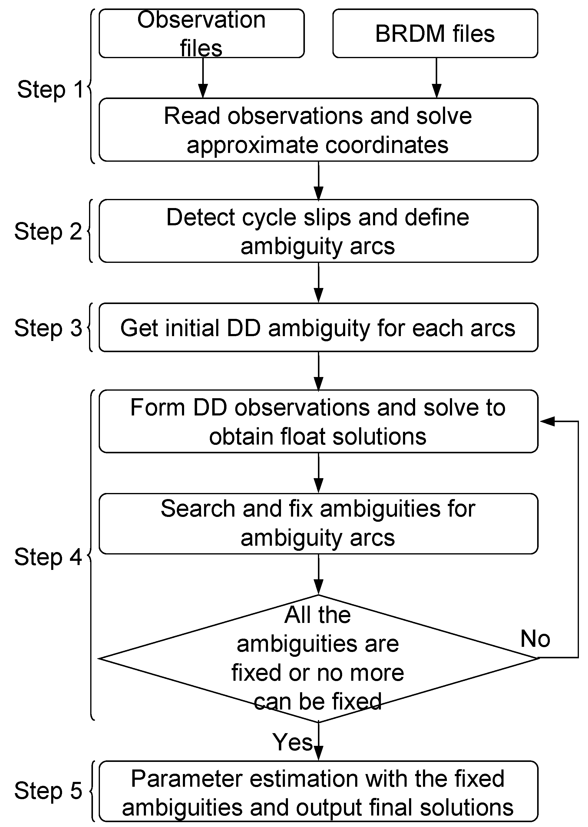
2.3. Data Processing Flowchart

Considering the complexity and imperfection of the inter-system difference method, we will only form the GNSS DD observations within intra-systems. The data processing flowchart is shown in Figure 1.

Step 1:

Read receiver-independent exchange format (RINEX) observations and broadcast ephemeris, transform the original GLONASS carrier phase observations into the basic frequency as shown in (7), and solve the approximate coordinates of a rover station with DD pseudorange IF combinations (PCs).

Step 2:

Detect cycle slips and define ambiguity arcs.

Step 3:

Attain initial DD ambiguity for every ambiguity arc. If GLONASS data are available, the SD ambiguities can also be estimated.

Step 4:

Form DD observations epoch by epoch, solve the resolution with Kalman filtering (KF) to obtain float solutions, and search and fix ambiguities for ambiguity arcs.

Step 5:

Form DD observations, estimate parameters with the fixed ambiguities and use forward and backward KF to smooth the fixed solutions; output the final solutions. The detailed algorithms will be introduced in the following statements.

2.4. Data Pre-Processing and Ambiguity Arc Definition

The data pre-processing involves cycle slip detection and short segment cancellation. In the cycle slip detection procedure, the first-order difference of Melbourne–Wübbena (MW) and geometry-free (GF) combination time series will be employed. The MW and GF combinations are formed as:

$$\{\begin{array}{l}{\phi }_{MW}={\phi }_1-{\phi }_2-\frac{f_1-f_2}{f_1+f_2}(P_1+P_2)\\ {\phi }_{GF}={\phi }_1-\frac{{\lambda }_2}{{\lambda }_1}{\phi }_2\end{array}.$$

(12)

If the difference between adjacent epochs is larger than the threshold (0.25 cycles for GF and 0.5 cycles for MW combinations), an ambiguity flag will be added, and this means an ambiguity arc is ended and another one is started. The new ambiguity arc will be ended at the end of the satellite tracking or another cycle slip epoch. This procedure will be done in the single-differenced observations between stations. Finally, the number of epochs of each ambiguity arc will be counted and the short ones, for example, less than 60 epochs, will be deleted.

2.5. Initial Ambiguity Resolution Using MW+GF Combinations

Before the parameter estimation, we will use MW and GF combinations to calculate the initial ambiguities of the ambiguity arc [23]. The relationship between DD dual-frequency carrier phase ambiguities and DD MW and GF combinations is shown as:

$$\{\begin{array}{l}\nabla \Delta {\phi }_{MW}=\nabla \Delta N_2-\nabla \Delta N_1\\ \nabla \Delta {\phi }_{GF}=\frac{1}{g}\nabla \Delta N_2-\nabla \Delta N_1\end{array},$$

(13)

where $g=\raisebox{1ex}{$f_2$}\!\left/ \!\raisebox{-1ex}{$f_1$}\right.$. Thus, the DD dual-frequency ambiguity can be calculated by:

$$\{\begin{array}{l}\nabla \Delta {\widehat{N}}_1=\frac{1}{g-1}\nabla \Delta {\phi }_{MW}+\frac{g}{g-1}\nabla \Delta {\phi }_{GF}\\ \nabla \Delta {\widehat{N}}_2=\frac{g}{g-1}\nabla \Delta {\phi }_{MW}+\frac{g}{g-1}\nabla \Delta {\phi }_{GF}\end{array}.$$

(14)

In the data processing, the DD MW and GF combinations can be calculated only when the overlapped epochs of the common-viewing station and satellite pairs are over 60, and the estimated ambiguities are flagged at the corresponding non-pivot satellite arc of the rover station. We take a weighted average of the MW and GF combinations of each of the overlapped epochs. According to (14), the dual-frequency float ambiguities can be obtained, and we can get the integer initial ambiguities by rounding them directly as:

$$\{\begin{array}{l}\nabla \Delta {\tilde{N}}_1=round\left(\nabla \Delta {\widehat{N}}_1\right)\\ \nabla \Delta {\tilde{N}}_2=round\left(\nabla \Delta {\widehat{N}}_2\right)\end{array},$$

(15)

where $\nabla \Delta {\tilde{N}}_1$ and $\nabla \Delta {\tilde{N}}_2$ are the initial integer ambiguities. Then, the residuals of MW and GF combinations, $r_{MW}$ and $r_{GF}$, after moving the initial integer ambiguities from (13) will be calculated as:

$$\{\begin{array}{l}{r}_{MW}=\nabla \Delta {\phi }_{MW}^{}-\left(\nabla \Delta {\tilde{N}}_2-\nabla \Delta {\tilde{N}}_1\right)\\ r_{GF}=\nabla \Delta {\phi }_{GF}^{}-\left(\frac{1}{g}\nabla \Delta {\tilde{N}}_2-\nabla \Delta {\tilde{N}}_1\right)\end{array}.$$

(16)

Finally, the RMS statistics of the MW and GF combinations of the DD ambiguity arc, ${\sigma }_{MW}$ and ${\sigma }_{GF}$, will also be calculated and used in the ambiguity resolution procedure.

It should be noted here that the SD ambiguities of GLONASS arcs need to be estimated in this way as well to make the DD GLONASS ambiguities, which are the integer and estimable in (10) and (11).

2.6. Ambiguity Resolution

Before the ambiguity resolution, we firstly estimate the float solutions epoch by epoch using KF. The observation equation of the parameter estimation model can be given as:

$$\begin{array}{cc}v=A{x}_a+B{x}_b+C{x}_u-l,& P\end{array},$$

(17)

where the state vector $x_a$ contains coordinate parameters of rover stations; $x_b$ is the vector for ambiguity parameters and vector $x_u$ includes the other parameters. $v$ denotes the noise vector. $l$ is the OMC (observed minus computed observations). $P$ is the weight matrix of DD observations. $A$, $B$, and $C$ denote the corresponding coefficient matrices of the parameters, respectively. Thus, the estimated states and their coefficient matrices can be written into vectors $x$ and $H$ as:

$$\begin{array}{cc}x={\left[\begin{array}{ccc}{x}_a& x_b& x_u\end{array}\right]}^T& H=\left[\begin{array}{ccc}A& B& C\end{array}\right]\end{array}.$$

(18)

The parameter states and their covariance matrix will be:

$$\{\begin{array}{l}{x}_{e+1}^{-}={\mathsf{\Phi }}_{e+1,e}{x}_e^{+}\\ P_{e+1}^{-}={\mathsf{\Phi }}_{e+1,e}{P}_e^{+}{\mathsf{\Phi }}_{e+1,e}^T+Q_e\end{array},$$

(19)

where $x_e^{+}$ is the a posteriori state vector at epoch e, $x_{e+1}^{-}$ is the a priori state vector at epoch e+1, ${\mathsf{\Phi }}_{e+1,e}$ is the state transition matrix from epoch e to e+1, $P_e^{+}$ is the a posteriori covariance matrix of $x_e^{+}$, $P_{e+1}^{-}$ is the a priori covariance matrix of $x_{e+1}^{-}$, and $Q_e$ is the process noise covariance matrix. The measurement update step is given as:

$$\{\begin{array}{l}{K}_{e+1}=P_{e+1}^{-}{H}_{e+1}^T{\left(H_{e+1}{P}_{e+1}^{-}{H}_{e+1}^T+R_{e+1}\right)}^{-1}\\ x_{e+1}^{+}=x_{e+1}^{-}+K_{e+1}\left(l_{e+1}-H_{e+1}{x}_{e+1}^{-}\right)\\ P_{e+1}^{+}=\left(I_{e+1}-K_{e+1}{H}_{e+1}\right)P_{e+1}^{-}\end{array},$$

(20)

where $K_{e+1}$ is the Kalman gain matrix, $x_{e+1}^{+}$ is the a posteriori parameter state vector at epoch e+1, $l_{e+1}$ is the measurement residual vector, $H_{e+1}$ is the measurement design matrix, $R_{e+1}$ is the measurement noise covariance matrix, and $I_{e+1}$ is an identity matrix. After the parameter estimation in every epoch, an a posteriori residual editing procedure will be carried out to remove the observations whose residuals are 3 times larger than RMS of DD residuals.

In short baselines, the original L1 and L2 observations will be applied and the estimated parameters are the coordinates of the rover station and dual-frequency ambiguities. Meanwhile, the coordinates of the rover station, IF ambiguities, and residual tropospheric delays will be estimated with IF combinations in long baselines.

Assuming that the estimated float L1 and L2 ambiguities of an ambiguity arc are $\nabla \Delta {\widehat{N}}_{f,L1}$ and $\nabla \Delta {\widehat{N}}_{f,L2}$ with the standard deviations ${\sigma }_{L1}$ and ${\sigma }_{L2}$ in short baselines, we firstly sort all the ambiguities in the order of their standard deviations, and then the ambiguity resolution will be started from the smallest ones. If the float ambiguities and their standard deviations satisfy (21), we can round the float ambiguities as to the fixed ones:

$$\{\begin{array}{l}ratio={\left(\frac{1-\left|dL1\right|}{dL1}\right)}^2>relrank\\ ratio={\left(\frac{1-\left|dL2\right|}{dL2}\right)}^2>relrank\\ {\sigma }_{L1}<{\sigma }_t\\ {\sigma }_{L2}<{\sigma }_t\end{array},$$

(21)

where:

$$\{\begin{array}{l}dL1=\nabla \Delta {\widehat{N}}_{f,L1}-round\left(\nabla \Delta {\widehat{N}}_{f,L1}\right)\\ dL2=\nabla \Delta {\widehat{N}}_{f,L2}-round\left(\nabla \Delta {\widehat{N}}_{f,L2}\right)\end{array},$$

(22)

where $relrank$ defaultly with 25 and ${\sigma }_t$ with 0.25 cycles are the thresholds.

In long baselines, the estimated float IF ambiguities and standard deviations are $\nabla \Delta {\widehat{N}}_{f,IF}$ and ${\sigma }_{IF}$. Due to residual orbit errors, tropospheric delays, and the large noise of IF combinations, we need to search the optimal ambiguities for long baselines. The search space for L1 is from ${\chi }_{\min }$ to ${\chi }_{\max }$, and L2 ambiguity is centered on the L1 candidate and takes $\eta$ as steps on both sides of it, as shown in (23). The ways to estimate ${\chi }_{\min }$, ${\chi }_{\max }$, and $\eta$ are shown in (24):

$$\{\begin{array}{l}RL1\in \left[{\chi }_{\min },{\chi }_{\max }\right]\\ RL2\in \left[RL1-\eta ,RL1+\eta \right]\end{array},$$

(23)

$$\{\begin{array}{l}\eta =round\left(\left|{\sigma }_{MW}\right|+\left|{\gamma }_{MW}\right|\right)+1\\ {\chi }_{\max }=round\left(\nabla \Delta {\widehat{N}}_{f,LC}-\beta \eta \right)/\left(\alpha +\beta \right)+1\\ {\chi }_{\min }=round\left(\nabla \Delta {\widehat{N}}_{f,LC}+\beta \eta \right)/\left(\alpha +\beta \right)-1\end{array}.$$

(24)

The candidates will be put into (25) to get the residuals of the IF, MW, and GF combinations. Then, the ambiguity decision process will be based on the residuals to select the best and next best fit values shown in (26) and (27), and is followed by a ratio test using (28). The coefficients $a$ and $b$ in (27) are used to control the effects of MW and GF combinations in the ambiguity resolution. We can adjust $a$ and $b$ to fix more ambiguities and avoid the cases of fixing to wrong ambiguities. Normally, b will be set as 0.1 to reduce the weight of GF combinations in long baselines:

$$\{\begin{array}{l}dIF=\nabla \Delta {\widehat{N}}_{f,IF}-\left(\alpha RL1+\beta RL2\right)\\ dMW=r_{MW}-\left(RL1-RL2\right)\\ dGF=r_{GF}-\left(RL1-\frac{f_1}{f_2}RL2\right)\end{array},$$

(25)

$$\{\begin{array}{l}fi{t}_{IF}={\left(dIF/{\sigma }_{IF}^{}\right)}^2\\ fi{t}_{MW}={\left(dMW/{\sigma }_{MW}^{}\right)}^2\\ fi{t}_{GF}={\left(dGF/{\sigma }_{GF}^{}\right)}^2\end{array},$$

(26)

$$fit=fi{t}_{IF}+a·fi{t}_{MW}+b·fi{t}_{GF},$$

(27)

$$ratio={\left(\frac{next\_fit}{best\_fit}\right)}^2.$$

(28)

If the candidates satisfy all the following conditions, the best candidates will be the fixed ambiguities we searched for. These conditions are: ${\sigma }_{IF}$ and ${\sigma }_{MW}$ lower than 0.25 and 0.5 cycles, respectively; the best_fit value lower than the threshold with 25.0; the ratio larger than the threshold $\xi$:

$$\xi =20/\left(1-e^{\frac{-iter}{5}}\right),$$

(29)

where $iter$ is the iteration. This means that $\xi$ is gradually decreasing to fix more ambiguities with iterations; however, the correctness of ambiguity fixing will also be checked and controlled by the other conditions.

After searching and fixing, the fixed ambiguity(-ies) will be treated as a virtual observation with the weight(s) of 10⁹ to update the KF system following (19) to (20), and then, the updated float-valued ambiguity in the following list with the lowest standard deviation will be searched and fixed as the method introduced until the end of the ambiguity list. Then, the KF estimation will be carried out with the fixed ambiguities to estimate the unfixed ones and to search and fix the float-valued ambiguities again. This procedure will be iterated until all the ambiguities are fixed or no more ambiguities can be fixed, which will be kept as a float in the following resolution. In the last step, the data will be resolved with the fixed ambiguities using forward and backward KF to smooth the solutions. Finally, the results will be outputted.

3. Experimental Analysis

In this section, a group of experiments for collecting static and kinematic data are carried out to evaluate the feasibility of the method proposed above.

3.1. Data Collection and Processing Strategies

In the static data collections, we selected baselines of different lengths that GPS, GLONASS, Galileo, and BDS satellites, which can be observed from the Multi-GNSS Experiment (MGEX) network, and the baseline solutions were resolved using GAMIT software in advance to the reference value for comparison purposes. Since not all the receivers can track the BDS-3 satellites, the BDS data applied here were all from the BDS-2 system. The data spanned one week from 24th March 2019 (day of year (DOY) 83) to 30th March 2019 (DOY 89). The kinematic experimental data came from a bridge monitoring platform and a UAV flying trial. The detailed information of the experimental baselines is shown in

Table 1. Experimental baseline information.

Baselines	Locations of Stations	Length	Statement	Data Length, Sampling Rate
CUTA-CUT0	Curtin, Australia	8.42 m	Static	7 d, 30 s
KIRU-KIR0	Kiruna, Sweden	4.47 km	Static	7 d, 30 s
PERT-CUT0	Perth, Australia	22.41 km	Static	7 d, 30 s
NNOR-PERT	New Norcia, Australia	88.56 km	Static	7 d, 30 s
GAMG-DAEJ	Daejeon, Republic of Korea	102.39 km	Static	7 d, 30 s
SHM2-SHM1	Edinburgh, UK	1528.09 m	Kinematic	1 h, 10 Hz
SHM4-SHM1	Edinburgh, UK	1032.67 m	Kinematic	1 h, 10 Hz
ROVE-RS01	Wuhan, China	-	Kinematic	16 m, 5 Hz

.

Two observation resolution methods can be selected according to the baseline lengths. For the short baselines, we directly used L1+L2 observations to solve the solutions. Otherwise, IF combinations were used for long baselines. The detailed data processing strategies are listed in

Table 2. Data processing strategies.

Models or Parameters	Strategies
Observations	Short baselines: L1+L2; Long baselines: IF combinations. The dual-frequency observations for different systems, GPS: L1/L2, BDS: B1/B2, GLONASS: G1/G2, Galileo: E1/E5a
Signals and tracking modes processed	The tracking approaches for the bands are sorted in the ascending order of selecting priority, and each tracking mode is represented by one letter [24]: GPS L1/L2: C S L X W GLONASS G1/G2: C P Galileo E1: C X Galileo E5a: I Q X BDS B1/B2: I Q X
Cutoff elevation	10°
A priori tropospheric zenith dry/wet delays	Provided by Saastamoinen model [25]. The meteorological parameters are provided by GPT2w model [26]. The mapping function is GMF [27].
Tropospheric parameters	The initial value is zero. The a priori standard deviation is 0.1 m and the variance between epochs is simulated by random walk process, with density 9 × 10−8 m2/s.
PCO and PCV	GNSS satellites and receiver antennas follow igs14_2029.atx
Weighting scheme	Elevation dependent model with ${\sigma }^2=a^2+b^2/{\sin }^2\theta$, where $\theta$ presents the elevation of satellite.
Ephemeris	BRDM combined broadcast ephemeris.

.

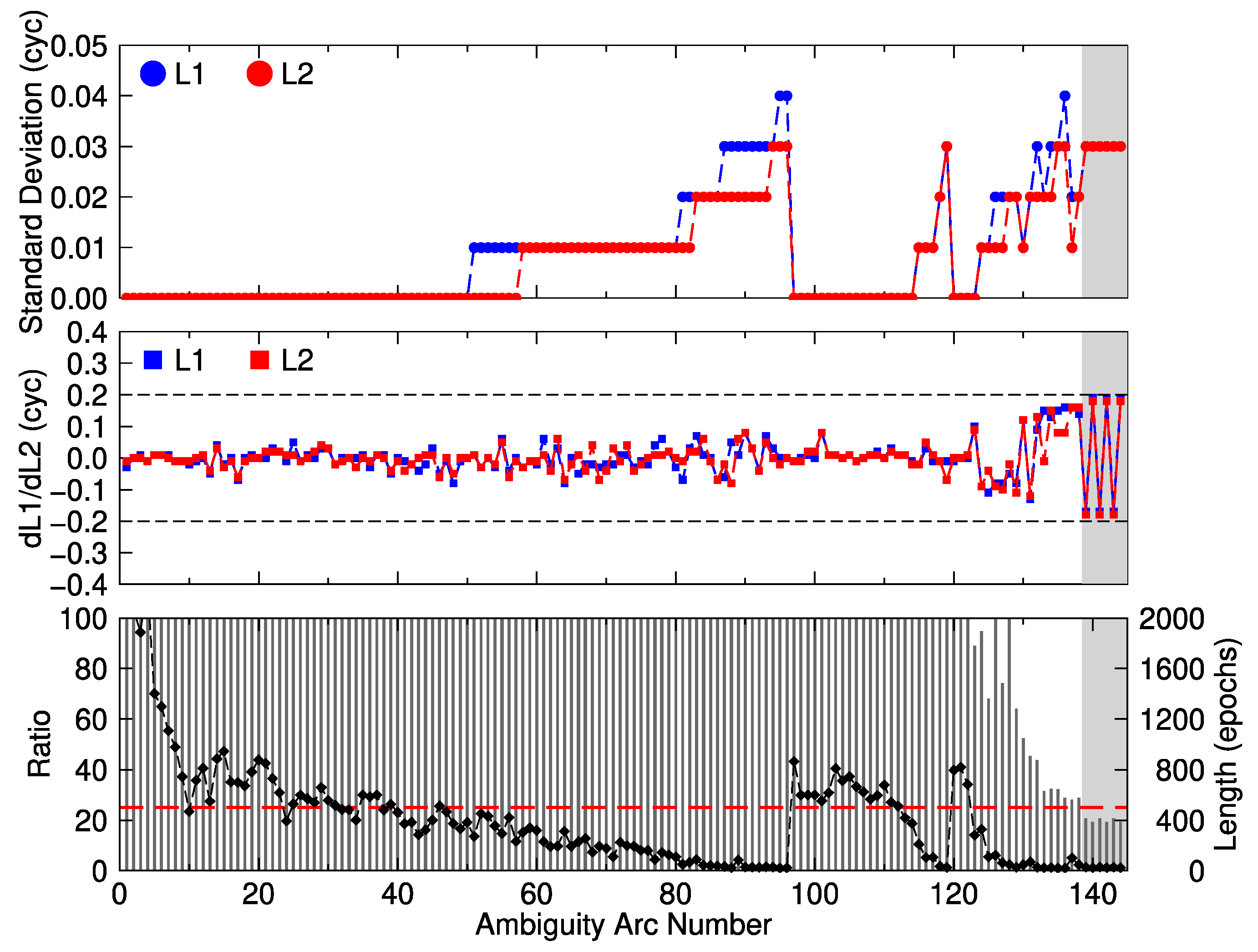
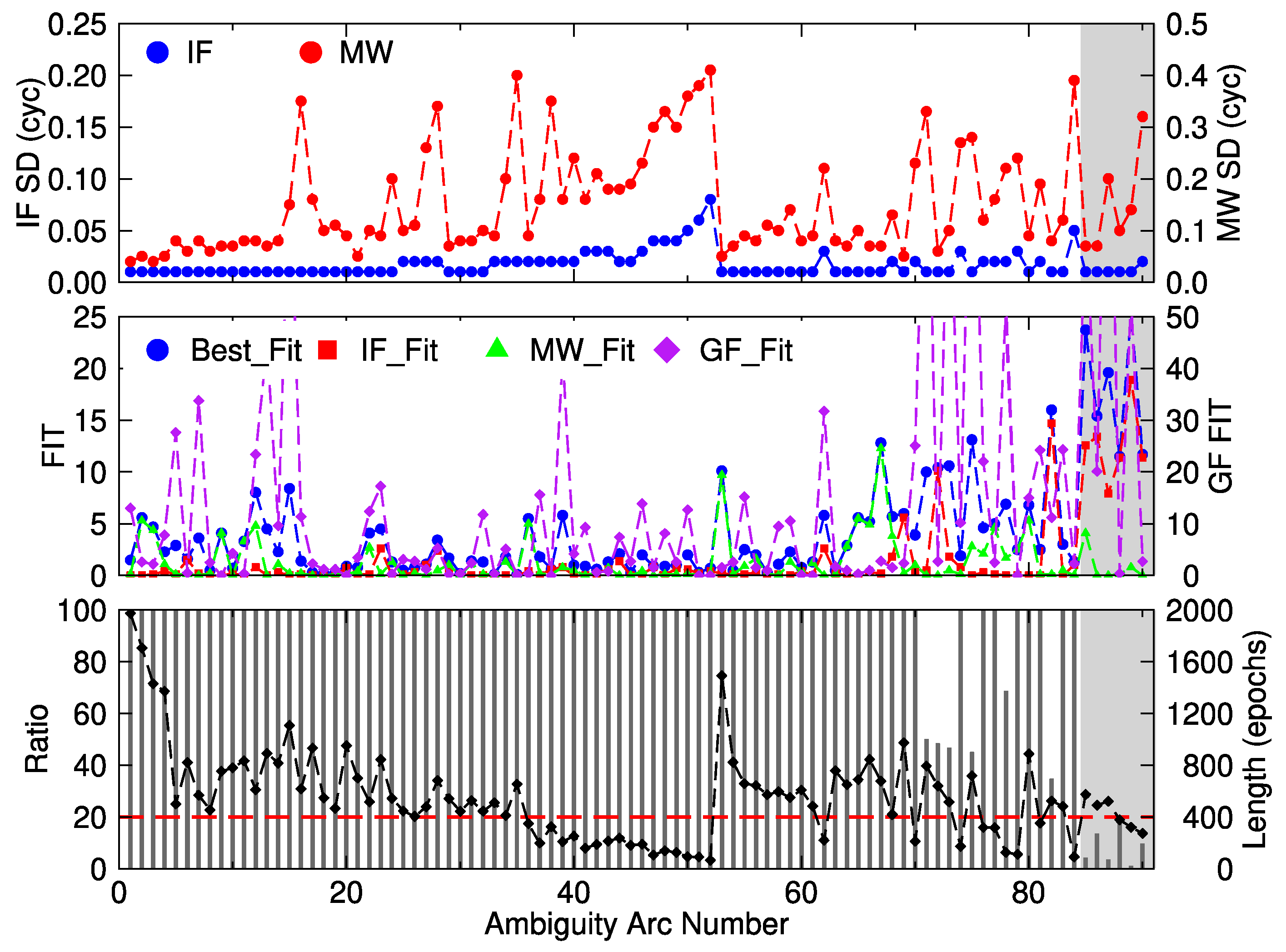
3.2. Ambiguity Resolution

In this section, we will show the performance of ambiguity resolution. Firstly, the statistics of one day of ambiguity resolution will be given in detail for the data processing strategies with L1+L2 and IF observations. Then, the ambiguity-fixing success rate will be analyzed for all daily sessions.

3.2.1. Ambiguity Fixing Performance

Figure 2 and Figure 3 give the detailed statistics of arc ambiguity resolution with L1+L2 and IF observations, respectively, for a whole-day session and the ambiguity arc numbers are listed in the sequence of being fixed. In Figure 2, the standard deviation of the float-valued ambiguities of L1 and L2 are all less than 0.05 cycles, which are significantly lower than the threshold with 0.25 cycles, and the fractional parts of the estimates are confined to within ±0.2 cycles. However, the last few ambiguities show obviously larger values than the previous ones. From the ratio test in the bottom of Figure 2, most of the ratios are much higher than the threshold. The ones with a ratio number of 100 in the figure actually exceed 100, and only 6 out of 144 ambiguities are lower than the threshold. After checking the arc lengths, we know that all of the 6 ambiguity arcs hold only 60–70 epochs, and the elevations are lower than 20°.

Figure 3 shows the conditions that should be satisfied to fix the IF ambiguities in long baselines. The standard deviations of the estimated IF ambiguities and MW combinations are all lower than their corresponding thresholds in the top panel of Figure 3. However, in the middle panel of Figure 3, the fit values of GF combination are relatively larger than IF and MW fit values, especially the last few ambiguities. This is because the GF combinations are significantly affected by the residual ionospheric delays. Hence, we set b in (27) to 0.1 to reduce the weight of the GF combinations in ambiguity resolution. In this case, the fit values of the best fit are all lower than the threshold 25. However, the ratios of 6 ambiguities are all lower than 20 in the iteration, which means they cannot pass the ratio test. By comparing with the fit values, we found that the fittings of these IF ambiguity estimates are also slightly higher than others. This might be due to a poor data quality.

3.2.2. Ambiguity-Fixing Rate

From detailed ambiguity resolution analyses, we list the ambiguity-fixing rate of the daily session for all experiments in

Table 3. Ambiguity resolution success rate statistics (%).

Baselines	Strategy	Sessions (DOY)
		83	84	85	86	87	88	89
CUTA-CUT0	L1+L2	100.0	100.0	100.0	100.0	100.0	100.0	100.0
KIRU-KIR0	L1+L2	100.0	100.0	100.0	100.0	100.0	100.0	100.0
PERT-CUT0	L1+L2	93.24	95.83	96.32	96.96	97.88	95.95	96.18
PERT-CUT0	IF	90.00	93.38	94.53	95.76	96.53	93.65	94.40
NNOR-PERT	IF	91.93	93.33	92.52	91.40	92.34	92.89	90.96
GAMG-DAEJ	IF	92.16	94.48	90.41	92.54	91.43	94.33	91.58
SHM2-SHM1	L1+L2	100.00 (114)
SHM4-SHM1	L1+L2	96.20 (114)
ROV1-RS01	L1+L2	71.76 (88)

. It shows that over 90% of the ambiguities are fixed in the static data experiments, and it is 100% for short baselines. As for PERT-CUT0, the L1+L2 processing strategy is better than the IF combinations in ambiguity resolution. Probably due to the un-eliminable residual ionospheric and tropospheric delays, the ambiguity resolution rate is lower in the long baseline experiments than that of the short ones. However, it could still achieve over 90% in the experiments.

3.3. Static Experimental Analysis

In geophysical research, the kinematic solutions of GNSS permanent stations are applied in general to analyze the daily and sub-daily signals, and further the way they propagate to the annual and semiannual period [28,29]. Besides, the method could also be employed in the monitoring of quasi-static movement of structures, such as dams [30], bridge piers, and geological hazard, etc., to see the spurious signals in the short time scale. Therefore, the positioning precision metrics for different baseline lengths and the corresponding posteriori residual characteristics should be clearly known for an applicable data processing method, software, and engineering application, though we cannot promise the positioning precision in all cases.

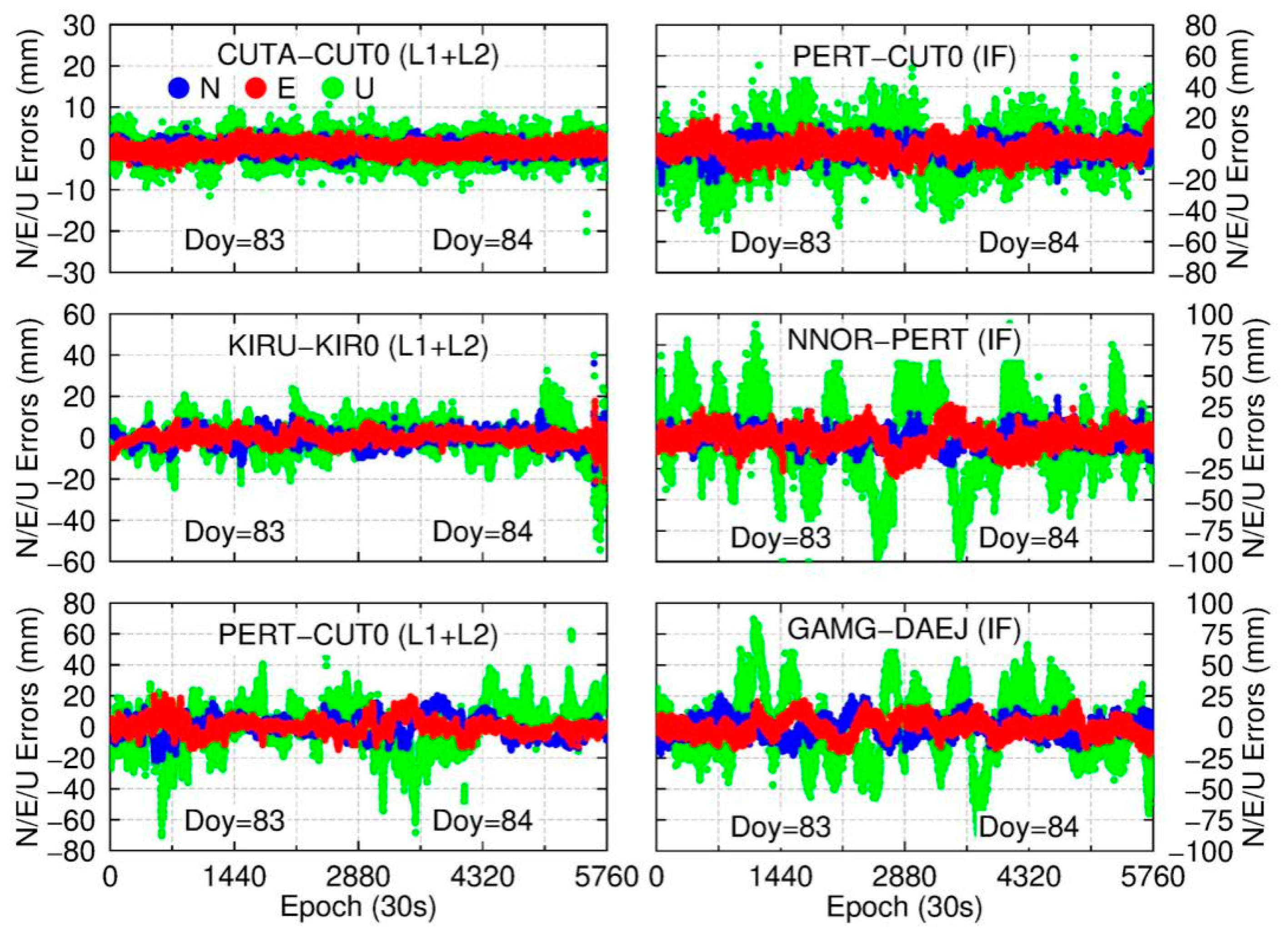
3.3.1. Positioning Results

The results of the baseline resolutions after removing the averages are shown in Figure 4. Due to space limitations, we only show the results for DOY 83 and 84 in 2019. In the baseline time series, the positioning precision is getting worse in all three directions with the increase of the baseline length. However, the fluctuation is always within ±2 cm in the horizontal component. The vertical time series change from only 1 cm for CUTA-CUT0 to almost 1 dm for NNOR-PERT and GAMG-DAEJ.

Table 4. RMS statistics of the baselines resolutions compared with GAMIT solutions (mm).

Baselines and Directions		Session (DOY)
		83	84	85	86	87	88	89
CUTA-CUT0 (L1+L2, 8.42 m)	N	1.2	1.1	1.2	1.4	1.3	1.3	1.3
	E	1.3	1.2	1.2	1.2	1.3	1.4	1.3
	U	3.0	2.8	2.9	3.2	3.0	3.3	3.0
KIRU-KIR0 (L1+L2, 4.47 km)	N	3.4	3.5	2.6	3.9	3.7	3.9	2.9
	E	3.0	2.6	2.2	3.4	3.5	3.4	3.0
	U	7.0	9.3	7.4	8.4	9.2	9.4	8.6
PERT-CUT0 (L1+L2, 22.41 km)	N	5.5	7.7	8.3	7.8	10.3	9.0	6.8
	E	5.4	5.2	5.1	6.4	5.0	5.1	5.2
	U	15.4	16.1	20.4	19.7	20.8	12.7	16.5
PERT-CUT0 (IF, 22.41 km)	N	5.4	5.2	6.7	6.0	6.9	5.0	7.8
	E	5.9	5.2	5.6	5.7	4.7	5.0	5.6
	U	17.5	14.6	17.6	21.3	22.0	15.3	22.4
NNOR-PERT (IF, 88.56 km)	N	6.6	7.1	8.2	7.0	7.6	8.7	9.7
	E	8.0	8.5	7.9	11.3	7.5	7.2	8.8
	U	34.8	32.2	43.1	39.2	31.8	41.3	43.9
GAMG-DAEJ (IF, 102.39 km)	N	8.3	6.4	6.9	8.7	6.8	9.3	7.1
	E	8.0	6.5	7.9	9.9	8.0	6.9	8.8
	U	28.2	25.5	28.3	32.9	32.3	39.0	33.5

shows the RMS statistics of the baseline resolutions compared with the GAMIT solutions. It shows that the precisions of the N and E directions are always better than 10 mm for all baselines. For the baseline length of about 20 km, the results from the L1+L2 observations and IF combinations have similar RMS statistics, with 5–10 mm in the N and E directions and 15–20 mm in the U direction. For the baselines of NNOR-PERT and GAMG-DAEJ, the precisions of the two baselines can achieve to 6–10 mm in the N and E directions, and 30–40 mm in the U direction. The large residual errors in the U directions for the long baselines are probably because of the residual tropospheric delays.

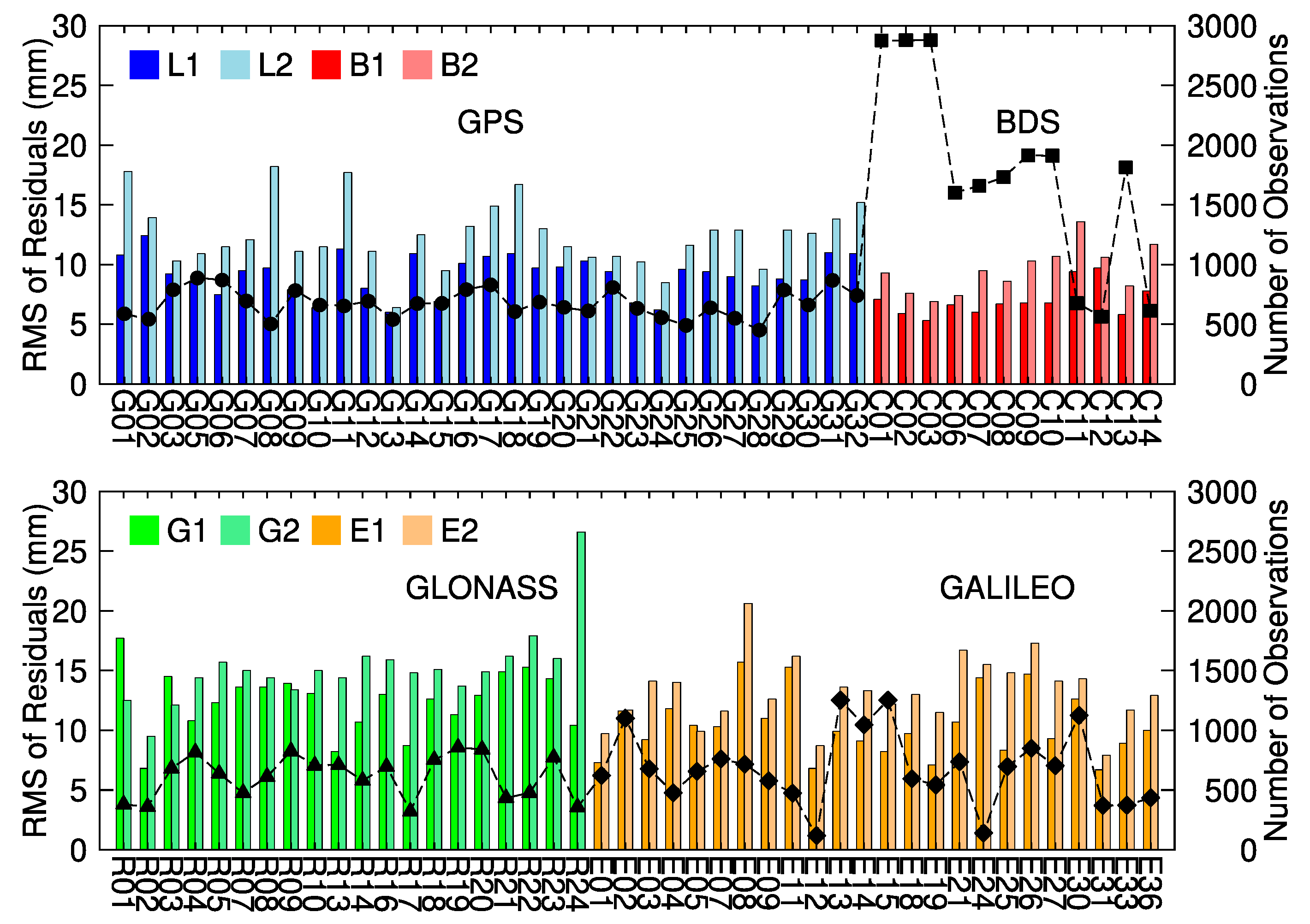
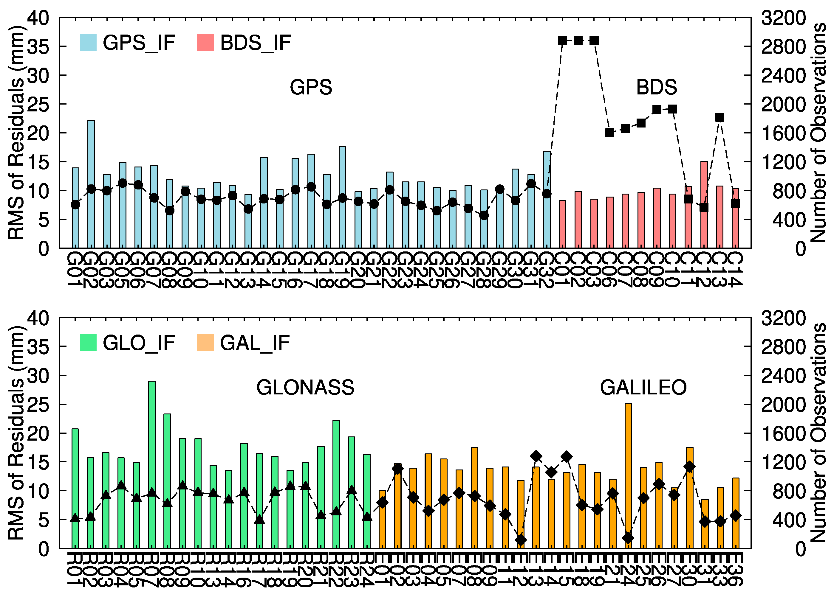
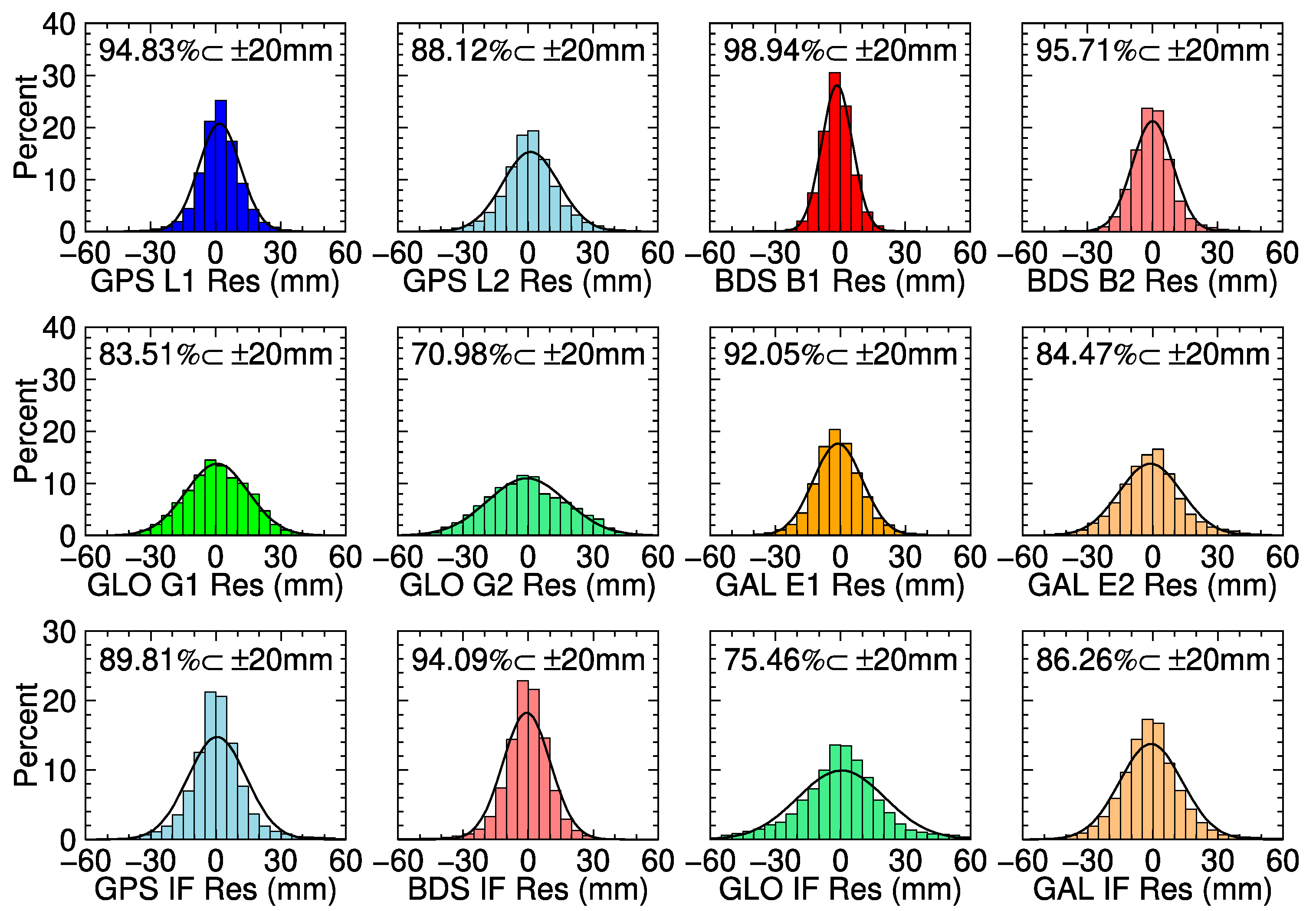
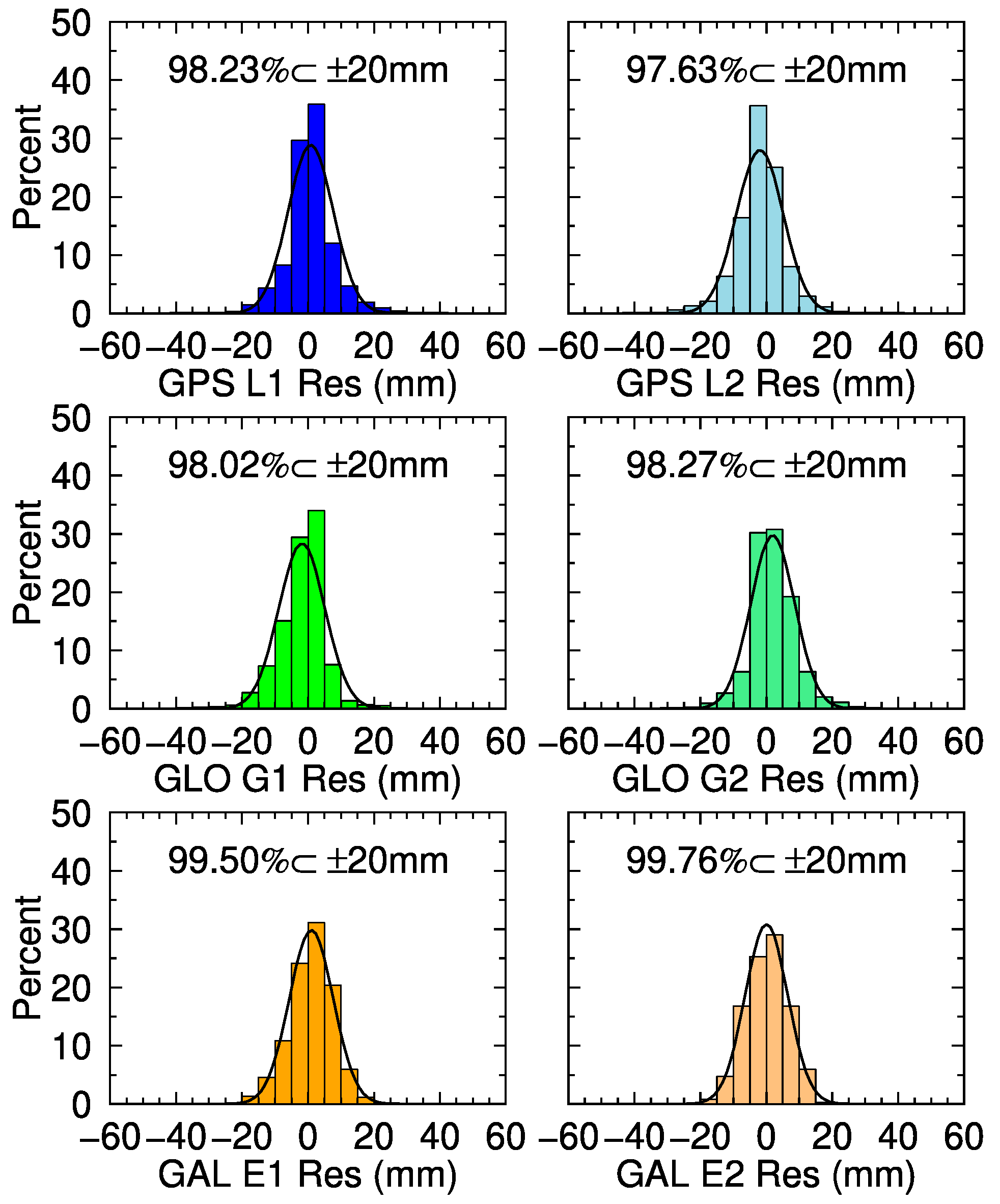
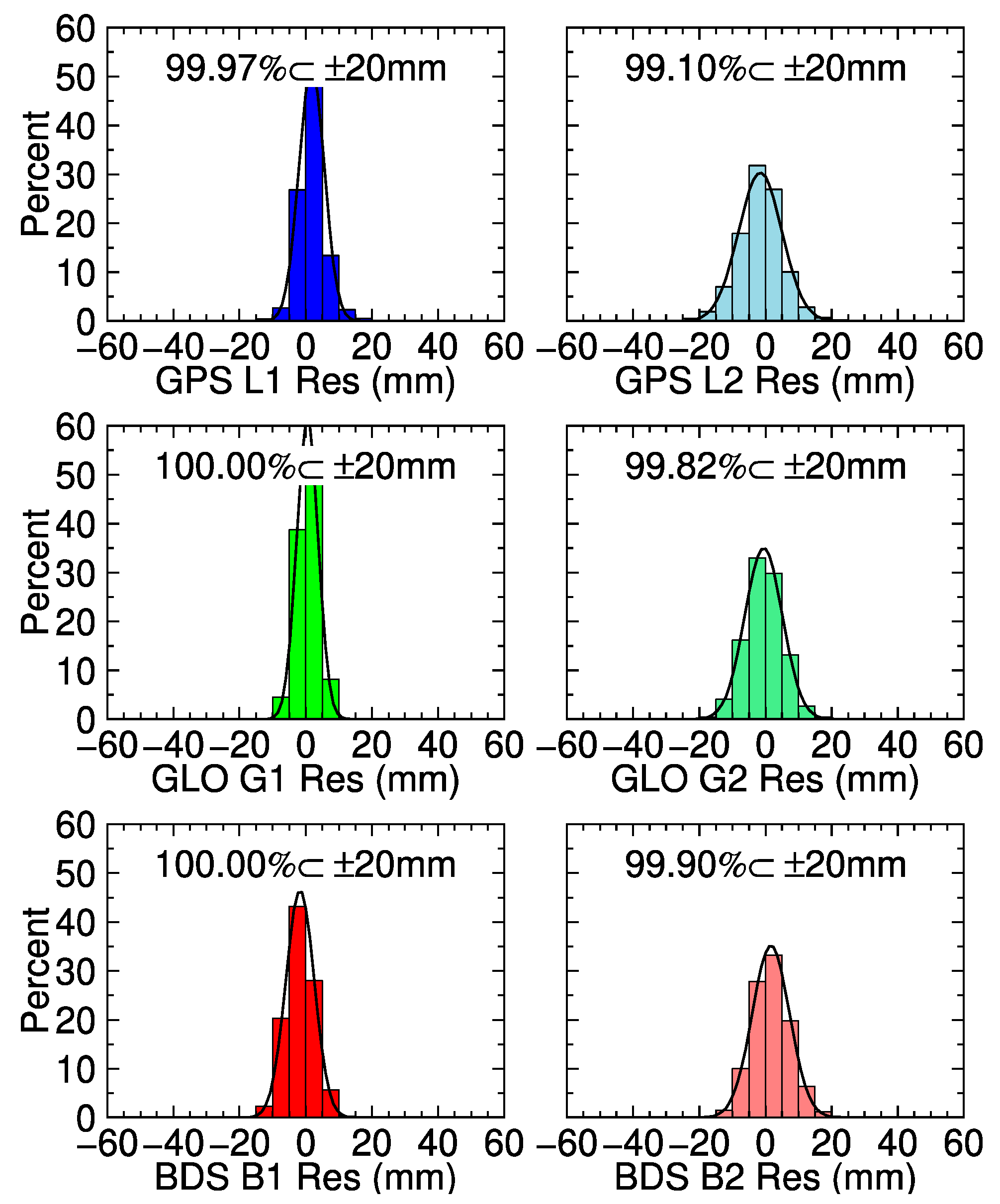
3.3.2. Residual Analysis

Figure 5 and Figure 6 show the residual RMS statistics for every satellite after solving with the L1+L2 observations and IF combinations on DOY 88 for PERT-CUT0. It presents that, mostly, the RMS of satellite residuals is lower than 20 mm. However, they are a little larger than other systems for GLONASS satellites.

Table 5. Means of residual RMS for different GNSS systems (mm).

Baselines	Observation	GPS	BDS	GLONASS	Galileo
CUTA-CUT0	L1	4.1	3.9	5.8	4.1
CUTA-CUT0	L2	4.6	4.0	5.2	4.1
KIRU-KIR0	L1	7.5	7.5	8.6	7.9
KIRU-KIR0	L2	10.0	9.0	11.0	9.8
PERT-CUT0	L1	9.2	7.0	12.4	10.3
PERT-CUT0	L2	12.4	9.5	14.2	13.2
PERT-CUT0	IF	12.8	10.1	14.8	13.9
NNOR-PERT	IF	14.9	13.0	17.3	17.0
GAMG-DAEJ	IF	12.6	13.3	14.7	13.4

demonstrates the averages of the residual RMS for different satellite systems. Apparently, regardless of the positioning with L1+L2 observations and IF combinations, the means of the residual RMS of different systems are all within 20 mm, better than 10 mm for short baselines and 10–20 mm for long baselines. It should be noted that BDS seems to always have the lowest RMS metrics. From the observation numbers, we know that BDS may take the benefits of more observations of the Geostationary Earth Orbits (GEO) and the Inclined GeoSynchronous Orbit (IGSO) satellite.

Figure 7 gives the residual distribution histograms of L1+L2 and IF observations for PERT-CUT0. Basically, over 80% of the residuals of the GPS/BDS/Galileo satellites are within ±2 cm, which is about 0.1 cycles in the carrier phase cycle. The GLONASS one is slightly worse, which is over 70%. Generally, the residuals satisfy the standard normal distribution. For long baselines, however, 80% of GPS and BDS residuals are within ±2 cm, and GLONASS and Galileo are 70%.

3.4. Kinematic Experimental Analysis

In this section, two kinematic experiments, including a bridge monitoring experiment and a UAV flying trial, are carried out to show the performance of this method in the practical applications.

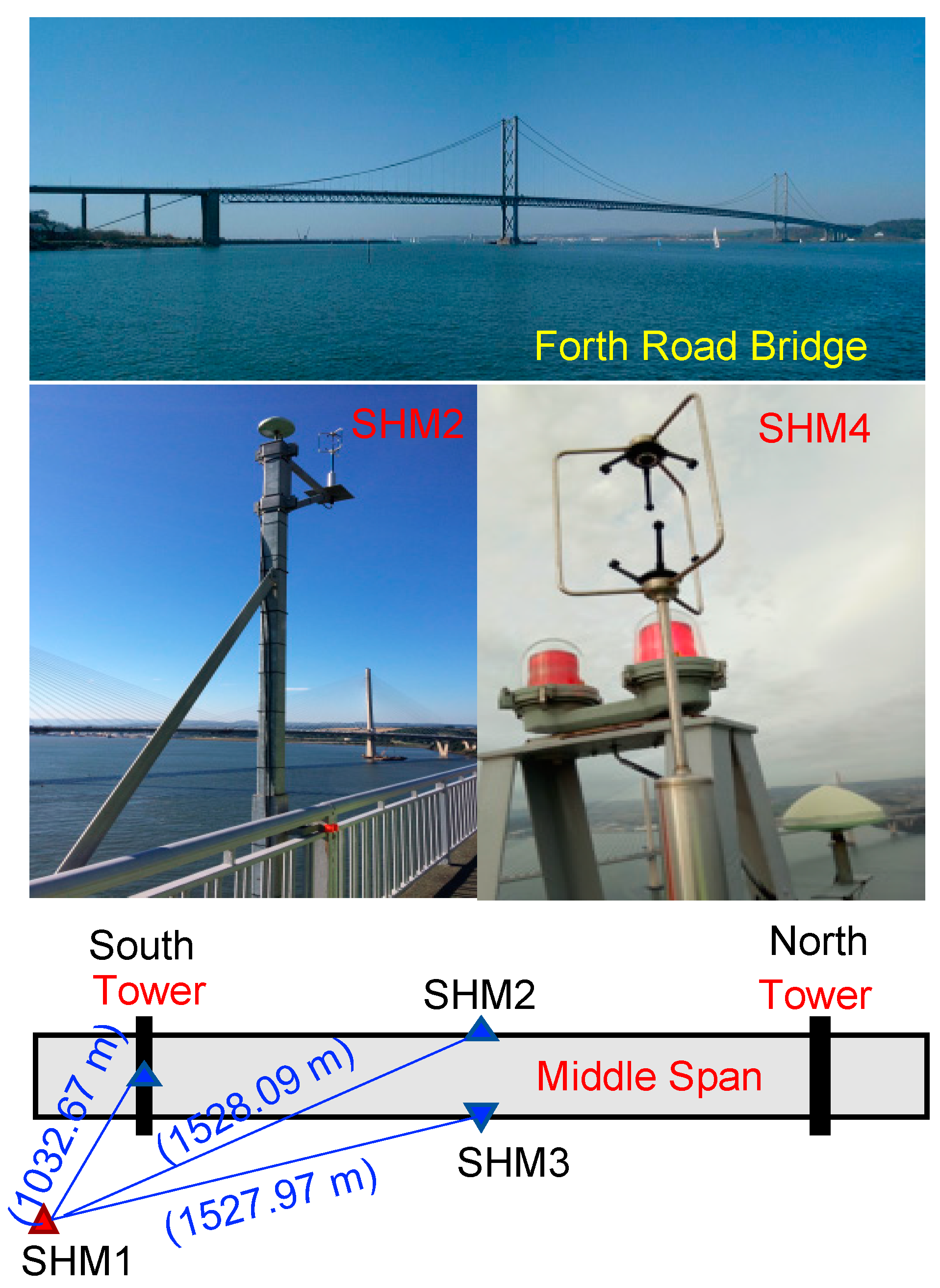
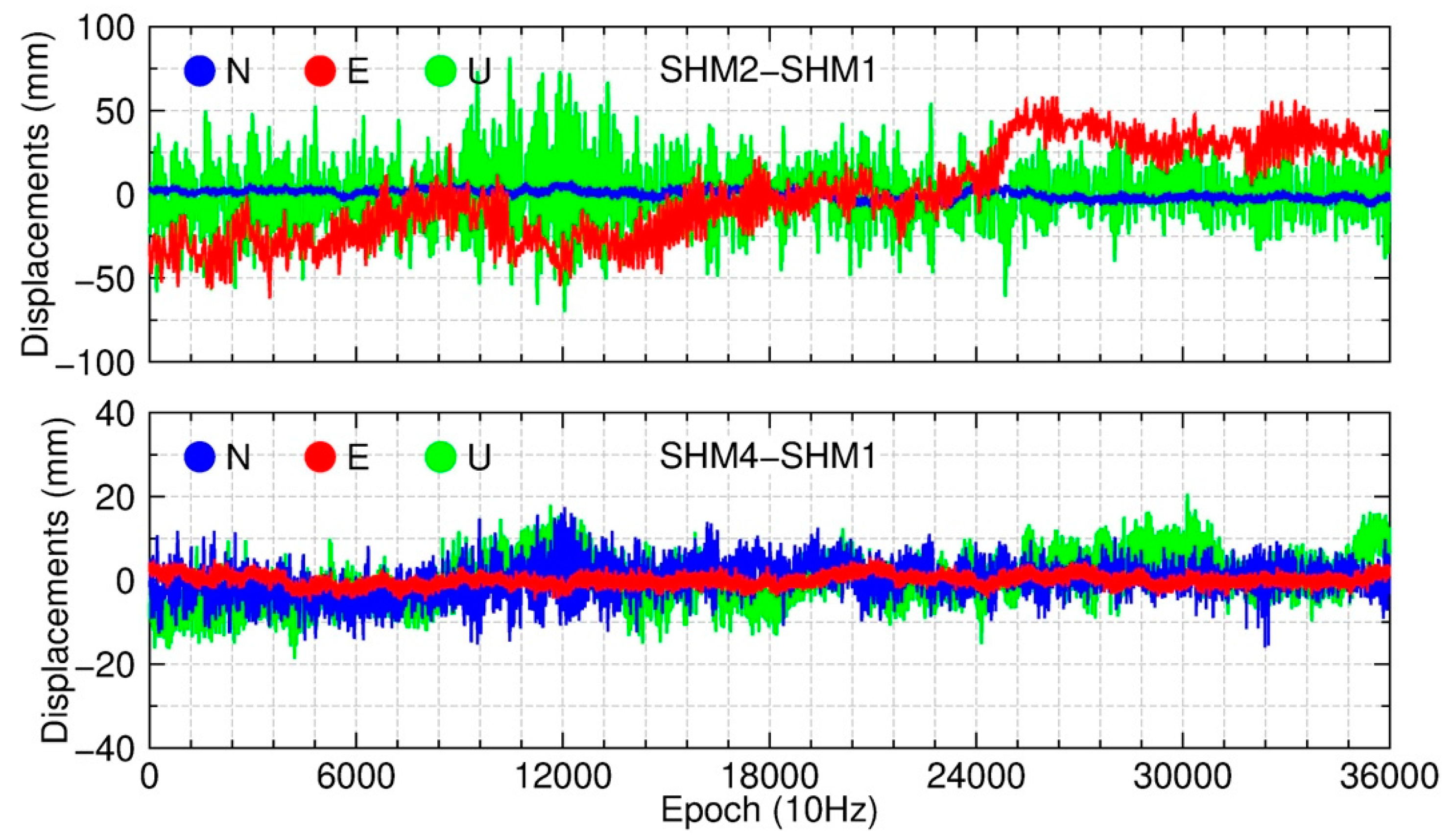
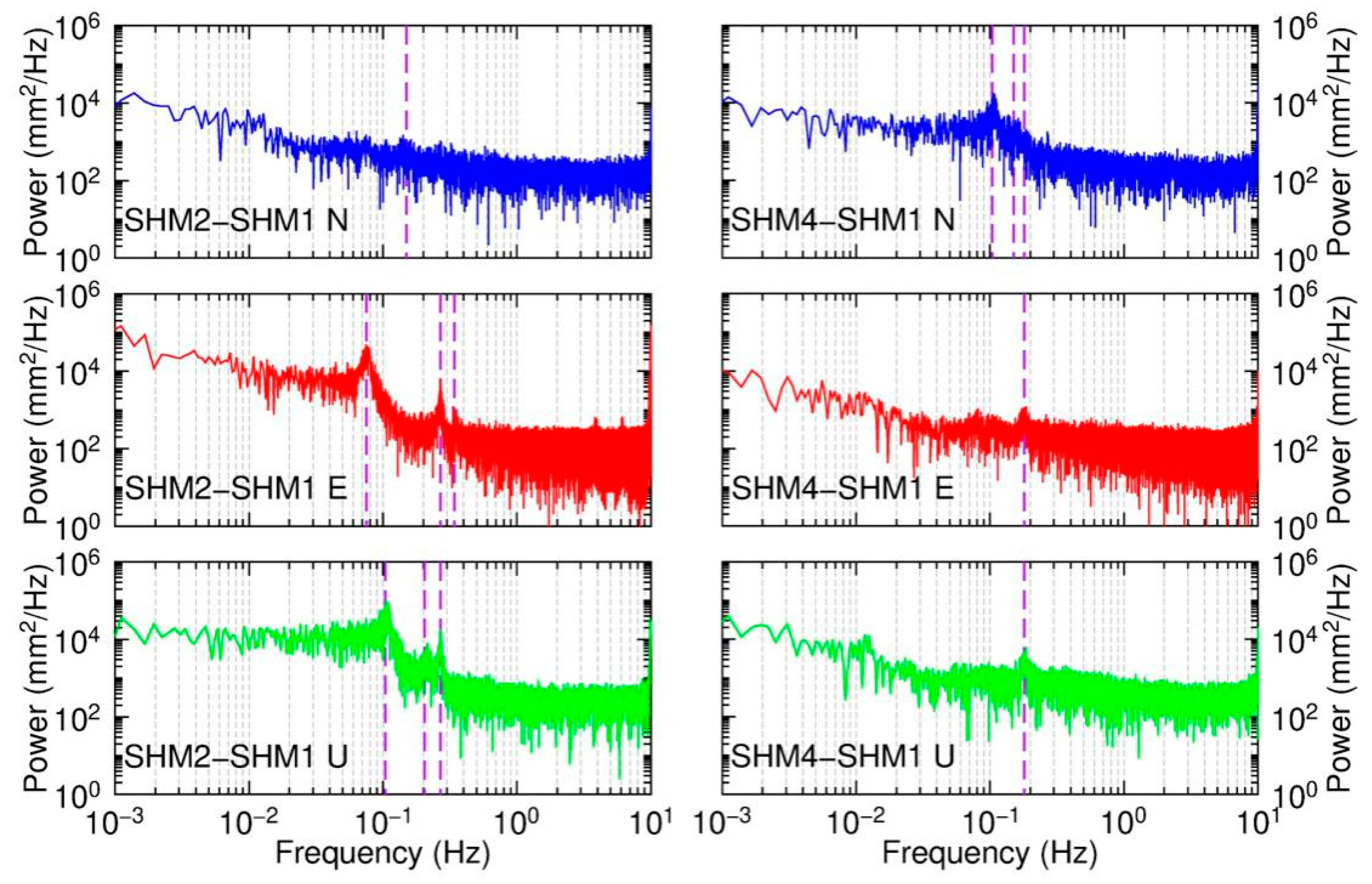
3.4.1. Bridge Monitoring Experimental Analysis

The experimental data were from the GeoSHM (GNSS and Earth Observation for Structural Health Monitoring of Bridges) project, which is led by UbiPOS UK Ltd. and participated in by the University of Nottingham, and other partners under sponsorship from the European Space Agency (ESA). The detailed information about GeoSHM can be found in Meng et al. [6,7,31].

In the GeoSHM system, SHM1 is the reference station. SHM2 and SHM3 are two monitoring stations on both sides of the middle span, and SHM4 is the one sitting on the top of the south tower of the Forth Road Bridge (FRB). They are all equipped with an LEICA GM30 receiver and an LEIAR 10 antenna. Figure 8 depicts the locations of stations on the FRB and the baseline lengths. The data were collected on 24 April 2019 UTC 1:00–2:00. Baselines SHM2-SHM1 and SHM4-SHM1 were selected to test the proposed method. Because only one or two BDS satellites can be tracked in the experiments, the BDS observations were out of our consideration in the data processing.

Figure 9 shows the displacement time series of the monitoring stations. The Forth Road Bridge mostly approaches from the south to the north. Therefore, we will express the baseline resolutions in the bridge local coordinate frame (NEU). N directs the longitude of the bridge, and E directs the lateral direction and U the vertical direction. In the 3-D displacement time series, SHM2 shows the obvious low- and high-frequency movements in the E direction. This is mainly caused by the wind loading. The time series in the N direction is quite stable and the vibration amplitude is larger in the U direction compared with the horizontal directions. However, the time series of SHM4 is stable since it is located on the top of the supporting tower.

Figure 10 shows the spectrum analysis of the displacement time series. The remarkable peak frequencies are illustrated by the purple vertical dash lines and are listed in

Table 6. Peak frequencies extracted from Figure 10 (Hz).

Stations	N	E	U
SHM2	0.15	0.075 0.268 0.342	0.104 0.205 0.268
SHM4	0.104 0.15 0.18	0.18	0.18

. Compared with the results from Meng et al. [7], only the first modal frequency of SHM2 in the E direction is different, with 0.065 Hz in Meng et al. [7]. The possible reason is that the vehicle burden has been relieved as only the public transportations are being permitted to pass through the FRB from the beginning of September 2017. Thus, the modal frequency could have changed under different mass loadings due to traffics. The other frequencies showing the same values as Meng et al. indicates that the method proposed is appropriate for the bridge displacement and vibration monitoring application [7].

The residual distribution histograms are shown in Figure 11. It shows that the residuals of all GNSS systems are basically within ±2 cm and satisfy the standard normal distribution.

In this experiment, 100% of the ambiguities are fixed for SHM2-SHM1 and 96.2% for SHM4-SHM1 from Table 3. Two factors may affect the ambiguity resolution at SHM4-SHM1, including the obstructions beside SHM4 and the height distance between SHM4 and SHM1, which is over 200 m. The large height distance of the two stations could cause residual tropospheric delays, which may not be completely differenced by the DD method.

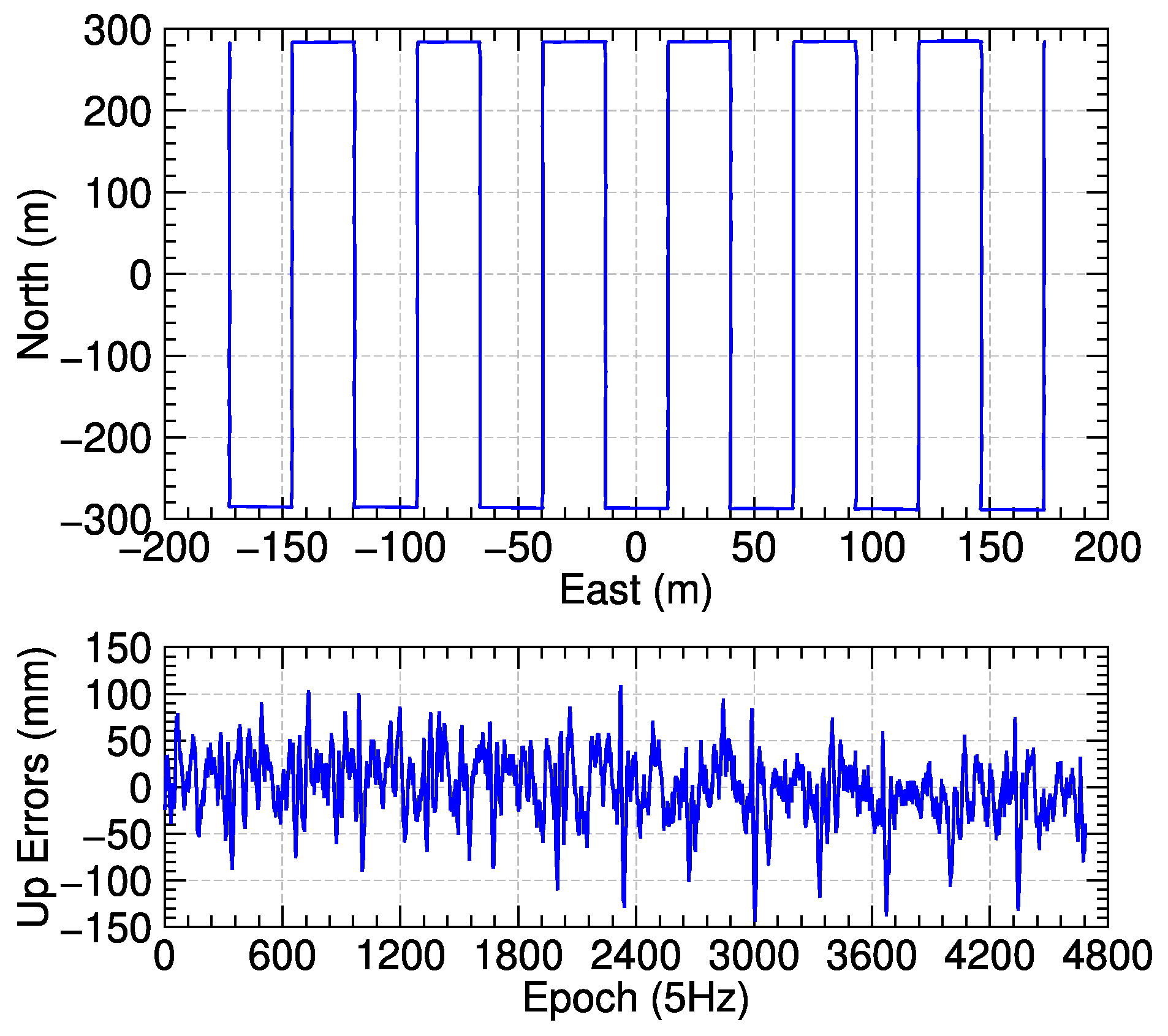
3.4.2. UAV Flying Trial Analysis

The UAV flying trial was carried out at Wuhan University in China on 29 March 2019 (DOY 88). It was a UAV photogrammetry trial. The reference station RS01 is located on the roof of the School of Remote Sensing and Information Engineering, which is equipped with a Hi-Target iRTK2 receiver and an IRTK2-2 antenna. The sampling rate was set to 5 Hz and the cutoff elevation is 10°. The UAV is equipped with a DJI PHANTOM 4 RTK equipment. The trial lasted 16 minutes and the flight altitude was about 150 m. The weather was sunny and breezy during the experiment. We collected the GPS, BDS, and GLONASS observations and there were 4684 epochs in total. Because of the equipment failure, only three to four GLONASS satellites could be tracked during the experiment. Therefore, only three GLONASS satellites were available in the data processing.

Figure 12 shows the UAV trajectory. In the horizontal plane, a clear aerial photogrammetry type stripes can be observed, and the oscillations in the U direction are shown due to the wind effect. When the UAV changes directions, there would be a larger oscillation shown in the U time series with 10–15 cm; otherwise, the oscillations are mostly within 5 cm.

Similarly, Figure 13 gives the residual distribution histograms. The residual RMS values of the satellites are all within 10 mm and the residuals are almost 100% within ±2 cm.

As for the ambiguity resolution in this experiment, only 71.76% of the ambiguities are fixed in Table 3. It is because the observation tracking mode or channel is inconsistent between the base and rover receivers for several GPS satellites. The DD method cannot eliminate the phase hardware delays, which affects the GPS ambiguity resolution. However, all the BDS ambiguities are successfully fixed, which can guarantee the positioning precision.

4. Conclusions

RTK is currently the primary choice in high-precision positioning services. However, it could not always achieve a reliable solution on a harsh environment or even fix wrong ambiguities. A high-precision GNSS data post-processing method is needed to be the back-up solution or augment method to support the numerous geophysical research and geodetic engineering applications. Therefore, we proposed a new multi-GNSS differential phase kinematic post-processing method. We formulated the DD GLONASS phase formulas and demonstrated the arc ambiguity resolution method. Based on the static and kinematic baseline resolutions, the results imply that 100% of the ambiguities in short baselines and over 90% in long baselines can be fixed with the ambiguity resolution method. The positioning precision of better than 10 mm can always be achieved in the horizontal component for the selected baselines, and in the vertical component, with better than 10 mm in short baselines and 30–40 mm in long baselines. In the posterior residual analysis, it was found that the RMS of the residuals for different systems were all better than 10 mm. Mostly, the residuals satisfy the standard normal distribution. Besides, we demonstrated that this method could be used for bridge displacement and vibration monitoring and UAV photogrammetry.

References

1. Benassi, F.; Dall’Asta, E.; Diotri, F.; Forlani, G.; di Cella, U.M.; Roncella, R.; Santise, M. Testing accuracy and repeatability of UAV blocks oriented with GNSS-supported aerial triangulation. Remote Sens. 2017, 9, 172. [Google Scholar] [CrossRef] [Green Version]
2. Forlani, G.; Dall’Asta, E.; Diotri, F.; di Cella, U.M.; Roncella, R.; Santise, M. Quality assessment of DSMs produced from UAV flights georeferenced with on-board RTK positioning. Remote Sens. 2018, 10, 311. [Google Scholar] [CrossRef] [Green Version]
3. Li, W.; Li, W.; Cui, X.; Zhao, S.; Lu, M. A tightly coupled RTK/INS algorithm with ambiguity resolution in the position domain for ground vehicles in harsh urban environments. Sensors 2018, 18, 2160. [Google Scholar] [CrossRef] [PubMed] [Green Version]
4. Meng, X.; Roberts, G.W.; Dodson, A.H.; Cosser, E.; Barnes, J.; Rizos, C. Impact of GPS satellite and pseudolite geometry on structural deformation monitoring: Analytical and empirical studies. J. Geod. 2004, 77, 809–822. [Google Scholar] [CrossRef]
5. Meng, X.; Dodson, A.; Roberts, G.W. Detecting bridge dynamics with GPS and triaxial accelerometers. Eng. Struct. 2007, 29, 3178–3184. [Google Scholar] [CrossRef]
6. Meng, X.; Nguyen, D.; Xie, Y.; Owen, J.; Psimoulis, P.; Ince, S.; Chen, Q.; Ye, J.; Bhatia, P. Design and implementation of a new system for large bridge monitoring—GeoSHM. Sensors 2018, 18, 775. [Google Scholar] [CrossRef] [Green Version]
7. Meng, X.; Xi, R.; Xie, Y. Dynamic characteristic of the forth road bridge estimated with GeoSHM. J. Glob. Position. Syst. 2018, 16, 4. [Google Scholar] [CrossRef]
8. Moschas, F.; Stiros, S. Dynamic multipath in structural bridge monitoring: An experimental approach. GPS Solut. 2014, 18, 209–218. [Google Scholar] [CrossRef]
9. Imparato, D.; El-Mowafy, A.; Rizos, C.; Wang, J. Vulnerabilities in SBAS and RTK positioning in intelligent transport systems: An overview. In Proceedings of the International Global Navigation Satellite System Association IGNSS Symposium, Sydney, Australia, 7–9 February 2018. [Google Scholar]
10. Fan, P.; Li, W.; Cui, X.; Lu, M. Precise and robust RTK-GNSS positioning in urban environments with Dual-antenna configuration. Sensors 2019, 19, 3586. [Google Scholar] [CrossRef] [Green Version]
11. El-Mowafy, A. Analysis of web-based GNSS post-processing services for static and kinematic positioning using short data spans. Surv. Rev. 2011, 43, 535–549. [Google Scholar] [CrossRef] [Green Version]
12. Chen, G. GPS Kinematic Positioning for the Airborne Laser Altimetry at Long Valley, California. Ph.D. Thesis, Massachusetts Institute of Technology, Cambridge, MA, USA, 1998. [Google Scholar]
13. Lu, B.; Jin, J.; Duan, W.; Chen, L.; Guan, H. Research of GPS signal multipath effects based on GAMIT TRACK. Adv. Mater. Res. 2012, 588, 912–919. [Google Scholar] [CrossRef]
14. King, M.; Williams, S. Apparent stability of GPS monumentation from short-baseline time series. J. Geophys. Res. 2009, 114. [Google Scholar] [CrossRef]
15. Moschas, F.; Stiros, S. PLL bandwidth and noise in 100 Hz GPS measurements. GPS Solut. 2015, 19, 173–185. [Google Scholar] [CrossRef]
16. Tiryakioglu, I.; Yigit, C.O.; Yavasoglu, H.; Saka, M.H.; Alkan, R.M. The determination of interseismic, coseismic and postseismic deformations caused by the Gökçeada-Samothraki earthquake (2014, Mw: 6.9) based on GNSS data. J. Afr. Earth Sci. 2017, 133, 86–94. [Google Scholar] [CrossRef]
17. Zrinjski, M.; Barković, Đ.; Matika, K. Razvoj i modernizacija GNSS-a. Geodetski list. 2019, 73, 45–65. [Google Scholar]
18. Teunissen, P.J.G.; Montenbruck, O. Springer Handbook of Global Navigation Satellite Systems; Springer: Berlin, Germany, 2017. [Google Scholar]
19. Teunissen, P.J.G. A new GLONASS FDMA model. GPS Solut. 2019, 23, 100. [Google Scholar] [CrossRef] [Green Version]
20. Leick, A. GLONASS satellite surveying. J. Surv. Eng. 1998, 124, 91–99. [Google Scholar] [CrossRef]
21. Sleewaegen, J.; Simsky, A.; Wilde, W.; Boon, F.; Willems, T. Demystifying GLONASS inter-frequency carrier phase biases. Inside GNSS 2012, 7, 57–61. [Google Scholar]
22. Geng, J.; Zhao, Q.; Shi, C.; Liu, J. A review on the inter-frequency biases of GLONASS carrier-phase data. J. Geod. 2017, 91, 329–340. [Google Scholar] [CrossRef]
23. Xi, R.; Meng, X.; Jiang, W.; An, X.; Chen, Q. GPS/GLONASS carrier phase elevation-dependent stochastic modelling estimation and its application in bridge monitoring. Adv. Space Res. 2018, 62, 2566–2585. [Google Scholar] [CrossRef]
24. Gurtner, W.; Estey, L. RINEX: The Receiver Independent Exchange Format, Version 3.02; Technical Report; IGS Central Bureau: Pasadena, CA, USA, 2013. [Google Scholar]
25. Saastamoinen, J. Atmospheric correction for the troposphere and stratosphere in radio ranging satellites. Use Artif. Satell. Geod. 1972, 15, 247–251. [Google Scholar]
26. Böhm, J.; Möller, G.; Schindelegger, M.; Pain, G.; Weber, R. Development of an improved empirical model for slant delays in the troposphere (GPT2w). GPS Solut. 2015, 19, 433–441. [Google Scholar] [CrossRef] [Green Version]
27. Böhm, J.; Niell, A.; Tregoning, P.; Schuh, H. Global Mapping Function (GMF): A new empirical mapping function based on numerical weather model data. Geophy. Res. Lett. 2006, 33, L07304. [Google Scholar] [CrossRef] [Green Version]
28. King, M.; Watson, C.; Penna, N.; Clarke, P. Subdaily signals in GPS observations and their effect at semiannual and annual periods. Geophys. Res. Lett. 2008, 35, L03302. [Google Scholar] [CrossRef] [Green Version]
29. King, M.; Watson, C. Long GPS coordinate time series: Multipath and geometry effects. J. Geophys. Res. Sol. Earth 2010, 115, B4. [Google Scholar] [CrossRef]
30. Xi, R.; Zhou, X.; Jiang, W.; Chen, Q. Simultaneous estimation of dam displacements and reservoir level variation from GPS measurements. Measurement 2018, 122, 247–256. [Google Scholar] [CrossRef]
31. Meng, X.; Nguyen, D.; Owen, J.; Xie, Y.; Psimoulis, P.; Ye, G. Application of GeoSHM System in Monitoring Extreme Wind Events at the Forth Road Bridge. Remote Sens. 2019, 11, 2799. [Google Scholar] [CrossRef] [Green Version]
Figure 1. Data processing flowchart.
Remotesensing 12 02727 g001
Figure 2. Ambiguity resolution of each arc with L1+L2 observations. The experimental data is from PERT-CUT0 on DOY 84 2019. The top panel shows the standard deviations of the float ambiguity estimates of L1 and L2. The middle panel indicates the fractional part of the float ambiguity estimates, and the bottom one presents the lower ratio value of L1 and L2 estimates in (24). The red dash line indicates the threshold. The diamond symbol denotes the length of the arc referring to the right vertical axis. The gray background means the unfixed ambiguity arcs.
Remotesensing 12 02727 g002
Figure 3. Ambiguity resolution of each arc with IF observations. The experimental data is from NNOR-PERT on DOY 84 2019. The top panel shows the standard deviations of the IF estimates referring to the left axis and the MW combinations to the right. The middle panel denotes the fit values computed with (26) and (27). Notes the axis of GF fit values is shown on the right. In the bottom, the ratio values calculated with (28) are shown. The red dash line indicates the lowest threshold of 20. The diamond symbols denote the length of the arc referring to the right vertical axis. The gray background means the unfixed ambiguity arcs.
Remotesensing 12 02727 g003
Figure 4. Residual time series of baseline resolutions after removing averages. Notes the scale ranges of the panels are different.
Remotesensing 12 02727 g004
Figure 5. The posteriori residual RMS and the observation number statistics of GNSS satellites for PERT-CUT0 after solving with L1+L2 observations on DOY 88.
Remotesensing 12 02727 g005
Figure 6. The posteriori residual RMS and the observation number statistics of GNSS satellites for PERT-CUT0 after solving with IF combinations on DOY 88.
Remotesensing 12 02727 g006
Figure 7. Residual distribution histograms of PERT-CUT0 after solving with the L1+L2 observations and IF combinations on DOY 88. The top and middle panels denote the residuals of L1 and L2. The bottom panel shows the IF residuals. The black curve denotes a fitted normal distribution, and means “within”.
Remotesensing 12 02727 g007
Figure 8. The landscape of the FRB, antenna set-ups with baseline lengths and the observation environment of the SHM2 and SHM4 stations.
Remotesensing 12 02727 g008
Figure 9. Displacement time series of SHM2 and SHM4.
Remotesensing 12 02727 g009
Figure 10. The spectrum analysis of vibrations of SHM2 and SHM4. The purple vertical dash lines indicate the locations of peak frequencies.
Remotesensing 12 02727 g010
Figure 11. Distribution histogram of residuals for SHM2-SHM1.
Remotesensing 12 02727 g011
Figure 12. Trajectory of the UAV after data processing.
Remotesensing 12 02727 g012
Figure 13. Distribution histograms of the residuals after data processing for the UAV flying trial.
Remotesensing 12 02727 g013