Article

An SBAS Integrity Model to Overbound Residuals of Higher-Order Ionospheric Effects in the Ionosphere-Free Linear Combination

1
Galileo Competence Center, German Aerospace Center, Kalkhorstweg 53, 17235 Neustrelitz, Germany
2
Institute for Solar-Terrestrial Physics, German Aerospace Center, Kalkhorstweg 53, 17235 Neustrelitz, Germany
*
Author to whom correspondence should be addressed.
Remote Sens. 2020, 12(15), 2467; https://doi.org/10.3390/rs12152467
Submission received: 29 June 2020 / Revised: 29 July 2020 / Accepted: 29 July 2020 / Published: 31 July 2020
(This article belongs to the Special Issue Remote Sensing of Ionosphere Observation and Investigation)

Abstract

:
The next generation of satellite-based augmentation systems (SBAS) will support aviation receivers that take advantage of the ionosphere-free dual-frequency combination. By combining signals of the L1 and L5 bands, about 99% of the ionospheric refraction effects on the GNSS (Global Navigation Satellite Systems) signals can be removed in the user receivers without additional SBAS corrections. Nevertheless, even if most of the negative impacts on GNSS signals are removed by the ionospheric-free combination, some residuals remain and have to be taken into account by overbounding models in the integrity computation conducted by safety-of-live (SoL) receivers in airplanes. Such models have to overbound residuals as well, which result from the most rare extreme ionospheric events, e.g., such as the famous “Halloween Storm”, and should thus include the tails of the error distribution. Their application shall lead to safe error bounds on the user position and allow the computation of protection levels for the horizontal and vertical position errors. Here, we propose and justify such an overbounding model for residual ionospheric delays that remain after the application of the ionospheric-free linear combination. The model takes into account second- and third-order ionospheric refraction effects, excess path due to ray bending, and increased ionospheric total electron content (TEC) along the signal path due to ray bending.

1. Introduction

Airplanes need to rely on ground-based radio systems such as the instrument landing systems (ILS) or satellite-based augmentation systems (SBAS) to be able to perform precise landing operations independent of the weather conditions. Given the fact that SBAS, similar to the European Geostationary Overlay System (EGNOS) or the American Wide Area Augmentation System (WAAS, allow an efficient use of airspace without maintenance or calibration cost for airports, more and more airports are already taking advantage of this technology based on GNSS (Global Navigation Satellite System). (For instance, according to the official website of the FAA (Federal Aviation Administration, already 4053 WAAS procedures are currently (21 May 2020) implemented in 1956 US airports.).
However, ionospheric effects on trans-ionospheric GNSS signals are significant and should not be ignored. The ionospheric propagation effects degrade the true range measurements, whereas the ionospheric irregularities may cause signal loss due to rapid fluctuation of the signals, which is also known as ionospheric scintillation. Signal fluctuations may cause cycle slips; however, if these cycle slips are detected, precise navigation can be achieved under scintillation conditions [1]. Tiwari and Strangeways [2] presented an approach to mitigate the effect of ionospheric scintillation on GNSS users in the European region using total electron content at 1 Hz rate. Demyanov et al. [3] found degradation in the single-frequency WAAS services during geomagnetic storm conditions.
Fortunately, the next generation will not only support single-frequency receivers but also aviation receivers that benefit from the ionospheric-free dual-frequency combination. By combining signals of the L1 and L5 bands, future users will be able to remove about 99% of the ionospheric refraction effects on the GNSS signals instantaneously in the receivers on board the airplane. Thus, this technique will help to significantly increase the service performances of SBAS, in particular for polar and equatorial latitudes where geomagnetic storms or strong ionospheric gradients accompanied by phase and amplitude scintillations may lead to partial losses of the service availability. However, even if most of the negative impacts on GNSS signals are removed by this combination, some residuals remain. They will need to be taken into account in the protection level computation conducted within aircraft receivers by the use of so-called “overbounding models”. Such models overbound residuals also, which result from most rare extreme ionospheric events such as the famous “Halloween Storm” and should thus include the tails of the error distribution. Their application shall lead to safe error bounds on the user position and allow the computation of protection levels for the horizontal and vertical position errors.
Brunner and Gu [4], Bassiri and Hajj [5], and Jakowski et al. [6] were among the first to compute higher-order ionospheric effects in GPS dual frequency combinations. Later, Kedar et al. [7], Fritsche et al. [8], and Hernández-Pajares et al. [9] studied the second-order effect on receiver positions, satellite clocks, and orbits. They found a global southward displacement of several millimeters in the station positions. Hoque and Jakowski [10,11,12,13] derived different approximation formulas to correct the second- and third-order terms in the refractive index, errors due to geometric bending, and differential slant total electron content (TEC) bending effects on geometric range estimation. A comprehensive summary of higher-order effects on geodetic quantities considering all relevant higher-order contributions can be found in Hernández-Pajares et al. [14].
Hadas et al. [15] investigated the impact of the second- and third-order terms, geometric bending effects on satellite orbits, satellite clock corrections, receiver positions, etc. They found that the satellite-related products captured most of the impact of higher-order corrections with the magnitude up to 2 cm for clock corrections. Zhang et al. [16] investigated the impact of higher-order ionospheric effects on tropospheric delay estimation using GNSS observations from about 100 worldwide ground stations. They found that the tropospheric zenith wet delay (ZWD) estimation is affected up to 20 mm during ionospheric and geomagnetic storms. Cai et al. [17] used a quad-constellation (GPS, GLONASS, BDS and Galileo) precise point positioning (PPP) approach for investigating higher-order ionospheric impact in the position domain. They found that higher-order ionospheric terms can affect the 3D position solutions of the quad-constellation PPP up to 6 mm.
Here, we propose and justify a simple overbounding model that bounds ionospheric-free residual delays and can be used for the calculation of the protection levels of an airplane. The model is particularly designed for the “Minimum Operational Performance Standards for Galileo–Global Positioning System–Satellite-Based Augmentation System Airborne Equipment” [18]. The model takes into account the second- and third-order ionospheric refraction effects, excess path due to ray bending, and increased ionospheric TEC along the signal path due to ray bending (the impact of phase and code noises are not part of the model).
The design of the model is very much driven by constrains of the aviation users. The requirements are:
  • the model shall basically overbound any ionospheric-free higher-order residual everywhere for static and dynamic users;
  • the model shall be easy to implement in an aviation receiver and self-standing in terms of not relying on external parameters;
  • the model does not have to provide realistic data in terms of the real characteristics of the ionosphere, as long as it is overbounding the residuals and the maximum values of the model do not jeopardize the error budget of the future aviation user.
The overbounding model is developed by a method that can be seen as an educated guess, combining theoretical knowledge with a number of extreme assumptions on some physical parameters. This approach is chosen because the model will be hard coded in the user receiver, and we have to assure that our model overbounds anomalous ionospheric delays even for the future. This is quite different to single-frequency SBAS. There, the SBAS itself generates the ionospheric error bounds for the user with respect to the broadcast user corrections. This approach allows the post-adoption of the models for the ionospheric threat space based on continuous monitoring activities. For a more detailed overview on SBAS safety assessment guidance related to anomalous ionospheric conditions, we refer to [19].
Moreover, one has to keep in mind that the alert limits for positioning errors for CAT-I landing operations are 40 m for the horizontal errors and 12 m for the vertical errors. Given the fact that the first-order ionospheric effects, which are substantially contributing to the error budget in the single- frequency case are removed, statistical uncertainty can be compensated by putting additional safety margins on the assumptions that are the foundation of the overbounding model.
The baseline criteria to design an overbounding model according to the above listed requirements are:
  • to design the model, using an almost deterministic approach grounded on physical equations;
  • to define input parameters for the equations that are beyond what has been reported in the literature or close to the most extreme values (to estimate representative values, with a very low occurrence probability all over the globe and under all solar conditions would be most likely impossible for an environment as complex as the ionosphere);
  • to put additional margins on the input parameter, taking into account that there may be rare events that are never observed by scientists (such as what has been named a Black Swan by the risk analyst Nassim Nicolas Taleb [20]), but ensuring that the conservatism of the model does not destroy the overall bounding;
  • to validate the model in a multi-dimensional approach to ensure that the mapping function and the approximations, inherent in some of the equation used, are not destroying the overbounding of the model or leading to modeling errors.
The first section gives a brief overview of the impact of ionospheric refraction effects on GNSS signals, followed by a mathematical description of the residuals in the ionospheric-free combination. After a short section on the impact of carrier smoothing on the residuals, we detail the design and justification of the overbounding model according to the strategy that has been detailed above. The subsequent sections describe the ray-tracing results, verifying that the used approximation to compute the third-order residuals and imprecisions introduced by the use of the mapping function do not lead to a violation of the conservativeness of the model. Finally, the paper is closed by a brief summary.

2. Materials and Methods

2.1. Ionospheric Refraction Impacts on Signal Propagation

Ionospheric effects on radio signals can be mathematically formulated as the expansion of the Appleton–Hartree formula [21]. In consideration of different propagation velocities for a single phase carrier and a wave group, the observables for GNSS code (Ψ) and carrier-phase (Φ) observations can be expressed in the dimension of length [22] by the following equations:
Ψ i = ρ + p f i 2 + q f i 3 + t f i 4 + + d i b ( l e n g t h ) ,
Φ i = ρ p f i 2 q 2 f i 3 t 3 f i 4 n i λ i + d i b ( l e n g t h ) .
Here, the index i refer to the GNSS carrier frequency, e.g., L1 or L5. The parameters Ψ and Φ are the measured code and carrier phase ranges, respectively. λ is the corresponding wavelength, and n is the integer ambiguity. ρ corresponds to the geometrical distance plus clock errors and non-ionospheric delays. The quantity d i b ( l e n g t h ) denotes the error contribution of the excess path length due to geometric bending of the signal within the ionosphere. In both equations, the first-order term is related to as f2, the second-order term is related to as f3, and the third-order term is related to as f4. Other error sources such as carrier phase ambiguities, satellite and receiver instrumental biases, multipath effects, and measurements errors are omitted for simplicity in the formulas. The ionosphere-related parameters p, q, and t in (1) and (2) are given by:
p = 40.3   n e   d s = 40.3   ( T E C L o S + T E C b e n d ) ,
q = 2.2566 × 10 12   n e B c o s Θ   d s ,
t = 2437     n e 2   d s + 4.74 × 10 22     n e B 2   ( 1 + c o s 2   Θ ) d s .
Here, ne denotes the electron density and s denotes the signal propagation path. TECLoS is the total electron content (TEC) along the line of sight between receiver and satellite. TECbend is the TEC deviation due to the difference between the real curved ray path and the ray path along the straight line of sight. TECbend is not removed by the ionospheric-free combination, because the ray path is individual for every frequency. B is the magnetic induction, and Θ is the angle of intersection between the Earth’s magnetic field vector and the propagation direction of the transmitted signal. The International System of Units (SI) is used when computing each variable.
To determine the geometric bending term b(length) and TECbend, we use the formulas proposed by Hoque and Jakowski [13]:
d i b ( l e n g t h ) = b 1 f i 4   ( 1 1 b 2   c o s 2   β 1 )   T E C L o S 2 ,
T E C b e n d = 1.11 × 10 3 e x p ( 2.184   β ) T E C L o S 2 f 2   H   ( h m F 2 ) 0.3 .
In (6), b1 = 2.9344×10⁷ and b2 = 0.8260 are model coefficients, and β is the elevation angle in radians. Here, the signal frequency f is in MHz and b(length) is in centimeters. Equation (7) computes TECbend in TECU, H is the atmospheric scale height in km, hmF2 is the maximum ionization height in km, and TECLoS has to be in TECU, β again is in radians, and f isin GHz.
According to Bassiri and Hajj [5], the second term of the ionospheric parameter t leads just to a sub-millimeter range bias for GHz frequencies, and the same appears in terms of higher order. Consequently, these terms will be neglected in the following sections [8,23,24].

2.2. Residuals in the Ionospheric-Free Combination

The ionospheric-free combination for the code and carrier phase (in units of length) on fi and fj frequency (fi > fj) is given by:
f i 2 Ψ i f i 2 f j 2 f j 2 Ψ j f i 2 f j 2 =   ρ Δ s b ( T E C ) 2 Δ s 2 3 Δ s 3 Δ s b ( l e n g t h ) ,
f i 2 Φ i f i 2 f j 2 f 2 2 Φ 2 f i 2 f j 2 =   ρ + Δ s b ( T E C ) + Δ s 2 + Δ s 3 Δ s b ( l e n g t h ) + A i f c ,
where
Δ s b ( T E C ) = 40.3   ( T E C j b e n d T E C i b e n d ) ( f i 2 f j 2 ) ,
Δ s 2 = q 2 f i   f j   ( f i + f j ) ,
Δ s 3 = t 3 f i 2   f j 2 ,
Δ s b ( l e n g t h ) = d j b ( l e n g t h ) f j 2 d i b ( l e n g t h ) f i 2 ( f i 2 f j 2 ) .
Here, Δsb(TEC) denotes residual excess TEC caused by the difference in ray bending of the two combined signals indexed by i and j. Δs2 and Δs3 are the dual frequency second- and third-order residuals, Δsb(length) is the residual excess ray-path length caused by the difference in ray bending of the two signals, and Aifc is the ionospheric-free linear combination of carrier phase ambiguities.

2.3. Impact of Carrier-Smoothing

Datta-Barua et al. [24] have shown that the higher-order group delay residuals, and to a much lesser extent the higher-order phase delay residuals, contribute to the smoothing error in a carrier smoother (Hatch filter) designed according to RTCA MOPS (Radio Technical Commission for Aeronautics Minimum Operational Performance Requirements) [25]. Due to the mathematical formulation of the carrier smoother, only changes in the higher-order phase delay residuals appear as phase error rates in the filtering process.
The authors have also shown that for a 100 s Hatch-filter time constant, a 20 cm higher-order group delay will exhibit a 20 cm smoothing error. This impact can be reduced to a few centimeters with a longer filter time constant, as they have shown for a 2-h filter. Thus, we consider the impact of the filter time for the higher-order group delays as almost negligible for an aviation receiver with filter times between 100 and 600 s.
With respect to the higher-order phase delay residuals that appear as phase error rates in the carrier smoother, the authors have shown that the higher-order phase error rate has no significant effects in either the 100 s or two-hour filter estimates. Thus, we consider the impact of the filter time for the higher-order phase delays as negligible for an aviation receiver.

2.4. Design and Justification of the Overbounding Model

The SBAS integrity equation has been introduced by Walter et al. [26]. It describes the position error distribution after the application of the SBAS corrections. A protection level is a statistical bound of the horizontal or vertical position error. One input for the computation of protection levels is the standard deviation of a zero mean normal distribution of the ionospheric residual error after the ionospheric-free combination (σDF_residual). The σDF_residual has to be designed in a way that the underlying normal distribution overbounds any error up to 10−7. As mentioned in the introduction, the aim is to define an overbounding model that is implementable in an aviation receiver. The latter leads to the following requirements:
  • Only parameters that are available in an aviation receiver shall be used;
  • Simple mathematical formulation to ease the implementation in a receiver;
  • Flexibility (a model update is just a change of a few configuration parameters).
Taking into account these requirements, the mathematical formulation of the residuals and the conclusions on the impact of the Hatch filter implemented in an aviation receiver, we have taken some design choices and assumptions for the modeling approach:
  • The final overbounding model shall be elevation-dependent;
  • The main driver for the model design is the TEC;
  • The dominating factor for the higher-order residuals are the group delay residuals; due to their low impact (see section above), potential phase delay residuals are not taken into account;
  • The filter constant of the Hatch filter used in the data pre-processing of an aircraft is in the order of 100 s. Therefore, the filter is assumed to have no limiting impact on the residuals.

2.4.1. Calculation of the Overbounding Model

As shown by (4)–(6), the physical parameters driving the magnitude of the ionospheric-free residuals are the total electron content TEC, the electron density ne, and the magnetic induction B. Our strategy to design an overbounding model is a five-step approach:
  • Take worst-case assumptions on the geometry and magnetic induction B;
  • Use approximations that link the electron density in (5) to TEC;
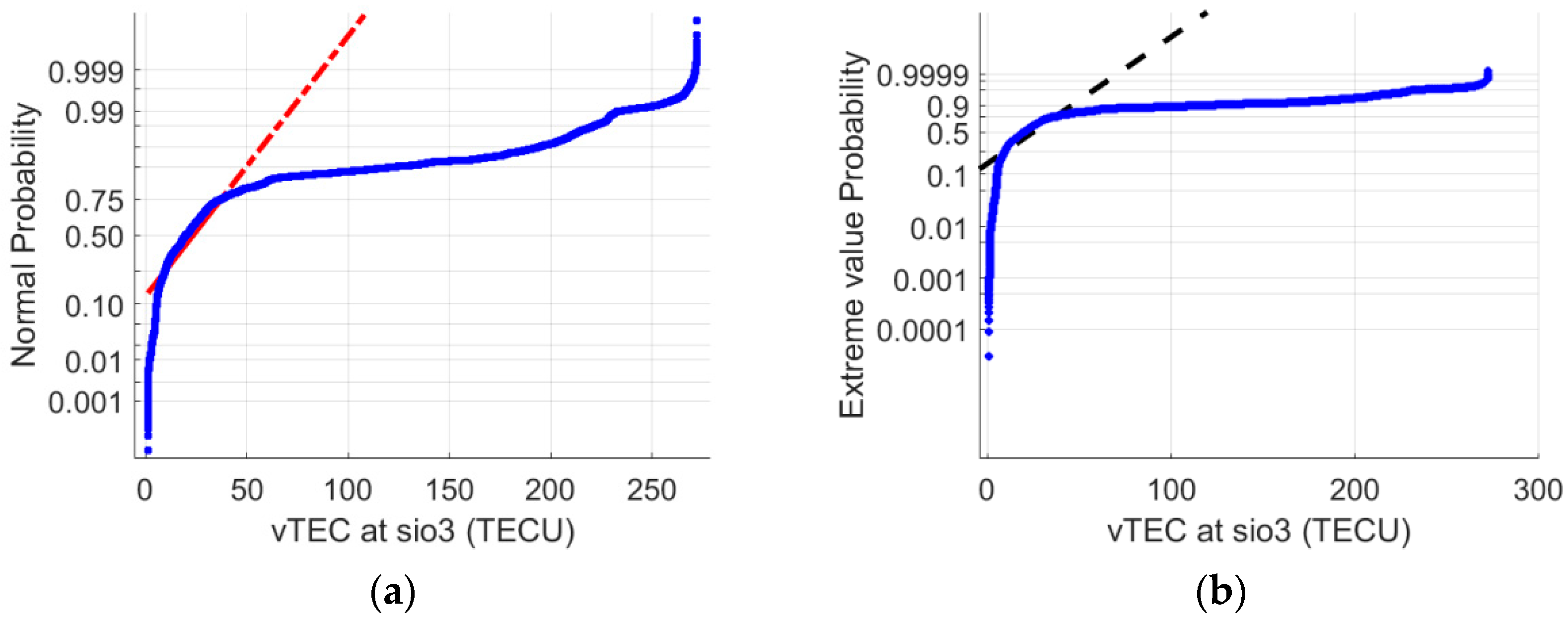
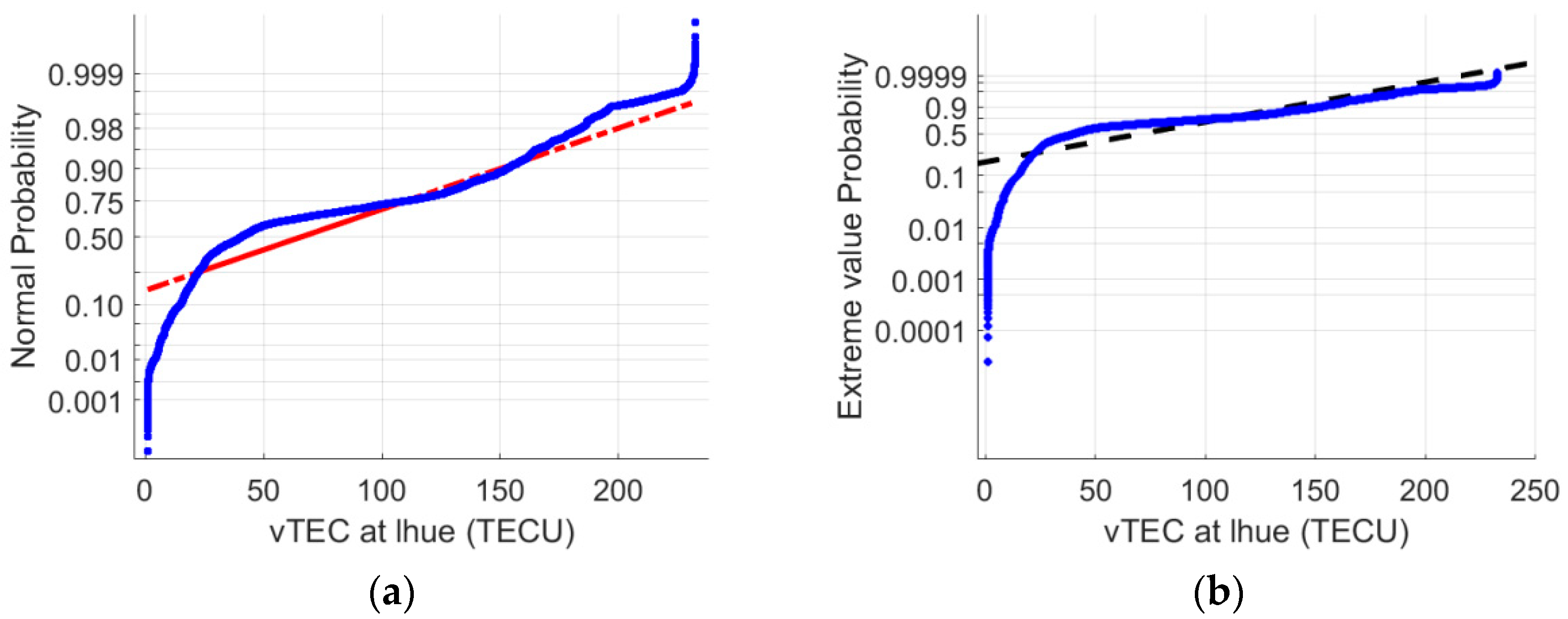
  • Define a maximum TEC value with an occurrence probability beyond 10−7 by exploratory data analysis (cf. [27]);
  • Define and adjust the overbounding model function and their parameter according to the data;
  • Perform a ray-tracing, to ensure that our approximations and the use of the ionospheric mapping function are not violating the conservatism of the approach.

2.4.2. Worst-Case Magnetic Induction

As apparent from (4), the geomagnetic induction is one of the impact parameters for second-order ionospheric effects. The International Geomagnetic Reference Field (IGRF) model 11th generation [28] is used to compute gridded maps of the geomagnetic induction at the Earth’s surface and at an ionospheric height of 350 km with 2.5 degree latitude and longitude resolution for an arbitrary date 1 January 2020. Analyzing these values, we found that the maximum geomagnetic induction is about 0.67 and 0.56 Gauss at the Earth’s surface and at an ionospheric height of 350 km, respectively. As a worst-case value for the geomagnetic induction, we choose 0.6 G, which reflects the strength of the geomagnetic field at ionospheric altitudes in the Polar Latitudes. Given that the magnetic induction is maximal in the Polar Regions, this value is seen as a representative upper bound for the global geomagnetic field strength.
To compute the overbounding model we make the following further assumptions:
  • The magnetic field is always constant (worst case) along the ray-path;
  • The azimuth is always set in a way that the magnetic induction is maximal (signal path parallel to magnetic field lines)

2.4.3. Linking Electron Density to TEC

As a first step to link the electron density to the TEC, we used the approximation of Brunner and Gu [4]:
  n e 2   d s = N m a x ·   η   n e   d s = N m a x ·   η   · T E C L o S .
Here, the integral of the squared electron density along the line of sight is replaced by the peak electron density Nmax, the total electron content along the line of sight (TECLoS), and a shape parameter η. The latter is set to 0.66 as an appropriate value to account for different electron density distributions [8,22].
Finally, to find an appropriate value for Nmax, we applied the model introduced by Pireaux et al., in 2010 [29]:
N m a x = ( 20 6 )   · 10 12 ( 4.55 1.38 )   · 10 18   · ( v T E C 4.55   · 10 18 ) + 20   · 10 12 .
The model links Nmax to the vertical TEC (VTEC). To complete the model to overbound the ionospheric-free residuals, the remaining task is to find extreme cases of TEC that fit the assumptions of the integrity risk.

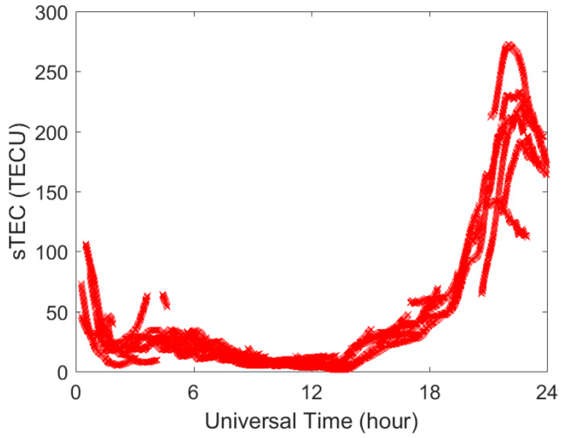
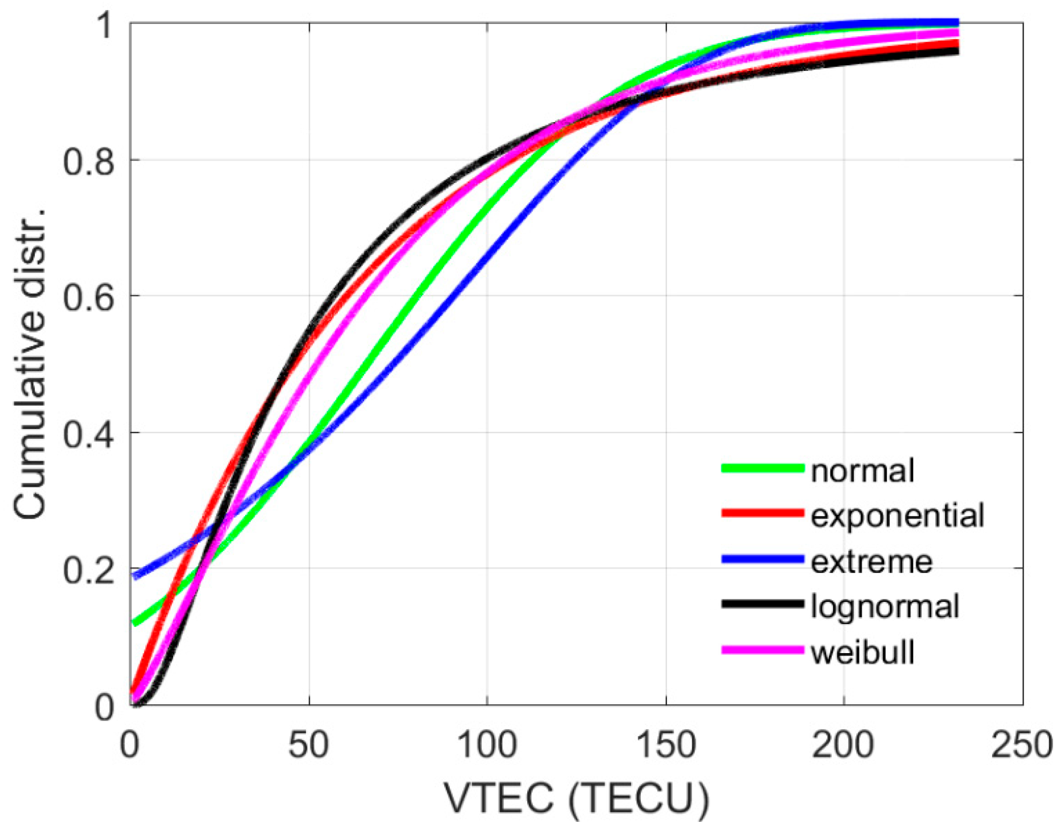
2.4.4. Selection of Extreme TEC Values

The first step to identify extreme TEC values is the analysis of the 42 most severe geomagnetic storm events that occurred since 1994 (selected by the geomagnetic indices Ap and kp), to identify dates and regions where the highest TEC values occurred. The TEC values and their associated locations are derived from post-processed daily 2-hourly CODE (Center for Orbit Determination Europe) TEC maps. The spatial resolution of these maps is 2.5° and 5° along latitude and longitude, respectively. A part of the outcome of this analysis is shown in Table 1. It lists the four dates and corresponding locations where the highest TEC values are found.
Taking into account that the CODE TEC maps are too smooth for an analysis of very extreme TEC events, we decided to not use the TEC values directly from this analysis. Only the dates and regions are used to preselect four IGS stations close to the regions where the highest CODE TEC values occurred. The selected stations are LHUE (Lihue, Kauai, HI, USA), HNLC (Honolulu, HI, USA), AMC2 (Colorado Springs, CO, USA), GOLD (Goldstone, CA, USA), and SIO3 (La Jolla, CA, USA).
For these stations, we processed the TEC from the GPS observations for the complete days with a time resolution of 30 s. An example of the output of this process is depicted in Figure 1. It shows the TEC variation derived for all GPS satellites visible at the IGS (International GNSS Service) station SIO3 versus universal time (UT) for 30 October 2003.
The maximum TEC values that we found for the 5 stations for 29 October 2003 and 30 October 2003 through this procedure are listed in Table 2.
Given the fact that the highest TEC values occurred on 30 October 2003 at the stations LHUE, HNLC, and SIO3, we further limited our analysis of the data of these three stations on only this date.
To derive a TEC value that represents a probability beyond 10−7 from this data, we looked for an appropriate statistical prediction model. First, we crosschecked the data against the following probability distributions: Normal, Exponential, Extreme value, Lognormal, and Weibull. Examples of the outcomes of this analysis for the Normal and Extreme value distributions are displayed in Figure 2, Figure 3 and Figure 4. We created a normal probability plot (e.g., Figure 2a) comparing the distribution of the data to the normal distribution. The broken reference line indicates whether the data follows a normal distribution or not. If the data points appear along the reference line, it confirms that the sample data has a normal distribution (see Figure 3a). If the distribution is not normal, it will introduce curvature in the data plot (see Figure 2a). Similarly, we created an extreme value probability plot (e.g., Figure 2b) comparing the distribution of the data to the extreme value distribution, and the broken reference line indicates whether the data follows an extreme value distribution or not. We used MATLAB built-in functions for obtaining probability distribution [30].
In a second step, we calculated the TEC from the inverse of the cumulative density function (CDF) of our model distributions. The corresponding cumulative distribution functions are given in Figure 5, and the final results of this procedure are depicted in Table 3. The latter lists the maximum TEC values obtained from the inverse CDF for a probability bound of 10−7.
Only after comparing the maximum TEC values observed (first column of Table 3) to the extrapolated TEC values for a probability bound of 10−7 obtained from inverse CDF analysis, we found that the Normal and Extreme Value distributions show acceptable results, whereas the Exponential, Lognormal, and Weibull distributions give TEC values far beyond any physical explanation. Since the probability distribution tests of the station SIO3 show a bad fitting performance of the models for the Normal and Extreme Value distributions (Figure 2, top and panels), we took the data from SIO3 out of our further considerations. The tests for the stations LHUE and HNLC show a reasonable fitting performance for both Normal and Extreme Value Distribution, as shown in Figure 3 and Figure 4. To conclude the selection process, we decided to take the higher of the two remaining values. Therefore, 354.0 TECU obtained from HNLC is the selected reference, and we determined 360 TECU as the maximum TEC to design our overbounding model. Obviously, this estimation has not led to a precise TEC estimate, but to an overestimated TEC as required for the overbounding model.

2.5. The Overbounding Model

To compute the overbounding model, one has to sum all residuals of the ionospheric-free combination for the worst-case conditions as described in the previous sections. In our approach, we use (8)–(10) with a maximum TEC value of 360 TECU, the mapping function as described in RTCA/DO-229D, a constant magnetic induction of 0.6 G, which is obtained at the magnetic poles, and an elevation range from 2 to 90 degrees. The choice of 0.6 G for all latitudes has the advantage that it will put additional margin (in terms of increasing the overbound) to lower latitudes, where the magnetic induction is lower. The results of the computations are depicted in Figure 6. It shows the elevation-dependent curves for the sum of all residuals, the sum of second- and third-order effects, the excess path, excess TEC, and the final overbounding model.
The final model (see Figure 7) is obtained by dividing the sum of all residuals by a factor of 5.33 to convert the standard deviation for the 10−7 probability to a one σ standard deviation and to fit a selected function that fulfills the requirement to be easy implementable in GNSS receiver software. This approach leads to the following overbounding model for the variance of the ionospheric-free residuals.
“When applying the ionospheric-free dual-frequency L1/L5 combination, the residual error (including ionospheric higher-order effects, ray bending, and excess TEC) in units of meters is described by the normal distribution Ɲ(0, σ2i,UIRE), where:
σ i ,   U I R E = 40.0 261.0 + ( E l i , d e g ) 2 + 0.018  
and Eli is elevation angle in degrees for the ith satellite. The model is valid down to an elevation angle of 3 degrees.”

3. Results

3.1. Model Justification by Ray-Tracing

As a final step for the justification of the model, we applied a ray-tracing technique. This method validates that the used approximations in computing different higher-order residuals and imprecisions introduced by the use of the mapping function do not lead to a violation of the conservativeness of the model. The approach is based on a two-dimensional ray-tracing technique developed by Hoque and Jakowski [12]. The anisotropy of the ionosphere, i.e., the effect of the Earth’s magnetic field on the signal propagation, has been taken into account. For this, the International Geomagnetic Reference Field (IGRF, [28]) model is applied when calculating geomagnetic field vectors at numerous points along incoming ray paths. The interactions among the signal, ionospheric electron density, and geomagnetic field lines are approximated by the Appleton–Hartree formula [31]. The ionosphere is assumed to be composed of numerous thin spherical layers in each of which the medium is homogeneous.

3.1.1. Modeling of the Earth’s Ionosphere and Plasmasphere

The electron density distribution of the Earth’s ionosphere is modeled by adding multiple Chapman layers superposed by an exponential decay function representing the plasmasphere. The Chapman layer [32] describes the electron density Ne distribution as a function of height (h) by
N e ( h ) = N e I ( h ) + N e P ( h ) ,
N e I ( h ) = N 0 e x p ( 0.5 ( 1 z s e c χ e x p ( z ) ) ) .
N e P ( h )     n p e x p ( h H P )   f o r   h     h m   &   0   f o r   h < h m ,
z = h h 0 H
where N e I ( h ) is the ionospheric electron density and N e P ( h ) is the plasmaspheric electron density, χ is the sun’s zenith angle, N0 is the peak electron density observed at the altitude h0 at zenith (χ = 0), and H is the atmospheric scale height. It can be shown that the maximum ionization N m =   N 0 c o s χ occurs at the height h m =   h 0 + H l n ( s e c χ ) [21]. The plasmaspheric density N e P ( h ) is modeled by an exponentially decreasing function of height where np is the plasmaspheric basic density of electrons and HP (10,000 km) is the mean scale height of the plasma density [33]. The plasmaspheric density contribution below the peak density height hm is set to zero.
The atmospheric scale height H, peak density Nm, and peak height hm practically define the shape of the Chapman layer; thus, by tuning these parameters, we can generate numerous electron density profiles with varying shapes. The expression for vertical TEC can be derived by integrating Equation (14) with respect to the height and written as [11]
V T E C I =   n e I ( h ) 4.13 H N m .
In order to simulate a broader variety of profile shapes, we superposed three Chapman layers representing the ionospheric E, F1, and F2 layers. The values of shape parameters H, Nm, and hm used for individual layers are determined by extensive literature research (e.g., [21,34,35,36,37,38,39]). We found that they could vary largely depending on geophysical conditions, which again depend on geographic/geomagnetic location as well as diurnal, seasonal, and solar cycle variation. Based on literature study, we set separate ranges for peak electron density heights hmF2, hmF1, hmE, and scale heights HF2, HF1, and HE of ionospheric F2, F1, and E layers as follows:
250   h m F 2   550   km ,    60   H F 2   90   km  
180   h m F 1   220   km ,    40   H F 1   60   km  
100   h m E   120   km ,    5   H E   15   km
Knowing the scale height and TEC contribution of the F2, F1, and E layers, the corresponding peak electron densities NmF2, NmF1, and NmE can be determined using Equation (16) by
N m F 2 = V T E C F 2 / ( 4.13 H F 2 )
N m F 1 = V T E C F 1 / ( 4.13 H F 1 )
N m E = V T E C E / ( 4.13 H E )
where VTECF2, VTECF1, and VTECE are the VTEC contributions from individual layers. The absolute maximum VTEC is determined as 360 TECU in a previous section. In order to describe a broader variety of geophysical conditions, we assume that about 5–20% (randomly fixed) of the ionospheric electron contribution comes from the F1 layer, about 0–5% (randomly fixed) comes from the E layer, and the rest of the electron contribution comes from the F2 layer (for more details, see Kelley [35] and Norman [37]). The solar zenith angle χ is varied within the range 0–80° when modeling each layer, and values above 80° are ignored to avoid complexity in the ionospheric model (Davies [36]). We further assumed that the plasmaspheric contribution could vary from about 5% to 10% (randomly fixed) of the total contribution.

3.1.2. Justification of Mapping Function

The ray-tracing results are used to verify the accuracy of the ionospheric mapping function. The ionospheric mapping function (MF) is used for vertical to slant TEC conversion and vice versa. There are several standards for the mapping function depending on the application (Figure 8). Here, we compare the MF recommended in MOPS 229D (see RTCA Inc. 2008 419, 2008 [25]), GPS ICD (see GPS Joint Program Office 2004), and the modified single-layer model mapping (MSLM) given by Dach et al. [40] with ray-tracing results. The MF algorithms can be found in the given references.
Figure 8 (right panel) compares the slant TEC variation for different MFs with ray tracing results (green plots). The mapping function results are mainly elevation-dependent, whereas the ray-tracing results depend not only on elevation but also on profile shapes, especially at low elevation angles. We see that at low elevation angles MOPS 229D (red solid line) and GPS ICD (black dashed line), the results are closer to the ray-tracing results (green line) when ray tracing gives higher STEC values. However, the MSLM (blue solid line) gives better results when ray tracing shows smaller STEC values. With the increase of the elevation angle, each MF model shows better performance.

3.1.3. Higher-Order Effects Estimation

The GPS L1 and L5 signals are traced through about 2000 electron density profiles (see left image of Figure 7), and higher-order ionospheric propagation terms including ray path bending effects are computed for single-frequency and dual-frequency ionosphere free linear combination. Figure 9 shows the variation of the second- and third-order residual terms, excess path length due to geometric bending, and excess TEC variation with the elevation angle.
Our investigation shows that the higher the peak electron density value, the higher the ray path bending effects. Additionally, the geometric bending effects (both excess path length and excess TEC) significantly increase with the decrease of the peak density height. It is worth pointing out that the geometric bending effects reduce to zero at 90° elevation angle (Figure 10).
For the second-order term estimation, we used a receiver location at –70° N latitude and 120° E longitude with a receiver-to-satellite azimuth angle set to 1°. The second-order effect significantly varies with the user location and user-to-satellite azimuth angle at a certain elevation angle. For a GNSS user in the northern hemisphere, the magnitude of the second-order term is largest when the signal is received from a satellite in a southward direction. However, for a user in the southern hemisphere, the situation is reversed, e.g., the largest effect is observed when the signal is received from a satellite in a northward direction [12]. Therefore, the receiver location and azimuth angle are selected in such a way that we get the highest values for the second-order term estimation.
The large variations of ray-tracing results come from broader varieties of profile shapes. Apparently, the residuals due to ray path bending (both excess path length and excess TEC) are much higher than the second- and third-order residuals at low elevation angle (e.g., <15°). However, they decrease very rapidly with increasing elevation angle and disappear at zenith. Although the second- and third-order residuals are less than bending residuals at low elevation angles, they become larger than bending errors at higher elevation angles (>45°). The second-order residual does not reduce significantly with increasing elevation angle and therefore cannot be ignored even at zenith. Similarly, the third-order residual does not vanish at zenith. We found that the second- and third-order residuals are much less for ray-tracing computation compared to the values plotted in Figure 6 (blue dashed line), especially at low elevation angles.
Simulation studies (see Figure 10a–d) show that the slant TEC varies from 360 to 1190 TECU. The corresponding second-order phase delay varies from 111 to 180 mm and 46 to 75 mm for the GPS L5 and L1 signals, respectively, whereas the residual error for the combined L1–L5 signal varies from 71 to 115 mm. The third-order phase delay varies from 6 to 43 mm and 2 to 13 mm for the GPS L5 and L1 signals, respectively. The third-order residual error for the combined signal varies from 10 to 72 mm. The excess path error varies from 0 to 496 mm and 0 to 154 mm for the GPS L5 and L1 signals, respectively whereas the excess path error for the combined signal varies from 0 to 278 mm. The excess TEC error for the combined GPS L1–L5 signal varies from 0 to 555 mm (see red plot of Figure 10a).
Figure 6 shows the second- and third-order residuals obtained by approximation formulas. The reason for the high values is that we have assumed a radio wave propagation along the magnetic field line (e.g., Θ = 0), which gives excessive high values for the second-order residual for high TEC values at low elevation angles. The right panel of Figure 9 shows that the total dual-frequency residuals for the GPS L1–L5 combination can reach up to 1000 mm at very low elevation angles. The comparison between the developed overbounding model and the ray-tracing results shows that the 5.33σ model overbounds the raytracing results for elevation angles equal to or greater than 3 degrees.

4. Conclusions

We presented a model to overbound ionospheric residuals that remain after the application of the ionospheric-free linear combination. The model is designed to fit the needs of the MOPS for the next generation of dual-frequency SBAS using Galileo [19]. The final model (defined by Equation (12) and depicted in Figure 7) is elevation-dependent, easy implementable in the receiver software, and provides a conservative estimate of the worse-case residuals with a risk probability beyond 10−7. The design of the model is based on worst-case estimates of the geomagnetic induction and TEC. The latter has been derived through the analysis of a number of geomagnetic storm events and exploratory analysis of TEC data that have been observed during the events. Finally, since a number of approximations (e.g., the mapping function, estimates of the peak electron density) have been used, our model has been validated by ray-tracing results.
Finally, it should be mentioned that the presented model has been approved by members of the EUROCAE (European Organization for Civil Aviation Equipment) and is included in the new Galileo MOPS for Satellite-Based Augmentation System Airborne Equipment [18]. Future activities will aim to provide a less conservative model that may give more margins in the integrity estimation e.g., for more demanding operations than LPV 200 or CAT I autoland.

Author Contributions

Both authors, S.S. and M.M.H., equally contributed to the developing of this manuscript. All authors have read and agreed to the published version of the manuscript.

Funding

The work presented was performed in the frame of European Space Agency (ESA) Purchase Order N. 5401002930 (Assumptions on Ionospheric Residuals, AIR). Part of the work was supported by the Initiative and Networking Fund of the Helmholtz-Gemeinschaft Deutscher Forschungszentren e.V. under grant numbers ZT-0007 (ADVANTAGE, Advanced Technologies for Navigation and Geodesy).

Conflicts of Interest

The authors declare no conflict of interest.

References

  1. Juan, J.M.; Sanz, S.; González-Casado, G.; Rovira-Garcia, A.; Camps, A.; Riba, J.; Barbosa, J.; Blanch, E.; Altadill, D.; Orus, R. Feasibility of precise navigation in high and low latitude regions under scintillation conditions. J. Space Weather Space Clim. 2018, 8. [Google Scholar] [CrossRef] [Green Version]
  2. Tiwari, R.; Strangeways, H.J. Regionally based alarm index to mitigate ionospheric scintillation effects for GNSS receivers. Space Weather 2015, 13, 72–85. [Google Scholar] [CrossRef] [Green Version]
  3. Demyanov, V.V.; Zhang, X.; Lu, X. Moderate Geomagnetic Storm Condition, WAAS Alerts and Real GPS Positioning Quality. J. Atmos. Sci. Res. 2019, 2. [Google Scholar] [CrossRef]
  4. Brunner, F.K.; Gu, M. An improved model for the dual frequency ionospheric correction of GPS observations. Manuscr. Geod. 1991, 16, 205–214. [Google Scholar]
  5. Bassiri, S.; Hajj, G.A. Higher-order ionospheric effects on the global positioning system observables and means of modelling them. Manuscr. Geod. 1993, 18, 280–289. [Google Scholar]
  6. Jakowski, N.; Porsch, F.; Mayer, G. Ionosphere-induced-ray-path bending effects in precise satellite positioning systems. Z. Für Satell. Position. Navig. Und Kommun. 1994, SPN 1/94, 6–13. [Google Scholar]
  7. Kedar, S.; Hajj, G.; Wilson, B.; Heflin, M. The effect of the second order GPS ionospheric correction on receiver positions. Geophys. Res. Lett. 2003, 30. [Google Scholar] [CrossRef]
  8. Fritsche, M.; Dietrich, R.; Knöfel, C.; Rülke, A.; Vey, S.; Rothacher, M.; Steigenberger, P. Impact of higher-order ionospheric terms on GPS estimates. Geophys. Res. Lett. 2005, 32. [Google Scholar] [CrossRef]
  9. Hernández-Pajares, M.; Juan, J.M.; Sanz, J.; Orús, R. Second-order ionospheric term in GPS: Implementation and impact on geodetic estimates. J. Geophys Res. 2007, 112, B08417. [Google Scholar] [CrossRef]
  10. Hoque, M.M.; Jakowski, N. Higher order ionospheric effects in precise GNSS positioning. J. Geod. 2006, 81, 259–268. [Google Scholar] [CrossRef]
  11. Hoque, M.M.; Jakowski, N. Mitigation of higher order ionospheric effects on GNSS users in Europe. GPS Solut. 2007, 12, 87–97. [Google Scholar] [CrossRef]
  12. Hoque, M.M.; Jakowski, N. Estimate of higher order ionospheric errors in GNSS positioning. Radio Sci. Am. Geophys. Union 2008, 43, RS5008. [Google Scholar] [CrossRef]
  13. Hoque, M.M.; Jakowski, N. New correction approaches for mitigating ionospheric higher order effects in GNSS applications. In Proceedings of the ION GNSS 2012, Institute of Navigation, Nashville, TN, USA, 17–21 September 2012; pp. 3444–3453. [Google Scholar]
  14. Hernández-Pajares, M.; Aragón-Ángel, À.; Defraigne, P.; Bergeot, N.; Prieto-Cerdeira, R.; Garcia-Rigo, A. Distribution and mitigation of higher-order ionospheric effects on precise GNSS processing. J. Geophys. Res. 2014, 119, 3823–3837. [Google Scholar] [CrossRef] [Green Version]
  15. Hadas, T.; Krypiak-Gregorczyk, A.; Hernández-Pajares, M.; Kaplon, J.; Paziewski, J.; Wielgosz, P.; Garcia-Rigo, A.; Kazmierski, K.; Sosnica, K.; Kwasniak, D.; et al. Impact and implementation of higher-order ionospheric effects on precise GNSS applications. J. Geophys. Res. Solid Earth 2017, 122. [Google Scholar] [CrossRef]
  16. Zhang, Z.; Guo, F.; Zhang, X. The Effects of Higher-Order Ionospheric Terms on GPS Tropospheric Delay and Gradient Estimates. Remote Sens. 2018, 10, 1561. [Google Scholar] [CrossRef] [Green Version]
  17. Cai, C.; Liu, G.; Yi, Z.; Cui, X.; Kuang, C. Effect analysis of higher-order ionospheric corrections on quad-constellation GNSS PPP. Meas. Sci. Technol. 2019, 30. [Google Scholar] [CrossRef]
  18. EUROCAE ED-259. Minimum Operational Performance Standards for Galileo-Global Positioning System-Satellite-Based Augmentation System Airborne Equipment; EUROCAE: Saint-Denis, France.
  19. ICAO. SBAS Safety Assessment Guidance Related to Anomalous Ionospheric Conditions; Adopted by APANPIRG/27; ICAO: Montreal, QC, Canada, 2016; EUROCAE: Saint-Denis, France, 2019. [Google Scholar]
  20. Taleb, N.N. The Black Swan: The Impact of the Highly Improbable; Random House: New York, NY, USA, 2007. [Google Scholar]
  21. Budden, K.G. The Propagation of Radio Waves: The Theory of Radio Waves of Low Power in the Ionosphere and Magnetosphere; Cambridge University Press: Cambridge, UK, 1985. [Google Scholar]
  22. Hartmann, G.; Leitinger, R. Range errors due to ionospheric and tropospheric effects for signal frequencies above 100MHz. Bull. Géodésique 1984, 58, 109–136. [Google Scholar] [CrossRef]
  23. Hoque, M.M. Higher Order Ionospheric Propagation Effects and Their Corrections in Precise GNSS positioning. Ph.D. Thesis, Universität Siegen, Siegen, Germany, 2009. [Google Scholar]
  24. Datta-Barua, S.; Walter, T.; Blanch, J.; Enge, P. Bounding higher-order ionosphere errors for the dual-frequency GPS user. Radio Sci. 2008, 43, RS5010. [Google Scholar] [CrossRef] [Green Version]
  25. RTCA Inc. 2008 419 Minimum Operational Performance Standard for Global Positioning System Wide Area Augmentation System Airborne Equipment; RTCA/DO-229D; RTCA Inc: Washington, DC, USA, 2008. [Google Scholar]
  26. Walter, T.; Enge, P.K.; Hansen, A.J. A Proposed Integrity Equation for WAAS MOPS. In Proceedings of the ION GPS 1997, Institute of Navigation, Kansas City, MO, USA, 16–19 September 1997; pp. 475–484. [Google Scholar]
  27. Downey, A.B. Think Stats: Exploratory Data Analysis; O’Reilly Media Inc.: Sebastopol, CA, USA, 2014. [Google Scholar]
  28. International Association of Geomagnetism and Aeronomy, Working Group V-MOD. International Geomagnetic Reference Field: The eleventh generation. Geophys. J. Int. 2010, 183, 1216–1230. [Google Scholar] [CrossRef] [Green Version]
  29. Pireaux, S.; Defraigne, P.; Wauters, L.; Bergeot, N.; Baire, Q.; Bruyninx, C. Higher-order ionospheric effects in GPS time and frequency transfer. GPS Solut. 2010, 14, 267–277. [Google Scholar] [CrossRef]
  30. Evans, M.; Hastings, N.; Peacock, B. Statistical Distributions, 2nd ed.; John Wiley & Sons, Inc.: Hoboken, NJ, USA, 1993. [Google Scholar]
  31. Appleton, E.V. Wireless studies of the ionosphere. J. Inst. Elec. Eng. 1932, 71, 642–650. [Google Scholar]
  32. Rishbeth, H.; Garriott, O.K. Introduction to Ionospheric Physics; Academic Press: New York, NY, USA, 1969. [Google Scholar]
  33. Jakowski, N.; Wehrenpfennig, A.; Heise, S.; Reigber, C.; Lühr, H.; Grunwaldt, L.; Meehan, T.K. GPS radio occultation measurements of the ionosphere from CHAMP: Early results. Geophys. Res. Lett. 2002, 29, 1457. [Google Scholar] [CrossRef] [Green Version]
  34. Decker, R.P. Techniques for synthesizing median true height profiles from propagation parameters. J. Atmos. Terr. Phys. 1972, 34, 451–464. [Google Scholar] [CrossRef]
  35. Kelley, M.C. The Earth’s Ionosphere, Plasmaphysics and Electrodynamics; Academic Press: New York, NY, USA, 1989. [Google Scholar]
  36. Davies, K. Ionospheric Radio; Peter Peregrinus Ltd.: London, UK, 1990; ISBN 086341186X. [Google Scholar]
  37. Norman, R.J. An Inversion Technique for obtaining Quasi-Parabolic layer parameters from VI Ionograms. In Proceedings of the 2003 Proceedings of the International Conference on Radar (IEEE Cat. No.03EX695), Adelaide, Australia, 3–5 September 2003; pp. 363–367. [Google Scholar] [CrossRef]
  38. Stankov, S.M.; Jakowski, N. Topside ionospheric scale height analysis and modeling based on radio occultation measurements. J. Atmos. Sol. Terr. Phys. 2006, 68, 134–162. [Google Scholar] [CrossRef]
  39. Jakowski, N.; Leitinger, R.; Angling, M. Radio occultation techniques for probing the ionosphere. Ann. Geophys. 2004, 47. [Google Scholar] [CrossRef]
  40. Dach, R.; Hugentobler, U.; Fridez, P.; Meindl, M. Bernese GPS Software Version 5.0. University of Bern. 2007. Available online: http://www.bernese.unibe.ch/docs50/DOCU50.pdf (accessed on 7 July 2020).
Figure 1. TEC variations versus universal time (UT), derived from measurements of the IGS station SIO3 (La Jolla, CA, USA) at 30 October 2003.
Remotesensing 12 02467 g001
Figure 2. Probability distribution tests of TEC against the Normal (panel a) and the Extreme Value (panel b) distributions. The TEC data are from the SIO3 station from 30 October 2003. Red and black broken lines represent normal and extreme value distribution, respectively.
Remotesensing 12 02467 g002
Figure 3. Probability distribution tests of TEC against the Normal (panel a) and the Extreme Value (panel b) distributions. The TEC data are from the LHUE station from 30 October 2003. Red and black broken lines represent normal and extreme value distribution, respectively.
Remotesensing 12 02467 g003
Figure 4. Probability distribution tests of TEC against the Normal (panel a) and the Extreme Value (panel b) distributions. The TEC data are from the station HNLC station from 30 October 2003. Red and black broken lines represent normal and extreme value distribution, respectively.
Remotesensing 12 02467 g004
Figure 5. Cumulative probability distributions (Normal, Exponential, Extreme value, Lognormal, Weibull) for vertical TEC from the station HNLC at 30 October 2003.
Remotesensing 12 02467 g005
Figure 6. The overbounding model and its components. Sum of all residuals (cyan), the sum of second- and third-order effects (blue), the excess path (green), excess TEC (black), and the overbounding model (red). The underlying assumptions developed in the upper sections of this paper are: maximum TEC of 360 TECU, magnetic induction of 0.6G, single layer height of 350 km.
Remotesensing 12 02467 g006
Figure 7. The final overbounding model.
Remotesensing 12 02467 g007
Figure 8. Left image (a) shows about 2000 simulated profiles for the same vertical TEC (VTEC) of 360 TECU. The right panel (b) shows the variation of slant TECs computed by different mapping functions (MFs) as well as by ray tracing (green plot) as a function of elevation angle.
Remotesensing 12 02467 g008
Figure 9. Top left (a) and top right (b) plots give ray-tracing estimates of second- and third-order group delay. Bottom left panel (c) shows geometric bending (i.e., excess path length) for GPS L1, L5, and combined L1–L5 signals whereas right panel (d) shows excess TEC in comparison with line of sight (LoS) TEC variation.
Remotesensing 12 02467 g009
Figure 10. Left panel (a) shows ray-tracing estimates of higher-order residuals in the GPS L1–L5 combination. The right panel (b) shows the total group delay residuals estimated by the overbounding model and corresponding ray-tracing results.
Remotesensing 12 02467 g010
Table 1. Preselected dates and locations showing maximum total electron count (TEC) in TEC Units (TECU).
DateApMax TEC/TECULat/°NLong /°E
29 October 2003204228.222.5−150.0
30 October 2003191216.527.5−130.0
7 April 200074178.020.0−160.0
31 March 2001192175.525.0115.0
Table 2. Maximum TEC observed at 29 October 2003 and 30 October 2003 at five selected stations. LHUE: Lihue, Kauai, HI, USA; HNLC: Honolulu, HI, USA; AMC2: Colorado Springs, CO, USA; GOLD: Goldstone, CA, USA.
StationLHUEHNLCAMC2GOLDSIO3
Max TEC/TECU at 29 October 2003212.5209.0194.3190.1182.6
Max TEC/TECU at 30 October 2003232.5232.3204.7201.7272.2
Table 3. Maximum TEC values, obtained from inverse cumulative density function (CDF) for a probability bound of 10−7 (derived from data of 3 IGS stations from 30 October 2003).
IGS
Station
Observed Max TEC (TECU)Extrapolated TEC/TECU
NormalExponentialExtremeLognormalWeibull
SIO3272.2329.0645.8293.66582.5899.4
LHUE232.5346.61046.3259.76208.9690.0
HNLC232.3354.01073.0263.96274.2701.9

