3D Fine-scale Terrain Variables from Underwater Photogrammetry: A New Approach to Benthic Microhabitat Modeling in a Circalittoral Rocky Shelf

 , ,
, , 
Abstract
1. Introduction
2. Materials and Methods
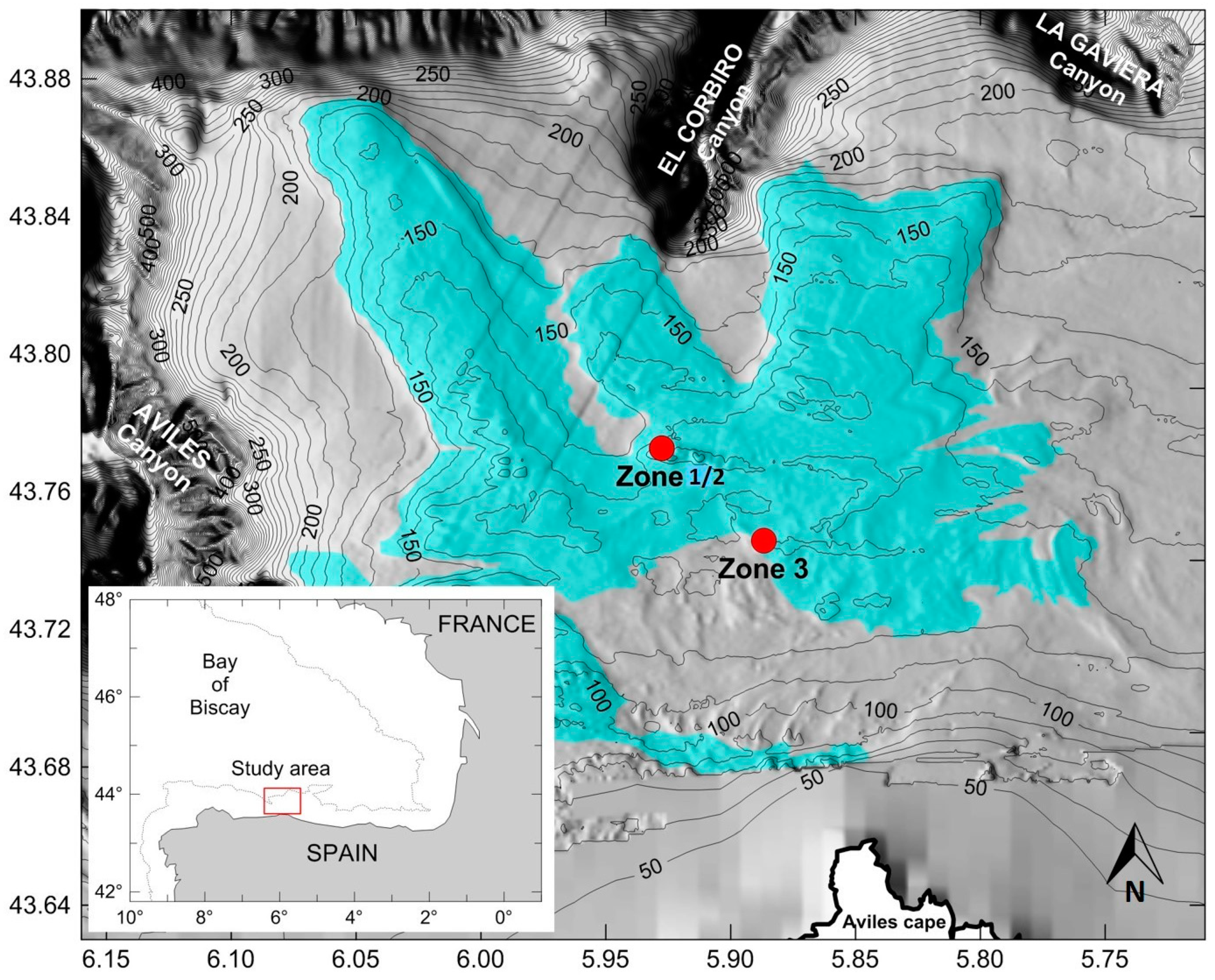
2.1. Study Area
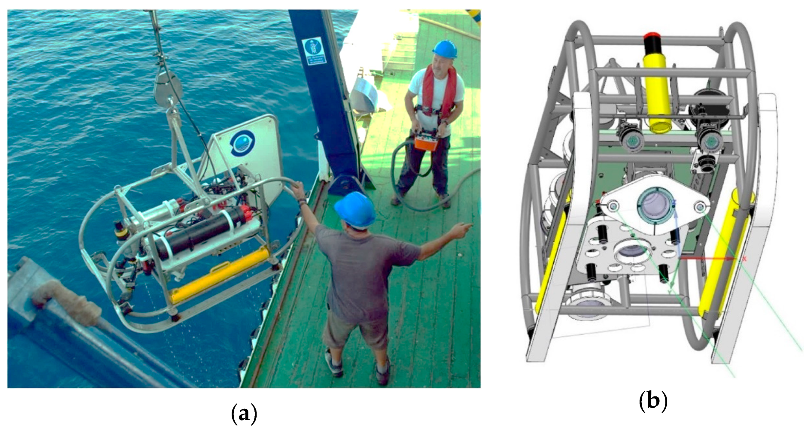
2.2. Survey Description and Image Acquisition
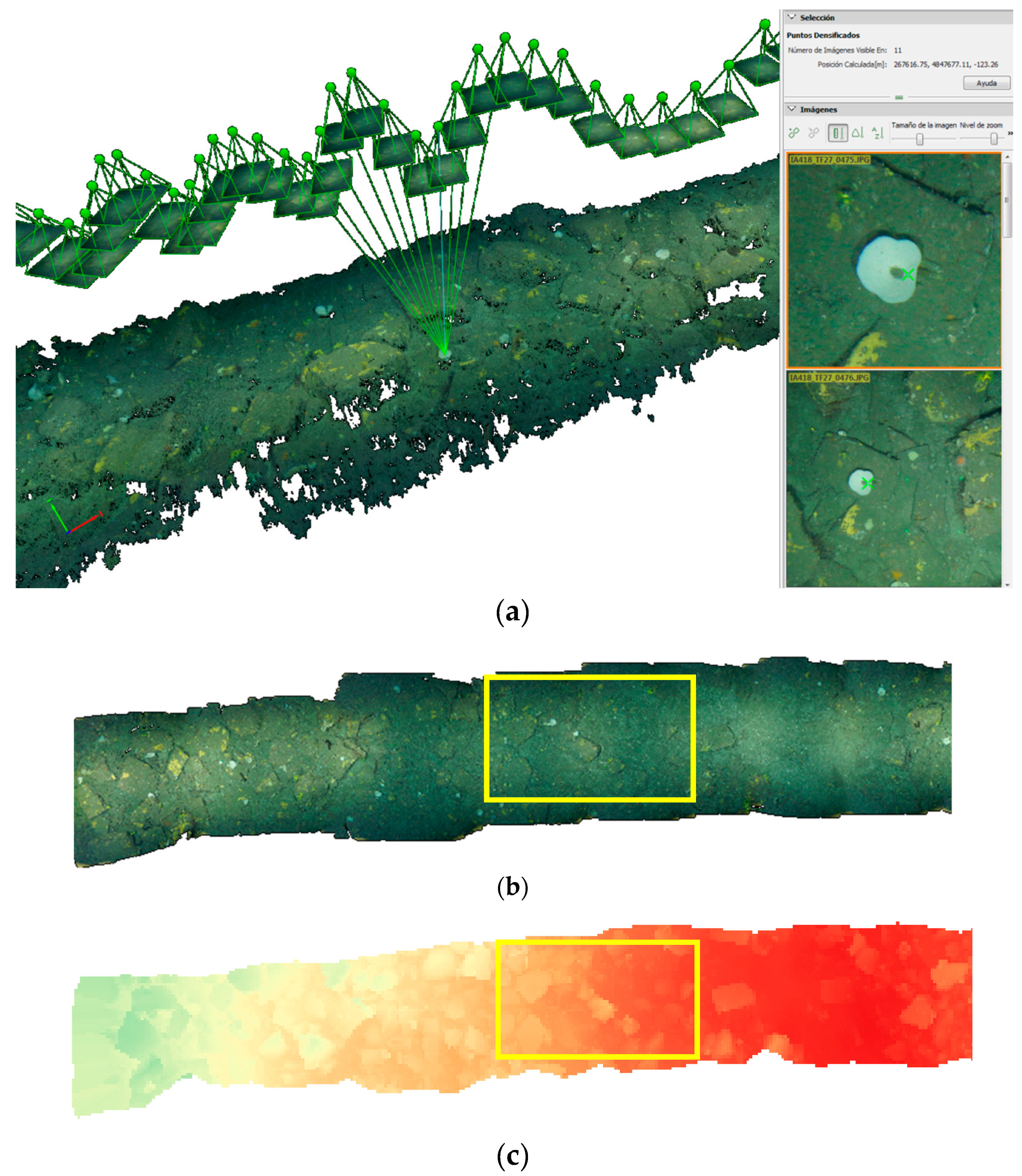
2.3. 3D Image Reconstruction and Digital Surface Model
2.4. Terrain Analysis
2.5. Faunal Presences
2.6. Significant Terrain Variables and Habitat Suitability Model
2.7. First Approximation of Automatic Image Annotation of Species Using Deep-Learning
3. Results
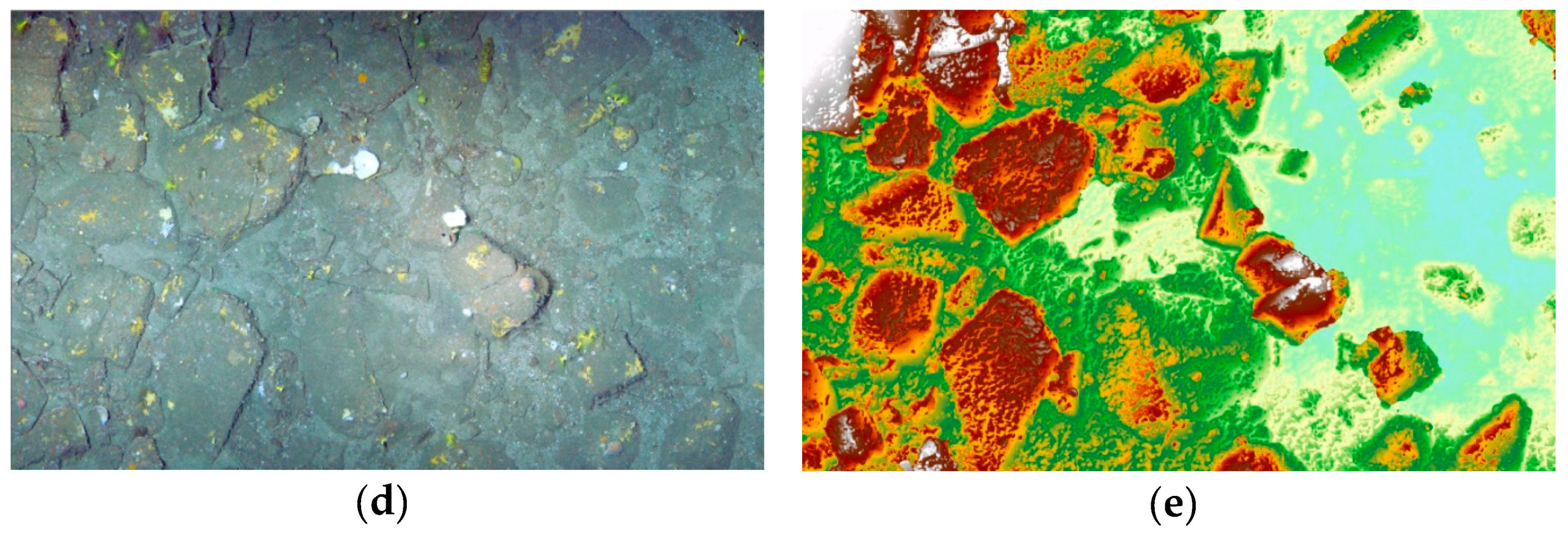
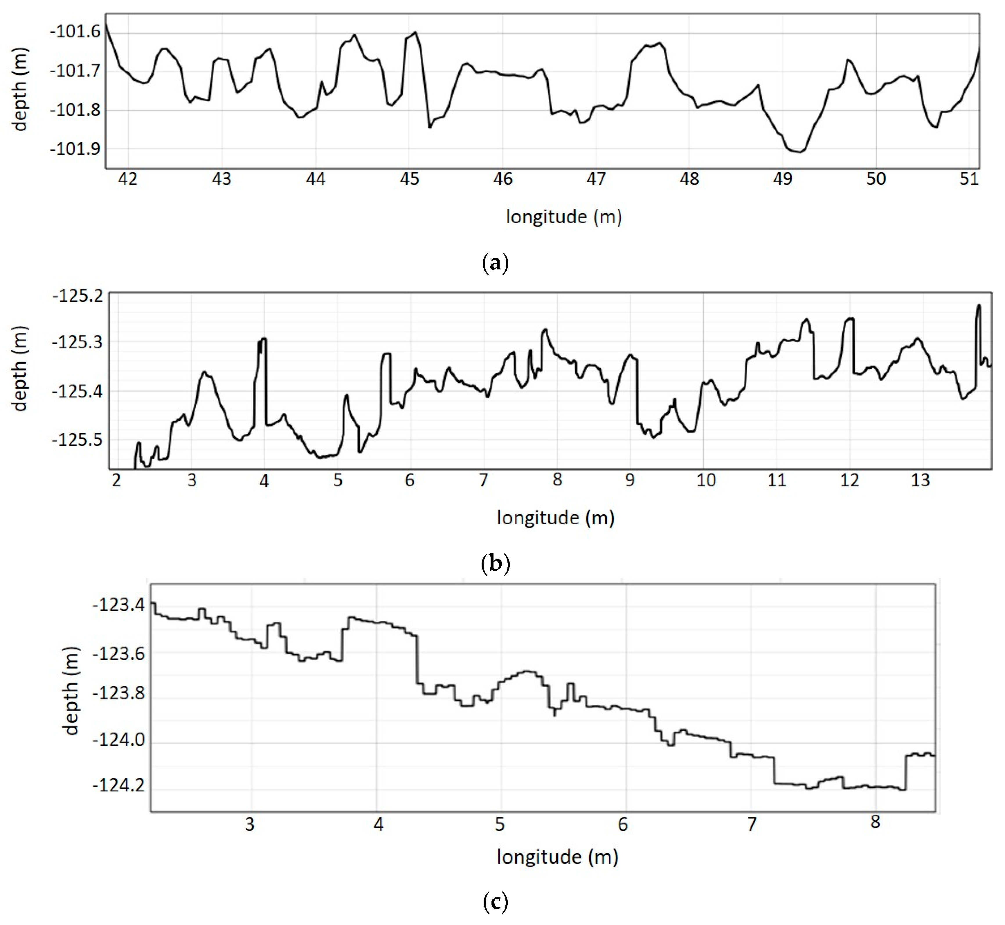
3.1. 3D Model, Digital Surface Model and Terrain Variables
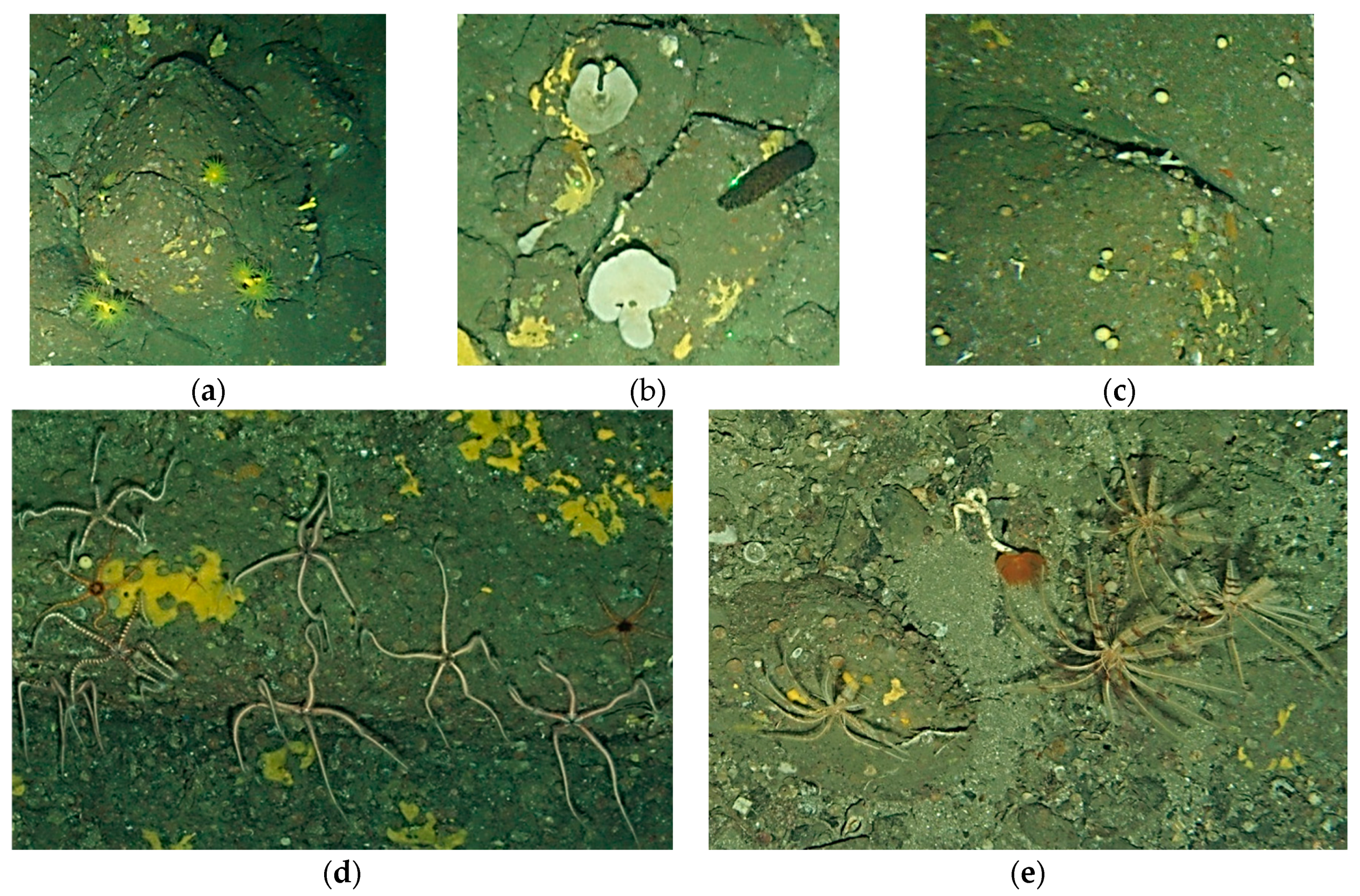
3.2. Environmental Characteristics of Studied Sites and Faunal Presence
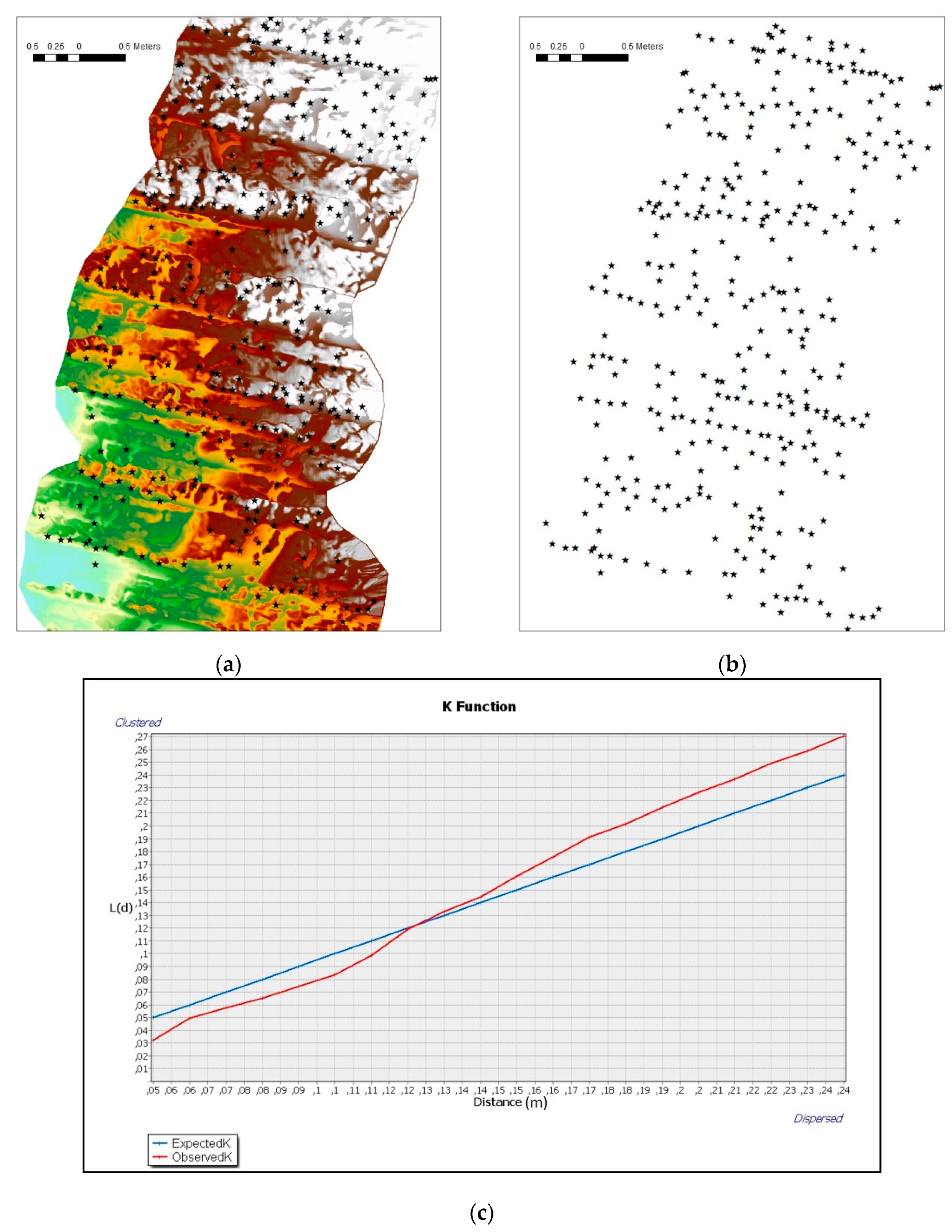
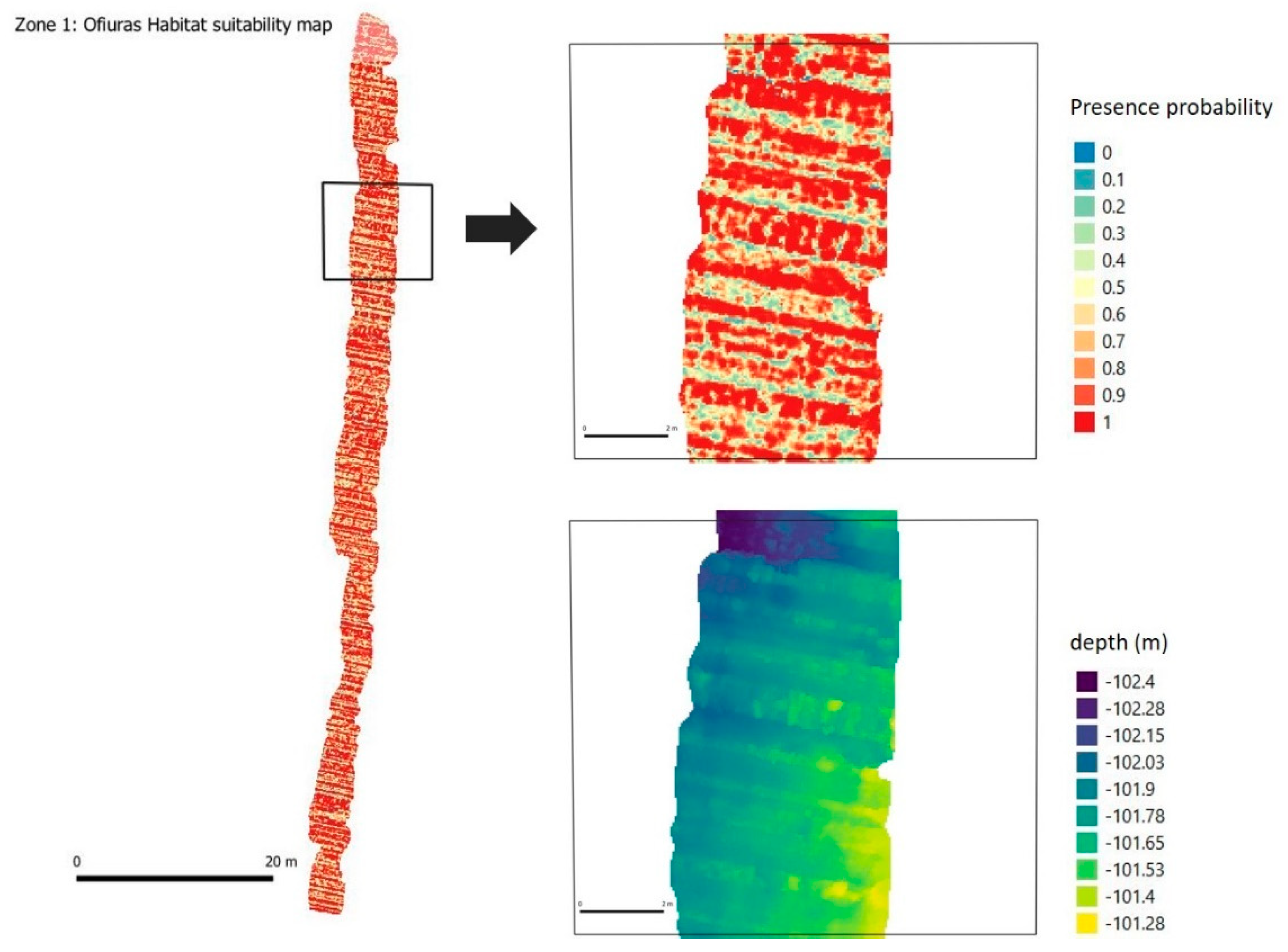
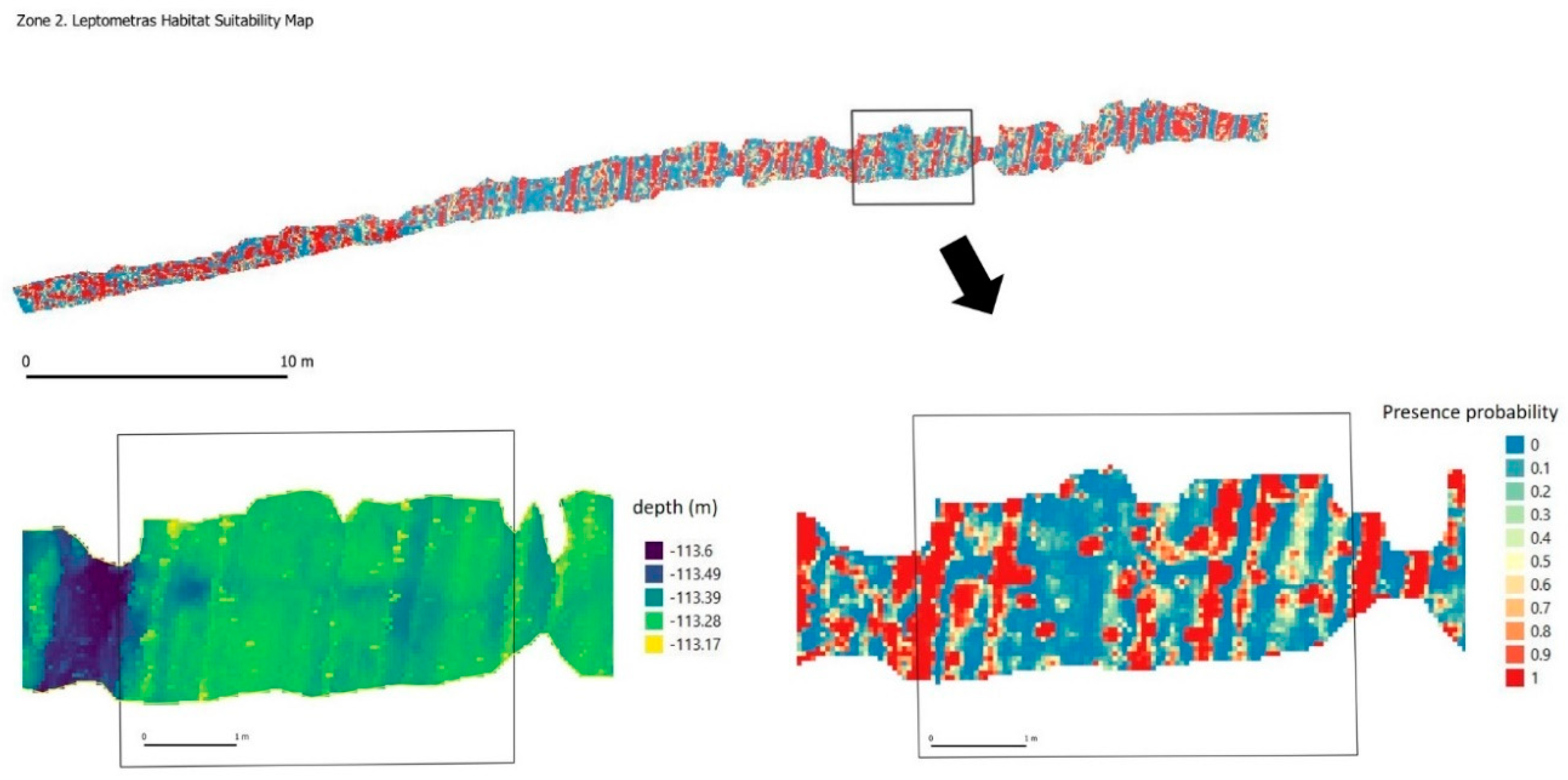
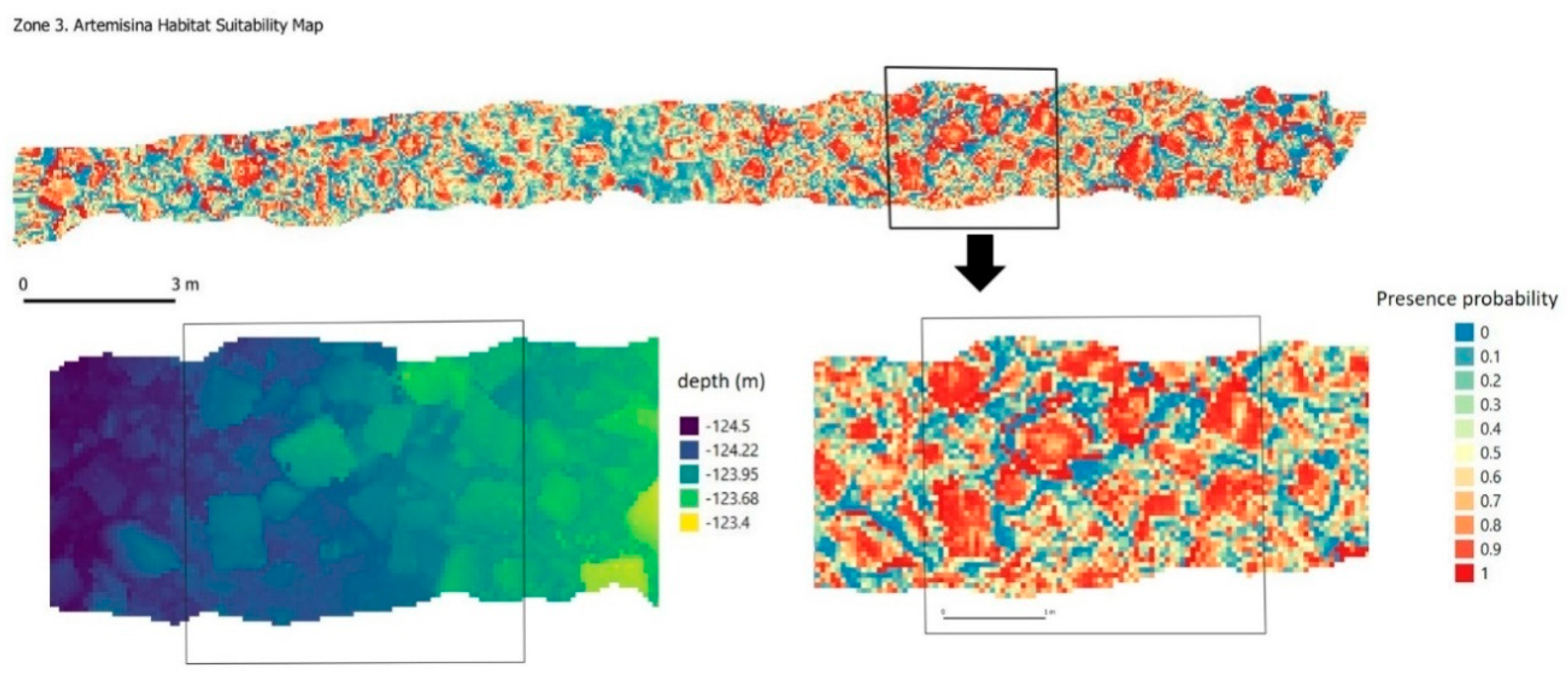
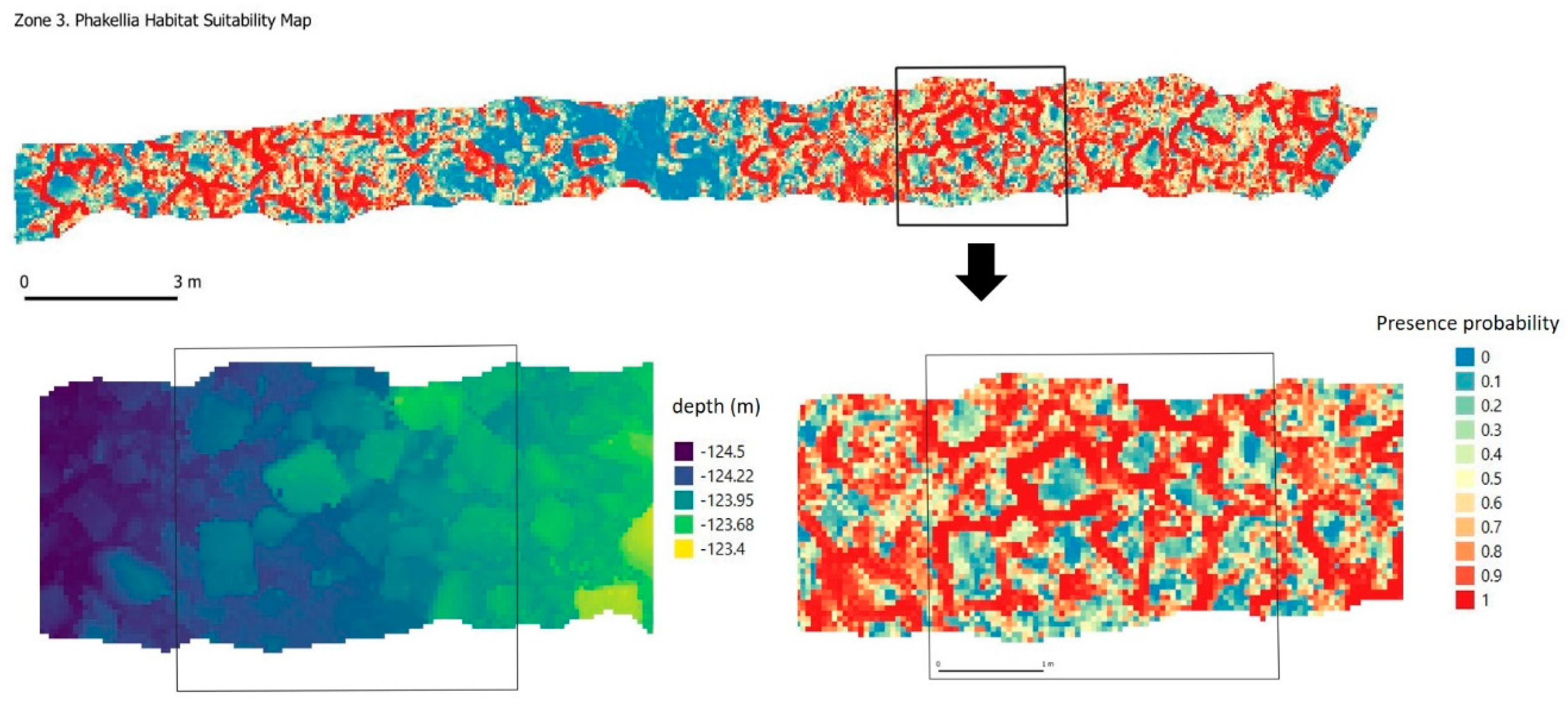
3.3. Significant Terrain Variables and Habitat Suitability Model
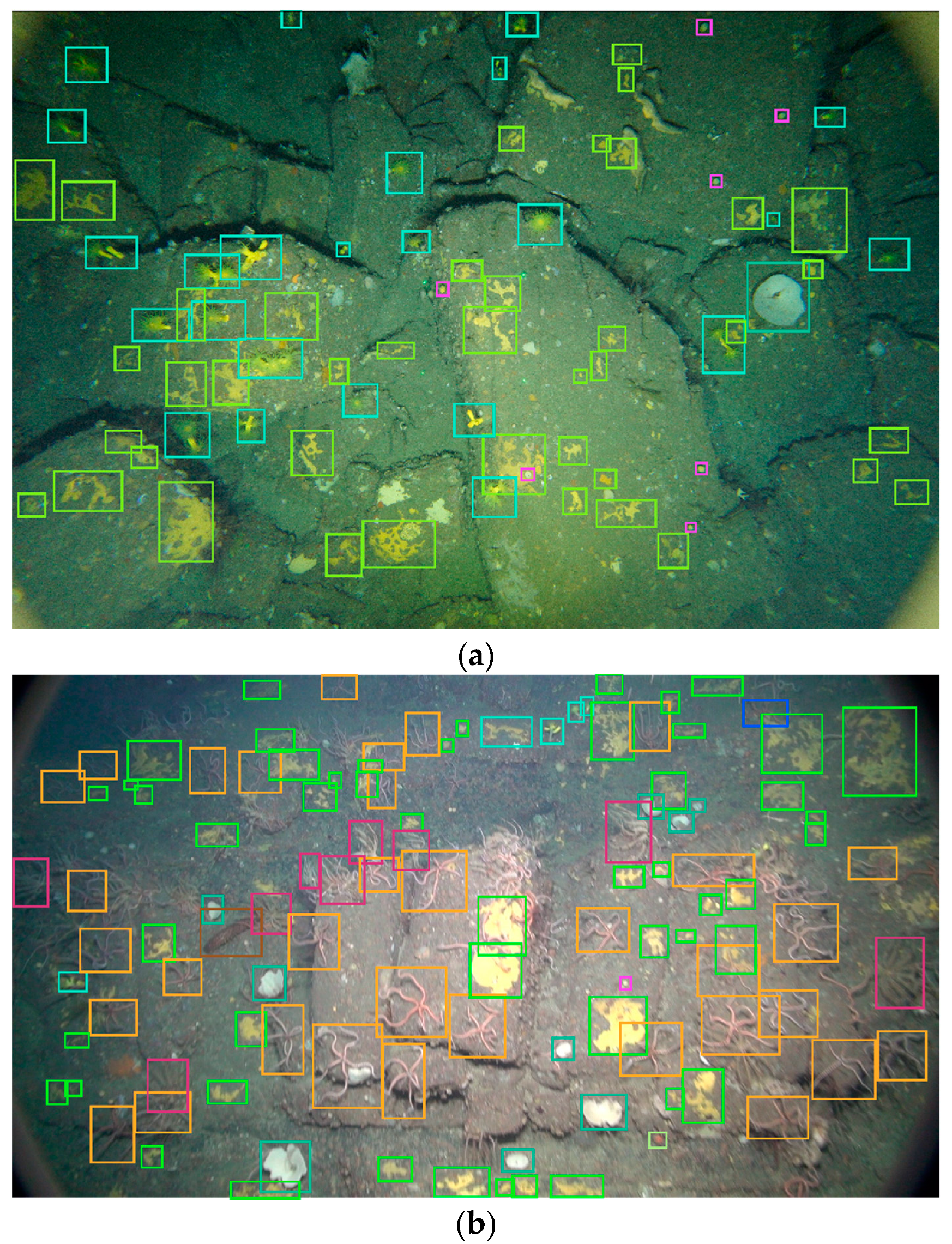
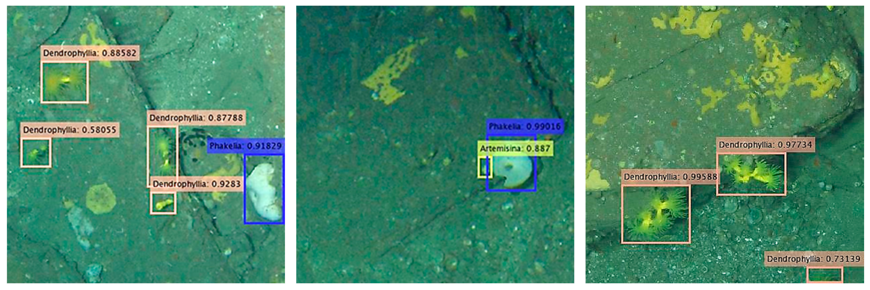
3.4. Automatic Presence Record Annotation
4. Discussion
4.1. 3D Photogrammetry to Improve Habitat Suitability Models
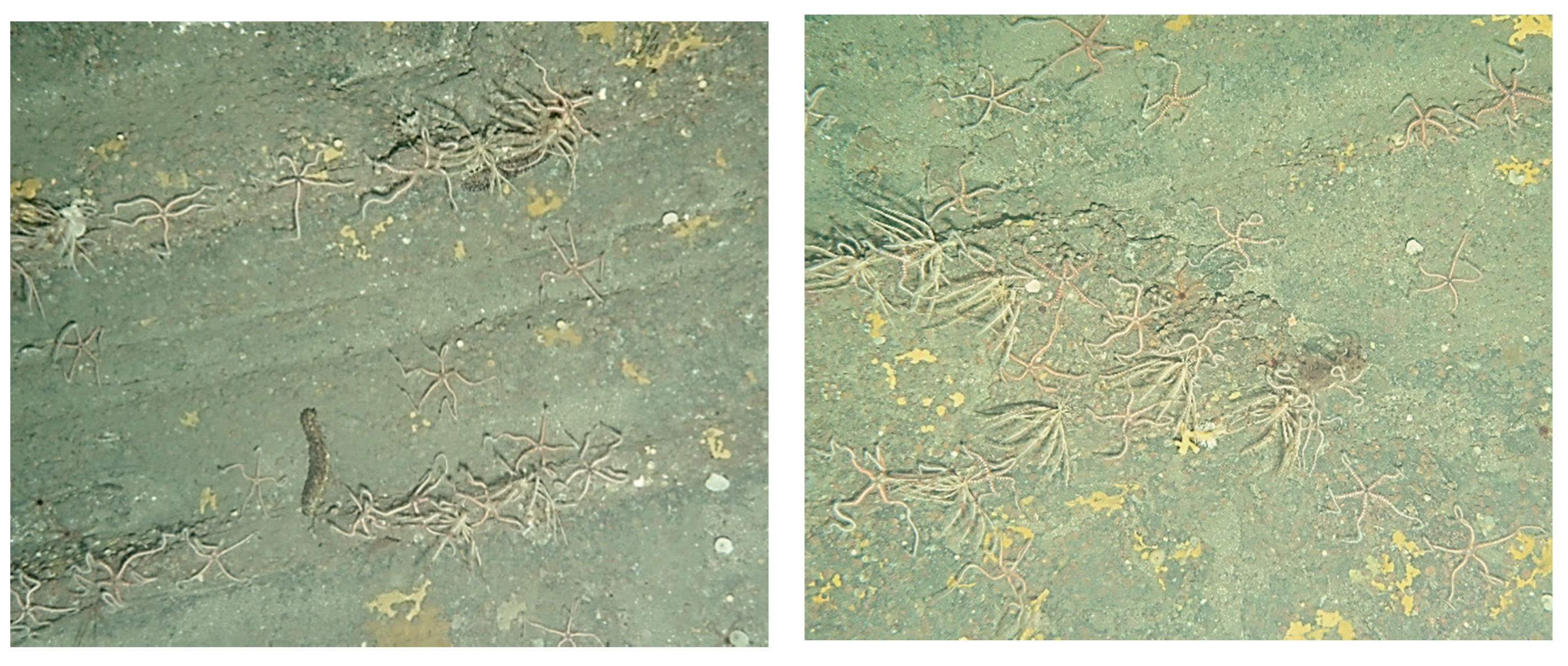
4.2. Spatial Distribution and Behavior of Species
4.3. Implementation of Deep-Learning Techniques to Annotate Benthic Species in Images
5. Conclusions
Author Contributions
Funding
Acknowledgments
Conflicts of Interest
References
- Council of Europe; Group of Experts on Protected Areas and Ecological Networks. Interpretation Manual of the Habitats Listed in Resolution No. 4 (1996). Listing Endangered Natural Habitats Requiring Specific Conservation Measures; Third Draft Version 2015; Council of Europe: Strasbourg, Franch, 31 August 2015; T-PVS/PA (2015) 9. [Google Scholar]
- Sánchez, F.; Rodríguez-Basalo, A.; Gómez-Ballesteros, M.; Prado, E.; Patrocinio, T.; Ríos, P.; Punzon, A.; Rueda, J.; Cristobo, J. Habitats characterization of circalittoral rocky bottoms of the Avilés Canyon System (Cantabrian Sea). Front. Mar. Sci. Conf. Abstr. XX Iber. Symp. Mar. Biol. Stud. (SIEBM XX) 2019. [Google Scholar] [CrossRef]
- Ríos, P.; Aguilar, R.; Torriente, A.; Muñoz, A.; Cristobo, J. Sponge grounds of Artemisina (Porifera, Demospongiae) in the Iberian Peninsula, ecological characterization by ROV techniques. Zootaxa 2018, 4466, 95–123. [Google Scholar] [CrossRef] [PubMed]
- Sánchez, F.; Serrano, A.; Ballesteros, M.G. Photogrammetric quantitative study of habitat and benthic communities of deep Cantabrian Sea hard grounds. Cont. Shelf Res. 2009, 29, 1174–1188. [Google Scholar] [CrossRef]
- Ross, R.E.; Howell, K.L. Use of predictive habitat modelling to assess the distribution and extent of the current protection of ‘listed’ deep-sea habitats. Divers. Distrib. 2013, 19, 433–445. [Google Scholar] [CrossRef]
- González-Mirelis, G.; Buhl-mortensen, P. Modelling benthic habitats and biotopes off the coast of Norway to support spatial management Ecological Informatics Modelling benthic habitats and biotopes off the coast of Norway to support spatial management. Ecol. Inform. 2015, 30, 284–292. [Google Scholar] [CrossRef]
- Sánchez, F.; Rodríguez-Basalo, A.; García-Alegre, A.; Gómez-Ballesteros, M. Hard-bottom bathyal habitats and keystone epibenthic species on Le Danois Bank (Cantabrian Sea). J. Sea Res. 2017, 130, 134–135. [Google Scholar] [CrossRef]
- Galparsoro, I.; Borja, Á.; Kostylev, V.E.; Rodríguez, J.G.; Pascual, M.; Muxika, I. Estuarine Coastal and Shelf Science A process-driven sedimentary habitat modelling approach, explaining sea floor integrity and biodiversity assessment within the European Marine Strategy Framework Directive. Estuar. Coast. Shelf Sci. 2013, 131, 194–205. [Google Scholar] [CrossRef]
- Zapata-Ramírez, P.A.; Huete-stauffer, C.; Scaradozzi, D.; Marconi, M.; Cerrano, C. Testing methods to support management decisions in coralligenous and cave environments. A case study at Porto Fino MPA. Mar. Environ. Res. 2016, 118, 45–56. [Google Scholar] [CrossRef]
- Buhl-Mortensen, L.; Buhl-Mortensen, P.; Dolan, M.J.F.; Gonzalez-Mirelis, G. Habitat mapping as a tool for conservation and sustainable use of marine resources: Some perspectives from the MAREANO Programme, Norway. J. Sea Res. 2015, 100, 46–61. [Google Scholar] [CrossRef]
- Fulton, E.; Bax, N.; Bustamante, R.; Dambacher, J.; Dichmont, C.; Dunstan, P.; Hayes, K.; Hobday, A.; Pitcher, C.; Plaganyi, E.; et al. Modelling marine protected areas: Insights and hurdles. Biol. Sci. 2015, 370, 20140278370. [Google Scholar] [CrossRef]
- Rodríguez-Basalo, A.; Sánchez, F.; Punzón, A.; Gómez-Ballesteros, M. Updating the Master Management Plan for El Cachucho MPA (Cantabrian Sea) using a spatial planning approach. Cont. Shelf Res. 2019, 184, 54–65. [Google Scholar] [CrossRef]
- Brown, C.J.; Smith, S.J.; Lawton, P.; Anderson, J.T. Estuarine, Coastal and Shelf Science Benthic habitat mapping: A review of progress towards improved understanding of the spatial ecology of the sea floor using acoustic techniques. Estuar. Coast. Shelf Sci. 2011, 92, 502–520. [Google Scholar] [CrossRef]
- Rowden, A.A.; Anderson, O.F.; Georgian, S.E.; Bowden, D.A.; Clark, M.R.; Pallentin, A.; Miller, A. High-Resolution Habitat Suitability Models for the Conservation and Management of Vulnerable Marine Ecosystems on the Louisville Seamount Chain, South Pacific Ocean. Front. Mar. Sci. 2017, 4, 335. [Google Scholar] [CrossRef]
- Guinotte, J.; Baco, A.; Black, J.; Hall-spencer, J.M. Global habitat suitability of cold-water octocorals. J. Biogeogr. 2012, 39, 1278–1292. [Google Scholar] [CrossRef]
- Lecours, V.; Devillers, R.; Schneider, D.C. Spatial scale and geographic context in benthic habitat mapping: Review and future directions. Mar. Ecol. Prog. Ser. 2015, 535, 259–284. [Google Scholar] [CrossRef]
- Greene, H.G.; Yoklavich, M.M.; Starr, R.M.; O’Connell, V.M.; Wakefield, W.W.; Sullivan, D.E.; McRea, J.E., Jr.; Cailliet, G.M. A classification scheme for deep seafloor habitats. Oceanol. Acta 1999, 22, 663–678. [Google Scholar] [CrossRef]
- Katya, K.; Sidinei, T.; Danielle, W. Habitat complexity: Approaches and future directions Habitat complexity: Approaches and future directions. Hydrobiologia 2012, 685. [Google Scholar] [CrossRef]
- Lingo, M.E.; Szedlmayer, S.T. The Influence of Habitat Complexity on Reef Fish Communities in the Northeastern Gulf of Mexico. Environ. Biol. Fishes 2006, 76, 71–80. [Google Scholar] [CrossRef]
- Moore, E.C.; Hovel, K.A. Relative influence of habitat complexity and proximity to patch edges on seagrass epifaunal communities. Oikos 2010, 119, 1299–1311. [Google Scholar] [CrossRef]
- Rees, M.J.; Knot, N.A.; Neilson, J.M.; Linklater, M.; Osterloh, I.; Jordan, A.; Davis, A.R. Accounting for habitat structural complexity improves the assessment of performance in no-take marine reserves. Biol. Conserv. 2018, 224, 100–110. [Google Scholar] [CrossRef]
- Gerovasileiou, V.; Chintiroglou, C.C.; Konstantinou, D. Sponges as ‘living hotels’ in Mediterranean marine caves. Sci. Mar. 2016, 80. [Google Scholar] [CrossRef]
- Kalacska, M.; Chmura, G.L.; Lucanus, O.; Bérubé, D.; Arroyo-Mora, J.P. Structure from motion will revolutionize analyses of tidal wetland landscapes. Remote Sens. Environ. 2017, 199, 14–24. [Google Scholar] [CrossRef]
- Palma, M.; Rivas-Casado, M.; Pantaleo, U.; Pavoni, G.; Pica, D.; Cerrano, C. SfM-Based Method to Assess Gorgonian Forests (Paramuricea clavata (Cnidaria, Octocorallia)). Remote Sens. 2018, 10, 1154. [Google Scholar] [CrossRef]
- Prado, E.; Sánchez, F.; Rodríguez-Basalo, A.; Altuna, Á.; Cobo, A. Analysis of the population structure of a gorgonian forest (Placogorgia sp.) using a photogrammetric 3D modeling approach at Le Danois Bank, Cantabrian Sea. Deep. Res. Part I Oceanogr. Res. Pap. 2019, 153. [Google Scholar] [CrossRef]
- Prado, E.; Sánchez, F.; Rodríguez-Basalo, A.; Altuna, Á.; Cobo, A. Semi-Automatic Method of Fan Surface Assessment to Achieve Gorgonian Population Structure in Le Danois Bank, Cantabrian Sea. ISPRS Int. Arch. Photogramm. Remote. Sens. Spat. Inf. Sci. 2019, XLII-2/W10, 2–3. [Google Scholar] [CrossRef]
- Bennecke, S.; Kwasnitschka, T.; Metaxas, A.; Dullo, W.C. In situ growth rates of deep-water octocorals determined from 3D photogrammetric reconstructions. Coral Reefs 2016, 35, 1227–1239. [Google Scholar] [CrossRef]
- Olinger, L.K.; Scott, A.R.; Mcmurray, S.E.; Pawlik, J.R. Growth estimates of Caribbean reef sponges on a shipwreck using 3D photogrammetry. Sci. Rep. 2019, 9, 18398. [Google Scholar] [CrossRef]
- Leon, J.X.; Roelfsema, C.M.; Saunders, M.I.; Phinn, S.R. Measuring coral reef terrain roughness using ‘Structure-from-Motion’ close-range photogrammetry. Geomorphology 2015, 242, 21–28. [Google Scholar] [CrossRef]
- Young, G.C.; Dey, S.; Rogers, A.D.; Exton, D. Correction: Cost and time-effective method for multi-scale measures of rugosity, fractal dimension, and vector dispersion from coral reef 3D models. PLoS ONE 2018, 13, e0201847. [Google Scholar] [CrossRef]
- He, H.; Ferrari, R.; McKinnon, D.; Roff, G.; Smith, R.; Mumby, P.; Upcroft, B.H. Measuring Reef Complexity and Rugosity from Monocular Video Bathymetric Measuring reef complexity and rugosity from monocular video bathymetric reconstruction. In Proceedings of the 12th International Coral Reef Symposium, Cairns, Australia, 9–13 July 2012; pp. 1–5. [Google Scholar]
- Ferrari, R.; McKinnon, D.; He, H.; Smith, R.N.; Corke, P.; González-Rivero, M.; Mumby, P.J.; Upcroft, B. Quantifying multiscale habitat structural complexity: A cost-effective framework for underwater 3D modelling. Remote Sens. 2016, 8, 113. [Google Scholar] [CrossRef]
- Price, D.M.; Robert, K.; Callaway, A.; lacono, C.L.; Hall, R.A.; Huvenne, V.A.I. Using 3D photogrammetry from ROV video to quantify cold- water coral reef structural complexity and investigate its influence on biodiversity and community assemblage. Coral Reefs 2019, 38, 1007–1021. [Google Scholar] [CrossRef]
- Yanovski, R.; Nelson, P.A.; Abelson, A. Structural Complexity in Coral Reefs: Examination of a Novel Evaluation Tool on Different Spatial Scales. Front. Ecol. Evol. 2017, 5, 1–9. [Google Scholar] [CrossRef]
- Robert, K.; Huvenne, V.A.I.; Georgiopoulou, A.; Jones, D.O.B.; Marsh, L.; Carter, G.D.O.; Chaumillon, L. New approaches to high-resolution mapping of marine vertical structures. Sci. Rep. 2017, 7, 1–14. [Google Scholar] [CrossRef] [PubMed]
- Gerdes, K.; Arbizu, P.M.; Schwarz-schampera, U. Detailed Mapping of Hydrothermal Vent Fauna: A 3D Reconstruction Approach Based on Video Imagery. Front. Mar. Sci. 2019, 6. [Google Scholar] [CrossRef]
- Hernández, P.; Graham, C.H.; Master, L.L.; Albert, D.L. The effect of sample size and species characteristics on performance of different species distribution modeling methods. Ecography 2006, 29, 773–785. [Google Scholar] [CrossRef]
- Wisz, M.S.; Hijmans, R.J.; Li, J.; Peterson, A.T.; Graham, C.H.; Guisan, A. Effects of sample size on the performance of species distribution models. Diversity Distrib. 2008, 14, 763–773. [Google Scholar] [CrossRef]
- Van Proosdij, A.S.J.; Sosef, M.S.M.; Wieringa, J.J.; Raes, N. Minimum required number of specimen records to develop accurate species distribution models. Ecography 2016, 39, 542–552. [Google Scholar] [CrossRef]
- Beijbom, O.; Edmunds, P.J.; Kline, D.I.; Greg, M.B.; Kriegman, D. Automated Annotation of Coral Reef Survey Images Automated Annotation of Coral Reef Survey Images. In Proceedings of the IEEE Conference on Computer Vision and Pattern Recognition, Providence, RI, USA, 16–21 June 2012; pp. 1170–1177. [Google Scholar] [CrossRef]
- Raghu, M.; Schmidt, E. A Survey of Deep Learning for Scientific Discovery. arXiv 2020, arXiv:2003.11755. [Google Scholar]
- Moniruzzaman, M.; Islam, S.M.S.; Bennamoun, M.; Lavery, P. Deep learning on underwater marine object detection: A survey. In Proceedings of the International Conference on Advanced Concepts for Intelligent Vision Systems (ACIVS), Poitiers, France, 24–27 September 2017; Springer: Cham, Switzerland, 2017. 10617 LNCS. pp. 150–160. [Google Scholar] [CrossRef]
- Mahmood, A.; Bennamoun, M.; An, S.; Sohel, F.; Boussaid, F.; Hovey, R.; Kendrick, G.; Fisher, R.B. Automatic annotation of coral reefs using deep learning. In Proceedings of the OCEANS 2016 MTS/IEEE Monterey, Monterey, CA, USA, 19–23 September 2016; pp. 1–5. [Google Scholar] [CrossRef]
- Purser, A.; Bergmann, M.; Lundälv, T.; Ontrup, J. Use of machine-learning algorithms for the automated detection of cold-water coral habitats: A pilot study. Mar. Ecol. Prog. Ser. 2009, 397, 241–251. [Google Scholar] [CrossRef]
- Beijbom, O.; Edmunds, P.J.; Roelfsema, C.; Smith, J.; Kline, D.I.; Neal, B.P.; Dunlap, M.J.; Moriarty, V.; Fan, T.-Y.; Tan, C.-J. Towards Automated Annotation of Benthic Survey Images: Variability of Human Experts and Operational Modes of Automation. PLoS ONE 2015, 10. [Google Scholar] [CrossRef]
- Pavoni, G.; Corsini, M.; Callieri, M.; Palma, M.; Scopigno, R. Semantic segmentation of benthic communities from ortho-mosaic maps. Int. Arch. Photogramm. Remote Sens. Spatial Inf. Sci. 2019, XLII-2/W10, 151–158. [Google Scholar] [CrossRef]
- Hopkinson, B.M.; King, A.C.; Owen, D.P.; Johnson-Roberson, M.; Long, M.H.; Bhandarkar, S.M. Automated classification of three-dimensional reconstructions of coral reefs using convolutional neural networks. PLoS ONE 2020, 15, e0230671. [Google Scholar] [CrossRef]
- Mohamed, H.; Nadaoka, K.; Nakamura, T. Towards Benthic Habitat 3D Mapping Using Machine Learning Algorithms and Structures from Motion Photogrammetry. Remote Sens. 2020, 12, 127. [Google Scholar] [CrossRef]
- Punzón, A.; Arronte, J.C.; Sánchez, F.; García-alegre, A. Spatial characterization of the fisheries in the Avilés Canyon System (Cantabrian Sea, Spain) Caracterización espacial de las pesquerías en el Sistema de Cañones de Avilés (mar Cantábrico, España). Cienc. Mar. 2016, 42, 237–260. [Google Scholar] [CrossRef]
- Ercilla, G.; Casas, D.; Estrada, F.; Vázquez, J.T.; Iglesias, J.; García, M. Morphosedimentary features and recent depositional architectural model of the Cantabrian continental margin. Mar. Geol. 2008, 247, 61–83. [Google Scholar] [CrossRef]
- Gómez-Ballesteros, M.; Druet, M.; Muñoz, A.; Arrese, B.; Rivera, J.; Sánchez, F.; Cristobo, J.; Parra, S.; García-Alegre, A.; González-Pola, C.; et al. Geomorphology of the Avilés Canyon System, Cantabrian Sea (Bay of Biscay). Deep. Res. Part II 2014, 106, 99–117. [Google Scholar] [CrossRef]
- Sánchez, F.; González-Pola, C.; Druet, M.; García-Alegre, A.; Acosta, J.; Cristobo, J.; Parra, S.; Ríos, P.; Altuna, Á.; Gómez-Ballesteros, M.; et al. Habitat characterization of deep-water coral reefs in La Gaviera Canyon (Avilés Canyon System, Cantabrian Sea). Deep. Res. Part II 2014, 106, 118–140. [Google Scholar] [CrossRef]
- Sánchez, F.; Rodríguez, J.M. POLITOLANA, a new low cost towed vehicle designed for the characterization of the deep-sea floor. In Proceedings of the Martech 2013 5th International Workshop on Marine Technology, Girona, Spain, 9–11 October 2013. [Google Scholar]
- Huetten, E.; Greinert, J. Software controlled guidance, recording and post-processing of seafloor observations by ROV and other towed devices: The software package OFOP. Geophys. Res. Abstr. 2008, 10. SRef-ID: 1607-7962/gra/EGU2008-A-03088. [Google Scholar]
- Tola, E.; Lepetit, V.; Fua, P.; Member, S. DAISY: An Efficient Dense Descriptor Applied to Wide-Baseline Stereo. IEEE Trans. Softw. Eng. 2010, 32, 815–830. [Google Scholar] [CrossRef] [PubMed]
- Haase, P. Spatial pattern analysis in ecology based on Ripley’s K-function: Introduction and methods of edge correction. J. Veg. Sci. 1995, 6, 575–582. [Google Scholar] [CrossRef]
- Bochkovskiy, A.; Wang, C.-Y.; Liao, H.-Y.M. YOLOv4: Optimal Speed and Accuracy of Object Detection. arXiv 2020, arXiv:2004.10934. Available online: Arxiv.org/abs/2004.10934 (accessed on 11 June 2020).
- Anderson, O.F.; Guinotte, J.M.; Rowden, A.A.; Clark, M.R.; Mormede, S.; Davies, A.J.; Bowden, D.A. Field validation of habitat suitability models for vulnerable marine ecosystems in the South Pacific Ocean: Implications for the use of broad-scale models in fisheries management. Ocean Coast. Manag. 2016, 120, 110–126. [Google Scholar] [CrossRef]
- Storlazzi, C.D.; Dartnell, P.; Hatcher, G.A.; Gibbs, A.E. End of the chain? Rugosity and fine-scale bathymetry from existing underwater digital imagery using structure-from-motion (SfM) technology. Coral Reefs 2016, 35, 887–892. [Google Scholar] [CrossRef]
- Jackson, T.D.U.; Williams, G.J.; Walker-Springett, G.; Davies, A.J. Three-dimensional digital mapping of ecosystems: A new era in spatial ecology. Proc. R. Soc. B. 2020, 287, 20192383. [Google Scholar] [CrossRef] [PubMed]
- Dumas, P.; Jimenez, H.; Peignon, C.; Wantiez, L.; Adjeroud, M. Small-Scale Habitat Structure Modulates the Effects of No-Take Marine Reserves for Coral Reef Macroinvertebrates. PLoS ONE 2013, 8. [Google Scholar] [CrossRef] [PubMed]
- Figueira, W.; Ferrari, R.; Weatherby, E.; Porter, A.; Hawes, S.; Byrne, M. Accuracy and precision of habitat structural complexity metrics derived from underwater photogrammetry. Remote Sens. 2015, 7, 16883–16900. [Google Scholar] [CrossRef]
- Burns, J.H.R.; Fukunaga, A.; Pascoe, K.H.; Runyan, A.; Craig, B.K.; Talbot, J.; Pugh, A.; Kosaki, R.K. 3D Habitat Complexity of Coral Reefs in the Northwestern Hawaiian Islands is Driven by Coral Assemblage Structure. Int. Arch. Photogramm. Remote Sens. Spatial Inf. Sci. 2019, XLII-2/W10, 61–67. [Google Scholar] [CrossRef]
- Fukunaga, A.; Burns, J.H.R.; Pascoe, K.H.; Kosaki, R.K. Associations between Benthic Cover and Habitat Complexity Metrics Obtained from 3D Reconstruction of Coral Reefs at Different Resolutions. Remote Sens. 2020, 12, 1011. [Google Scholar] [CrossRef]
- Broom, D.M. Aggregation behaviour of the brittle-star ophiothrix fragilis. J. Mar. Biol. Assoc. UK 1975, 55, 191–197. [Google Scholar] [CrossRef]
- Altuna, A.; Poliseno, A. 14 Taxonomy, Genetics and Biodiversity of Mediterranean Deep-Sea Corals and Cold-Water Corals. In Mediterranean Cold-Water Corals: Past, Present and Future. Coral Reefs of the World; Orejas, C., Jiménez, C., Eds.; Springer: Cham, Switzerland, 2019; Volume 9, pp. 531–533. [Google Scholar] [CrossRef]


| Summary | Zone 1 | Zone 2 | Zone 3 |
|---|---|---|---|
| Longitude of video section (m) | 91 | 48 | 25 |
| Area covered (m2) | 421.5 | 93.3 | 60.1 |
| Average Ground Sampling Distance - GSD (cm) | 0.23 | 0.14 | 0.05 |
| Number of calibrated images | 341 | 191 | 101 |
| Median of matches per calibrated image | 4268 | 4207 | 7290 |
| Number of 3D densified Points | 21833998 | 11590084 | 19864272 |
| Average density points (per m3) | 709,403 | 2.44 × 10⁶ | 1.76 × 10⁷ |
| Summary | Zone 1 | Zone 2 | Zone 3 |
|---|---|---|---|
| Mean reprojection error (pixels) | 0.209 | 0.202 | 0.196 |
| Number of scales | 9 | 2 | 3 |
| Initial length (m) | 0.200 | 0.200 | 0.250 |
| Mean computed length error (m) | 0.005 | 0.017 | 0.018 |
| Mean relative camera position uncertainties (m): | |||
| X | 0.023 | 0.006 | 0.002 |
| Y | 0.034 | 0.008 | 0.004 |
| Z | 0.029 | 0.007 | 0.002 |
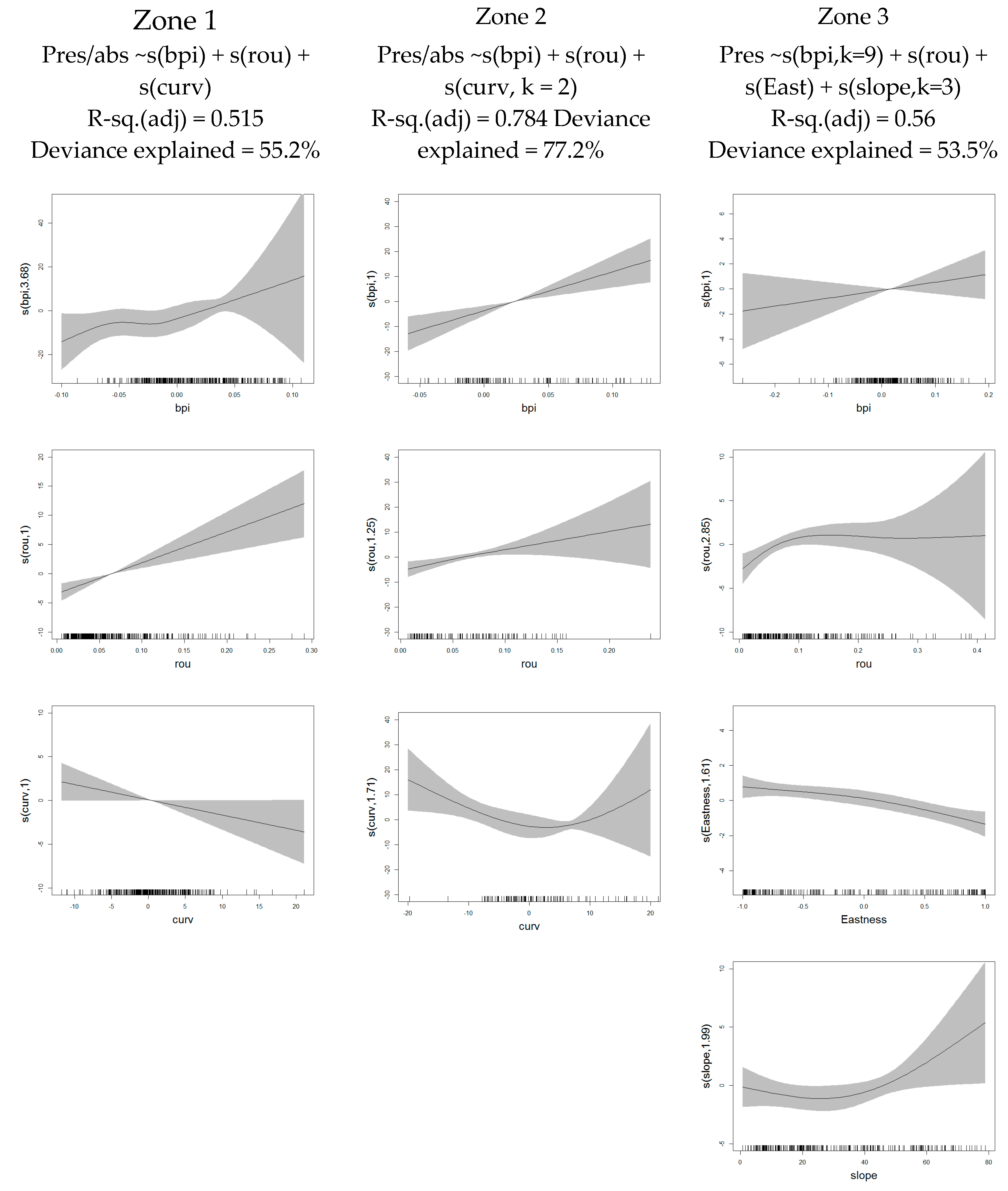
| R-sq.(adj)/Deviance Explained (%) | ||
|---|---|---|
| Terrain Variables | Zone 1 | Zone 2 |
| Aspect (North) | 0.014/2.54 | 0.01/0.22 |
| Aspect (East) | 0.015/2.8 | 0.02/4.36 |
| Bathymetric position index (BPI) | 0.320/38.7 | 0.45/43.7 |
| Curvature | 0.099/14.6 | 0.33/31.5 |
| Rugosity | 0.205/25.2 | 0.57/50.2 |
| Final model | 0.515/55.2 | 0.784/77.2 |
| AUC | 0.951 | 0.986 |
| R-sq.(adj)/Deviance Explained (%) | |||
|---|---|---|---|
| Terrain Variables | D. cornigera | A. transiens | P. ventilabrum |
| Northness | Not significant | 0.03/3.51 | 0.07/5.66 |
| Eastness | 0.1/8.14 | 0.03/2.6 | 0.28/22.8 |
| BPI | 0.11/11.1 | 0.2/16.4 | 0.26/22.6 |
| Curvature | 0.08/8.77 | 0.07/6.31 | 0.29/25.9 |
| Rugosity | 0.34/30.5 | 0.1/9.21 | 0.61/53.6 |
| Slope | 0.22/22.5 | 0.04/4.25 | 0.49/43.7 |
| Final model | 0.56/53.5 | 0.45/40.9 | 0.66/62.4 |
| AUC | 0.941 | 0.894 | 0.959 |
| Predicted | ||||||
|---|---|---|---|---|---|---|
| Truth | P. ventilabrum | D. cornigera | A. transiens | Background | Total | |
| P. ventilabrum | 54 | 0 | 0 | 8 | 62 | |
| D. cornigera | 0 | 145 | 0 | 68 | 213 | |
| A. transiens | 0 | 0 | 87 | 45 | 132 | |
| Background | 38 | 66 | 71 | – | 130 | |
| Total | 92 | 211 | 158 | 121 | – | |
| P. ventilabrum | D. cornigera | A. transiens | |
|---|---|---|---|
| True positives | 54 | 145 | 87 |
| False positives | 38 | 66 | 71 |
| False negatives | 8 | 68 | 45 |
| Precision | 0.59 | 0.69 | 0.55 |
| Recall | 0.87 | 0.68 | 0.66 |
| f1-score | 0.70 | 0.68 | 0.60 |
| Mean average precision | 0.61 | ||
| Mean recall | 0.74 | ||
| Mean f1-score | 0.66 | ||
© 2020 by the authors. Licensee MDPI, Basel, Switzerland. This article is an open access article distributed under the terms and conditions of the Creative Commons Attribution (CC BY) license (http://creativecommons.org/licenses/by/4.0/).
Share and Cite
Prado, E.; Rodríguez-Basalo, A.; Cobo, A.; Ríos, P.; Sánchez, F. 3D Fine-scale Terrain Variables from Underwater Photogrammetry: A New Approach to Benthic Microhabitat Modeling in a Circalittoral Rocky Shelf. Remote Sens. 2020, 12, 2466. https://doi.org/10.3390/rs12152466
Prado E, Rodríguez-Basalo A, Cobo A, Ríos P, Sánchez F. 3D Fine-scale Terrain Variables from Underwater Photogrammetry: A New Approach to Benthic Microhabitat Modeling in a Circalittoral Rocky Shelf. Remote Sensing. 2020; 12(15):2466. https://doi.org/10.3390/rs12152466
Chicago/Turabian StylePrado, Elena, Augusto Rodríguez-Basalo, Adolfo Cobo, Pilar Ríos, and Francisco Sánchez. 2020. "3D Fine-scale Terrain Variables from Underwater Photogrammetry: A New Approach to Benthic Microhabitat Modeling in a Circalittoral Rocky Shelf" Remote Sensing 12, no. 15: 2466. https://doi.org/10.3390/rs12152466
APA StylePrado, E., Rodríguez-Basalo, A., Cobo, A., Ríos, P., & Sánchez, F. (2020). 3D Fine-scale Terrain Variables from Underwater Photogrammetry: A New Approach to Benthic Microhabitat Modeling in a Circalittoral Rocky Shelf. Remote Sensing, 12(15), 2466. https://doi.org/10.3390/rs12152466