Identification of Urban Functional Areas by Coupling Satellite Images and Taxi GPS Trajectories

Abstract

Urban functional area (UFA) recognition is one of the most important strategies for achieving sustainable city development. As remote-sensing and social-sensing data sources have increasingly become available, UFA recognition has received a significant amount of attention. Research on UFA recognition that uses a single dataset suffers from a low update frequency or low spatial resolution, while data fusion-based methods are limited in efficiency and accuracy. This paper proposes an integrated model to identify UFA using satellite images and taxi global positioning system (GPS) trajectories in four steps. First, blocks were generated as spatial units in the study area, and the spatiotemporal information entropy of the taxi GPS trajectory (STET) for each block was calculated. Second, a 24-hour time-frequency series was formed based on the pick-up and drop-off points extracted from taxi trajectories and used as the interpretation indicator of the blocks. The K-Means++ and k-Nearest Neighbor (kNN) algorithm were used to identify their social functions. Third, a multilabel classification method based on the residual neural network (MLC-ResNets) and “You Only Look Once” (YOLO) target detection algorithms were used to identify the features of the typical and atypical spatial textures, respectively, of the satellite images in the blocks. The confidence scores of the features of the blocks were categorized by the decision tree algorithm. Fourth, to find the best way to integrate the two sub-models for UFA identification, the 10-fold cross-validation method based on stratified random sampling was applied to determine the most optimal STET thresholds. The results showed that the average accuracy reached 82.0%, with an average kappa of 73.5%—significant improvements over most existing studies. This paper provides new insights into how the advantages of satellite images and taxi trajectories in UFA identification can be fully exploited to support sustainable city management.

1. Introduction

Urban systems have natural and social characteristics. With rapid urbanization and the intensification of human activities, the structure and characteristics of the city have become more complex, and the types of urban functional areas (UFAs) more diverse [1]. Scientific planning of UFAs has become one of the important strategies for regional development and national construction [2], and the delineation of UFAs is essential for the optimization of urban planning [3]. In nature, each functional area is spatially aggregated by diverse geographic objects, which are semantically extracted from land uses [4,5]. Unlike the traditional investigation methods, the automatic and semiautomatic methods for mapping UFAs have been in high demand with the rapid development of geographical information and remote-sensing technologies. On the one hand, remote-sensing data have been widely used to detect Land Use and Land Cover (LULC) and built-up areas, with good effectiveness and efficiency. For instance, Landsat 8 is used to monitor land use changes [6,7], and the Luojia1-01 and Radiometer Suite (VIIRS) day-night band carried by the Suomi National Polar-orbiting Partnership (NPP) satellite have been used to extract urban built-up areas [8,9,10]. However, satellite images can only monitor the physical characteristics of a city’s land surface, and it is insufficient to recognize the social function and describe the spatiotemporal law of human mobility [11].

On the other hand, with the popularity of location-aware devices and related technologies, various types of social-sensing data have become available; these include vehicle trajectory data (e.g., those from taxis, bicycles and buses) [12,13,14]; social media sign-in data (e.g., Sina Weibo, Twitter and WeChat) [15,16,17]; points of interest and so on [18]. Based on these data, the laws of human mobility and the distribution pattern of the regional functions from the perspectives of time [19,20] and space [21,22] can be analyzed and established. However, due to the limitations of regional transportation, the economy and infrastructure construction, such sensing data, have not been fully available in all regions. The lack of social-sensing data makes it still difficult to accurately identify the type of UFAs [23].

In recent years, there has been a significant improvement in computer software and hardware [24]. Correspondingly, artificial intelligence (AI) algorithms have been implemented more easily, and a coupling analysis using multisource data has become a reality in the dynamic identification of UFAs [10,25]. AI enhances the methods of image recognition and contributes to the deeper mining of spatiotemporal laws. A multisource data coupling analysis can allow the advantages of the data themselves to be exploited and, furthermore, allow the data to complement each other. However, in the most recent research, multisource data have been directly input into an end-to-end artificial intelligence framework, which lacks the applicability of the evaluation and selection and may result in low accuracy and low efficiency.

A new integrated model for UFA identification is therefore proposed in this paper by coupling satellite images and taxi trajectory data and using AI algorithms. Firstly, an urban area was divided into blocks based on roads and rivers as the basic spatial units, and the spatiotemporal information entropy of the trajectory (STET) was calculated. A threshold was selected to divide the blocks into two groups based on STET. Then, two sub-models were developed to identify the functional types of the two groups of blocks using taxi GPS trajectories and satellite images. Based on the results of these two sub-models, a 10-fold cross-validation method based on stratified random sampling was used to adjust the threshold for determining the best way to integrate the two sub-models to obtain the best UFA identification strategy. The main innovations of this study include:

(1)

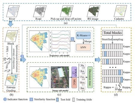
An integrated model of UFA identification was proposed. The functional type of some blocks was identified by the trajectory sub-model, while that of others was by the image sub-model. All these depend on the sufficiency of information of the trajectory data in the block. This new model can allow the advantages of social-sensing data and satellite images to be fully exploited and, thus, improves the identification accuracy.

(2)

A new index was designed and named STET, which was used as an index to measure the information of the trajectory data of blocks. A suitable sub-model was then selected to identify the UFA based on the STET index.

(3)

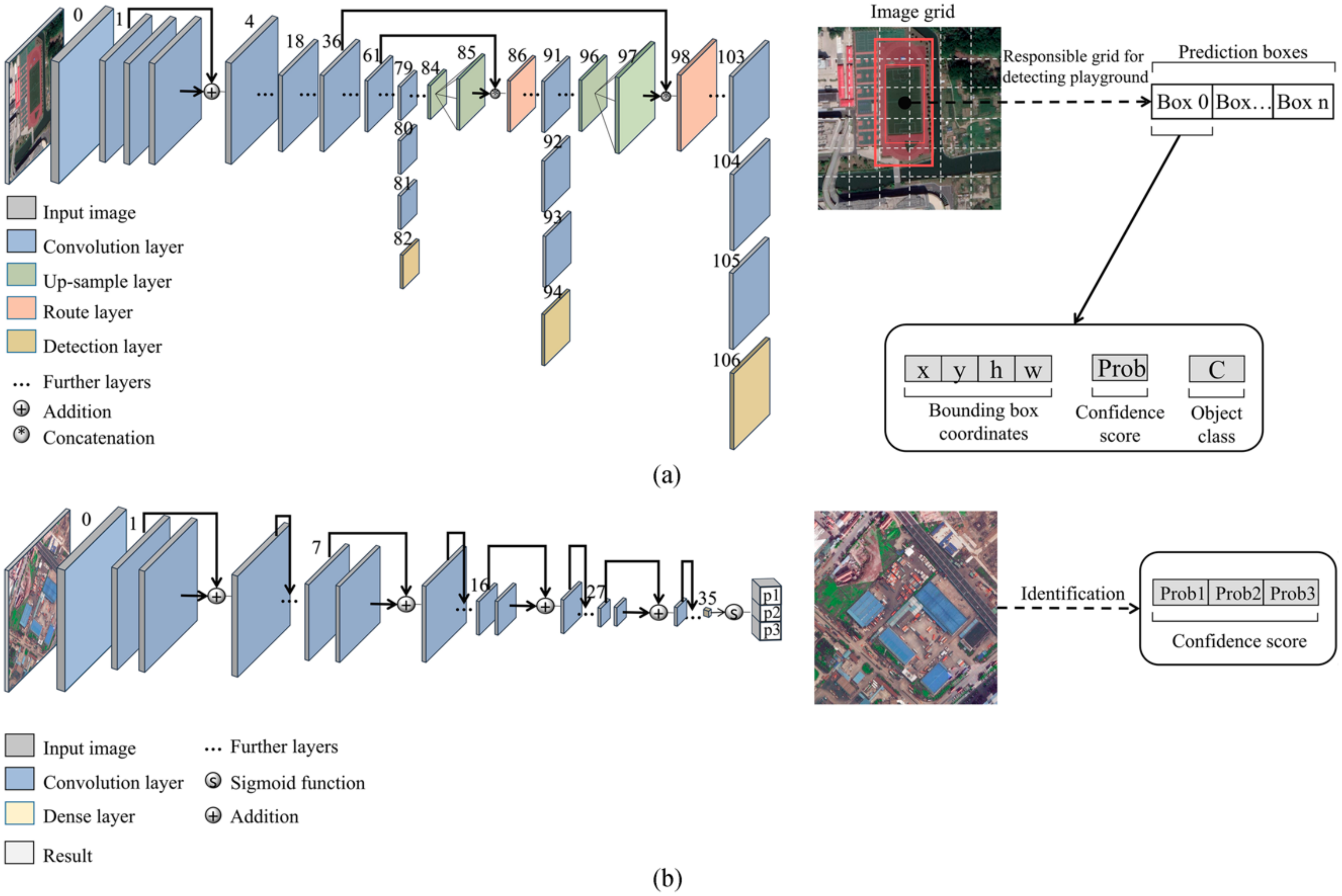
In the image sub-model, the multilabel classification method based on the residual neural network (MLC-ResNets) and You Only Look Once (YOLO) v3 algorithms were used to identify the land uses in the satellite image. Features with typical interpretation keys, such as schools, were identified using YOLO v3, while other features, such as residential areas, were identified using MLC-ResNets.

The rest of this paper is organized as follows. In Section 2, the study area and the dataset are briefly introduced. The methodology of the proposed model is illustrated in Section 3. The experimental results are presented and discussed in Section 4, and the conclusion is provided in Section 5.

2. Study Area and Datasets

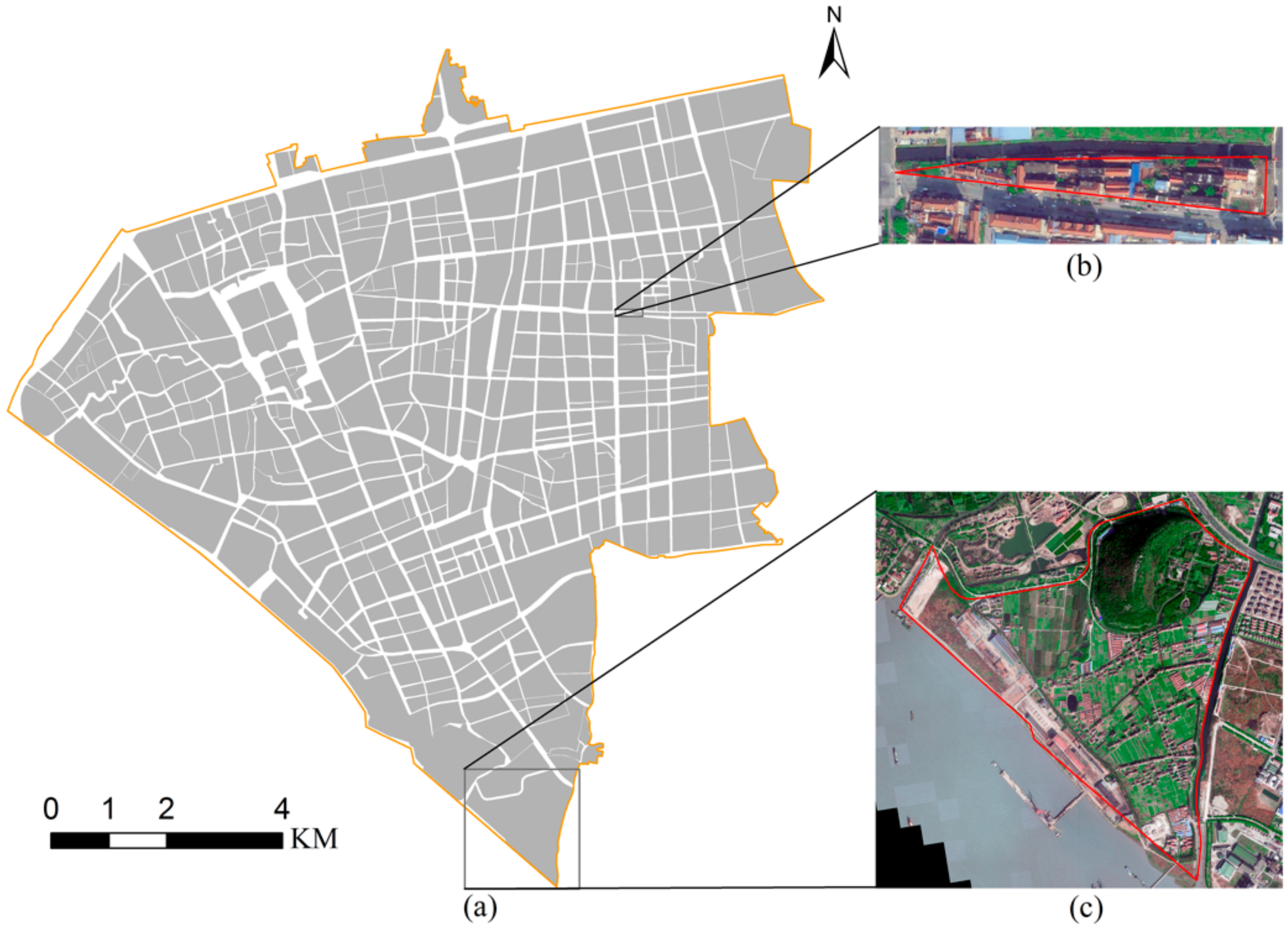
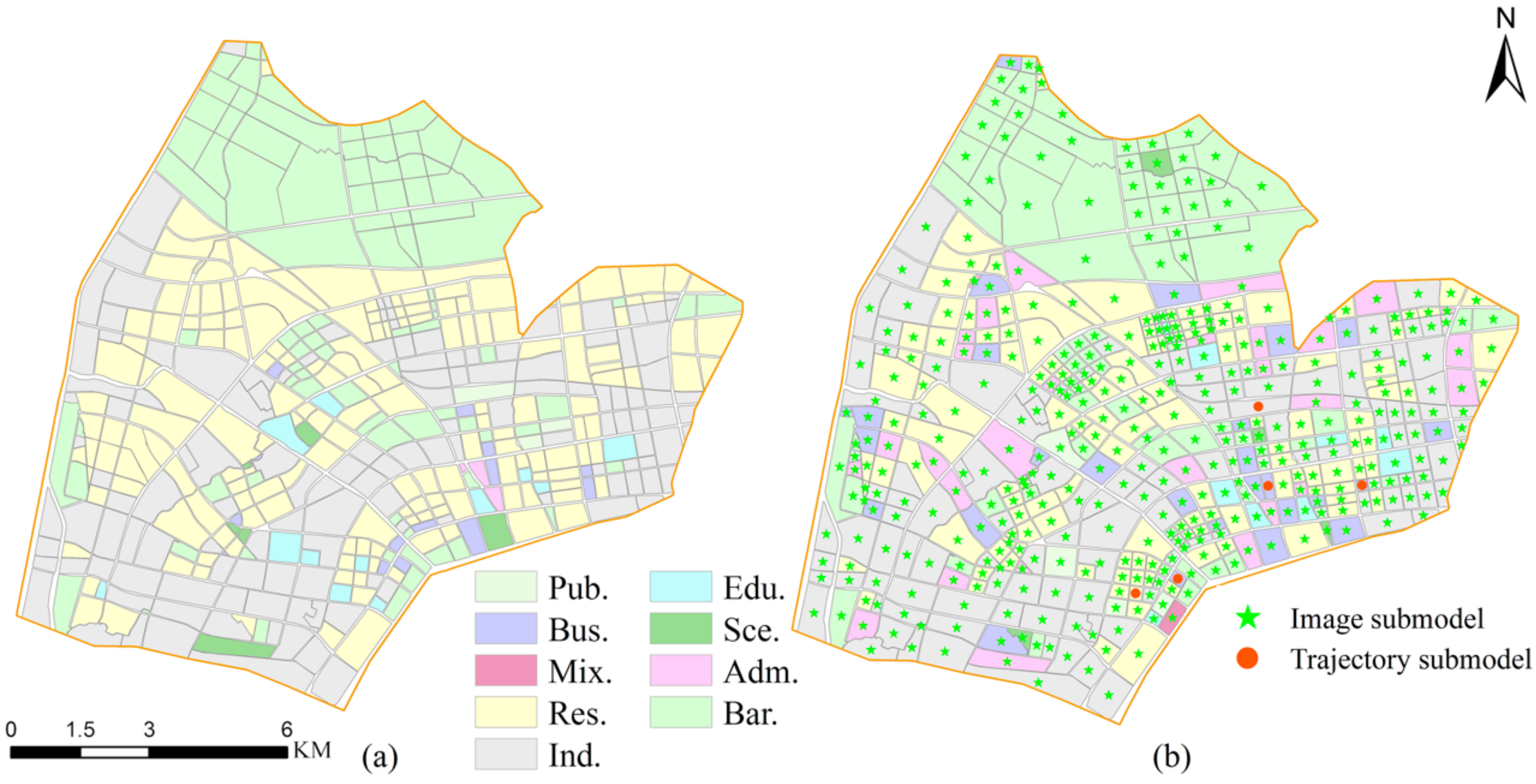
2.1. Study Area

The study area is Chongchuan District, located at 31°58’48”N, 120°53’42”E in Nantong on the Southeast coast of Jiangsu Province, China (Figure 1). This is where the Nantong Municipal Committee and Municipal Government are situated. The total area is around 215 square kilometers. In 2018, the resident population was 718,900, and the gross domestic product (GDP) was 81.951 billion Chinse Yuan. Since the subway in Nantong is yet to be constructed, taxis constitute one of the main travel modes for on-demand human mobility, with a total number of taxis of about 1200.

2.2. Datasets and Data Processing

Satellite images. This study uses satellite images from a Baidu map in 2018. The image has three RGB bands, with a resolution of 0.5 m/pixel. The preprocessing of the original image includes georeferencing and masking, as shown in Figure 2a. This image shows that the study area has a relatively higher proportion of construction land in the northwest and more green space in the east and south.

Taxi trajectory data. The GPS trajectory data, whose positioning mode is single-point positioning (SSP), are provided by the Nantong Taxi Management System from September, October and November 2018. The data are in a structured table file, which records the license plate number, phone number, time, longitude and latitude, speed, direction and passenger status. The sampling time interval is 30 s. The preprocessing includes the extraction of the pick-up and drop-off points, as shown in Figure 2b. The pick-up and drop-off points are determined by changes in the passenger status. When the status changes from empty to heavy, the point is the pick-up, while if it changes from heavy to empty, the point is the drop-off.

Road, rivers network and cadastral data. Other datasets include road, river and cadastral data. The road and river networks are obtained from a Baidu Map Application Programming Interface (API) using a web crawler, and the cadastral data are obtained from the Nantong City Planning Bureau (http://nantong.gov.cn/ntsghj/). Through data preprocessing, such as topology correction, georeferencing, line-to-polygon conversion, etc., other vector datasets are obtained, as shown in Figure 2c. To achieve greater geometric accuracy, the local coordinate projection system, GCS_China_Geodetic_Coordinate_System_2000, is used. The cadastral data (Figure 2d) include 9 functional types.

3. Methodology

This paper proposes an integrated model for UFA identification (Figure 3). In the first step, we combine the road and river networks to generate blocks as spatial units and calculate the spatiotemporal information entropy of trajectory (STET) for each block. Secondly, we use taxi trajectory data and satellite images to develop two sub-models to be optimized in the process of the UFA identification. If the STET is higher than or equal to the threshold $ϵ$, then the trajectory sub-model $\mathsf{\Psi }\left({\mathrm{T}}_{\mathrm{i}}\right)$ is used; otherwise, the image sub-model $\mathsf{\Phi }\left({\mathrm{I}}_{\mathrm{i}}\right)$ is used. Through the integrated model $\mathsf{\Gamma }\left({\mathrm{STET}}_{\mathrm{i}},{\mathrm{T}}_{\mathrm{i}},{\mathrm{I}}_{\mathrm{i}}\right)$, defined as Equation (1), the identification of the UFA of each block is implemented. Finally, due to the imbalance of the urban function types of the blocks, the 10-fold cross-validation based on stratified random sampling is used to adjust the threshold, and the accuracy and kappa coefficient are used to evaluate the effectiveness of the model. Figure 3 shows the research framework and related work.

$$\mathsf{\Gamma }\left({\mathrm{STET}}_{\mathrm{i}},{\mathrm{T}}_{\mathrm{i}},{\mathrm{I}}_{\mathrm{i}}\right)={\mathbb{I}}_{\left({\mathrm{STET}}_{\mathrm{i}}\ge ϵ\right)}\mathsf{\Psi }\left({\mathrm{T}}_{\mathrm{i}}\right)+{\mathbb{I}}_{({\mathrm{STET}}_{\mathrm{i}}<ϵ)}\mathsf{\Phi }\left({\mathrm{I}}_{\mathrm{i}}\right)\left(\mathrm{i}=1,2,\dots ,\mathrm{n}\right)$$

(1)

where n refers to the number of blocks, ${\mathrm{T}}_{\mathrm{i}}$ refers to the taxi trajectory data of block_i, ${\mathrm{I}}_{\mathrm{i}}$ refers to the satellite image of block_i and ${\mathbb{I}}_{\left(\mathrm{conditon}\right)}$ refers to the indicator function, whose value is 1 when the $\mathrm{condition}$ is true; otherwise, it is 0, and $ϵ$ refers to the decision threshold between using the trajectory sub-model or using the image sub-model.

3.1. Blocks and STET

3.1.1. Generation of Blocks

According to the United States (U.S.) Census Bureau’s definition of the block, a block is usually an area surrounded by humans and natural features, such as roads, rivers, lakes, mountains and cliffs [26]. It is the smallest granularity in urban planning and population statistics, so it is the smallest spatial unit in this study. Nantong is a city with developed traffic conditions along the river and sea. In this study, Nantong City is divided by a road network and river, generating several blocks. The road network and river have different levels. If the blocks are divided without distinguishing the levels, the block unit will be too small, which is inconsistent with the actual situation and will cause experimental difficulties. We recommend the roads and rivers of the third level for division, as shown in Figure 4, with a total of 482 blocks. The average area of the blocks is 17,3251${\mathrm{m}}^2$, ranging from the minimum area of 12,947${\mathrm{m}}^2$ to 1,730,130${\mathrm{m}}^2$. The urban function type of this block is mainly the residential area, which is composed of some rural houses, divided by the Tongjia River, Tongjia Road and Shengli Road, as shown in Figure 4b. The maximum area of the block is 1,730,130 ${\mathrm{m}}^2$. The urban function type of this block is mainly the industrial area, which is composed of Nantong Tongxin Village, Nantong COSCO Shipbuilding Steel Structure Co., Ltd., and many other factories, as shown in Figure 4c.

3.1.2. STET Computing

Information entropy reflects the capacity of information in the data. The larger the amount of information in the data, the greater the information entropy, and when $0<\mathrm{probability}\le \frac{1}{\mathrm{e}}$ (e refers to the basis of the natural logarithm and equals to 2.71), the entropy tends to increase [27]. When the social-sensing data in the study area are sufficient, the reliability of using the data to infer the functional type of the area is higher [28]. This paper proposes a measure of the trajectory information of the blocks—namely, the spatiotemporal information entropy of the trajectory (STET) of each block—defined as Equation (2). The STET is calculated from the density of the pick-up and drop-off points in the block at each period: $\mathrm{STET}\in \left(0,12.7\right]$. The higher the STET, the higher the traffic density of the block—that is, the block is a hotspot area.

$${\mathrm{STET}}_{\mathrm{i}}=-{\displaystyle \sum }_{\mathrm{j}=0}^{23}\frac{{\mathrm{N}}_{\mathrm{ij}}}{{\mathrm{S}}_{\mathrm{i}}}{\log }_2\frac{{\mathrm{N}}_{\mathrm{ij}}}{{\mathrm{S}}_{\mathrm{i}}}\left(\mathrm{i}=1,2,\dots ,\mathrm{n}\right)$$

(2)

where $\mathrm{n}$ refers to the number of blocks, ${\mathrm{N}}_{\mathrm{ij}}$ refers to the number of pick-up and drop-off points in block_i during the jth hour and ${\mathrm{S}}_{\mathrm{i}}$ refers to the area of block_i, which should be $\mathrm{e}$ times greater than ${\mathrm{N}}_{\mathrm{ij}}$ after standardization.

3.2. Trajectory-Based Sub-Model

Taxis constitute one of the main means by which residents travel in the study area on-demand, and its GPS trajectory data can thus perceive the spatiotemporal laws of residents’ travel behaviors. The spatiotemporal laws can effectively infer the distribution patterns of urban areas [19,20]. Therefore, when the trajectory data information is sufficient, no additional information needs to be added, and the trajectory sub-model $\mathsf{\Psi }\left({\mathrm{T}}_{\mathrm{i}}\right)$ can be used to mine the urban function type and spatial distribution pattern—that is, extract the time-frequency series of the pick-up and drop-off points of each block and use the K-Means++ and kNN algorithm to identify the social functions of the block.

3.2.1. Time Frequency Series and K-Means++

Time-frequency series. The time-frequency series of the pick-up and drop-off points extracted from the taxi trajectory can reflect the flow of information in different periods of the block. By mining the spatiotemporal laws of human activities, the urban functional attributes can be effectively inferred. In a recent study of the social functions of the area of interest (AOI), Zhou et al. (2019) proposed the concept of the hour-day spectrum (HDS) approach, which performed well in identifying the pattern of the social functions in Nantong [19]. The study proposed six kinds of spectrums, reflecting the regularity of the region’s changes over time. Since the taxi trajectories have a certain systematic error, in this paper, we generate block buffers according to the road widths [21] and generated the HDS for each block as a time-frequency sequence (Figure 5). The six spectrum types are: ${\mathrm{PP}}_{\mathrm{i}}=\left\{{\mathrm{pp}}_{\mathrm{i}0},\dots ,{\mathrm{pp}}_{\mathrm{ij}},\dots ,{\mathrm{pp}}_{\mathrm{i}23}\right\}$, which represents pick-up points; ${\mathrm{pp}}_{\mathrm{ij}}$, which represents the average number of pick-up points in the ith block during the jth hour; ${\mathrm{HPP}}_{\mathrm{i}}=\left\{{\mathrm{hpp}}_{\mathrm{i}0},\dots ,{\mathrm{hpp}}_{\mathrm{ij}},\dots ,{\mathrm{hpp}}_{\mathrm{i}23}\right\}$, which represents the pick-up points on holidays; ${\mathrm{WPP}}_{\mathrm{i}}=\left\{{\mathrm{wpp}}_{\mathrm{i}0},\dots ,{\mathrm{wpp}}_{\mathrm{ij}},\dots ,{\mathrm{wpp}}_{\mathrm{i}23}\right\}$, which represents the pick-up points on weekdays; ${\mathrm{DP}}_{\mathrm{i}}=\left\{{\mathrm{dp}}_{\mathrm{i}0},\dots ,{\mathrm{dp}}_{\mathrm{ij}},\dots ,{\mathrm{dp}}_{\mathrm{i}23}\right\}$, which represents the drop-off points; ${\mathrm{HDP}}_{\mathrm{i}}=\left\{{\mathrm{hdp}}_{\mathrm{i}0},\dots ,{\mathrm{hdp}}_{\mathrm{ij}},\dots ,{\mathrm{hdp}}_{\mathrm{i}23}\right\}$, which represents the drop-off points on holidays and ${\mathrm{WDP}}_{\mathrm{i}}=\left\{{\mathrm{wdp}}_{\mathrm{i}0},\dots ,{\mathrm{wdp}}_{\mathrm{ij}},\dots ,{\mathrm{wdp}}_{\mathrm{i}23}\right\}$, which represents the drop-off points on weekdays.

With the difference in the block popularity or grade [19], although the trend of the HDS in the same type of block is almost the same, the numerical magnitude of the sequence is different, so normalization is required. This article uses Equation (3) to normalize the 6 kinds of HDS in various blocks:

$${\mathrm{HDS}}_{\mathrm{iz}}^{\prime }=\frac{{\mathrm{HDS}}_{\mathrm{iz}}-\min \left({\mathrm{HDS}}_{\mathrm{iz}}\right)}{\max \left({\mathrm{HDS}}_{\mathrm{iz}}\right)-\min \left({\mathrm{HDS}}_{\mathrm{iz}}\right)}\left(\mathrm{i}=1,2,\dots ,\mathrm{n},\mathrm{z}=1,2,\dots ,6\right)$$

(3)

where $\mathrm{n}$ refers to the number of blocks; ${\mathrm{HDS}}_{\mathrm{iz}}$ refers to the zth HDS (PP, HPP, WPP, DP, HDP and WDP) of block_i; ${\mathrm{HDS}}_{\mathrm{iz}}^{\prime }$ refers to the normalized ${\mathrm{HDS}}_{\mathrm{iz}}$; $\max \left({\mathrm{HDS}}_{\mathrm{iz}}\right)$ refers to the maximum value in ${\mathrm{HDS}}_{\mathrm{iz}}$ and $\min \left({\mathrm{HDS}}_{\mathrm{iz}}\right)$ refers to the minimum value in ${\mathrm{HDS}}_{\mathrm{iz}}$.

K-Means++. Clustering algorithms are usually classified into partition-based, density-based and hierarchy-based types [29,30,31], among which the density-based clustering algorithm is often used to find data with density distribution features. It is not suitable for scattered data, and it has difficulty adjusting the parameters using prior knowledge from experiments [30]. The hierarchical clustering algorithm can partition data adaptively, but the model is inefficient and time-consuming [32]. The K-Means algorithm, as the representative of the partitioning data, has the advantages of effectively processing large data and high-dimensional data [33]. Compared with the K-Means algorithm, the K-Means++ algorithm optimizes the selection of clustering centers and reduces the impact of a poor selection of clustering centers [34]. The algorithm process is as follows: K samples are randomly selected as the clustering center,$\mathrm{CC}=\left\{{\mathrm{cc}}_1,{\mathrm{cc}}_2,\dots ,{\mathrm{cc}}_{\mathrm{k}}\right\}$, ensuring that the distance between each cluster center is relatively far. The distance (similarity) between each cluster center and each sample ${\mathrm{x}}_{\mathrm{i}}$ is calculated. Each sample is classified as the nearest (highest similarity) cluster center. The mean value among the cluster samples is calculated as the cluster center. Then, one cycles through the abovementioned operations until the cluster center does not change or the maximum number of iterations is reached. The K-Means++ algorithm has two most important factors—namely, the measure of similarity between data and the number of clusters.

3.2.2. Clustering Analysis

We use Euclidean distance as the K-Means++ similarity index ${\mathrm{S}}_{\mathrm{iz}}$, which is defined as Equation (4).

$${\mathrm{S}}_{\mathrm{iz}}={\displaystyle \sum }_{\mathrm{z}=1}^6\Vert {\mathrm{HDS}}_{\mathrm{iz}}^{\prime }-{\mathrm{cc}}_{\mathrm{kz}}\Vert {}_2\left(\mathrm{i}=1,2,\dots ,\mathrm{n},\mathrm{k}=1,2,\dots ,\mathrm{K}\right)$$

(4)

where $\mathrm{n}$ refers to the number of blocks; $\mathrm{K}$ refers to the number of clusters and ${\mathrm{cc}}_{\mathrm{kz}}$ refers to the zth HDS (PP, HPP, WPP, DP, HDP and WDP) of the kth cluster center.

The number of K-Means++ clusters often depends on the external prior experience or internal aggregation indicators in the data [35]. In remote-sensing fields, when unsupervised methods are used to classify land use, scholars often set the number of initial classifications to 2 to 3 times the final result [36]. In similar studies, the silhouette coefficient or elbow method is used to determine the number of classifications. While these methods can measure the aggregation between samples and give a reasonable number of classifications, in fact, the number is lower than the actual number of categories, so only coarser-grained classifications can be performed, which is not convenient for more detailed work [37]. Therefore, we will use external prior empirical methods to determine the number of classification categories.

After clustering is completed, each cluster may contain multiple functional types, so we need to identify the UFA type represented by each cluster—that is, the clusters of the same urban functional types are merged based on the maximum proportion principle, which is defined as Equation (5).

$${\mathrm{L}}_{{\mathrm{C}}_{\mathrm{k}}}^{\prime }=\underset{\mathrm{x}\in {\mathrm{L}}_{{\mathrm{c}}_{\mathrm{k}}}}{\mathrm{argmax}}\left(\frac{{\mathrm{n}}_{\mathrm{x}}}{{\mathrm{n}}_{{\mathrm{c}}_{\mathrm{k}}}}\right)\left(\mathrm{k}=1,2,\dots ,\mathrm{K}\right)$$

(5)

where ${\mathrm{c}}_{\mathrm{k}}$ refers to the k^th cluster, ${\mathrm{L}}_{{\mathrm{C}}_{\mathrm{k}}}^{\prime }$ refers to the original social functional attribute set of ${\mathrm{c}}_{\mathrm{k}}$, $\mathrm{K}$ refers to the number of clusters, ${\mathrm{L}}_{{\mathrm{c}}_{\mathrm{k}}}$ refers to the final social functional attributes of ${\mathrm{c}}_{\mathrm{k}}$, $\mathrm{x}$ refers to the social functional attribute element of ${\mathrm{c}}_{\mathrm{k}}$ and ${\mathrm{n}}_{\mathrm{x}}$ refers to the number of blocks with social functional attribute $\mathrm{x}$.

After the K-Means++ training is completed, the kNN algorithm is used to classify the unknown data in combination with the classified results. Specifically, the similarity between each test datum and each classified datum is calculated, and the similarity index is shown in Equation (4). Degrees are sorted in ascending order. The top k categories of data with the lowest similarity to the test data are used as their categories.

3.3. Image-Based Sub-Model

When the trajectory and other social-sensing data cannot provide effective decisions due to insufficient information, the satellite image is the most effective way to identify UFA types. We can mine UFA types and morphological patterns based on the image sub-model $\mathsf{\Phi }\left({\mathrm{I}}_{\mathrm{i}}\right)$, with the detection of the distribution patterns of some characteristic landmarks or buildings in the area. That is, MLC-ResNets and YOLO v3 are used to identify the block image, and the confidence score and other information are generated. Based on the identification results, the decision tree algorithm is used to classify the UFA types.

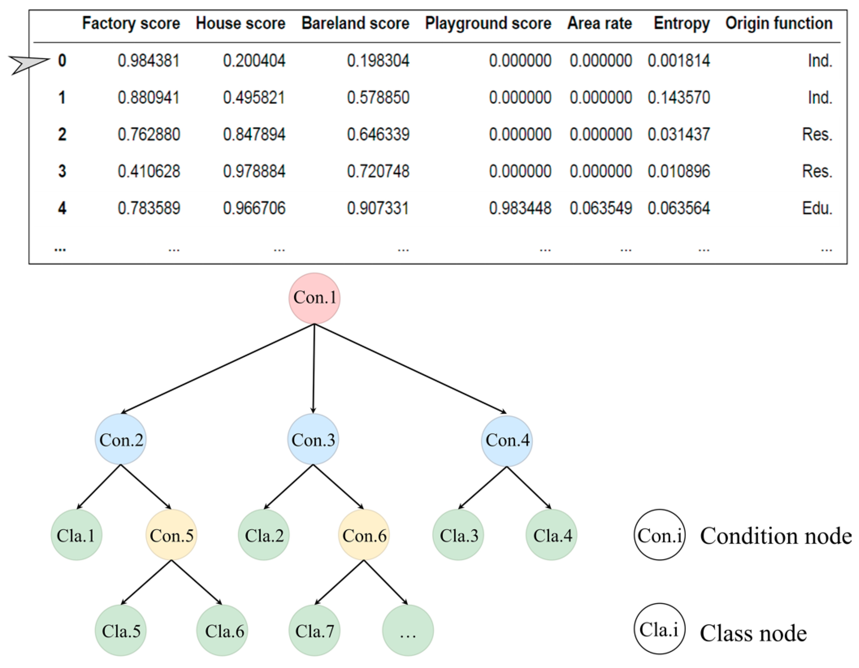
3.3.1. MLC-ResNets, YOLO v3 and Decision Tree

1. MLC-ResNets

Compared with the classification of satellite images based on spectral features, convolutional neural networks can simulate human vision and make classifications based on the physical shape and texture features of images, and this has played an important role in modern computer vision [38,39,40,41]. ResNets has proved to be an important breakthrough in the field of deep learning in recent years. It is characterized by the addition of internal residual blocks using jump connections, which are easy to optimize and whose accuracy can be increased by adding more layers [42]. In the blocks with multiple feature types, for example, a block may include residential areas, factories, schools, etc. The general classification task will consider the block as one of them, and the multilabel classification task refers to a series of nonexclusive labels on blocks according to the probability distribution of the features. The result of a probability distribution is ${\mathsf{\Phi }}_{\mathrm{m}}\left(\mathrm{I}\right)=\left\{{\mathrm{p}}_{\mathrm{m}}{}_1,\dots ,{\mathrm{p}}_{\mathrm{m}}{}_{\mathrm{l}},\dots ,{\mathrm{p}}_{\mathrm{m}}{}_{\mathrm{n}}\right\}$, where ${\mathrm{p}}_{\mathrm{m}}{}_{\mathrm{l}}$ is the confidence score of the feature in the image I.

In essence, the task of multilabel classification is to make a binary classification for each label. Therefore, when performing MLC-ResNets, the activation function at the end of the network needs to be set to the Sigmoid function, which has a value range of (0, 1) and is defined as Equation (6). The calculation result is often used to indicate the probability of things happening [43]. The loss function is set as the binary cross entropy, which is often used to measure the difference between two probability distributions and whether the model learning is sufficient. It is often combined with Sigmoid [44], and the combination is defined as Equation (7).

$$\mathsf{\sigma }\left(\mathrm{z}\right)=\frac{1}{1+{\mathrm{e}}^{-\mathrm{z}}}$$

(6)

where $\mathsf{\sigma }\left(\mathrm{z}\right)$ refers to Sigmoid function, $\mathrm{z}$ refers to the linear combination of the last layer input of the network and e refers to the basis of the natural logarithm (e = 2.71).

$$\mathrm{J}\left(\mathsf{\theta }\right)=-\left[{\displaystyle \sum }_{\mathrm{i}=1}^{\mathrm{N}}{\mathrm{y}}^{\left(\mathrm{i}\right)}{\mathrm{logh}}_{\mathsf{\theta }}\left({\mathrm{x}}^{\left(\mathrm{i}\right)}\right)+\left(1-{\mathrm{y}}^{\left(\mathrm{i}\right)}\right)\log (1-{\mathrm{h}}_{\mathsf{\theta }}\left({\mathrm{x}}^{\left(\mathrm{i}\right)}\right)\right]$$

(7)

where $\mathrm{J}\left(\mathsf{\theta }\right)$ refers to the loss function, $\mathrm{N}$ refers to the sample size, ${\mathrm{x}}^{\left(\mathrm{i}\right)}$ refers to the ith sample, ${\mathrm{h}}_{\mathsf{\theta }}\left({\mathrm{x}}^{\left(\mathrm{i}\right)}\right)$ refers to the activation function, which can be set to the Sigmoid function, and ${\mathrm{y}}^{\left(\mathrm{i}\right)}$ refers to the label of the ith sample.

2. YOLO v3

Some UFAs contain some typical geographic features, which can be used to infer the functional types of the areas, so these objects need to be detected based on satellite images. Recently, major breakthroughs have been made in object-detection algorithms in computer vision. The “You Only Look Once” (YOLO) algorithm is the representative one, which has a high performance and provides end-to-end prediction. YOLO v3, as the third generation of the YOLO algorithm, compared with the previous two generations, has a significantly improved classification accuracy and calculation speed and is suitable for detecting geographical entities that are not clustered [45,46,47,48]. The result is ${\mathsf{\Phi }}_{\mathrm{y}}\left(\mathrm{I}\right)$=$\left\{{\mathrm{p}}_{\mathrm{y}}{}_1,\dots ,{\mathrm{p}}_{\mathrm{y}}{}_{\mathrm{l}},\dots ,{\mathrm{p}}_{\mathrm{y}}{}_{\mathrm{n}}\right\}$, where ${\mathrm{p}}_{\mathrm{y}}{}_{\mathrm{l}}$ is the confidence score of target l in image I. The YOLO v3 algorithm uses a deep residual network to extract a series of multifeature layers of different sizes from the original picture and uses up-sampling to connect each feature layer. The network is trained by optimizing the comprehensive loss function, defined as Equations (8)–(13), to adjust the size, e.g., the width (w); height (h) and position, e.g., central coordinates (x, y) and category confidence (C) of the prior frame [47].

$$\mathrm{Loss}={\mathrm{Loss}}_1+{\mathrm{Loss}}_2+{\mathrm{Loss}}_3+{\mathrm{Loss}}_4+{\mathrm{Loss}}_5)$$

(8)

$${\mathrm{Loss}}_1={\displaystyle \sum }_{\mathrm{i}=0}^{{\mathrm{S}}^2}{\displaystyle \sum }_{\mathrm{j}=0}^{\mathrm{B}}{\mathrm{I}}_{\mathrm{ij}}^{\mathrm{obj}}\left[{\left({\mathrm{x}}_{\mathrm{i}}^{\mathrm{j}}-{\hat{\mathrm{x}}}_{\mathrm{i}}^{\mathrm{j}}\right)}^2+{\left({\mathrm{y}}_{\mathrm{i}}^{\mathrm{j}}-{\hat{\mathrm{y}}}_{\mathrm{i}}^{\mathrm{j}}\right)}^2\right]$$

(9)

$${\mathrm{Loss}}_2={\displaystyle \sum }_{\mathrm{i}=0}^{{\mathrm{S}}^2}{\displaystyle \sum }_{\mathrm{j}=0}^{\mathrm{B}}{\mathrm{I}}_{\mathrm{ij}}^{\mathrm{obj}}\left[{\left(\sqrt{{\mathrm{w}}_{\mathrm{i}}^{\mathrm{j}}}-\sqrt{{\hat{\mathrm{w}}}_{\mathrm{i}}^{\mathrm{j}}}\right)}^2+{\left(\sqrt{{\mathrm{h}}_{\mathrm{i}}^{\mathrm{j}}}-\sqrt{{\hat{\mathrm{h}}}_{\mathrm{i}}^{\mathrm{j}}}\right)}^2\right]$$

(10)

$${\mathrm{Loss}}_3=-{\displaystyle \sum }_{\mathrm{i}=0}^{{\mathrm{S}}^2}{\displaystyle \sum }_{\mathrm{j}=0}^{\mathrm{B}}{\mathrm{I}}_{\mathrm{ij}}^{\mathrm{obj}}\left[{\hat{\mathrm{C}}}_{\mathrm{i}}^{\mathrm{j}}\log \left({\mathrm{C}}_{\mathrm{i}}^{\mathrm{j}}\right)+(1-{\hat{\mathrm{C}}}_{\mathrm{i}}^{\mathrm{j}})\log \left(1-{\mathrm{C}}_{\mathrm{i}}^{\mathrm{j}}\right)\right]$$

(11)

$${\mathrm{Loss}}_4=-{\mathsf{\lambda }}_{\mathrm{noobj}}{\displaystyle \sum }_{\mathrm{i}=0}^{{\mathrm{S}}^2}{\displaystyle \sum }_{\mathrm{j}=0}^{\mathrm{B}}{\mathrm{I}}_{\mathrm{ij}}^{\mathrm{noobj}}\left[{\hat{\mathrm{C}}}_{\mathrm{i}}^{\mathrm{j}}\log \left({\mathrm{C}}_{\mathrm{i}}^{\mathrm{j}}\right)+(1-{\hat{\mathrm{C}}}_{\mathrm{i}}^{\mathrm{j}})\log \left(1-{\mathrm{C}}_{\mathrm{i}}^{\mathrm{j}}\right)\right]$$

(12)

$${\mathrm{Loss}}_5=-{\displaystyle \sum }_{\mathrm{i}=0}^{{\mathrm{S}}^2}{\mathrm{I}}_{\mathrm{ij}}^{\mathrm{obj}}{\displaystyle \sum }_{\mathrm{c}\in \mathrm{classes}}\left[{\hat{\mathrm{P}}}_{\mathrm{i}}^{\mathrm{j}}\log \left({\mathrm{P}}_{\mathrm{i}}^{\mathrm{j}}\right)+\left(1-{\hat{\mathrm{P}}}_{\mathrm{i}}^{\mathrm{j}}\right)\log \left(1-{\mathrm{P}}_{\mathrm{i}}^{\mathrm{j}}\right)\right]$$

(13)

where ${\mathrm{Loss}}_1,{\mathrm{Loss}}_2,{\mathrm{Loss}}_3,{\mathrm{Loss}}_4\mathrm{and} {\mathrm{Loss}}_5$ refer to the central coordinate error, width height coordinate error, object confidence error, no object confidence error and classification error, respectively. ${\mathrm{I}}_{\mathrm{ij}}^{\mathrm{obj}}$ refers to whether the jth anchor box of the ith grid is responsible for this object. If it is, ${\mathrm{I}}_{\mathrm{ij}}^{\mathrm{obj}}=1$; otherwise, it is 0. $\mathrm{S}$ refers to the number of grids. $\mathrm{B}$ refers to the number of anchor boxes. ${\mathrm{x}}_{\mathrm{i}}^{\mathrm{j}}$ and ${\mathrm{y}}_{\mathrm{i}}^{\mathrm{j}}$ refer to the central coordinate of the jth anchor box of the ith grid. ${\hat{\mathrm{x}}}_{\mathrm{i}}^{\mathrm{j}}$ and ${\hat{\mathrm{y}}}_{\mathrm{i}}^{\mathrm{j}}$ refer to the predicted central coordinate of the jth anchor box of the ith grid. ${\mathrm{w}}_{\mathrm{i}}^{\mathrm{j}}$ and ${\mathrm{h}}_{\mathrm{i}}^{\mathrm{j}}$ refer to the width and height of the jth anchor box of the ith grid. ${\hat{\mathrm{w}}}_{\mathrm{i}}^{\mathrm{j}}$ and ${\hat{\mathrm{h}}}_{\mathrm{i}}^{\mathrm{j}}$ refer to the predicted width and height of the jth anchor box of the ith grid. ${\mathrm{C}}_{\mathrm{i}}^{\mathrm{j}}$ refers to the category confidence of the jth anchor box of the ith grid. ${\hat{\mathrm{C}}}_{\mathrm{i}}^{\mathrm{j}}$ refers to the predicted category confidence of the jth anchor box of the ith grid. ${\mathrm{P}}_{\mathrm{i}}^{\mathrm{j}}$ refers to the classification accuracy of the object of the jth anchor box of the ith grid. ${\hat{\mathrm{P}}}_{\mathrm{i}}^{\mathrm{j}}$ refers to the predicted classification accuracy of the object of the jth anchor box of the ith grid. ${\mathsf{\lambda }}_{\mathrm{noobj}}$ refers to penalty coefficient of ${\mathrm{Loss}}_4$.

3. Decision Tree

In the case of insufficient trajectory information, ${\mathsf{\Phi }}_{\mathrm{m}},{\mathsf{\Phi }}_{\mathrm{y}}$ is used to mine useful information from the satellite image and calculate the confidence score of each type of object: ${\mathrm{P}}_{\mathrm{i}}=\left\{{\mathsf{\Phi }}_{\mathrm{m}}\left({\mathrm{I}}_{\mathrm{i}}\right),{\mathsf{\Phi }}_{\mathrm{y}}\left({\mathrm{I}}_{\mathrm{i}}\right)\right\}$. Then, we combine with the traditional machine-learning algorithms ${\mathsf{\Phi }}_{\mathrm{t}}$ to learn the classification of the hidden mode—namely, $\mathsf{\Phi }\left({\mathrm{I}}_{\mathrm{i}}\right)={\mathsf{\Phi }}_{\mathrm{t}}\left({\mathrm{P}}_{\mathrm{i}}\right)$.

Decision tree is a supervised classification method, which is based on a tree structure and has the advantages of high readability and speed. Decision tree usually consists of three steps: feature selection, tree generation and overfitting processing [49]. Feature selection belongs to feature engineering—namely, selecting reasonable and classifiable features for learning. The ID3 algorithm is often employed in the generation of a decision tree in the following way: starting from the root node, all possible information divergence is calculated, as defined in Equation (14). The greatest feature of the information divergence, its node characteristics, is set up by the characteristics of the node child nodes. These steps are repeated until the information divergence is small, or there are no features to choose from.

$$\mathrm{g}\left(\mathrm{D},\mathrm{A}\right)=-{\displaystyle \sum }_{\mathrm{j}=1}^{\mathrm{m}}\frac{\left|{\mathrm{C}}_{\mathrm{j}}\right|}{\left|\mathrm{D}\right|}{\log }_2\frac{\left|{\mathrm{C}}_{\mathrm{j}}\right|}{\left|\mathrm{D}\right|}+{\displaystyle \sum }_{\mathrm{i}=1}^{\mathrm{n}}\frac{\left|{\mathrm{D}}_{\mathrm{i}}\right|}{\left|\mathrm{D}\right|}{\displaystyle \sum }_{\mathrm{j}=1}^{\mathrm{m}}\frac{\left|{\mathrm{C}}_{\mathrm{ij}}\right|}{\left|{\mathrm{D}}_{\mathrm{i}}\right|}{\log }_2\frac{\left|{\mathrm{C}}_{\mathrm{ij}}\right|}{\left|{\mathrm{D}}_{\mathrm{i}}\right|}$$

(14)

where $\mathrm{D}$ refers to the dataset, A refers to the feature, m refers to the number of labels, $\left|C_j\right|$ refers to the number of samples belonging to the jth label, $\left|\mathrm{D}\right|$ refers to the number of samples, n refers to the number of features, $\left|{\mathrm{D}}_{\mathrm{i}}\right|$ refers to the number of samples of the ith feature and $\left|{\mathrm{C}}_{\mathrm{ij}}\right|$ refers to the number of samples of the ith feature belonging to the jth label.

The decision tree generation algorithm will generate the decision tree recursively, which leads to a high accuracy of the training set but a weak generalization ability. In other words, overfitting easily occurs, and it can be prevented by pruning or limiting the depth of the tree.

3.3.2. Image Analysis

Based on the field investigation and the prior background knowledge of Nantong, we found that most of the blocks that meet the requirements of the image sub-model are almost all factories, bare/farmland, rural land, nonopen schools and residential areas under construction. Based on this background, we performed an image classification for these features, which can greatly simplify the workload and allow for a quick prediction of the urban functional categories of the blocks.

Before the classification task, we analyzed all kinds of other areas and selected the appropriate method of image classification: (1) The spatial distribution of the school does not have aggregation and contains representative ground features, such as a playground. By identifying the playground and calculating the area proportion of the playground, the school type can be inferred. YOLO v3 has a better recognition effect on such objects, so it is suitable to use as the target detection algorithm. (2) Since the physical characteristic of the factory and residential area are different and have spatial aggregation, it is difficult to use target detection, which is suitable for multitarget classification. (3) The spatial extent of bare/farmland, which is often used as a background area, is large, and the probability of residential factories can be compared to determine whether it belongs to this type. It is suitable for multi-objective classification tasks. Therefore, we identified playgrounds, factories, residential areas and bare/farmland as targets. Figure 6 shows the structure of YOLO v3 and MLC-ResNets.

After the classification based on the deep-learning algorithm, the confidence result of the target feature and the area proportion of the playground are obtained. Combined with the STET and the actual UFA type, the structured dataset is constructed, and classification learning experiments are conducted using the decision tree algorithm, as shown in Figure 7.

3.4. Model Verification Method

3.4.1. Stratified Random Sampling

Stratified random sampling first divides the overall samples into various types. Then, according to the ratio of the sample number of each type to the total number, the number of each type is determined. Finally, samples are drawn from each type according to the random principle. This method can ensure that, after data division, the proportion of categories in each dataset is consistent, and it is suitable for data with uneven sampling categories [50,51].

3.4.2. K-fold Cross-Validation

Cross-validation is often used to check the accuracy of the model. As the number of blocks is only a few, and the function type is unbalanced, it is easy to cause the verification results to be unrepresentative using simple cross-validation. Therefore, the applicable k-fold cross-validation divides the training set into k sub-samples, which means that a single sub-sample is reserved as the data of the validation model, and the other k-1 samples are used for training and are repeated k times. The average k-times result is used as the final estimation—among which, that of the 10-fold cross-validation is the most popular [52].

3.4.3. Kappa Coefficient

Kappa coefficient, defined as Equations (15–17), is used for consistency test the evaluation of the classification tasks of unbalanced data. Its value ranges from 0 to 1, of which 0.0 ~ 0.20 represents extremely low consistency, 0.21 ~ 0.40 represents general consistency, 0.41 ~ 0.60 represents moderate consistency, 0.61 ~ 0.80 represents high consistency and 0.81 ~ 1 represents almost complete consistency [53]. This index is often used in the study of land use classification in remote-sensing geoscience analyses.

$$\mathrm{k}=\frac{{\mathrm{p}}_{\mathrm{o}}-{\mathrm{p}}_{\mathrm{e}}}{1-{\mathrm{p}}_{\mathrm{e}}}$$

(15)

$${\mathrm{p}}_{\mathrm{o}}=\frac{{{\displaystyle \sum }}_{\mathrm{m}\in \mathrm{diag}\left(\mathrm{M}\right)}^{\mathrm{N}}\mathrm{m}}{{{\displaystyle \sum }}_{\mathrm{i}=1}^{\mathrm{N}}{{\displaystyle \sum }}_{\mathrm{j}=1}^{\mathrm{N}}{\mathrm{M}}_{\mathrm{ij}}}$$

(16)

$${\mathrm{p}}_{\mathrm{e}}=\frac{{{\displaystyle \sum }}_{\mathrm{i}=1}^{\mathrm{N}}{\mathrm{M}}_{\mathrm{i}·}·{\mathrm{M}}_{·\mathrm{i}}}{{\left({{\displaystyle \sum }}_{\mathrm{i}=1}^{\mathrm{N}}{{\displaystyle \sum }}_{\mathrm{j}=1}^{\mathrm{N}}{\mathrm{M}}_{\mathrm{ij}}\right)}^2}$$

(17)

where $\mathrm{N}$ refers to the number of samples, M refers to the confusion matrix, ${\mathrm{M}}_{\mathrm{i}·}$ refers to the ith row of M, ${\mathrm{M}}_{·\mathrm{i}}$ refers to the ith column of M, ${\mathrm{M}}_{\mathrm{ij}}$ refers to the value in the ith row and jth column of M and ${\mathrm{p}}_{\mathrm{o}}$ and ${\mathrm{p}}_{\mathrm{e}}$ refer to intermediate variables.

4. Results and Discussion

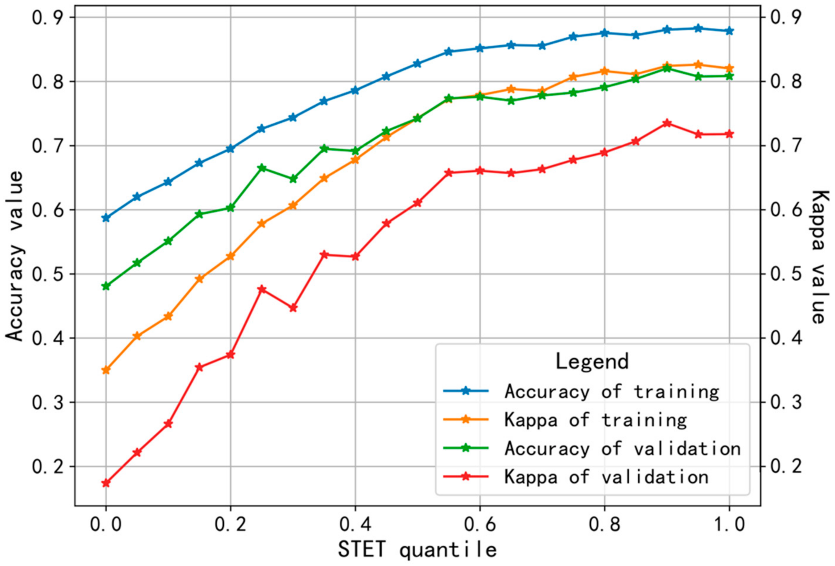
All experiments in this part are conducted on the Jupyter Notebook, ArcGIS software platform, GeForce RTX 2080ti GPU, and other hardware platforms and Python libraries, such as Numpy, Pandas, Keras and Matplotlib, are used. Basic information on all blocks is shown in

Table 1. Basic block information.

Block Function Type	Amount	Maximum Area (m2)	Minimum Area (m2)
Residential area	232	1,129,280	16,049
Business area	30	395,814	12,947
Education area	18	929,251	36,745
Industrial area	109	1,730,130	21,572
Administrative area	14	285,251	16,990
Public service area	6	359,814	32,541
Mixed area	5	320,808	180,431
Scenic spot	7	1,088,470	47,223
Bare/farmland	61	544,611	17,984

.

4.1. STET Analysis

Figure 8 shows the STET value of each block. For example, the STET of South Street (a), Central South Century City (b) and Nantong East Passenger Station (c) are higher, indicating that there are more residential activities in this block, and the trajectory information is sufficient. The marginal region of the study area is mainly industrial or rural, and the STET is lower, indicating that there are fewer residential activities in this area, and there is little trajectory information. The STET results present a right-skewed distribution, so it is difficult to directly select $ϵ$. Therefore, based on the quantile of STET as the value of $ϵ$, in the following experiments (4.2 and 4.3), we will take the 50% quantile of STET (i.e., the median, ϵ = 0.0983) as the default threshold and adjust $ϵ$ in Section 4.4 to select the optimal parameters of the model.

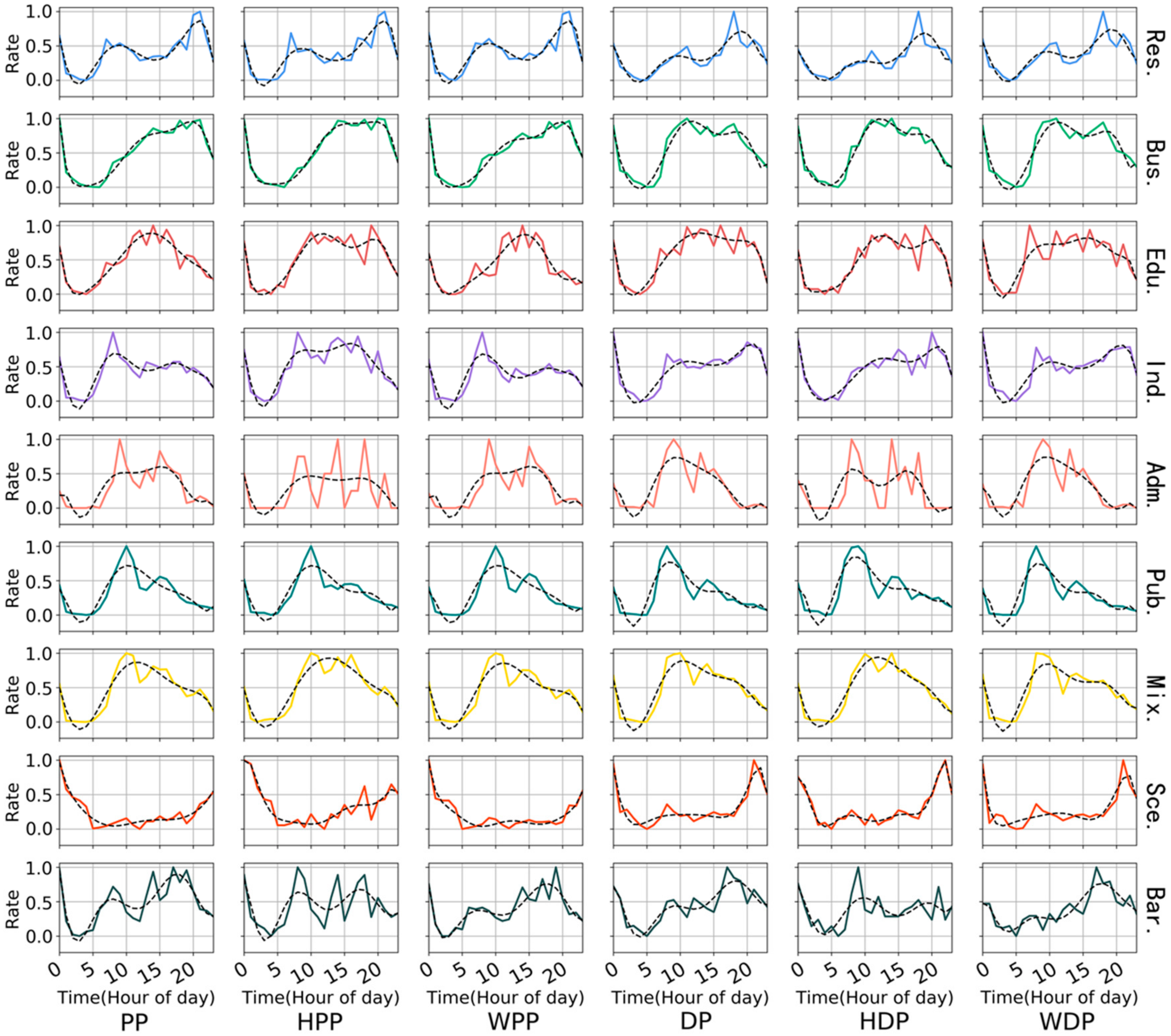
4.2. Results of the Trajectory Sub-Model

4.2.1. HDS Result

Figure 9 shows the HDS curves of different types of blocks, for which the $\mathrm{STET}$ values are greater than $ϵ$. It can be seen that different types of blocks have their unique spatiotemporal patterns, and there are some differences between the different types of HDS. Taking the business area as an example, the curves of the pick-up points show an upward trend from 6 a.m. to 10 p.m. and reach a peak at 10 p.m. This indicates that, with the time delay, residents leave the business area after shopping. On holidays, the curves are stable from 3 p.m. to 10 p.m. and are in a peak state, and on weekdays, the peak of the curve is often at 10 p.m., indicating that, during the holidays, residents have more free time to shop, while, on the weekdays, most of the residents shop after work. The curve of the drop-off points peaked at 10 a.m., indicating that most residents like shopping during this period. From 3 p.m. to 8 p.m., the curve of holidays is slightly higher than that of weekdays, which also confirms the difference between the above-mentioned residents’ work and rest on holidays and weekdays.

Figure 10 shows that there are differences between the HDS of different types of blocks, and the similarity confusion matrix is calculated by Equation (4) based on these HDS. The lower the value, the higher the similarity. Among them, the similarity between the administrative area and the public service area is high, which indicates that the spatiotemporal characteristics of the two functional districts are similar, and they can provide some services for residents. Secondly, the similarity between the mixed area and the business area, the education area and the public service area is high, which indicates that there may be business land or schools in the mixed area.

However, due to the difference in the UFA level and property of the blocks, taking the public service area as an example, hospitals, stations and gymnasiums all belong to this function type, while these three types have their spatiotemporal laws, which leads to a large difference in the HDS trend, as shown in Figure 11. In order to distinguish their differences in the trajectory sub-model, we again divide education areas, residential areas and public service areas in a fine-grained way, as shown in

Table 2. Different levels of the urban functional area (UFA).

Rude Grained Division	Fine Grained Division
Public service area	Hospital
	Station
	Gymnasium
Residential area	Residential quarters
	Countryside
Education area	Primary school
	Middle school
	College
	University

.

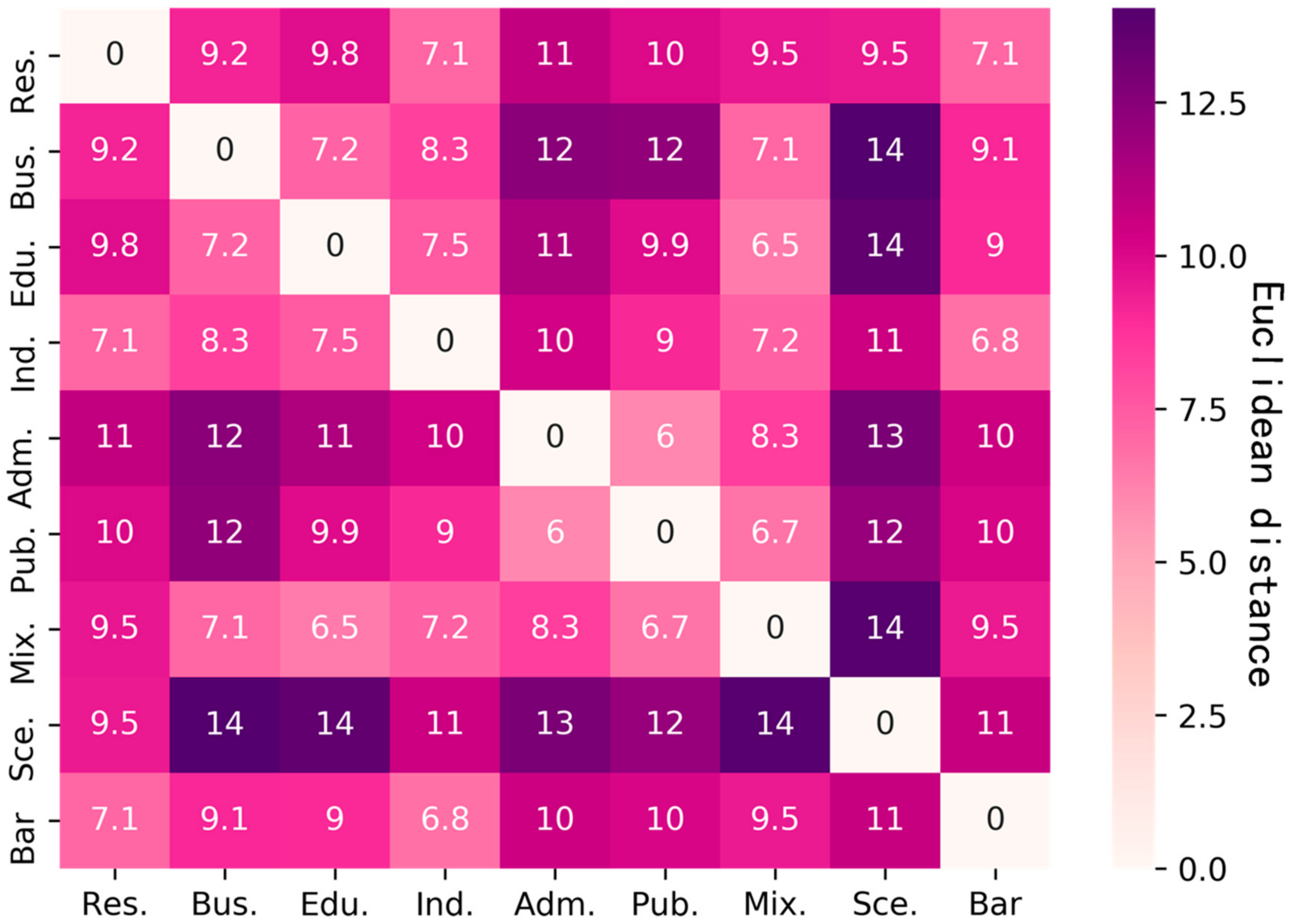
4.2.2. Cluster Result

Taking Equation (4) as the similarity index and three times the fine-grained UFA number as the initial classification number to train the trajectory sub-model, we use a stratified random sampling method to select 80% of the data for training and 20% of the data for validation. Combined with the real cadastral data, we count the proportion of the original types in each cluster and merge the clusters by the principle of the maximum proportion. The results are shown in

Table 3. Merging process of the clustering results.

Label	Res. Rate	Bus. Rate	Edu. Rate	Ind. Rate	Adm. Rate	Pub. Rate	Mix. Rate	Sce. Rate	Bar. Rate	Merge
1	75%	25%	0%	0%	0%	0%	0%	0%	0%	Res.
2	33%	11%	0%	11%	22%	22%	0%	0%	0%	Res.
3	80%	0%	0%	20%	0%	0%	0%	0%	0%	Res.
4	100%	0%	0%	0%	0%	0%	0%	0%	0%	Res.
5	69%	15%	0%	8%	8%	0%	0%	0%	0%	Res.
6	25%	0%	50%	25%	0%	0%	0%	0%	0%	Edu.
7	67%	0%	0%	11%	11%	0%	0%	0%	11%	Res.
…	…	…	…	…	…	…	…	…	…	…
39	17%	17%	50%	17%	0%	0%	0%	0%	0%	Edu.
40	50%	0%	0%	50%	0%	0%	0%	0%	0%	Res.
41	0%	0%	0%	0%	0%	100%	0%	0%	0%	Pub.
42	60%	0%	20%	20%	0%	0%	0%	0%	0%	Res.
43	75%	25%	0%	0%	0%	0%	0%	0%	0%	Res.
44	100%	0%	0%	0%	0%	0%	0%	0%	0%	Res.
45	75%	0%	0%	0%	0%	0%	0%	25%	0%	Res.

. Based on the results of the K-Means++ merging, the result is tested using the kNN algorithm. In this case, the accuracy and Kappa coefficient of the trajectory sub-model are 71% and 46%, respectively. Due to the low ϵ, the trajectory data information is insufficient, and the accuracy and kappa coefficient need to be improved. A comprehensive parameter adjustment is carried out in Section 4.4 in combination with the image model.

4.3. Results of the Image Sub-Model

The image recognition of UFA is a one-to-one process, which needs to be processed in blocks. Therefore, the satellite image of the block range that meets the conditions of the image model is used as the test sample, and part of the data is shown in Figure 12a. In this model, the education area, industrial area, residential area and bare/farmland are identified.

4.3.1. Image Classification Result

Nantong is located in the Middle-east of Jiangsu Province. Considering the differences in the natural and human landscapes between the different regions, we selected a large number of images from Jiangsu, Zhejiang and Shanghai as training samples downloaded from the Baidu Map, including 200 industrial area images, 200 residential area images, 200 bare/farmland images and 400 mixed-type images. Part of the training images are shown in Figure 12b. The training and test images, which have been resized into 300*300 pixels, are labeled and trained with the network architecture shown in Figure 6b. Figure 13a shows the learning status of the network. While the curve of the verification set fluctuates greatly, the overall trend is downward. After the 50th epoch, the model tends to overfitting—that is, the loss of validation decreases and then rises, so the model of 50 epochs training is more suitable.

Based on the same conditions, 400 pictures of the schools with playgrounds are selected as the training set. As shown in Figure 12c, the training samples are labeled and trained using the YOLO v3 network architecture of Figure 6a. Figure 13b shows the learning status of the network. The learning effect is good before the 90th epoch, and after that, the loss curve rises sharply, indicating that there is an exploding gradient problem. This is due to the large and complex structure of YOLO v3, which leads to the instability of the network weight update. Therefore, the model of 90 epochs training is adopted.

4.3.2. Decision Tree Result

After the recognition of the images, the confidence results of each image, the area rate of the playground and the STET value of the block are combined into a real category to establish a structured table. Taking part of the data shown in Figure 12a as an example, with its structured table shown in

Table 4. Structured table for the Decision Tree.

Image ID	True Category	STET	Confidence Score				Playground Area Rate
			Playground	Factory	House	Bare/farmland
1	Sce.	0.010	0.000	0.870	0.814	0.897	0.000
2	Res.	0.013	0.000	0.800	0.153	0.055	0.000
3	Ind.	0.014	0.000	0.963	0.632	0.587	0.000
4	Bar.	0.003	0.000	0.359	0.379	0.823	0.000
5	Ind.	0.001	0.000	0.915	0.521	0.646	0.000
6	Edu.	0.009	0.981	0.261	0.977	0.316	0.172
7	Ind.	0.002	0.000	0.969	0.194	0.264	0.000
8	Edu.	0.105	0.991	0.800	0.828	0.697	0.040
9	Res.	0.003	0.000	0.158	0.927	0.141	0.000
10	Res.	0.039	0.000	0.541	0.811	0.589	0.000
11	Ind.	0.027	0.000	0.998	0.126	0.185	0.000
12	Ind.	0.002	0.000	0.810	0.535	0.509	0.000
13	Res.	0.009	0.000	0.412	0.845	0.244	0.000
14	Ind.	0.008	0.000	0.997	0.053	0.058	0.000
15	Edu.	0.012	0.926	0.584	0.847	0.872	0.020
16	Edu.	0.039	0.987	0.180	0.972	0.050	0.045
17	Bar.	0.007	0.000	0.396	0.649	0.876	0.000
18	Res.	0.004	0.000	0.522	0.827	0.590	0.000
19	Bar.	0.004	0.319	0.590	0.644	0.973	0.107
20	Bar.	0.007	0.000	0.397	0.696	0.872	0.000
21	Res.	0.003	0.000	0.460	0.835	0.723	0.000
22	Res.	0.001	0.000	0.571	0.890	0.687	0.000
23	Res.	0.003	0.000	0.266	0.958	0.517	0.000
24	Ind.	0.048	0.000	0.935	0.466	0.578	0.000
25	Res.	0.003	0.000	0.491	0.908	0.536	0.000

, through the probability of geographic features and other information, the urban functional area of the corresponding block can be inferred. For example, when the confidence result of the playground and the area rate is large, the real type is mostly like the education area. The stratified random sampling method is used to select 80% of the blocks that meet the conditions of the image sub-model as the training set and 20% as the test set. The decision tree algorithm is used to learn based on the structured table. The decision tree algorithm easily encounters an overfitting problem, which can be prevented by adjusting the tree height parameters. As shown in Figure 14, the model works best when the tree height is 5, with a test accuracy of 85% and a Kappa coefficient of 79%.

4.4. Model Parameter Adjustment

In this section, we use the 10-fold cross-validation method based on stratified random sampling to integrate the trajectory sub-model and the image sub-model by adjusting the parameter to achieve the optimal effect of the recognition model. Figure 15 shows the identification results of the integrated model based on different STET quantiles. The learning curve of the model rises with the increase of $ϵ$. When the quantile reaches 90% (ϵ = 0.491), the identification effect of the model is the best, with an average test accuracy of 82.0% and kappa coefficient of 73.5%, which shows that the identification results are highly consistent, and the recognition effect of the model is poor under the condition of low data information. It is worth noting that, when the STET quantity = 0 or 1, this means that only the trajectory sub-model or image sub-model work, which indicates that the identification effect is not good when there is only either a single model or a single data source. Especially when only trajectory sub-models are used, the accuracy and kappa coefficient are the lowest.

4.5. Discussion

The threshold-adjusted model is generalized for the purposes of the urban functional area identification study of Gangzha District. The identification results are shown in Figure 16.

The identification result of UFA via the adjusted model is shown in Figure 16, where (a) denotes the real distribution of UFAs, and (b) illustrates the UFA identification result, which shows that the precision and Kappa coefficient are 78.9% and 71.2%, respectively. The experimental result shows that the models based on the divide and conquer strategy have strong generalizability. Since the main UFA types in Gangzha District are industrial areas, residential areas and farmlands/bare lands, the STET values are relatively low. Only five blocks satisfy the condition of the trajectory sub-model, four of which are in a business area, and the other one is a public service area (train station). The model can identify these business areas, but it is hard to deal with the train station, because there are fewer samples in the train sets.

The main reasons for the erroneous results are explained below.

1. Data Error

The trajectory may contain a systematic error of 5–10 m [21], as shown in Figure 17. In fact, when approaching the destination, some drivers operate the metering device in advance, artificially changing the vehicle’s heavy status to empty. This results in a large error between the partially extracted drop-off point and the actual drop-off point.

2. Multi-Functionality of the Block

Some blocks contain multiple kinds of geographical entities, so it is difficult to define them as social functional types. As shown in Figure 18, the dominant function type of this type of block is a residential area (including Sansan Flat, Yin Garden, Hering Garden and Hongfengyuan), but it also contains other types of geographic entities, such as schools and hotels, which affect the ability of the trajectory data to perceive the residents’ activities.

Recently, some experiments with UFA identification were conducted using social-sensing data or satellite images. For example, Liu (2020) studied the identifications and patterns of UFA using K-Medoids and kNN algorithms based on cab trajectories [20]. Some methods in his work were partly similar to our trajectory sub-model, but limitations still existed. For example, only a single data source was used, the data were not standardized and the cluster similarity index was selected using dynamic time warping, resulting in a high time complexity, etc. A combination of satellite images and cell phone-positioning mobiles were applied in recent studies [11,25]. Compared with these two studies, our research applies the model integration strategy, which fully exploits the advantages of satellite images and trajectory data. At the same time, only one data source is used in a certain area, which improves the operating efficiency of the model to a certain extent.

5. Conclusions

This paper proposed an integrated UFA identification model, which fully exploits the advantages of trajectory and image data. We divided an urban area into blocks based on road and river network data and treated the blocks as the research units for UFA identification. The STET was then calculated for each block, from which the trajectory or image sub-model was selected and analyzed. The trajectory sub-model based on K-Means++ and kNN worked in the blocks with enough trajectory data, and the image sub-model based on MLC-ResNets, YOLO v3 and decision tree played a complementary role in the remaining blocks. The proposed model was validated by conducting an experiment in Nantong City. By using a 10-fold cross-validation based on stratified random sampling, the credibility of the identification was increased. The results showed that the average accuracy reached 82.0%, with an average kappa of 73.5%, a significant improvement compared to most existing studies.

This paper applied machine-learning and deep-learning algorithms, as well as an integrated strategy to UFA recognition research, providing a novel approach to research in related fields. Particularly, the proposed new index STET can be extended to applications in other social-sensing data, which will make full use of social-sensing data and remote-sensing images in identifying urban functional areas. Future research in incorporating multisource data, such as urban bicycle data, mobile phone positioning data, and social media data, will further improve the accuracy and efficiency of this tool. Nevertheless, the present paper provides insights into the distribution patterns of urban areas and a more advanced approach by using big data mining. The results also suggest that, when based on multisource data mining, data precision and errors must be strictly checked to ensure high data quality.

References

1. Wei, C.; Padgham, M.; Cabrera Barona, P.; Blaschke, T. Scale-free relationships between social and landscape factors in urban systems. Sustainability 2017, 9, 84. [Google Scholar] [CrossRef] [Green Version]
2. Jie, F.; Anjun, T.; Qing, R. On the historical background, scientific intentions, goal orientation, and policy framework of major function-oriented zone planning in China. J. Resour. Ecol. 2010, 1, 289–299. [Google Scholar]
3. Yao, Y.; Li, X.; Liu, X.; Liu, P.; Liang, Z.; Zhang, J. Sensing spatial distribution of urban land use by integrating points-of-interest and Google Word2Vec model. Int. J. Geogr. Inf. Sci. 2017, 31, 825–848. [Google Scholar] [CrossRef]
4. Yuan, N.J.; Zheng, Y.; Xie, X.; Wang, Y.; Zheng, K.; Xiong, H. Discovering urban functional zones using latent activity trajectories. IEEE Trans. Knowl. Data Eng. 2014, 27, 712–725. [Google Scholar] [CrossRef]
5. Zhang, X.; Du, S.; Wang, Q. Hierarchical semantic cognition for urban functional zones with VHR satellite images and POI data. ISPRS J. Photogramm. Remote Sens. 2017, 132, 170–184. [Google Scholar] [CrossRef]
6. Deng, Z.; Zhu, X.; He, Q.; Tang, L. Land use/land cover classification using time series Landsat 8 images in a heavily urbanized area. Adv. Sp. Res. 2019, 63, 2144–2154. [Google Scholar] [CrossRef]
7. Obodai, J.; Adjei, K.A.; Odai, S.N.; Lumor, M. Land use/land cover dynamics using landsat data in a gold mining basin-the Ankobra, Ghana. Remote Sens. Appl. Soc. Environ. 2019, 13, 247–256. [Google Scholar] [CrossRef]
8. Li, X.; Zhao, L.; Li, D.; Xu, H. Mapping urban extent using Luojia 1-01 nighttime light imagery. Sensors 2018, 18, 3665. [Google Scholar] [CrossRef] [Green Version]
9. Wang, X.; Zhou, T.; Tao, F.; Zang, F. Correlation Analysis between UBD and LST in Hefei, China, Using Luojia1-01 Night-Time Light Imagery. Appl. Sci. 2019, 9, 5224. [Google Scholar] [CrossRef] [Green Version]
10. Li, K.; Chen, Y.; Li, Y. The random forest-based method of fine-resolution population spatialization by using the international space station nighttime photography and social sensing data. Remote Sens. 2018, 10, 1650. [Google Scholar] [CrossRef] [Green Version]
11. Cao, R.; Tu, W.; Yang, C.; Li, Q.; Liu, J.; Zhu, J.; Zhang, Q.; Li, Q.; Qiu, G. Deep learning-based remote and social sensing data fusion for urban region function recognition. ISPRS J. Photogramm. Remote Sens. 2020, 163, 82–97. [Google Scholar] [CrossRef]
12. Zhou, T.; Shi, W.; Liu, X.; Tao, F.; Qian, Z.; Zhang, R. A novel approach for online car-hailing monitoring using spatiotemporal big data. IEEE Access 2019, 7, 128936–128947. [Google Scholar] [CrossRef]
13. Jiang, Z.; Evans, M.; Oliver, D.; Shekhar, S. Identifying K Primary Corridors from urban bicycle GPS trajectories on a road network. Inf. Syst. 2016, 57, 142–159. [Google Scholar] [CrossRef] [Green Version]
14. Zhang, F.; Jin, B.; Wang, Z.; Liu, H.; Hu, J.; Zhang, L. On geocasting over urban bus-based networks by mining trajectories. IEEE Trans. Intell. Transp. Syst. 2016, 17, 1734–1747. [Google Scholar] [CrossRef]
15. Sui, X.; Chen, Z.; Guo, L.; Wu, K.; Ma, J.; Wang, G. Social media as sensor in real world: Movement trajectory detection with microblog. Soft Comput. 2017, 21, 765–779. [Google Scholar] [CrossRef]
16. Luo, F.; Cao, G.; Mulligan, K.; Li, X. Explore spatiotemporal and demographic characteristics of human mobility via Twitter: A case study of Chicago. Appl. Geogr. 2016, 70, 11–25. [Google Scholar] [CrossRef] [Green Version]
17. Roe, D.R.; Cheatham, T.E., III. PTRAJ and CPPTRAJ: Software for processing and analysis of molecular dynamics trajectory data. J. Chem. Theory Comput. 2013, 9, 3084–3095. [Google Scholar] [CrossRef]
18. Baral, R.; Li, T. Exploiting the roles of aspects in personalized POI recommender systems. Data Min. Knowl. Discov. 2018, 32, 320–343. [Google Scholar] [CrossRef]
19. Zhou, T.; Liu, X.; Qian, Z.; Chen, H.; Tao, F. Automatic identification of the social functions of areas of interest (AOIs) using the standard hour- day-spectrum approach. ISPRS Int. J. Geo Information 2019, 9, 7. [Google Scholar] [CrossRef] [Green Version]
20. Liu, X.; Tian, Y.; Zhang, X.; Wan, Z. Identification of urban functional regions in chengdu based on taxi trajectory time series data. ISPRS Int. J. Geo Inf. 2020, 9, 158. [Google Scholar] [CrossRef] [Green Version]
21. Zhou, T.; Liu, X.; Qian, Z.; Chen, H.; Tao, F. Dynamic update and monitoring of AOI entrance via spatiotemporal clustering of drop-off points. Sustainability 2019, 11, 6870. [Google Scholar] [CrossRef] [Green Version]
22. Shirowzhan, S.; Lim, S.; Trinder, J.; Li, H.; Sepasgozar, S.M.E. Data mining for recognition of spatial distribution patterns of building heights using airborne lidar data. Adv. Eng. Inform. 2020, 43, 101033. [Google Scholar] [CrossRef]
23. Calabrese, F.; Diao, M.; Di Lorenzo, G.; Ferreir, J., Jr.; Ratti, C. Understanding individual mobility patterns from urban sensing data: A mobile phone trace example. Transp. Res. Part C Emerg. Technol. 2013, 26, 301–313. [Google Scholar] [CrossRef]
24. Ma, W.; Zhang, J.; Zhao, Y.; Zhang, P.; Dang, Y.; Zhao, T. Design and establishment of quality model of fundamental geographic information database. Int. Arch. Photogramm. Remote Sens. Spat. Inf. Sci. 2018, 42, 3. [Google Scholar] [CrossRef] [Green Version]
25. Tu, W.; Hu, Z.; Li, L.; Cao, J.; Jiang, J.; Li, Q.; Li, Q. Portraying urban functional zones by coupling remote sensing imagery and human sensing data. Remote Sens. 2018, 10, 141. [Google Scholar] [CrossRef] [Green Version]
26. What are Census Blocks? Available online: https://www.census.gov/newsroom/blogs/random-samplings/2011/07/what-are-census-blocks.html (accessed on 17 April 2020).
27. Liang, J.; Zhao, X.; Li, D.; Cao, F.; Dang, C. Determining the number of clusters using information entropy for mixed data. Pattern Recognit. 2012, 45, 2251–2265. [Google Scholar] [CrossRef]
28. Hu, Y.; Han, Y. Identification of urban functional areas based on POI data: A case study of the Guangzhou economic and technological development zone. Sustainability 2019, 11, 1385. [Google Scholar] [CrossRef] [Green Version]
29. Yuan, G.; Sun, P.; Zhao, J.; Li, D.; Wang, C. A review of moving object trajectory clustering algorithms. Artif. Intell. Rev. 2017, 47, 123–144. [Google Scholar]
30. Birant, D.; Kut, A. ST-DBSCAN: An algorithm for clustering spatial–temporal data. Data Knowl. Eng. 2007, 60, 208–221. [Google Scholar] [CrossRef]
31. Zhou, H.; Yuan, Q.; Cheng, Z.; Shi, B. PHC: A fast partition and hierarchy-based clustering algorithm. J. Comput. Sci. Technol. 2003, 18, 407–411. [Google Scholar] [CrossRef]
32. Johnson, S.C. Hierarchical clustering schemes. Psychometrika 1967, 32, 241–254. [Google Scholar] [CrossRef] [PubMed]
33. Arora, P.; Varshney, S. Analysis of k-means and k-medoids algorithm for big data. Procedia Comput. Sci. 2016, 78, 507–512. [Google Scholar] [CrossRef] [Green Version]
34. Zimichev, E.A.; Kazanskii, N.L.; Serafimovich, P.G. Spectral-spatial classification with k-means++ particional clustering. Comput. Opt. 2014, 38, 281–286. [Google Scholar] [CrossRef]
35. Fahad, A.; Alshatri, N.; Tari, Z.; Alamri, A.; Khalil, I.; Zomaya, A.Y.; Foufou, S.; Bouras, A. A survey of clustering algorithms for big data: Taxonomy and empirical analysis. IEEE Trans. Emerg. Top. Comput. 2014, 2, 267–279. [Google Scholar] [CrossRef]
36. Thomson, A.G.; Fuller, R.M.; Eastwood, J.A. Supervised versus unsupervised methods for classification of coasts and river corridors from airborne remote sensing. Int. J. Remote Sens. 1998, 19, 3423–3431. [Google Scholar] [CrossRef]
37. Yan, Y.; Wang, Y.; Du, Z.; Zhang, F.; Liu, R.; Ye, X. Where urban youth work and live: A data-driven approach to identify urban functional areas at a fine scale. ISPRS Int. J. Geo Inf. 2020, 9, 42. [Google Scholar] [CrossRef] [Green Version]
38. Zhu, X.X.; Tuia, D.; Mou, L.; Xia, G.-S.; Zhang, L.; Xu, F.; Fraundorfer, F. Deep learning in remote sensing: A comprehensive review and list of resources. IEEE Geosci. Remote Sens. Mag. 2017, 5, 8–36. [Google Scholar] [CrossRef] [Green Version]
39. Kussul, N.; Lavreniuk, M.; Skakun, S.; Shelestov, A. Deep learning classification of land cover and crop types using remote sensing data. IEEE Geosci. Remote Sens. Lett. 2017, 14, 778–782. [Google Scholar] [CrossRef]
40. Zhang, C.; Pan, X.; Li, H.; Gardiner, A.; Sargent, I.; Hare, J.; Atkinson, P.M. A hybrid MLP-CNN classifier for very fine resolution remotely sensed image classification. ISPRS J. Photogramm. Remote Sens. 2018, 140, 133–144. [Google Scholar] [CrossRef] [Green Version]
41. Xu, X.; Li, W.; Ran, Q.; Du, Q.; Gao, L.; Zhang, B. Multisource remote sensing data classification based on convolutional neural network. IEEE Trans. Geosci. Remote Sens. 2017, 56, 937–949. [Google Scholar] [CrossRef]
42. Zhong, Z.; Li, J.; Luo, Z.; Chapman, M. Spectral–spatial residual network for hyperspectral image classification: A 3-D deep learning framework. IEEE Trans. Geosci. Remote Sens. 2017, 56, 847–858. [Google Scholar] [CrossRef]
43. Yin, X.; Goudriaan, J.A.N.; Lantinga, E.A.; Vos, J.A.N.; Spiertz, H.J. A flexible sigmoid function of determinate growth. Ann. Bot. 2003, 91, 361–371. [Google Scholar] [CrossRef] [PubMed]
44. Mao, X.; Li, Q.; Xie, H.; Lau, R.Y.K.; Wang, Z. Multi-class generative adversarial networks with the L2 loss function. arXiv 2016, arXiv:1611.04076, 1057–7149. [Google Scholar]
45. Lu, J.; Ma, C.; Li, L.; Xing, X.; Zhang, Y.; Wang, Z.; Xu, J. A vehicle detection method for aerial image based on YOLO. J. Comput. Commun. 2018, 6, 98–107. [Google Scholar] [CrossRef] [Green Version]
46. Chang, Y.-L.; Anagaw, A.; Chang, L.; Wang, Y.C.; Hsiao, C.-Y.; Lee, W.-H. Ship detection based on YOLOv2 for SAR imagery. Remote Sens. 2019, 11, 786. [Google Scholar] [CrossRef] [Green Version]
47. Li, K.; Wan, G.; Cheng, G.; Meng, L.; Han, J. Object detection in optical remote sensing images: A survey and a new benchmark. ISPRS J. Photogramm. Remote Sens. 2020, 159, 296–307. [Google Scholar] [CrossRef]
48. Wu, Z.; Chen, X.; Gao, Y.; Li, Y. Rapid target detection in high resolution remote sensing images using Yolo model. ISPRS International Arch. Photogramm. Remote Sens. Spat. Inf. Sci. 2018, 42, 1915–1920. [Google Scholar] [CrossRef] [Green Version]
49. Safavian, S.R.; Landgrebe, D. A survey of decision tree classifier methodology. IEEE Trans. Syst. Man. Cybern. 1991, 21, 660–674. [Google Scholar] [CrossRef] [Green Version]
50. Kadilar, C.; Cingi, H. Ratio estimators in stratified random sampling. Biometrical J. J. Math. Methods Biosci. 2003, 45, 218–225. [Google Scholar] [CrossRef]
51. Stehman, S. Estimating the kappa coefficient and its variance under stratified random sampling. Photogramm. Eng. Remote Sens. 1996, 62, 401–407. [Google Scholar]
52. Rodriguez, J.D.; Perez, A.; Lozano, J.A. Sensitivity analysis of k-fold cross validation in prediction error estimation. IEEE Trans. Pattern Anal. Mach. Intell. 2009, 32, 569–575. [Google Scholar] [CrossRef] [PubMed]
53. Thompson, W.D.; Walter, S.D. A reappraisal of the kappa coefficient. J. Clin. Epidemiol. 1988, 41, 949–958. [Google Scholar] [CrossRef]
Figure 1. Study area. (a) Map of China and (b) Chongchuan District, Nantong, China.
Remotesensing 12 02449 g001
Figure 2. Datasets and data preprocessing. (a) Baidu satellite image, (b) taxi trajectory data, (c) generated blocks based on roads and river networks and (d) cadastral data (Res.: residential area, Bus.: business area, Edu.: education area, Ind.: industrial area, Adm.: administrative area, Pub.: public service area, Mix.: mixed area, Sce.: scenic spot, and Bar.: bare/farmland).
Remotesensing 12 02449 g002
Figure 3. Logic flow of the proposed model: (a) dataset preprocessing, (b) block generation and spatiotemporal information entropy of the trajectory (STET) calculation, (c) sub-models of urban function identification and (d) model validation. (RS: remote sensing, Pla.: playground, Rat.: playground area rate, Fac.: factory, Hou.: house, and Bar.: bare/farmland).
Remotesensing 12 02449 g003
Figure 4. Four-hundred and eighty-two generated blocks. (a) Block in total, (b) image of the smallest block and (c) image of the largest block.
Remotesensing 12 02449 g004
Figure 5. Construction of the time-frequency sequence.
Remotesensing 12 02449 g005
Figure 6. Neural network structure. (a) You Only Look Once (YOLO) v3 structure and (b) multilabel classification method based on the residual neural network (MLC-ResNets) structure.
Remotesensing 12 02449 g006
Figure 7. The logical flow of the decision tree.
Remotesensing 12 02449 g007