Article

Evaluation of Sentinel-2 and Landsat 8 Images for Estimating Chlorophyll-a Concentrations in Lake Chad, Africa

by
Willibroad Gabila Buma
and
Sang-Il Lee
*
Department of Civil and Environmental Engineering, Dongguk University, Seoul 04620, Korea
*
Author to whom correspondence should be addressed.
Remote Sens. 2020, 12(15), 2437; https://doi.org/10.3390/rs12152437
Submission received: 30 June 2020 / Revised: 22 July 2020 / Accepted: 27 July 2020 / Published: 29 July 2020
(This article belongs to the Special Issue Remote Sensing of Inland Waters and Their Catchments)

Abstract

:
Much effort has been applied in estimating the concentrations of chlorophyll-a (Chl a) in lakes. The optical complexity and lack of in situ data complicate estimating Chl a in such water bodies. We compared four established satellite reflectance algorithms—the two-band and three-band algorithms (2BDA, 3BDA), fluorescence line height (FLH), and normalized difference chlorophyll index (NDCI)—to estimate Chl a concentration in Lake Chad. We evaluated the performance and applicability of Landsat-8 (L8) and Sentinel-2 (S2) images with the four Chl a estimation algorithms. For accuracy, we compared the concentration levels from the four algorithms to those from Worldview-3 (WV3) images. We identified two promising algorithms that could be used alongside L8 and S2 satellite images to monitor Chl a concentrations in Lake Chad. With an averaged R2 of 0.8, the 3BDA and NDCI Chl a algorithms performed accurately with S2 and L8 images. For the S2 and L8 images, 3BDA had the highest performance when compared to the WV3 estimates. We demonstrate the usefulness of sensor images in improving water quality information for areas that are difficult to access or when conventional data are limited.

Graphical Abstract

1. Introduction

Most inland water bodies in some parts of Africa support the daily and economic activities of the nearby communities [1]. Consequently, understanding the quality issues associated with these water bodies is a priority to the nearshore communities who rely on them. Furthermore, an increase in climate change, contamination and anthropogenic effects has intensified the significance of water quality risk assessments, preventive measures and monitoring in these areas [2].
Lake Chad (LC), which was once the third-largest source of fresh water in Africa, has tremendously decreased in size, endangering the livelihoods of approximately 30 million people who rely on the lake. Agriculture, nomadic and semi-nomadic animal husbandry and fisheries are the predominant sources of income around LC [3,4]. Given such importance within the community, the routine monitoring of water quality is essential. Unfortunately, monitoring records are lacking due to limited financial and infrastructural investments [4,5]. The possible challenges in measuring and monitoring water quality in situ for such a large area include spatial constraints, high costs, and the significant time required. Within this context, satellite sensor tools and processing methods could become the most practical method of managing water quality across international boundaries [6].
Chlorophyll-a (Chl a) has been frequently used to infer the quality of lakes. The main pigment in Chl a is phytoplankton, a key element signal of the trophic state of water. In the water column, photosynthesis occurs as CO2 and H2O are converted to O2 by phytoplankton [7]. Phytoplankton serves as an indicator for Chl a, which is sometimes used to determine the clarity of a water body [8,9]. Phytoplankton are usually found in the water ecosystems and are known to emerge through natural processes. They are indicative of a typically functioning ecosystem [10]. On the contrary, excessive blooms of cyanobacteria resulting from anthropogenic activities negatively affect enclosed water bodies, rendering them useless to the nearshore communities [11].
Satellite sensor products, processing methods and capabilities are being applied to monitor different waterbodies’ parameters. Some satellite datasets have proven to be effective tools for synoptic water level and extent monitoring, water quality monitoring, water demand modeling, groundwater management and flood mapping [12,13,14,15]. Researchers have used satellite remote sensing products heavily, alongside algorithms and image band combinations, to describe the hydrological changes at varying scales and recommend the best monitoring practices [16,17,18,19,20].
Empirical models are widely used to model inland water quality. These models usually involve establishing a linear regression between satellite image band ratio values and gauged water quality parameters from a point source—limiting the scale of its applicability, particularly to water bodies with very limited gauge datasets like LC. Contrary to the empirical models, a semi-empirical model uses multiband index values which are peculiar to the physical properties of the target constituent. Some frequently used semi-empirical indexes include the floating algal index [21], the normalized difference chlorophyll index (NDCI) [22], the normalized difference suspended sediment index [23] and the maximum chlorophyll index [24]. These semi-empirical indexes have been successfully used to detect harmful algal blooms and cyanobacteria concentrations [24,25]
Semi-empirical algorithms have been developed that utilize specific regions of the image spectral bands to better estimate the Chl a concentrations in inland water bodies (typically Case 2, i.e., optically complex waters) [22,26]. These include the two and the three-band algorithms (2BDA, 3BDA) [27,28], NDCI [22], fluorescence line height (FLH) [29] and surface algal bloom index (SABI) [30]. The performance of these algorithms has been evaluated with regard to their estimating of Chl a concentrations based on very-high resolution satellite dataset [31]. Similar performance evaluations have been carried out on multispectral imagery from Sentinel-2 (S2), Landsat-8 (L8) and other satellites [28,32,33]. The 2BDA, 3BDA and NDCI are considered portable algorithms [27,28,29,34].
The remote sensing of water quality is limited to estimating parameters that are spectrally active. This is because satellite products are generated based on the reflected and absorbed information from specific surfaces. Eutrophication in lakes can be assessed using sensor products because Chl a is spectrally active. If the water quality in LC is to be maintained and monitored in the future, advanced management strategies must be created for the long-term. Since 1960, the lake has lost most of its surface water (approximately 90%) due to climatic change aided by anthropogenic activities. This has led to much suffering from avoidable malnutrition, and diseases caused by poor sanitation. Following this crisis, abundant research work has been carried out on the hydrology of this area [35,36,37]. Due to absence of ground observational datasets, the majority of these research works relied on satellite remote sensing datasets to provide associated recommendations [37,38,39,40,41,42]. For instance, Landsat and Meteosat data were used to study the maximum inundation period in LC [41,42]. Evapotranspiration around the Lake area was investigated using sensor images and gravity-derived total water storage [38].
Over the last two decades, an in-depth study of Lake Chad’s level and extent variation has been conducted. The majority of the researchers used satellite and modeled datasets to explain the hydrological changes within the lake at a temporal scale [5,38,39,40,41,42,43]. While many quantitative studies have been conducted in the LC area, few qualitative studies have been conducted. Nitrate pollution was investigated in two points within the Cameroonian (CMR) and Chadian (TCD) sections of LC [44]. The authors focused on groundwater, and found substantial differences in nitrate concentrations in both areas, with most contaminations occurring at a local scale. Vassolo and Daïra [45] collected 442 groundwater samples to investigate the chemical composition in the TCD side of LC. They concluded that the groundwater in the area is suitable for human consumption and recommended protective measures that would be required to safeguard this resource.
Most recently, a field hydrogeological study was carried out in the CMR section of the lake [46]. The authors revealed that nitrates, chlorides and sulfates were the major contaminants of groundwater in this area. The authors encouraged the governments to develop a transboundary monitoring scheme for water quality in the area. Though insightful, these water quality studies were limited to specific locations and did not represent the majority of the lake’s surface water (heavily used for irrigation and fishing). Furthermore, those studies depended on the collection of in situ data, which is extremely scarce in this area due to the lack of up-to-date gauging stations. Satellite products are advantageous because they can extensively cover an area, and frequently revisit that particular area. Besides being consistent, some satellite products of varying resolution are made freely available by their sponsoring organizations, increasing user accessibility.
Space-based remote sensing missions provide medium- to very-high-resolution optical images of LC, with revisit times of several days. The traditional methods of water sampling, which are extremely scarce in the LC area, can be complemented with satellite images. To the best of our knowledge, remote sensing technologies, supporting water quality parameter estimation or monitoring initiatives in LC, have not yet been incorporated into S2 and Landsat missions. Accordingly, this research has three goals:
(1)
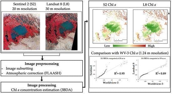
Quantitative evaluation of four semi-empirical algorithms for estimating Chl a from L8 and S2 imagery;
(2)
Evaluation of the performance of L8 and S2 sensors for Chl a mapping in LC using the algorithms;
(3)
Validation of derived Chl a estimates in comparison with higher resolution image sources in the LC area.
For this study, we used S2 and L8 images to estimate Chl a concentrations at 10-, 20- and 30-m resolutions. Using estimates from WV3, we statistically evaluated the Chl a mapped from S2 and L8 images. The most appropriate spectral bands which could be used to map out Chl a for this area were also identified through performance evaluations. Although the term “validation” is used here for the derived Chl a, no ground observations of Chl a were available. Instead, the validation process involved comparisons to equivalent measurements from significantly higher resolution WorldView products.

2. Materials and Methods

2.1. Overview of the Study Area

As illustrated in Figure 1, LC is situated on the boundary between CMR, Niger (NER), Nigeria (NGA) and TCD. Approximately 90% of LC’s freshwater is supplied by the Chari-Logone River, which flows into LC from the southern section of the lake. The Yobe River supplies approximately 3% of the water that makes up the lake. The water mostly comes in from the north towards NGA and is highly dependent on the rainy season [47]. Between 1973 and 1975, Lake Chad lost approximately 90% (from 24,000 to 1700 km2) of its surface water. Studies have found that this decrease in water level was due to anthropogenic activities and severe droughts within that period [43,48,49]. The population around this water resource is expected to double by 2050; consequently, the demand on the lake surface water with respect to the daily and economic activities of its community is anticipated to increase [50]. Following its surface water decline, few studies have focused on the associated water quality changes at a large temporal and spatial scale. The southern pool of Lake Chad, which carries more than 70% of the surface water, is our region of interest (Figure 1).

2.2. Materials

2.2.1. Sentinel-2

The launch of S2 satellites, which supply multispectral images, created viable datasets for monitoring the quality of a water body. The onboard Multispectral Instrument (MSI) with a high 12-bit radiometric resolution generates spectral images with 13 bands of varying wavelengths (Table 1). Images from the MSI sensor have a wide spatial and temporal resolution, and a wide field of view (FoV). These images also have a high signal-to-noise ratio (SNR). These advantages explain why researchers have monitored lakes and rivers using these images [51,52,53]. We downloaded the S2 image which correspond to the top of atmosphere (ToA) product from the European state agency website (https://scihub.copernicus.eu/). The image had less than 10% cloud coverage.

2.2.2. Landsat

The L8 satellite supplies multispectral images comprising of 11 bands, the majority of which have a 30-m spatial resolution. The red, near-infrared (NIR) and shortwave infrared (SWIR) bands in the L8 satellite images have a narrower bandwidth than those from previous Landsat missions. The L8 radiation resolution was increased to 16 bits, and the SNR was increased significantly. These advances improved L8′s pigment discrimination ability. Though built for terrestrial applications, these bands have proven useful for estimating concentrations of Chl a in water bodies [54,55]. In this study, we selected available OLI/L8 images with no cloud cover. The image can be found in path 185, row 51.

2.2.3. WorldView-3

WorldView-3 (WV3) sensors produce super-spectral and very-high-resolution imagery, comprising of panchromatic, multispectral and SWIR bands. The sensors have eight multispectral (1.24-m resolution) bands, from Coastal to NIR-2 (Table 1). WV3 was selected to develop both training and validation datasets, and served as a comparison dataset for S2 and L8 (Table 2). The WV3 image that was used in this study covered an area of approximately 50 square kilometers, and was acquired with a total cloud cover of 1%. For this area, the average price of an image representing a square kilometer of land is approximately USD 30. Images from WV3 can be purchased from www.digitalglobe.com.
The data acquisition dates in Table 2 show an interval of several days between the sensors used in this study. This could be a potential source of error when carrying out a comparison across sensors. Although inter-sensor comparison was not the main objective of this study, certain measures were taken into consideration before these datasets were acquired. These include the following: (i) Visual inspection of all WV-3 images available for the month of December 2015 on the DigitalGlobe website was carried out, and revealed no abrupt surface water changes which could ultimately alter the water quality in this area. (ii) The LCB official website reported no significant flooding event during this study period. (iii) Near-cloud-free Sentinel-2A and Landsat-8 images were acquired within four days for processing. This reduced the impact of any surface water changes between the sensors.

2.3. Methods

2.3.1. Satellite Data Preprocessing

When radiation travels from a reflected surface through the atmosphere to a satellite sensor, absorption and scattering from different molecules modifies the direction and intensity of the emitted radiation. The SNR ratio of the ToA radiance of a waterbody varies depending on the atmospheric aerosol concentrations. This makes controlling these atmospheric effects a major challenge when dealing with remote sensing of inland water bodies. An accurate estimation of any water quality parameter requires atmospheric correction (AC) for any given atmospheric effects [56]. As such, before image processing in this study, rigorous AC was conducted across all the images. To achieve uniformity in the processing steps, all the images used in this study were Level 1 products.
Because we will be estimating Chl a concentrations from satellite imagery without reference to in situ estimates, it is essential to remove any intervening atmospheric effects from the acquired Sentinel and Landsat images. This reduces error sources from the resulting estimated Chl a concentrations in the lake. For this purpose, two conventional AC algorithms were applied: Fast Line-of-Sight Atmospheric Analysis of Hypercubes (FLAASH) [57] and Quick Atmospheric Correction (QUAC) [58]. The FLAASH method is used to estimate the scattering effects caused by the atmosphere. FLAASH needs additional input from each image in order to operate. These specific inputs are found in header files which are usually downloaded alongside their respective multispectral images. The QUAC is a simpler method which establishes a relationship between the surface reflectance and the observed radiance signal. QUAC can be applied to VIS and NIR-SWIR bands, and does not require additional inputs from image header files. FLAASH and QUAC can be conducted using the built-in functions in ENVI®.
The downloaded S2 satellite images (L1C) included previously-orthorectified ToA images. Using the two AC methods (FLAASH and QUAC), we processed the acquired L1C images and obtained bottom-of-atmosphere (BoA) 2A-level products. Similar ACs were performed for L8 images, whereby their digital numbers (DNs) were converted to sensor radiance values. The radiance values were then converted to bottom surface reflectance, which represents surface reflectance from the water body. WV3 spectral imagery was used as a reference to evaluate which AC methods performed most accurately for both Sentinel and Landsat sensors. For this purpose, 40 sampling points were randomly selected directly over the water surface feature from the WV-3 image. From visual inspection, no significant changes were registered within or around the selected 40 sampling points. The same sampling points were used to retrieve reflectance values from the S2 and L8 images for comparison. Since the S2 and L8 spatial resolutions vary with bands, the WV-3 product was resampled using the nearest neighbor method to match their respective band resolutions before comparison. For a more accurate atmospheric correction comparison across sensor images, it is advisable to acquire the images on the same date, or as close to the same date as possible. The average root mean square percentage (RMS (%)), defined in equation 1, was used to assess this preprocessing step.
Average   RMS ( % ) = 100 × i n ( R i ( WV 3 ) R i ( image ) ) 2   i n ( R i ( image ) ) 2  
where R (WV3) is the referenced WV3 surface reflectance, and R (image) is the surface reflectance of the S2 and L8 images for a unique band at sampling point i. We recorded n = 40 sampling points (n = 40). These inputs were used to compute the average root mean square percentage for specific bands.

2.3.2. Estimating Chl a Concentration

Research studies have shown that atmospheric and aerosol effects on satellite products can be reduced using spectral ratios. These spectral ratios have also been frequently used to estimate Chl a [56,59]. Chl a is known to have prominent scattering–absorption patterns between certain wavelengths. For instance, around the blue region of the electromagnetic (em) spectrum (between 450 and 475 nm), Chl a exhibits high absorption tendencies. This is also experienced around the red region at 670 nm. At the green and NIR regions of the em spectrum, Chl a exhibits high reflectance values that could reach 500 and 700 nm, respectively. This information has extensively been used by researchers to develop Chl a quantification algorithms [31,51].
Numerous water quality satellite reflectance algorithms have been used for retrieving Chl a concentration [59,60]. In this study, we selected four algorithms: 2BDA [27,61], 3BDA [28,62], NDCI [22] and FLH [29]. These algorithms were selected based on reviews and the Chl a estimation accuracy for lakes [63,64]. These accuracies relied on the degree of agreement between derived Chl a estimates from satellite images, and Chl a estimates obtained on site and tested using laboratory methodologies. Band position, spacing and width were also considered while selecting the four algorithms for this study. Another selection criterion was the ease with which these algorithms could be implemented by resource managers in the future
Using the Band Math function in ENVI®, we first established the performance baseline for this study by applying 2BDA, 3BDA, NDCI and FLH algorithms to an atmospherically corrected WV3 reflectance image. The same algorithms were then applied to Sentinel-2 and L8 reflectance products (Table 3). Band Resampling was performed before processing the S2 image using 2BDA, 3BDA and NDCI index, as shown in Table 3. S2 Band 4 (10-m resolution) was resampled to match the resolutions of bands 5 and 8b (20-m) using the nearest neighbor method, which is an easy-to-compute resampling method that preserves the input data values during processing. The resulting S2 2BDA, 3BDA and NDCI index products had a 20-m resolution, while that for FLH was maintained at its original 10-m resolution.

2.3.3. Accuracy

The accuracies of modeled Chl a data from S2 and L8 images, and comparisons between them, were evaluated using data developed from WV3. For this study, we are interested in quantifying Chl a concentrations from S2 and L8 images (Figure 2). Accordingly, water pixels from the WV3 images were extracted for all the bands. This was followed by manually removing uncertain classes, which appeared predominantly around the boundary edges. The obtained water pixels were upscaled to 10-, 20- and 30-m resolutions using an area-weighted spatial model. The model simply averages neighboring smaller pixels into large ones. Consequently, the WV3 pixels could represent the percentage of Chl a concentrations at scales that matched the Landsat and Sentinel images. The algorithms in Table 3 were subsequently applied to the surface reflectance from the WV3 image.
From the newly derived Chl a data, we randomly selected training and validation datasets for the 10-, 20- and 30-m spatial resolution images. These datasets were sampled equally across the test site to ensure the representation of the entire range of Chl a. The training and validation sampling points were used to map Chl a across the S2 and L8 images. The S2 and L8 images were also resampled from the training and validation datasets so that their sampling points and grids would overlap at exactly 10 and 20 m for S2, and 30 m for L8 pixels.
After applying the Chl a extraction algorithm to the surface reflectance of the S2 and L8 images, their respective resulting indexed products were used as variables for Chl a mapping comparison. The evaluation of the derived Chl a estimates was carried out using similar estimates derived from the WV3 images. The root mean square error (RMSE) and relative area error (RAE) were used as the statistical metric for this evaluation purpose. They can be calculated using the following formula:
RMSE = i 1 n ( X o b s , i X m o d , i ) 2   n
RAE = i = 1 n A o b s , i i = 1 n A m o d , i i = 1 n A o b s , i
where Xobs,i is the referenced chlorophyll concentration at point i, Xmod,i is the modeled estimate of Chl a concentration at point i, n represents the total number of validation points, and Aobs,i and Amod,i represent areas of the referenced and modeled Chl a estimates for point i.

3. Results

3.1. Atmospheric Correction Evaluation

The European Space Agency (ESA) and the United States Geological Survey (USGS) primarily distribute uncorrected ToA reflectance or radiance products. As recommended, users typically perform AC to convert the DNs from the satellite imagery into BoA reflectance, before conducting analyses on any of the satellite products.
A statistical analysis illustrates that the AC algorithms used for this case offer similar performances across a subset of the spectral bands (Figure 3a). The RMS was plotted to select the highest-performing algorithm. FLAASH and QUAC produced RMS values of approximately 11% and 14%, respectively, for the S2 bands. FLAASH produced the most accurate AC results. The Chl a estimation algorithms shown in in Table 3 were applied to the S2A images, which were atmospherically corrected by the FLAASH method.
Averaged over the seven Landsat bands, FLAASH and QUAC produced average RMS values of 13% and 15%, respectively. Both yielded reasonable results, with abnormalities occurring in the sixth and seventh bands of the FLAASH and QUAC atmospheric results (Figure 3b). Of the two algorithms, FLAASH produced the most accurate AC results for our Landsat image. The Chl a estimation algorithms in Table 3 were performed using Landsat imagery atmospherically corrected using FLAASH.

3.2. Analysis of Chl a Concentration

3.2.1. Chl a Estimation Algorithm Evaluation

For evaluating the performances of the 2BDA, 3BDA, NDCI and FLH algorithms in extracting estimates of Chl a concentrations in Lake Chad, we first applied each algorithm to 1.8-m resolution WV3 imagery. This enabled us to build a baseline product for evaluating Chl a estimates derived from Sentinel (10- and 20-m resolutions) and L8 (30-m resolution) images using the same algorithms. The 3BDA, NDCI and FLH algorithms performed accurately for both sensor images. Scatterplots between the referenced WV3 Chl a estimates and the modeled Chl a estimates from S2 and L8, for each Chl a estimation algorithm, are shown in the following sections. The 3BDA algorithm most accurately estimated Chl a from the S2 and L8 images. The FLH algorithm developed for Landsat-8 was also highly accurate.

3.2.2. Sentinel-2

All four algorithms demonstrated acceptable performance with the sentinel images used in this study. They had an average R2 value of 0.74, exhibiting adequate portability when compared to the outputs from the WV3 imagery (Figure 4). The 3BDA performed most accurately in this experiment, and was thus used to represent the results in this section (Figure 5). The FLH algorithm, which was developed for the L8 images, showed satisfactory performance (R2 = 0.6) in estimating Chl a from the S2 image. It was slightly below that of the 2BDA and NDCI. The statistical standard used to analyze the performance of retrieved Chl a data derived from the 2BDA, 3BDA, NDCI and FLH algorithms is depicted in Table 4.

3.2.3. Landsat

The algorithms (2BDA, 3BDA, NDCI and FLH) used to estimate Chl a concentrations with the L8 image were compared with the baseline estimates for the WV3 image. With respect to the L8 image, the results from the algorithms had a significant correlation with the estimated Chl a concentrations from WV3 (Figure 6). These algorithms had an average R2 of approximately 0.78. When compared to the algorithms used in this study, 3BDA, depicted in Figure 7, performed more accurately in extracting Chl a from the L8 image. The statistical standard used to analyze the 2BDA, 3BDA, NDCI and FLH algorithms’ performances in retrieving Chl a estimates from the L8 image is depicted in Table 4. Based on the disparity between Figure 5 and Figure 7, we note that the mapping of Chl a concentrations from the S2 and L8 images of Lake Chad is highly dependent on the type of Chl a extraction algorithm used.

4. Discussion

Chl a concentrations move vertically along the water column, and are variable in time and space. Such vertical movements usually result in a patchy spatial distribution of Chl a, which might develop in only a few hours [13]. Detecting Chl a changes and movements using in situ measurements is challenging, especially for an area with a limited in situ monitoring infrastructure. Therefore, Chl a estimates from satellite multispectral and hyperspectral imagery can complement routine sampling in the Lake Chad area [35]. Given the lack of in situ Chl a measurement, WV3 imagery was used as a baseline to study the performances of estimations of Chl a from S2 and L8 images, using the 2BDA, 3BDA, NDCI and FLH algorithms.

4.1. Performance of Chl a Estimation from Sentinel-2

S2 data, obtained from recently launched operational Sentinel satellites, have been used alongside algorithms, and evaluated for water quality analysis. Amongst the algorithms used on the S2 images, numerous algorithms specific to Chl a estimation have been applied to S2 images in order to map out Chl a concentrations in lakes and rivers [33,34,35]. In this study, the 2BDA (R2 = 0.6), 3BDA (R2 = 0.9) and NDCI (R2 = 0.7) accurately estimated Chl a concentrations within the Lake Chad Basin (Figure 5). These outcomes are encouraging for Lake Chad, since these S2 image and Chl a extraction algorithm pairs provide resource managers with options for detecting and monitoring harmful algal blooms (HABs) for this area. The three algorithms had an average R2 of approximately 0.7, indicative of a high potential with regard to detecting and estimating Chl a in Lake Chad. Despite high correlation, visual inspection revealed that the 2BDA algorithm overestimated Chl a concentration. The 3BDA exhibited the best performance in terms of Chl a estimation accuracy. It had an R2 of 0.95, with an RMSE of 2.8% (Table 4). The good performance of 3BDA has been previously demonstrated in similar studies that evaluated the performance of the 3BDA model and yielded high-quality results [16,33]. Figure 8 shows the Chl a concentration patterns derived from S2 using 3BDA for our study site. At the center of the lake, the Chl a concentration is stable. However, moving outward away from the lake’s center, the Chl a concentration increases.
The correlation results obtained from this study indicate that Chl a concentrations can be estimated in the Lake Chad area using a combination of red-edge, red and NIR bands from S2 imagery. This is also backed by the performances of Chl a estimation algorithms, which had similar band combinations (NDCI). Furthermore, given the dual collection of S2 images, along with their characteristic wide swaths, S2 satellites present a unique opportunity, and offer a set of free products in a timely manner (~5–10 days) to water quality managers in Lake Chad. Due to its high correlation performance, we suggest that the 3BDA algorithm could be used alongside S2 images as a tool for monitoring and estimating Chl a concentrations in the Lake Chad area.

4.2. Performance of Chl a Estimation from Landsat 8

The size of Lake Chad (approximately 1700 km2) supports the use of using L8 images (30-m resolution) for its monitoring. Monitoring and estimating in small reservoirs can be hindered by adjacency effects [34]. Almost all the tested algorithms performed accurately in depicting Chl a estimations and mapping in Lake Chad. The performance evaluation confirmed that the most appropriate Chl a algorithms for L8, with regard to the estimation of Chl a, were 3BDA and NDCI. Both algorithms predominantly consisted of the red and near infrared (NIR) bands (Table 4). Although the evaluation of the 2BDA algorithm was acceptable (R2 of 0.7), the results obtained showed an overestimation of Chl a concentrations. Other studies have also demonstrated the poor performance of the 2BDA algorithm in estimating Chl a concentrations, and attributed such poor performance to the narrow width and position of the Landsat-8 NIR band [17,28]. Furthermore, the NIR band has an average wavelength of 865 nm, which is greater than the Chl a absorbance peak (~700 nm).
The correlation results obtained from this study indicate that Chl a concentrations can be estimated in the Lake Chad area using a combination of the blue-green, red and NIR bands from the L8 images. Consider the higher performance of 3BDA (R2 of 0.89, RMSE of 5.1%) for the L8 image, which was developed using the blue, green and red L8 bands (Table 3). Figure 9 show the Chl a concentration pattern derived from L8 using 3BDA for the southern pool of Lake Chad. Similar to the S2 result shown in Figure 8, the Chl a concentration at the center of the lake seems to be stable. However, moving outward away from the lake’s center, the Chl a concentration increases.
NDCI, which is characterized by a red-NIR band combination and is extensively used for Chl a monitoring, had an R2 of 0.75. This was slightly greater than that of the FLH (R2 of 0.73) algorithm, which was the third-highest result with regard to Chl a estimation amongst the four algorithms. This FLH algorithm measures the green peak’s height relative to that of the red and violet minima within the bands. Given the high-quality performance of the 3BDA algorithm, we suggest that this algorithm could be used alongside L8 images as a tool for monitoring and estimating Chl a concentration in the Lake Chad area.
Overall, the results of this performance study from the MSI and OLI sensors are favorable, but there are limitations. Satellites are known to have low SNR ratios over water bodies. This is because most of these satellites were developed for application in terrestrial environments. However, following rigorous validation practices, researchers have agreed that terrestrial satellites can be applied in inland aquatic studies [16,28,33]. Furthermore, for comparison with data products from different sensors, differing data acquisition dates from the sensors could also be a source of error. For instance, besides achieving good performance during the preprocessing (atmospheric correction) and processing (Chl a estimation) phases, it is important to make sure the data acquisition dates are closer to each other. In doing so, the effect of time-dependency is reduced.
L8 has a repeat cycle of 16 days, as opposed to that of S2, which is 10 days. However, combining products from the two S2 satellites (S2A since 2015, and S2B since 2017) further reduces the repeat cycle to 5 days. Consequently, when products from the L8 and S2 are combined, their revisit time is estimated to be ~2.9 days. The temporal and spatial resolution of these satellites (10 and 20 m for S2 MSI, and 30 m for L8 OLI) provides a variety of datasets needed for water quality monitoring in lakes. It also enables the capture of much smaller waterbodies. A future study combining the data products provided by S2 and L8, alongside an appropriate water quality estimation algorithm, could create a new and more reliable means of quantifying Chl a changes at a higher temporal resolution. Authors should also consider understanding the varying performances between the algorithms and image pairs. Given the unconstrained error sources in this study, it is important to note that the derived Chl a concentration values in Figure 8 and Figure 9 are included for visual inspection, and do not serve as a metric of comparison between the sensor images. Another possible future study could carry out a statistical comparison of 3BDA-derived Chl a estimates from S2 and L8 at the same resolution. Nonetheless, from visual inspection, it is clear that a strong correlative relationship exists between the 3BDA-derived Chl a patterns from the S2 and L8 images, despite their varying resolutions of 20 m and 30 m, respectively (Figure 8 and Figure 9). The incremental increase in Chl a concentration moving away from Lake Chad’s center is probably due to the shallow water depths and high human interaction around those areas.
This paper offers satellite sensors and algorithm pair options to assist environmental managers. It demonstrates the ability of S2 and L8 images to provide estimated Chl a concentration using appropriate Chl a retrieval algorithms. This was performed in this study using Chl a estimation algorithms, and using their respective RMSE to identify which had the best performance for this area. (Table 4, Figure 4 and Figure 6). Although the S2 MSI sensor is similar to the L8 OLI sensor, S2 has a slight advantage over L8. S2 has a greater revisit period, and its products contain more bands in the visible and near infrared wavelengths. S2 also has a lower SNR compared to OLI, and the positions and widths of their bands differs as well. This does not indicate a more effective retrieval of Chl a concentrations for any or both of these sensors, but rather an evaluation of the performances of the Chl a estimation indexes from S2 (10- and 20-m resolution) and L8 (30-m resolution), vis-à-vis WV3 (1.24-m resolution) under similar conditions.

5. Conclusions

In this study, we investigated the potential applicability of S2 and L8 images for estimating Chl a concentrations in Lake Chad. To accomplish this, four water quality extraction algorithms, which have been frequently used and validated by researchers, were selected and applied to S2 and L8 images. This research used atmospherically corrected WV3, S2 and L8 images to evaluate the performances and relative applicability of 2BDA, 3BDA, NDCI and FLH Chl a algorithms in Lake Chad.
The AC of satellite imagery is vital in order to eliminate atmospheric or aerosol effects from the satellite images before processing. We evaluated two AC processors: FLAASH and QUAC. Performing statistical analysis on 40 sampling points within the test site, FLAASH was selected as the AC processor for the Sentinel and Landsat images. FLAASH was chosen due to its low average RMS values (11.2% for Sentinel and 13.1% for Landsat) at bands useful for deriving Chl a. Estimating the Chl a concentrations from S2 and L8 images in Lake Chad involved four steps: (1) converting the L8 bands’ DNs to absolute ToA reflectance, and scaling the ToA reflectance of the S2 bands; (2) converting the ToA to surface reflectance, which signifies surface reflectance originating from the lake’s surface; (3) converting the lake’s surface reflectance to remote sensing reflectance (Rrs); and (4) estimating Chl a from the Rrs using 2BDA, 3BDA, NDCI and FLH algorithms.
The algorithm evaluation indicated efficiency in the applicability of the 3BDA and NDCI algorithms. Correlation analysis showed that 3BDA can be used to estimate Chl a concentration in the southern pool of Lake Chad. The spatial distributions of Chl a, derived from the S2 and L8 images, represented the Chl a concentrations in our study areas (Figure 8 and Figure 9). This analysis confirms the need for further validation analysis between the sensor images in order to improve their performances in estimating Chl a concentrations using water quality algorithms. Furthermore, the need for improved bio-optical algorithms is confirmed for this study region. Accordingly, the obtained findings demonstrate the potential applicability of the S2 and L8 imagery as valuable data sources for mapping Chl a concentrations in the Lake Chad area.

Author Contributions

Conceptualization, W.G.B. and S.-I.L.; Funding acquisition, S.-I.L.; Investigation, W.G.B. and S.-I.L.; Methodology, W.G.B.; Project administration, W.G.B. and S.-I.L.; Validation, W.G.B.; Visualization, W.G.B.; Writing—original draft, W.G.B.; Writing—review and editing, S.-I.L. All authors have read and agreed to the published version of the manuscript.

Funding

This research supported by Basic Science Research Program through the National Research Foundation of Korea (NRF) funded by the ministry grant (NRF-2018R1D1A1A09083120).

Acknowledgments

The authors would like to thank the reviewers and editors for their valuable comments and suggestions.

Conflicts of Interest

The authors declare no conflict of interest. The funders had no role in the design of the study; in the collection, analyses, or interpretation of data; in the writing of the manuscript, or in the decision to publish the results.

References

  1. Robert, E.; Harvey, A.; Eric, O. Drought African lake management initiatives: The global connection. Lakes Reserv. Res. Manag. 2006, 11, 203–213. [Google Scholar] [CrossRef]
  2. Dube, T.; Mutanga, O.; Seutloali, K.; Adelabu, S.; Shoko, C. Water quality monitoring in sub-Saharan African lakes: A review of remote sensing applications. Afr. J. Aquat. Sci. 2015, 40, 1–7. [Google Scholar] [CrossRef]
  3. Wenbin, Z.; Shaofeng, J.; Upmanu, L.; Qing, C.; Rashid, M. Relative contribution of climate variability and human activities on the water loss of the Chari/Logone River discharge into Lake Chad: A conceptual and statistical approach. J. Hydrol. 2019, 569, 519–531. [Google Scholar] [CrossRef]
  4. Alla, S.; Jejung, L.; Hahn, C.J.; John, B.; John, L.; Frederick, S.; Ibrahim, B.; Guillaume, F.; Soma, S.; Charles, M. Application of GRACE to the estimation of groundwater storage change in a data-poor region: A case study of Ngadda catchment in the Lake Chad Basin. Hydrol. Process. 2019, 34, 941–955. [Google Scholar] [CrossRef]
  5. Buma, W.G.; Lee, S.I.; Seo, J.Y. Recent surface water extent of Lake Chad from multispectral sensors and grace. Sensors 2018, 18, 2082. [Google Scholar] [CrossRef] [Green Version]
  6. Koponen, S.; Pullainen, J.; Kallio, K.; Hallikainen, M. Lake water quality classification with airborne hyperspectral spectrometer and simulated MERIS data. Remote Sens. Environ. 2002, 79, 51–59. [Google Scholar] [CrossRef]
  7. Duan, H.; Zhang, Y.; Zhang, B.; Song, K.; Wang, Z. Assessment of chlorophyll-a concentration and trophic state for Lake Chagan using Landsat TM and field spectral data. Environ. Monit. Assess. 2007, 129, 295–308. [Google Scholar] [CrossRef]
  8. Wozniak, M.; Bradtke, K.M.; Krezel, A. Comparison of satellite chlorophyll a algorithms for the Baltic Sea. J. Appl. Remote Sens. 2014, 8, 083605. [Google Scholar] [CrossRef] [Green Version]
  9. Salem, S.I.; Higa, H.; Kim, H.; Kobayashi, H.; Oki, K.; Oki, T. Assessment of chlorophyll-a algorithms considering different trophic statuses and optimal bands. Sensors 2017, 17, 1746. [Google Scholar] [CrossRef] [Green Version]
  10. Carstensen, J.; Klais, R.; Cloern, J.E. Phytoplankton blooms in estuarine and coastal waters: Seasonal patterns and key species. Estuar. Coast. Shelf Sci. 2015, 162, 98–109. [Google Scholar] [CrossRef] [Green Version]
  11. Zhang, F.; Li, J.; Shen, Q.; Zhang, B.; Wu, C.; Wu, Y.; Wang, G.; Wang, S.; Lu, Z. Algorithms and schemes for chlorophyll a estimation by remote sensing and optical classification for turbid lake Taihu, China. IEEE J. Sel. Top. Appl. Earth Obs. Remote Sens. 2015, 8, 350–364. [Google Scholar] [CrossRef]
  12. Crétaux, J.F.; Jelinski, W.; Calmant, S.; Kouraev, A.; Vuglinski, V.; Bergé-Nguyen, M.; Gennero, M.-C.; Nino, F.; Del Rio Abarca, R.; Cazenave, A.; et al. SOLS: A lake database to monitor in the Near Real Time water level and storage variations from remote sensing data. Adv. Space Res. 2011, 47, 1497–1507. [Google Scholar] [CrossRef]
  13. Agha, R.; Cires, S.; Wörmer, L.; Domínguez, J.A.; Quesada, A. Multi-scale strategies for the monitoring of fresh-water cyanobacteria: Reducing the sources of uncertainty. Water Res. 2012, 46, 3043–3053. [Google Scholar] [CrossRef] [PubMed]
  14. Andres, L.; Boateng, K.; Borja-Vega, C.; Thomas, E. A review of in situ and remote sensing technologies to monitor water and sanitation interventions. Water 2018, 10, 756. [Google Scholar] [CrossRef] [Green Version]
  15. Kogan, F.N. Application of vegetation index and brightness temperature for drought detection. Adv. Space Res. 1995, 15, 91–100. [Google Scholar] [CrossRef]
  16. Toming, K.; Kutser, T.; Laas, A.; Sepp, M.; Paavel, B.; Nõges, T. First experiences in mapping lake water quality parameters with Sentinel-2 MSI imagery. Remote Sens. 2016, 8, 640. [Google Scholar] [CrossRef] [Green Version]
  17. Mishra, S.; Mishra, D.R. Normalized difference chlorophyll index: A novel model for remote estimation of chlorophyll-a concentration in turbid productive waters. Remote Sens. Environ. 2012, 117, 394–406. [Google Scholar] [CrossRef]
  18. Boucher, J.; Weathers, K.C.; Norouzi, H.; Steele, B. Assessing the effectiveness of Landsat 8 chlorophyll-a retrieval algorithms for regional freshwater monitoring. Ecol. Appl. 2018, 28, 1044–1054. [Google Scholar] [CrossRef] [Green Version]
  19. Gower, J.; King, S.; Borstad, G.; Brown, L. Detection of intense plankton blooms using the 709 nm band of the MERIS imaging spectrometer. Int. J. Remote Sens. 2005, 26, 2005–2012. [Google Scholar] [CrossRef]
  20. Gong, G.-C.; Wen, Y.-H.; Wang, B.-W.; Liu, G.-J. Seasonal variation of chlorophyll a concentration, primary production and environmental conditions in the subtropical East China Sea. Deep Sea Res. Part II Top. Stud. Oceanogr. 2003, 50, 1219–1236. [Google Scholar] [CrossRef]
  21. Hu, C. A novel ocean color index to detect floating algae in the global oceans. Remote Sens. Environ. 2009, 113, 2118–2129. [Google Scholar] [CrossRef]
  22. Shahzad, M.I.; Meraj, M.; Nazeer, M.; Zia, I.; Inam, A.; Mehmood, K.; Zafar, H. Empirical estimation of suspended solids concentration in the Indus Delta Region using Landsat-7 ETM+ imagery. J. Environ. Manag. 2018, 209, 254–261. [Google Scholar] [CrossRef] [PubMed]
  23. Huang, C.; Li, Y.; Yang, H.; Sun, D.; Yu, Z.; Zhang, Z.; Chen, X.; Xu, L. Detection of algal bloom and factors influencing its formation in Taihu Lake from 2000 to 2011 by MODIS. Environ. Earth Sci. 2014, 71, 3705–3714. [Google Scholar] [CrossRef]
  24. Zhou, B.; Shang, M.; Wang, G.; Zhang, S.; Feng, L.; Liu, X.; Wu, L.; Shan, K. Distinguishing two phenotypes of blooms using the normalised difference peak-valley index (NDPI) and Cyano-Chlorophyta index (CCI). Sci. Total Environ. 2018, 628, 848–857. [Google Scholar] [CrossRef] [PubMed]
  25. Mishra, D.R.; Schaeffer, B.A.; Keith, D. Performance evaluation of normalized difference chlorophyll index in northern Gulf of Mexico estuaries using the Hyperspectral Imager for the Coastal Ocean. GISci. Remote Sens. 2014, 51, 175–198. [Google Scholar] [CrossRef]
  26. Toming, K.; Kutser, T.; Uiboupin, R.; Arikas, A.; Vahter, K.; Paavel, B. Mapping water quality parameters with sentinel-3 ocean and land colour instrument imagery in the Baltic Sea. Remote Sens. 2017, 9, 1070. [Google Scholar] [CrossRef] [Green Version]
  27. Watanabe, F.; Alcantara, E.; Rodrigues, T.; Rotta, L.; Bernardo, N.; Imai, N. Remote sensing of the chlorophyll a based on OLI/Landsat-8 and MSI/Sentinel-2A (Barra Bonita reservoir, Brazil). An. Acad. Bras. Ciênc. 2018, 90, 1987–2000. [Google Scholar] [CrossRef] [Green Version]
  28. Abdelmalik, K. Role of statistical remote sensing for Inland water quality parameters prediction. Egypt. J. Remote Sens. Space Sci. 2018, 21, 193–200. [Google Scholar] [CrossRef]
  29. Zhao, D.Z.; Xing, X.G.; Liu, Y.G.; Yang, J.H.; Wang, L. The relation of chlorophylla concentration with the reflectance peak near 700 nm in algae-dominated waters and sensitivity of fluorescence algorithms for detecting algal bloom. Int. J Remote Sens. 2010, 31, 39–48. [Google Scholar] [CrossRef]
  30. Alawadi, F. Detection of surface algal blooms using the newly developed algorithm surface algal bloom index (SABI). Remote Sens. Ocean Sea Ice Large Water Reg. 2010, 7825, 7782506. [Google Scholar] [CrossRef] [Green Version]
  31. Beck, R.A.; Zhan, S.; Liu, H.; Tong, S.T.Y.; Yang, B.; Xu, M.; Ye, Z.; Huang, Y.; Shu, S.; Wu, Q.; et al. Comparison of satellite reflectance algorithms for estimating chlorophyll-a in a temperate reservoir using coincident hyperspectral aircraft imagery and dense coincident surface observations. Remote Sens. Environ. 2016, 178, 15–30. [Google Scholar] [CrossRef] [Green Version]
  32. Zhou, L.; Xu, B.; Ma, W.; Zhao, B.; Li, L.; Huai, H. Evaluation of Hyperspectral Multi-Band Indices to Estimate Chlorophyll-A Concentration Using Field Spectral Measurements and Satellite Data in Dianshan Lake, China. Water 2013, 5, 525–539. [Google Scholar] [CrossRef]
  33. Bresciani, M.; Cazzaniga, I.; Austoni, M.; Sforzi, T.; Buzzi, F.; Morabito, G.; Giardino, C. Mapping phytoplankton blooms in deep subalpine lakes from Sentinel-2A and Landsat-8 M. Hydrobiologia 2018, 824, 197–214. [Google Scholar] [CrossRef] [Green Version]
  34. Pereira-Sandoval, M.; Urrego, P.; Ruiz-Verdú, A.; Tenjo, C.; Delegido, J.; Soria-Perpinyà, X.; Vicente, E.; Soria, J.; Moreno, J. Calibration and validation of algorithms for the estimation of chlorophyll-a concentration and Secchi depth in inland waters with Sentinel-2. Limnetica 2019, 38, 471–487. [Google Scholar]
  35. Anster, A.; Alikas, K. Retrieval of Chlorophyll a from Sentinel-2 MSI Data for the European Union Water Framework Directive Reporting Purposes. Remote Sens. 2019, 11, 64. [Google Scholar] [CrossRef] [Green Version]
  36. Luxereau, A.; Genthon, P.; Karimou, A. Fluctuations in the size of Lake Chad: Consequences on the livelihoods of the riverain peoples in eastern Niger. Reg. Environ. Chang. 2011, 12, 507–521. [Google Scholar] [CrossRef]
  37. Lemoalle, J.; Bader, J.-C.; Leblanc, M.; Sedick, A. Recent changes in Lake Chad: Observations, simulations and management options (1973–2011). Glob. Planet. Chang. 2012, 80–81, 247–254. [Google Scholar] [CrossRef]
  38. Boronina, A.; Ramillien, G. Application of AVGRR imagery and GRACE measurements for calculation of actual evapotranspiration over the Quaternary aquifer (Lake Chad basin) and validation of groundwater models. Hydrol. J. 2008, 348, 98–109. [Google Scholar] [CrossRef]
  39. Coe, M.T.; Birkett, C.M. Calculation of river discharge and prediction of lake height from satellite radar altimetry: Example for the Lake Chad basin. Water Resour. Res. 2004, 40, W10205. [Google Scholar] [CrossRef]
  40. Buma, W.G.; Lee, S.I.; Seo, J.Y. Hydrological evaluation of Lake Chad Basin using space borne and hydrological model observations. Water 2016, 8, 205. [Google Scholar] [CrossRef] [Green Version]
  41. Leblanc, M.; Razack, M.; Dagorne, D.; Mofor, L.; Jones, C. Application of Meteosat thermal data to map soil infiltrability in the central part of the Lake Chad basin, Africa. Geophys. Res. Lett. 2003, 30. [Google Scholar] [CrossRef]
  42. Leblanc, M.; Lemoalle, J.; Bader, J.-C.; Tweed, S.; Mofor, L. Thermal remote sensing of water under flooded vegetation: New observations of inundation patterns for the ‘Small’ Lake Chad. J. Hydrol. 2011, 404, 87–98. [Google Scholar] [CrossRef]
  43. Buma, W.G.; Lee, S.I. Multispectral Image-Based Estimation of Drought Patterns and Intensity around Lake Chad, Africa. Remote Sens. 2019, 11, 2534. [Google Scholar] [CrossRef] [Green Version]
  44. Benjamin, N.N.; Djoret, D. Nitrate pollution in groundwater in two selected areas from Cameroon and Chad in the Lake Chad basin. Water Policy 2010, 12, 722–733. [Google Scholar] [CrossRef]
  45. Vassolo, S.; Daïra, D. Water Quality in the Chadian Part of the Lake Chad Basin. Available online: https://www.bgr.bund.de/EN/Themen/Wasser/Projekte/abgeschlossen/TZ/Tschad/tschad-I_fb_en.html (accessed on 22 June 2020).
  46. Bello, M.; Ketchemen-Tandia, B.; Nlend, B.; Fouepe, A.; Fantong, W.Y.; Ngo, B.-N.; Garel, E.; Celle-Jeanton, H. Shallow groundwater quality evolution after 20 years of exploitation in the southern Lake Chad: Hydrochemistry and stable isotopes survey in the far north of Cameroon. Environ. Earth Sci. 2019, 78, 474. [Google Scholar] [CrossRef]
  47. Adeyeri, O.E.; Lamptey, B.L.; Lawin, A.E.; Sanda, I.S. Spatio-temporal precipitation trend and homogeneity analysis in Komadugu-Yobe basin, Lake Chad region. J. Climatol. Weather Forecast. 2017, 5, 12. [Google Scholar] [CrossRef]
  48. Lemoalle, J. Lake chad: A changing environment. In Dying and Dead Seas Climatic Versus Anthropic Causes; NATO Science Series: IV: Earth and Environmental Sciences; Nihoul, J.C.J., Zavialov, P.O., Micklin, P.P., Eds.; Springer: Dordrecht, The Netherlands, 2004; Volume 36. [Google Scholar] [CrossRef]
  49. Gao, H.; Bohn, T.J.; Podest, E.; McDonald, K.C.; Lettenmaier, D.P. On the causes of the shrinking of Lake Chad. Environ. Res. Lett. 2011, 6, 034021. [Google Scholar] [CrossRef] [Green Version]
  50. Lake Chad Basin Commission (LCBC). The Lake Chad Basin. 2014. Available online: http://www.cblt.org/en/lake-chad-basin (accessed on 17 June 2020).
  51. Tuuli, S.; Kristi, U.; Dainis, J.; Agris, B.; Matiss, Z.; Tiit, K. Validation and Comparison of Water Quality Products in Baltic Lakes Using Sentinel-2 MSI and Sentinel-3 OLCI Data. Sensors 2020, 20, 742. [Google Scholar] [CrossRef] [Green Version]
  52. Mohamed, E.; Ioannis, G.; Anas, O.; Jarbou, B.; Petros, G. Assessment of water quality parameters using temporal remote sensing spectral reflectance in arid environments, Saudi Arabia. Water 2019, 11, 556. [Google Scholar] [CrossRef] [Green Version]
  53. Katalin, B.; Károly, P.; Viktor, R.T.; Torbjørn, E. Remote sensing of water quality parameters over Lake Balaton by using sentinel-3 OLCI. Water 2018, 10, 1428. [Google Scholar] [CrossRef] [Green Version]
  54. Pahlevan, N.; Lee, Z.-P.; Wei, J.; Schaaf, C.B.; Schott, J.R.; Berk, A. On-orbit radiometric characterization of OLI (Landsat-8) for applications in aquatic remote sensing. Remote Sens. Environ. 2014, 154, 272–284. [Google Scholar] [CrossRef]
  55. Lobo, F.L.; Costa, A.P.F.; Novo, E.M.L.M. Time-series analysis of Landsat-MSS/TM/OLI images over Amazonian waters impacted by gold mining activities. Remote Sens. Environ. 2015, 157, 170–184. [Google Scholar] [CrossRef]
  56. Simon, N.T.; Tamlin, M.P.; Daniel, J.; Marc, S.; Matthew, R.V.R. Research trends in the use of remote sensing for inland water quality science: Moving towards multidisciplinary applications. Water 2019, 12, 169. [Google Scholar] [CrossRef] [Green Version]
  57. Anderson, G.P.; Felde, G.W.; Hoke, M.L.; Ratkowski, A.J.; Cooley, T.W.; James, H.; Chetwynd, J.; Gardner, J.A.; Adler-Golden, S.M.; Matthew, M.W.; et al. MODTRAN4-based atmospheric correction algorithm: FLAASH (fast line-of-sight atmospheric analysis of spectral hypercubes). Proc. SPIE-Int. Soc. Opt. Eng. 2002, 4725, 65–71. [Google Scholar] [CrossRef]
  58. Bernstein, L.S.; Lewis, P.E.; Adler-Golden, S.M.; Sundberg, R.L.; Levine, R.Y.; Perkins, T.C.; Berk, A.; Ratkowski, A.J.; Felde, G.; Hoke, M.L. Validation of the QUick atmospheric correction (QUAC) algorithm for VNIR-SWIR multi- and hyperspectral imagery. Proc. SPIE-Int. Soc. Opt. Eng. 2005, 5806, 668–678. [Google Scholar] [CrossRef]
  59. Mohammad, H.G.; Assefa, M.M.; Lakshmi, R. A Comprehensive Review on Water Quality Parameters Estimation Using Remote Sensing Techniques. Sensors 2016, 16, 1298. [Google Scholar] [CrossRef] [Green Version]
  60. Richard, J.; Richard, B.; Jakub, N.; Christopher, N.; Min, X.; Song, S.; Bo, Y.; Hongxing, L.; Erich, E.; Molly, R.; et al. Evaluating the portability of satellite derived chlorophyll-a algorithms for temperate inland lakes using airborne hyperspectral imagery and dense surface observations. Harmful Algae 2018, 76, 35–46. [Google Scholar] [CrossRef]
  61. Dall’Olmo, G.; Gitelson, A.A. Effect of bio-optical parameter variability on the remote estimation of chlorophyll-a concentration in turbid productive waters: Experimental results. Appl. Opt. 2005, 44, 412–422. [Google Scholar] [CrossRef] [Green Version]
  62. Gitelson, A.A.; Gritz, U.; Merzlyak, M.N. Relationships between leaf chlorophyll content and spectral reflectance and algorithms for non-destructive chlorophyll assessment in higher plant leaves. J. Plant Physiol. 2003, 160, 271–282. [Google Scholar] [CrossRef]
  63. Augusto-Silva, P.B.; Ogashawara, I.; Barbosa, C.C.F.; de Carvalho, L.A.S.; Jorge, D.S.F.; Fornari, C.I.; Stech, J.L. Analysis of MERIS reflectance algorithms for estimating chlorophyll-a concentration in a Brazilian Reservoir. Remote Sens. 2014, 6, 11689–117077. [Google Scholar] [CrossRef] [Green Version]
  64. Sauer, M.J.; Roesler, C.S.; Werdell, P.J.; Barnard, A. Under the hood of satellite empirical chlorophyll a algorithms: Revealing the dependencies of maximum band ratio algorithms on inherent optical properties. Opt. Express 2012, 20, 1–15. [Google Scholar] [CrossRef] [PubMed]
Figure 1. Study area. Image on the right represents water boundaries in the southern pool of Lake Chad which is the focus area in this study. Red square represents area where the performance evaluation of this study was carried out.
Remotesensing 12 02437 g001
Figure 2. Chl a estimation workflow using S2, L8 and WV3 images.
Remotesensing 12 02437 g002
Figure 3. Atmospheric correction analysis (RMS %) for each band (a) Sentinel and (b) Landsat image.
Remotesensing 12 02437 g003
Figure 4. Correlation between Sentinel Chl a concentration and Worldview at their respective spatial resolution (sr).
Remotesensing 12 02437 g004
Figure 5. Chl a extraction from S2 image image. (ac) index products were derived at 20-m spatial resolution while (d) was derived at 10-m spatial resolution. Increasing concentrations of Chl a are depicted by brighter pixels.
Remotesensing 12 02437 g005
Figure 6. Correlation between Landsat 8 Chl a concentration and Worldview at 30-m spatial resolution (sr).
Remotesensing 12 02437 g006
Figure 7. Chl a extraction from L8 image. All the index products were derived at 30-m spatial resolution. Increasing concentrations of Chl a are depicted by brighter pixels.
Remotesensing 12 02437 g007
Figure 8. Results of 3BDA Chl a concentration spatial pattern in the southern pool of Lake Chad from Sentinel-2 at 20-m spatial resolution. Increasing concentrations of Chl a are depicted by brighter pixels.
Remotesensing 12 02437 g008
Figure 9. Results of 3BDA Chl a concentration spatial pattern in the southern pool of Lake Chad from Landsat 8 at 30-m spatial resolution. Increasing concentrations of Chl a are depicted by brighter pixels.
Remotesensing 12 02437 g009
Table 1. Sensor band configurations used in this study.
SpectrumS2Range
(nm)
C
(nm)
SR
(m)
L8Range
(nm)
C
(nm)
SR
(m)
WV3Range
(nm)
C
(nm)
SR
(m)
AerosolB1433–45344360B1435–45144330B1400–4504251.24
BlueB2458–52349110B2452–51248030B2450–510480
GreenB3543–57856010B3533–59056130B3510–580545
Yellow--------B4585–625605
RedB4650–68066510B4636–67365430B5630–690660
RE-1B5698–71370520----B6705–745725
NIR-1B8b855–87586520B5851–87986530B7770–895832
* S2 = Sentinel-2, C = Center, SR= Spatial Resolution, L8 = Landsat 8, WV3 = Worldview-3.
Table 2. Description of S2, L8 and the reference WV3 scene.
Satellite DataReference Data
SensorDateSourceDate
OLI30 December 2015WorldView-322 December 2015
MSI26 December 2015
Table 3. Band Math for each algorithm used to derive Chl a concentration in Lake Chad.
Sensor ImageIndexBand Combination
Sentinel-22BDA(band5)/(band4)
3BDA(1/band4) − (1/(band5)) x (band8b)
NDCI(band5) − (band4)/(band5) + (band4)
FLH_violet(band3) − [(band4) + (band2) − (band4)]
Landsat 82BDA(band5)/(band4)
3BDA(band2) − (band4)/(band3)
NDCI(band5) − (band4)/(band5) + (band4)
FLH_violet(band3) − [(band4) + (band1) − (band4)]
WorldView-3 2BDA(band6)/(band5)
3BDA(1/(band5)) − (1/(band6) x (band7))
NDCI(band6) − (band5)/(band6) + (band5)
FLH_violet(band3) − [(band5) + ((band1) − (band5))]
Table 4. Statistical performances of Chl a estimation algorithms used in this study.
Algorithm Sentinel-2 Landsat 8
RMSERAERMSERAE
2BDA8.55.068.936.1
3BDA2.81.75.13.3
NDCI7.5 5.38.75.98
FLH violet9.046.684.3

