LiCSAR: An Automatic InSAR Tool for Measuring and Monitoring Tectonic and Volcanic Activity

Abstract

Space-borne Synthetic Aperture Radar (SAR) Interferometry (InSAR) is now a key geophysical tool for surface deformation studies. The European Commission’s Sentinel-1 Constellation began acquiring data systematically in late 2014. The data, which are free and open access, have global coverage at moderate resolution with a 6 or 12-day revisit, enabling researchers to investigate large-scale surface deformation systematically through time. However, full exploitation of the potential of Sentinel-1 requires specific processing approaches as well as the efficient use of modern computing and data storage facilities. Here we present Looking Into Continents from Space with Synthetic Aperture Radar (LiCSAR), an operational system built for large-scale interferometric processing of Sentinel-1 data. LiCSAR is designed to automatically produce geocoded wrapped and unwrapped interferograms and coherence estimates, for large regions, at 0.001° resolution (WGS-84 coordinate system). The products are continuously updated at a frequency depending on prioritised regions (monthly, weekly or live update strategy). The products are open and freely accessible and downloadable through an online portal. We describe the algorithms, processing, and storage solutions implemented in LiCSAR, and show several case studies that use LiCSAR products to measure tectonic and volcanic deformation. We aim to accelerate the uptake of InSAR data by researchers as well as non-expert users by mass producing interferograms and derived products.

1. Introduction

With the advent of the European Commission’s Copernicus two-satellite Sentinel-1 constellation, operated by the European Space Agency (ESA), a massive volume of high-quality C-band Synthetic Aperture Radar (SAR) observations with moderate spatial (2–14 m) and temporal resolution (6–12 days) has become freely available [1]. With a 250-km-wide cross-track coverage in the default Interferometric Wide Swath (IWS) mode, Sentinel-1 provides a unique and powerful dataset that has the potential to be used for monitoring surface deformation at spatial scales ranging from a few meters to tens of kilometers. Interferometric Synthetic Aperture Radar (InSAR) is a particularly suitable technique for measuring deformation induced by various geophysical phenomena, including the coseismic [2,3,4], postseismic [5,6,7,8] and interseismic phases of the earthquake deformation cycle [9,10,11,12], volcanic movements [13,14,15], terrain deformation due to geothermal activities [16,17,18] and slow-moving landslides [19,20]. Since the launch of Sentinel-1B in 2016, data are acquired globally with a typical revisit period of 12 days, and every 6 days in Europe [21]. The relatively short revisit time (compared to 35-days of previous ESA SAR satellites) is a significant advance because interferograms spanning a short interval usually maintain better coherence and allow a more accurate estimate of rapid deformation. The short revisit time also leads to a greater number of acquisitions, which is useful for statistical reduction of the noise contribution (e.g., due to atmospheric phase delay) in InSAR time series analyses [22]. The data is particularly important for global monitoring of tectonic and volcanic activities [23]. Over the last five years, numerous earthquakes and volcanic eruptions have already been imaged by Sentinel-1 interferograms, aiding rapid response and resulting in a greater scientific understanding of the events and their geophysical properties [8,24,25,26].

Despite the opportunities provided by the increasing availability of Sentinel-1 SAR data, it is still difficult to take full advantage of these resources, particularly for large-scale applications. Indeed, the full exploitation of the large amount of SAR data provided by the Sentinel-1 system, with its short revisit time and global-scale coverage (data are produced in the rate of ~13 TB/day), requires specific data preprocessing approaches (e.g., downsampling the SAR data—multilooking) or Big Data processing algorithms involving computer cluster facilities. The computing and storage demands require specific computing platforms [27]. Various research groups base their systematic processing approaches on open-source software such as SNAP [28], ISCE [29] or GMTSAR [30] for generation of differential interferograms and GMTSAR, STAMPS [31] or other tools as their time series processor. Other institutions prefer commercial software equivalents such as GAMMA [32,33], ENVI SARScape [34] or SARPROZ [35], to list the currently most recognized available tools. As the deployment of an InSAR processing system is strongly connected to the storage and computing facilities required, there is currently a lack of recognized deployable system solutions, although with exceptions such as IT4S1 [36], partly based on the metadata database approach described here.

In recent years, there have been remarkable developments in promoting the idea of using cloud computing technology to address the storage and processing of remote sensing data. Significant efforts are underway to facilitate access to high-performance computing (HPC) resources and processing of very large Earth Observation (EO) datasets by such institutions as the National Aeronautics and Space Administration (NASA), the United States Geological Survey (USGS), company-based infrastructures such as the Google Earth Engine (GEE), the Amazon Web Services (AWS), or science oriented HPC platforms such as the Earth Observation Data Center (EODC) [37]. In 2018, the European Commission publicly launched the Copernicus Data and Information Access Services (DIAS). These cloud-based systems not only allow access to EO datasets but also provide processing resources and tools for data analytics and allow for a scalable computing environment [38]. Similarly, NASA’s Alaska Satellite Facility (ASF) has provided a platform for archiving and distributing Sentinel-1 data at ASF Distributed Active Archive Centers (DAAC). Besides the Sentinel-1 data, ASF DAAC is storing data from a variety of different SAR sensors, including both historic and modern missions. The data are distributed using Vertex, ASF’s data search website, as well as ASF’s Application Programming Interface (API). These platforms have reduced technological barriers for conducting large-area mapping and thus may stimulate a surge of global or regional maps. With these platforms, it is much easier to process these data remotely in the cloud without downloading large datasets to a local computer. However, they are mainly focused on the provision of data with some preliminary processing tools and are not designed to mass produce products for non-specialist users and make them openly accessible.

Besides the above-mentioned platforms, ESA has developed “EO Exploitation Platforms” that represent a set of research and development activities aimed at the creation of an ecosystem of interconnected “Thematic Exploitation Platforms (TEPs)”. TEPs are collaborative, virtual work environments providing access to EO data and the tools, processors, and computing resources required using one coherent interface. The TEPs have been implemented to address the most important topics in remote sensing i.e., Coastal, Forestry, Hydrology, Geohazards, Polar, Urban, and Food Security [39]. For the context of this paper concerning applications to tectonics, earthquakes and volcanoes, it suffices to introduce the Geohazard Exploitation Platform (GEP). GEP is ESA’s web-based platform that is specially designed to exploit EO data for assessing geohazards associated with active seismicity, volcanism, subsidence, or landslides [40]. GEP serves as a user-friendly interface to run various web tools implemented in the ESA’s Grid Processing on Demand (G-POD) environment [41]. Some of these web tools can be used for the generation of differential interferograms (e.g., DIAPASON) or for multi-temporal InSAR processing, especially based on implementation of Small Baselines (SB) algorithms [42]. GEP is based on a collaborative work environment for the development, integration and exploitation of different services [43]. Although the focus of GEP services is on the on-demand processing for specific user needs, it has also developed services aiming at the systematic processing of selected volcanoes and some priority tectonic zones. For instance, the GEP’s Sentinel-1 High-Resolution InSAR Browse Service provides the InSAR products for 22 selected volcanoes. This service does not cover any of the tectonic zones. 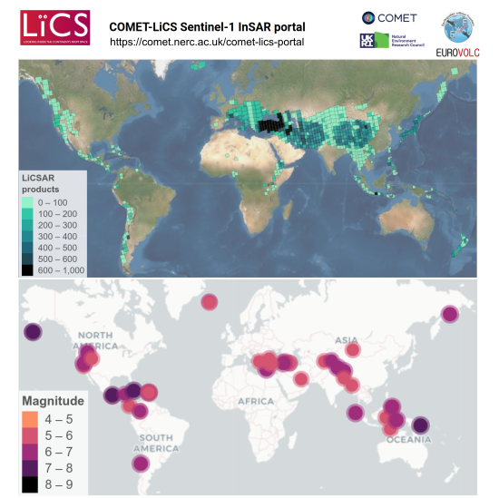Alternatively, the GEP’s Sentinel-1 Medium-Resolution InSAR Browse Service covers 38% of the world seismic mask, which represents over 15% of the Earth’s land masses, established by the Committee on Earth Observation Satellites (CEOS) based on [44]. Unlike the limited coverage by the GEP services, the Looking Into Continents from Space with Synthetic Aperture Radar (LiCSAR) system covers 1024 global volcanoes and aims to fully cover the CEOS world seismic mask area.

With slightly different aims, NASA Jet Propulsion Laboratory (JPL) has developed an Advanced Rapid Imaging and Analysis (ARIA) system, which automatically generates SAR-derived data products, primarily from the Sentinel-1 mission. It incorporates an automatic processing chain to generate co-seismic interferograms in response to major earthquakes and recently it has begun to provide standard InSAR displacement products, allowing users to circumvent the use of specialized radar processing software altogether and make InSAR products more accessible for science applications [45]. However, ARIA also does not currently plan to mass produce products over large regions for long time series analysis.

Here, we present activities carried out for the design, development, integration, and deployment of a fully automated state-of-the-art InSAR processing chain for Sentinel-1 data developed within the Looking Inside the Continents from Space (LiCS) project by the Centre for the Observation and Modelling of Earthquakes, Volcanoes and Tectonics (COMET). The LiCS project primarily aims at understanding how the continents deform at all spatial and temporal scales, with a focus on using observations of the earthquake deformation cycle to understand how seismic hazard is distributed in space and time. For this purpose, an automated InSAR processing system, LiCSAR, has been developed. LiCSAR is capable of processing Sentinel-1 data acquired globally, with the resulting products freely accessible and downloadable through an online portal, including both wrapped and unwrapped interferograms, coherence estimates, time series and other products. Innovative algorithmic, processing and storage solutions have been implemented to allow us to reduce the computing time and the required disk space.

This article is organised as follows. Section 2 presents the architecture and the main features of the LiCSAR processing system, providing basic information about facilities, data and metadata storage systems and processing chain strategies. Section 3 describes LiCSAR interferometric data products, their formats, structure and their update strategy. In Section 4, we will review how various tectonic, earthquake and volcanic applications benefit from the LiCSAR system, and illustrate this using recent results obtained in the Alpine–Himalayan belt. Conclusions and general plans for further developments of the system are given in the Section 5. As Appendix A, we include a list of abbreviations and brief explanation of external commands mentioned throughout the article.

2. LiCSAR System Architecture

The LiCSAR system consists of several interconnected modules. The LiCSAR processing chain, described in Section 2.1, uses various custom tools and algorithms over the core processing functionality that is based on advanced commercial software for processing SAR data, GAMMA [46]. The GAMMA programs mentioned within this article are described in Appendix A. LiCSAR processing is performed over systematic geographical spatial extents termed frames. A frame is defined as a collection of Sentinel-1 IWS burst units imaged during the satellite pass within a given orbital track. We have created custom LiCSAR burst unit identifiers. Metadata for each of these burst units are extracted from Sentinel-1 Single Look Complex (SLC) acquisitions and registered in the LiCSInfo metadata database that handles burst and frame definitions (see Section 2.2).

We extract and merge bursts covering a frame into SLC mosaics for each acquisition epoch. Afterwards, we coregister and resample these SLC mosaics to the geometry of a primary SLC acquisition, which is set during the initialisation of the frame. We then use the resampled SLC (RSLC) data to form interferometric products (wrapped and unwrapped interferograms, and coherence maps) by combining the new RSLC with, by default, four chronologically preceding ones, and georeference them to the World Geodetic System 1984 (WGS-84) coordinate system. The whole process is automated and optimised for effective batch processing in computer clusters, and identified as the LiCSAR FrameBatch toolbox, described in Section 2.3. LiCSAR FrameBatch is a standard tool used for updating frame datasets and is called by other specific tools, such as LiCSAR Earthquake InSAR Data Provider (EIDP), described in Section 2.4.

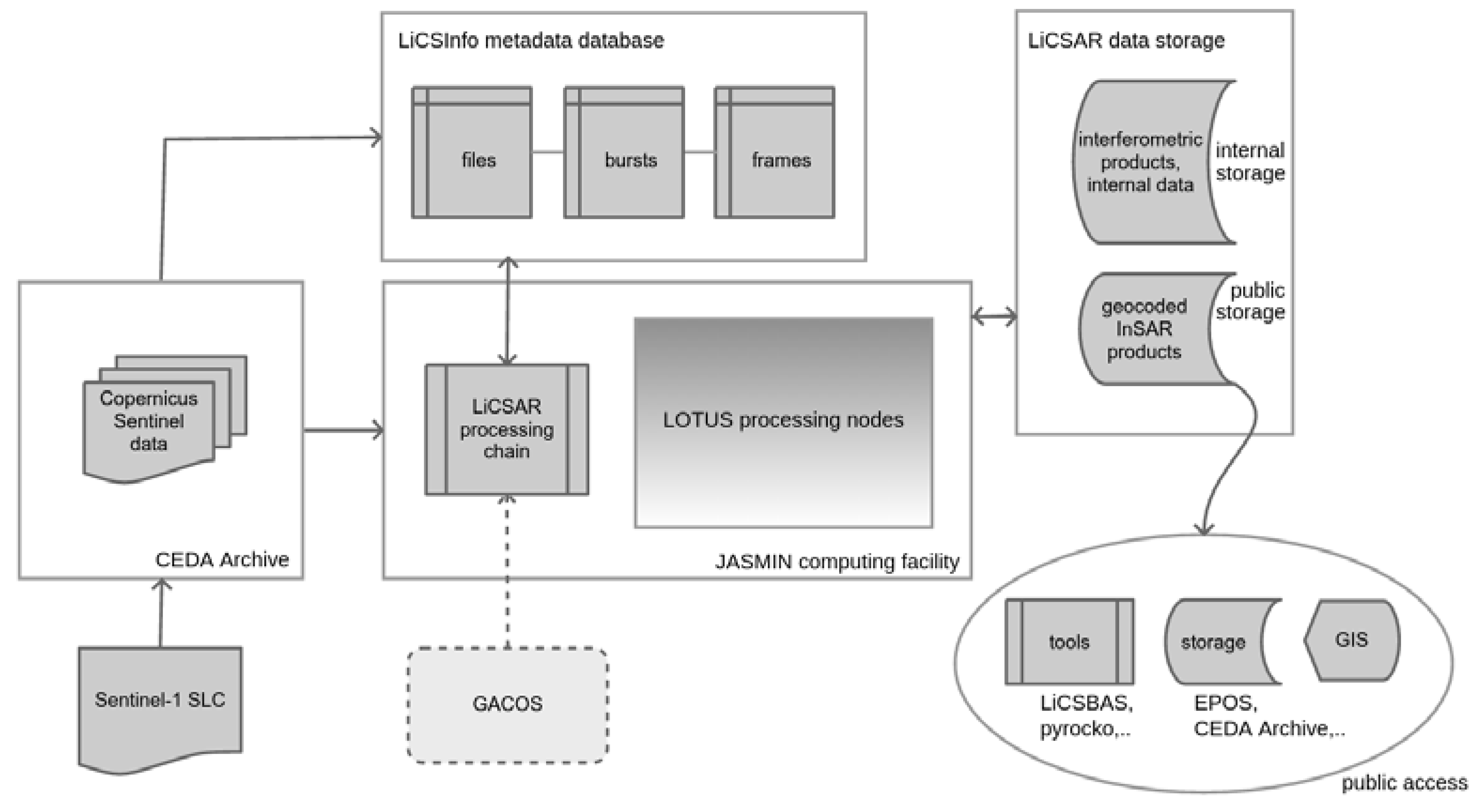
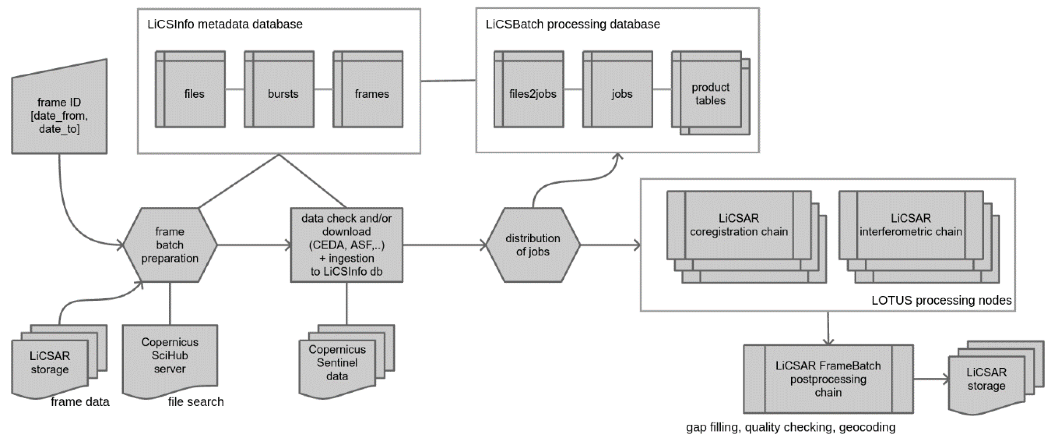
We show a general overview of the LiCSAR system architecture in a flowchart in Figure 1. The whole system is closely aligned to the technical infrastructure offered by the Centre for Environmental Data Analysis (CEDA), see Section 2.5. Here, both data storage (CEDA Archive, internal and public LiCSAR data storages) and computing facilities are synchronised with the LiCSInfo database (see Section 2.2) and LiCSAR processing chain to prepare InSAR outputs.

The flowchart in Figure 1 also shows a connection to the COMET Generic Atmospheric Correction Online Service (GACOS) system [47], allowing for optional routine corrections of tropospheric delay in interferograms using atmospheric weather models. The procedure to acquire GACOS data has not been fully automated yet, as the current API requests for generating GACOS data would prolong the LiCSAR product generation process. GACOS data per frame are currently being generated upon request and provided to the community. The impact of the optional GACOS corrections has been tested in Anatolia, where the correction reduced the phase standard deviation in interferograms by 20–30% [48].

2.1. LiCSAR Processing Chain

The aim of the LiCSAR processing chain is to generate interferometric products (see Section 4.1.1). The processing workflow to generate interferometric products by LiCSAR is outlined graphically in Figure 2. Prior to this workflow, each frame should be first defined and initialised within the LiCSInfo database. While frame definition means a logical linking of burst definitions within a frame unit, the initialisation of the frame means a status of having generated base frame data, including the primary epoch SLC and its multilooked intensity raster (MLI), height values based on a digital elevation model (DEM), and other frame-related derived products, such as the three components of the unit vector in the satellite line-of-sight (LOS) for each pixel, which define the sensitivity to motion in the East (E), North (N) and upward/vertical (U) directions [49]. We currently use a 1 arc-second void-filled version of the Shuttle Radar Topography Mission (SRTM) DEM as the basic DEM to derive the base frame data [50]. For cases of regions outside the SRTM DEM coverage, we have lately started to use the freely available WorldDEM product (https://geoservice.dlr.de/web/dataguide/tdm90) by Deutsches Zentrum für Luft (DLR) based on TanDEM-X satellite measurements provided in 3 arc-seconds resolution. In exceptional cases, some frames are prepared using other topographic models. For example, most of the frames from Sentinel-1 Stripmap mode (SM) use the 1 arc-second ALOS World3D DEM, https://www.eorc.jaxa.jp/ALOS/en/aw3d, by Japan Aerospace Exploration Agency (JAXA) based on Advanced Land Observing Satellite (ALOS) measurements; some older frames used 1 arc-second ASTER Global DEM product, https://asterweb.jpl.nasa.gov/gdem.asp, by NASA JPL and the Ministry of Economy, Trade and Industry of Japan (METI), based on data from the Advanced Spaceborne Thermal Emission and Reflection Radiometer (ASTER) satellite. The DEM-based frame data are key for geocoding of the products and estimation/removal of interferometric phase due to topography. Following subsections provide an overview on the four steps of our interferometric processing of Sentinel-1 data for each temporal epoch.

2.1.1. Preparation of Frame Epoch SLC

In the first step, we identify Sentinel-1 SLC data covering a given temporal epoch (a given date) and containing all or at least some bursts of the given frame definition. Frame burst data are extracted from related files available from some of the source data stores (see Section 2.5) and merged to form a frame epoch SLC. We perform several operations at this stage of processing. Firstly, we apply precise (21 days delay) or restituted orbit ephemerides data generated by the Sentinel-1 Quality Control Subsystem (https://qc.sentinel1.eo.esa.int) and downloaded daily from ASF DAAC. We perform a basic set of checks and corrections, such as padding of missing burst data with zeroes (in case of burst data unavailability for the given epoch), or correction of some known issues, e.g., an azimuth phase shift of −1.25 pixels in the first swath for older data (typically before April 2015) processed by Instrument Processing Facility (IPF) software version 2.36. Finally, we generate an MLI image using our default parameters, e.g., numbers of looks (4 for direction in azimuth and 20 in range), leading to a pixel spacing of 56 × 46 m (azimuth × range) in the LOS direction.

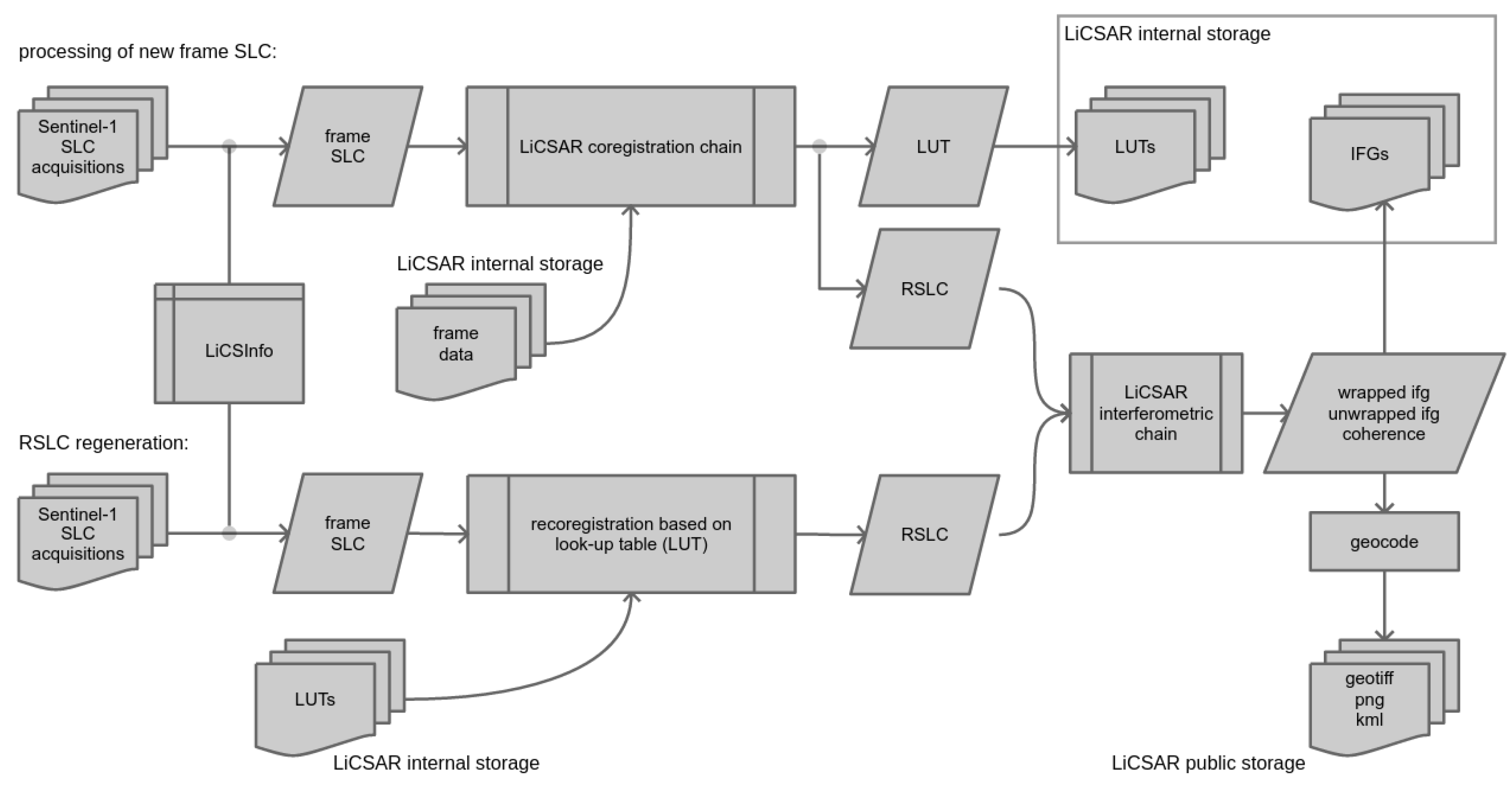
2.1.2. Resampling to RSLC

The resampling step is demanding on random-access memory (RAM) and has the longest processing runtime—over 1 h per epoch using a single processing core. The task of this step is to generate resampled RSLC files and additional supplementary files that can be used later to regenerate RSLC if needed for data reprocessing. The process of generating RSLC and the supplementary files from the epoch SLC is shown in Figure 3. The following textual description uses estimated processing time (EPT) measured for a typical frame consisting of 39 bursts (13 bursts per swath) and using a single processing core (as experienced at the facility described in Section 2.5). The resample procedure (including precise coregistration) follows the approach implemented within the GAMMA command S1_coreg_TOPS.

After the first step of generating an epoch SLC (and MLI), a frame DEM (also multilooked by factors of 4 × 20) is used to provide a DEM-assisted SLC coregistration (GAMMA command rdc_trans, EPT ~2 min). A preliminary coregistration lookup table (LUT) is generated. In order to increase the precision of SLC coregistration, an intensity cross correlation is performed towards the frame’s primary SLC image (GAMMA command offset_pwr_tracking, EPT ~5 min) and the estimated offsets are used to update the LUT.

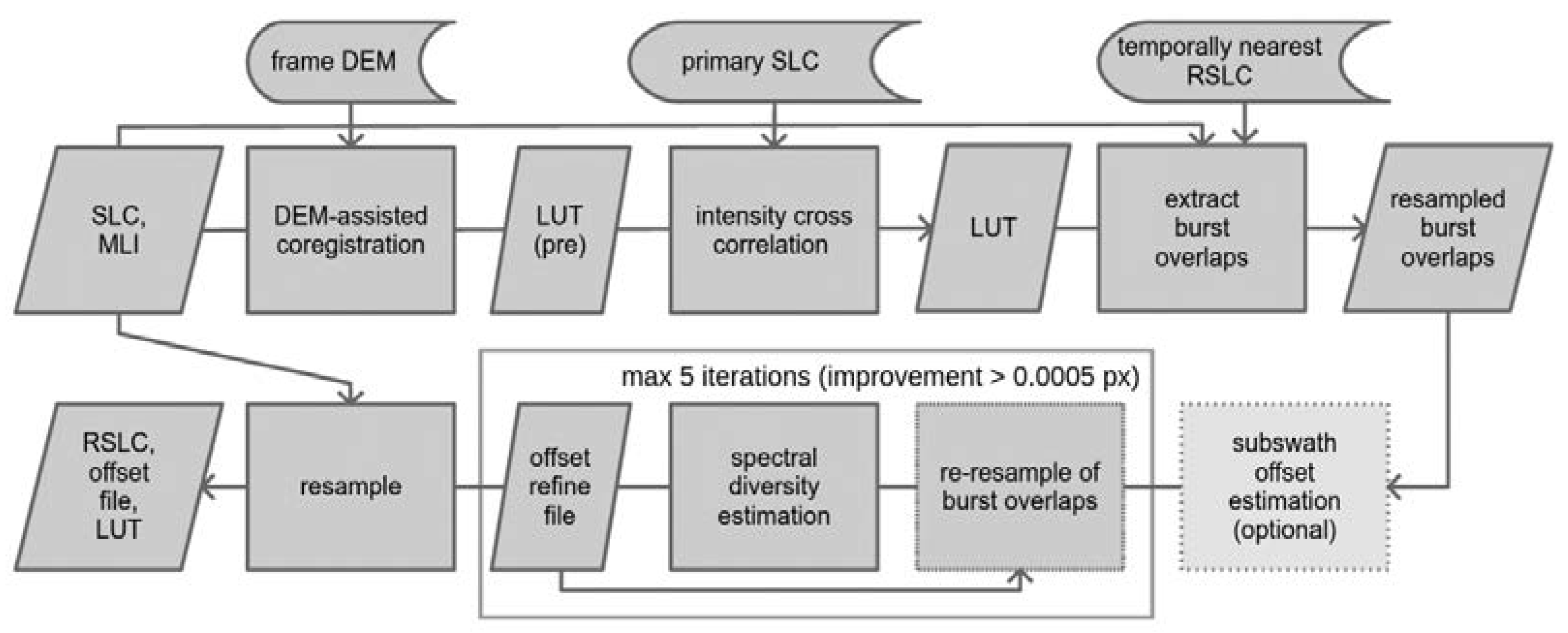
In order to achieve the high precision coregistration required for interferometric processing of a specific Terrain Observation with Progressive Scan (TOPS) mode of the Sentinel-1 IWS data [51], we use the spectral diversity (SD) technique [51] that estimates a mis-registration offset in azimuth direction, based on inversion of azimuth ramps in interferograms formed from overlaps between bursts of primary and secondary SLC images. To keep a reasonable coherence in the burst overlap interferograms and thus increase reliability of the SD estimate, an existing RSLC is used instead of the primary SLC if its epoch is closer to the epoch being coregistered—this temporally nearest RSLC is recognised as RSLC3. The primary SLC can also serve as RSLC3.

Prior to the SD estimation, a subswath offset estimation (GAMMA command S1_coreg_subswath_overlap, EPT 15 min) is applied to datasets being processed by an IPF differing from the original primary SLC; currently this step is applied only to data from the problematic IPF 2.36.

To estimate the mis-registration using SD, we determine burst overlap regions from the primary SLC metadata (GAMMA command S1_poly_overlap). Raster coordinates of the burst overlap regions are used to generate a masked LUT. The masked LUT is applied to resample only the burst overlap regions of the secondary SLC (EPT 20 min). The SD azimuth offset is estimated in the burst overlaps between the secondary SLC and RSLC3 by applying GAMMA command S1_coreg_overlap (to determine the fine coregistration offset within the burst overlaps) on the overlap region resampled towards the RSLC3. If the coregistration offset changes by more than 0.0005 pixels, the resample and coregistration of the burst overlaps is repeated up to 5 times (EPT 60+ min). This threshold should allow for further interferometric combinations of any RSLC data with maximal residual azimuth ramp of approx. 0.05 rad [52]. Finally, the azimuth pixel offset w.r.t. the LUT is estimated and both are used to resample the original secondary epoch SLC into the RSLC.

After the resampling process, the LiCSAR system stores the LUT and the estimated subpixel shift in azimuth direction (SD estimate) inside an offset refinement file for each RSLC. The LUT and offset refinement files can be used later if needed to quickly regenerate an RSLC from SLC data.

2.1.3. Formation of Differential Interferograms

After ensuring the RSLC mosaics exist for a selected interferometric combination, a simulated DEM-based interferogram is formed containing a prediction of the topographic phase. This topographic phase is removed during the formation of a standard 4 × 20 multilooked interferogram (GAMMA commands phase_sim_orb and SLC_diff_intf). By default, interferograms are formed between each epoch and the four preceding and/or following epochs (EPT 15 min/interferogram).

2.1.4. Unwrapping Interferograms

The interferogram unwrapping is performed using snaphu in version 2 [53]. Prior to the unwrapping process, the interferogram is spatially filtered using an adaptive power spectrum filter [54] (GAMMA command adf with the parameters FFT window size = 32 and alpha = 1.0). The default filter parameters were chosen based on experience towards monitoring large-scale deformations; however, they can be overridden by a local configuration file per frame. Points with interferometric coherence lower than 0.5 after filtering are removed prior to unwrapping. A map of statistical costs is generated based on a custom approach that searches for phase consistent pixels, avoiding false phase jumps within a threshold distance [55]. The unwrapping process is run on a single core with no tiling (EPT ~15 min/interferogram).

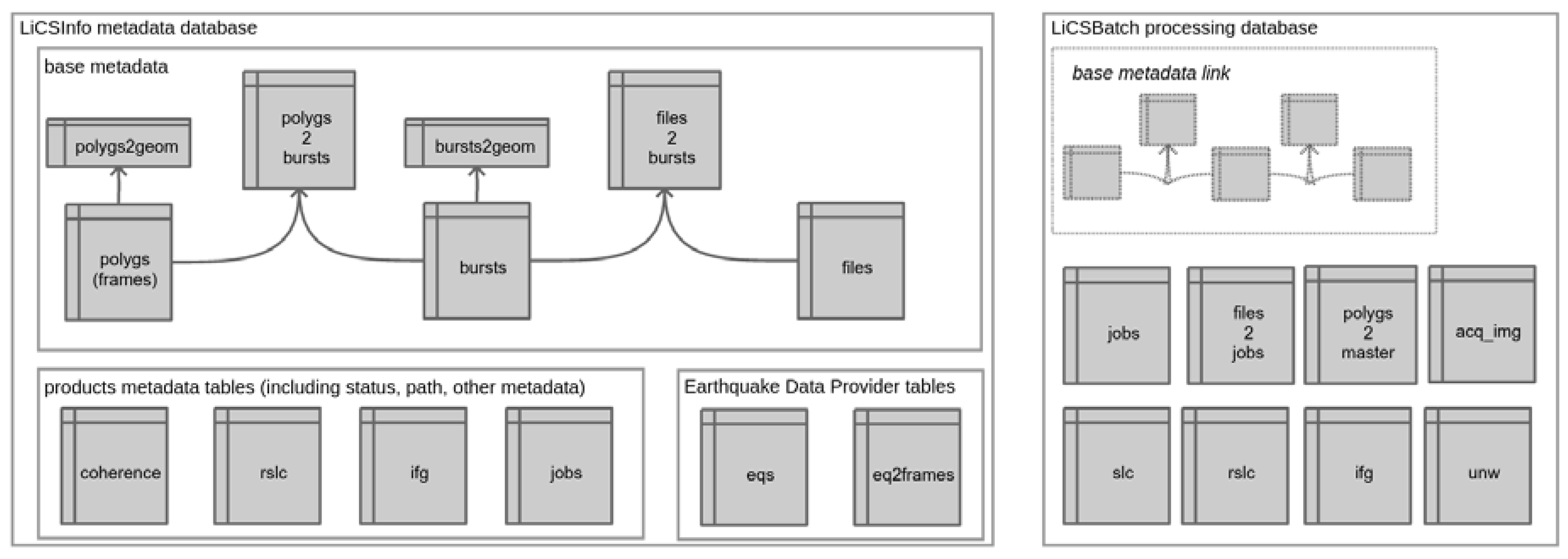
2.2. LiCSInfo Metadata Database

The LiCSInfo metadata database has been developed as the core for our autonomous Sentinel-1 processing system. It contains information on the original Sentinel-1 SLC data files, the LiCSAR frame definitions and the links between them through common burst units. It also stores basic information on processed interferometric products (e.g., file paths, perpendicular baseline) and other useful information (e.g., number of unwrapped pixels as a measure of the product quality). The database is also used to maintain frame update triggers if a frame is set as ‘active’. The base structure of the database is depicted in Figure 4.

Sentinel-1 IWS acquisitions in the form of SLC data are originally distributed as a set of focused burst units (or bursts) within three swaths. Burst metadata, including the geographic coordinates of each burst, can be directly read or inherited from Sentinel-1 annotation files provided within the distributed data. We generate custom unique LiCSAR burst identifiers based on the Zero Doppler azimuth time of the first line of the burst relative to the Ascending Node Crossing (ANX) time. The information is ingested to the table bursts. In the case of Sentinel-1 SM mode acquisitions, the whole areal coverage of the image is set as a burst.

Frame definitions are stored in the table polygs. The table includes the generated frame identifier (the naming convention is explained in Section 3) and geographic coordinates of frame corners, among other metadata. The geographic coordinates are generated either from the set of bursts comprising the frame in the case of IWS products or they are set to cover a particular area of interest in the case of SM frames. The bursts are linked to the related frames through a lookup table polygs2bursts. Geodatabase functions are enabled through tables bursts2geom and polygs2geom, for both bursts and frames.

Having the basic information about ingested SLC files stored in the table files and linked to bursts contained within the files through the lookup table files2bursts, it is possible to perform SQL queries such as identifying files related to requested epochs within a selected frame. These structures are also linked to a concurrent LiCSInfo batch processing database (LiCSBatch database) that is used within the LiCSAR FrameBatch processing chain (see Section 2.3). Here, temporary fields linking job-relevant files and bursts are stored in interconnected LiCSBatch tables, as shown in the right panel of Figure 4. Final product information can be stored in product metadata tables (coherence, rslc, ifg).

Finally, the Earthquake Data Provider tables include basic information on earthquakes and related frames that are ingested to processing by the LiCSAR Earthquake InSAR Data Provider system (see Section 2.4). These tables keep track of processing stages for generating pre-seismic, co-seismic and post-seismic interferograms.

2.3. LiCSAR FrameBatch Processing

The LiCSAR FrameBatch package is a set of data structures and algorithms designed to automate frame processing using LiCSAR. It is optimised to run on a computing cluster facility. Our frame processing strategy consists of four parts described below and depicted in Figure 5. The only required user parameters for starting batch processing for a frame are the frame identifier, a toggle for “auto-download” functionality, and, optionally, a start/end date.

2.3.1. Data Preparation

At the initial stage, base frame data (pre-processed primary epoch SLC, MLI, DEM-derived frame products etc.) are copied from LiCSAR internal storage to a temporary BatchCache folder. Any products stored in LiCSAR internal storage covering the frame during the requested time period are either linked (interferometric products) or decompressed (coregistration LUTs or RSLCs, compressed using 7zip). We then use a data-filling script to search for the existence of relevant Sentinel-1 SLC data by querying Copernicus SciHub (https://scihub.copernicus.eu), comparing the SciHub list to information on the data already ingested to the LiCSInfo metadata database, checking and optionally auto-downloading the relevant SLC data, and then refilling the LiCSInfo database. Optionally, the routine can be set to request the data available at CEDA storage from their Near Line Archive system (NLA, see Section 2.5) automatically, though the user is expected to perform such a request prior to the FrameBatch processing (non-autonomous NLA requests are preferred as the complex mechanism of the NLA may induce significant delays in the whole frame processing).

2.3.2. FrameBatch Processing Chain

After the data preparation step, we generate frame batch processing job definitions. First, epochs covering the requested time period are identified based on LiCSInfo database entries (selecting ingested files that contain bursts related to the frame definition). The epochs are then distributed into processing job definitions for LiCSAR processing steps: SLC generation, coregistration into RSLC, generating interferograms and unwrapping. A maximum of 5 job definitions per step are generated for cases where processing covers the last 3 months (i.e., covering up to 15 epochs, thus distributed into processing of up to 3 epochs per job); a maximum of 20 jobs per step are generated in case of larger requested time scales. A special LiCSBatch database interconnected to LiCSInfo is used—it contains tables allowing us to identify epochs related to each job definition and to keep track of the progress of jobs. The interferogram generation and unwrapping steps are set to create the standard set of combinations of every epoch with the four preceding epochs.

After the LiCSBatch cache is ready, the processing jobs are started in parallel. Follow-up steps only begin once the preceding steps are finished for given epochs. The processing jobs are optimised to run for less than 24 h each. Only one processing core is requested per job. Though this approach does not take advantage of the increased effectiveness of parallel processing algorithms (e.g., GAMMA scripts or snaphu), it allows requesting a larger number of parallel jobs in the computing cluster environment.

2.3.3. FrameBatch Post-Processing

The final stage consists of the following operations: a gap-filling script checks for non-existing wrapped and unwrapped interferograms and runs parallel jobs to generate InSAR products in standard combinations (4 preceding epochs, based on a set of successfully generated RSLCs) and a geocoding script georeferences InSAR products in the georeferenced Tagged Image File Format (GeoTIFF) in the WGS-84 coordinate system and their previews in Portable Network Graphics (PNG) or Keyhole Markup language Zipped (KMZ) formats. An optional routine stores relevant files in the internal LiCSAR storage and the public LiCSAR folder and cleans the temporary processing directory and LiCSBatch cache.

We have developed a specific interferogram quality check routine that is applied before the automatic data store. In this routine, we identify artifacts such as SD estimation errors and coregistration issues using a line detection algorithm. We also employ a normalised mean coherence and fraction of number of unwrapped pixels w.r.t. existing set of interferograms, in order to identify corrupted interferograms by a predefined threshold value.

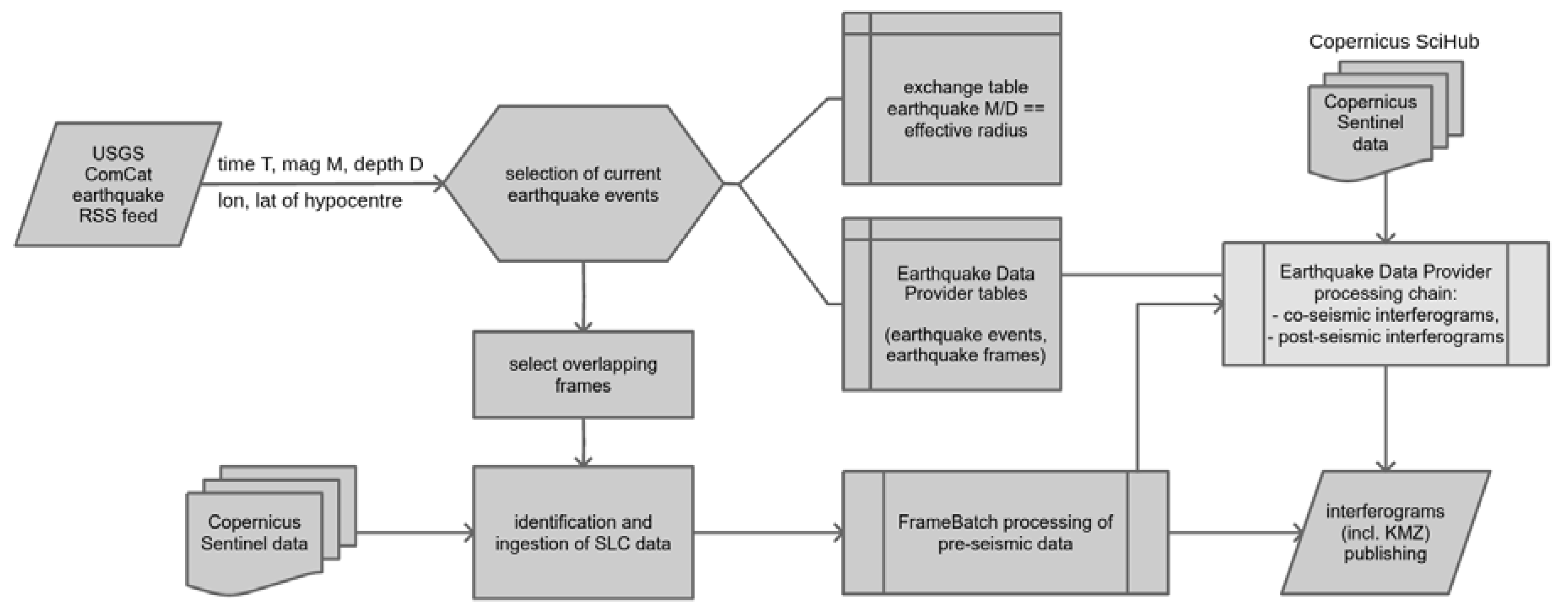
2.4. LiCSAR Earthquake InSAR Data Provider

The rapid availability of Sentinel-1 data following acquisition (a few hours), together with the short revisit period, for many areas, of 6 days, provides a unique opportunity to develop an automatic earthquake response system using the LiCSAR infrastructure. The main objective of this response system is to form co-seismic interferometric pairs in a rapid manner, as well as pre- and post-seismic interferograms, and to make these data widely and freely available to the community. We anticipate that these products have applications for the scientific understanding of events as well as for operational crisis management and disaster mitigation.

The automatic Earthquake InSAR Data Provider (EIDP) within the LiCSAR system works as follows (Figure 6): a list of current earthquake events with a minimum magnitude of M_w 5.5 is requested through a libcomcat python library [56] providing access to the USGS Comprehensive Earthquake Catalog (ComCat). We then generate a look-up table to estimate the potential radius of the region in which surface deformation caused by the earthquake may have occurred, given the estimated seismological magnitude and 3D location of its hypocentre, accounting for uncertainties in the seismological estimates (see

Table 1. Earthquake response threshold criteria for the Earthquake InSAR Data Provider (EIDP), based upon empirical scaling of fault dimensions with magnitude and anticipated wavelength of measurable surface displacement of a buried elastic source. The postseismic interval indicates the length of time the near-real time processing by EIDP is undertaken, prior to return to their regular processing.

Magnitude [Mw]	Max. Depth of Hypocentre [km]	Surface Effect Radius from Epicentre [km]	Postseismic InSAR [Days after Earthquake Event]
5.5–5.9	10–16	20–30	18–36
6.0–6.9	18–63	36–167	30–84
7.0–7.9	73–250	199–938	54–132
8.0–8.5+	250	1115–2500	108–156

). This surface radius is used to select all overlapping frames, using the frame definitions from the LiCSInfo database. In the case that a selected frame has not been previously initialised, an automatic initialisation is attempted. We then update the EIDP-related tables in the LiCSInfo database and process at least the last month of data associated with the selected frames using standard LiCSAR parameters and the LiCSAR FrameBatch approach.

We have developed routines for the early identification and fast download of the first post-earthquake Sentinel-1 data and we have created an automatic download routine that uses the Copernicus SciHub service as an alternative data source in order to ensure the availability of the latest data for processing—Sentinel-1 SLC data typically arrive at Copernicus SciHub within a few hours post acquisition, which is earlier than they appear in other accessible data mirrors.

As we use image cross-correlation algorithms within the LiCSAR coregistration step (see Figure 3), the RSLCs can be generated successfully even without the use of precise orbital ephemerides. Instead, restituted ephemerides (existing already at the time of appearance of the source Sentinel-1 data) are downloaded and applied automatically. We also export co-seismic interferograms as Google Earth KMZ files, in addition to standard InSAR outputs. After a basic quality check, we link the co-seismic interferogram products to our web-based LiCSAR EIDP map and prepare structures for their automatic ingestion to other community systems (see Section 3). We also aim towards integration of GACOS atmospheric phase screen correction estimates to the final interferograms, noting that GACOS data should be available with a 24 h delay.

From the perspective of the system architecture, we have been using a sequential procedure that generates coseismic interferograms within 24 h after the post-event SAR data acquisition. This has been lately substituted by a solution that allows us to reach co-seismic interferograms within 1–3 h after the appearance of post-event Sentinel-1 SLC data on the Copernicus SciHub web service. The major difference is a specific integration of a dedicated computing node at a distant computing facility for resampling the post-event data with the use of parallel processing and rapid generation of interferometric products. Here, the EIDP system controls the processing stages in 30 min ‘ticks’. One tick is a series of operations to ingest new events to the EIDP database tables, identify earliest and expected post-event acquisition times, send frame preprocessing job requests, check and download available post-event data, send processing jobs for generation of co-seismic and post-seismic data, and finally update information about the processing status to EIDP tables.

The frames remain in their active status for a pre-defined period to allow for rapid production of post-seismic interferograms (a post-seismic InSAR response). We scale this time period depending on the magnitude of the event and the number of expected Sentinel-1 images in that location, see Table 1. In case of very large events, the post-seismic interferograms are further generated by LiCSAR continuous rolling updates that are being performed on straining regions (see Section 3.1). We also plan to extend the system to volcanic activity rapid response.

2.5. Processing and Storage Facility

The LiCSAR processing and storage system runs on CEDA’s data analysis infrastructure JASMIN [57]. JASMIN is a computing facility designed for environmental data analysis supercomputing. The processing is carried out mainly using a Load Sharing Facility (LSF) for distributed computer clusters named LOTUS. Since September 2018, JASMIN offers over 40 PB of storage and over 10,000 computing cores distributed between the LOTUS computing cluster and a community cloud [57,58]. LOTUS is managed through a queuing system, which allows splitting of large processing jobs to run on a requested number of computing cores reserved from LOTUS computing nodes. As we use a dedicated processing queue with a limit of a maximum number of 128 reserved computing cores, we do not use parallel processing algorithms but rather send larger numbers of processing jobs by reserving one computing core per job.

A community cloud service at CEDA offers managed cloud instances, which we use to run a MySQL/MariaDB database system dedicated to the LiCSInfo database.

Apart from a 350 TB disk area for permanent internal, publicly shared and temporary LiCSAR output files, the JASMIN infrastructure offers direct access to a CEDA Sentinel Mirror Archive (SMA), a service mirroring data from the Copernicus Sentinel programme [59]. Currently, SMA contains more than 2 PB of data or ~1.6 million individual Copernicus Sentinel data products, over 60% of which is Sentinel-1 SLC data [57]. To cater to the increasing amount of Sentinel data, CEDA has developed the Near Line Archive (NLA) system. The NLA is used to archive older data onto a modern tape storage system. This brings about the limitation of having only the newest data (acquisitions younger than 3 months) available on disk via instant access. Archived data can still be requested—it should take no longer than 24 h to retrieve data from the NLA into its original location in the SMA directory structure. The restored data can be accessed for a limited period of time (typically 3 weeks). Therefore, the Sentinel-1 data does not have to be downloaded before processing, greatly reducing the time necessary to obtain results.

In cases where the requested Sentinel-1 data are not available at SMA, we use one of the optimised high speed transfer servers at the CEDA JASMIN facility to download the required data from either NASA’s ASF DAAC or the Copernicus SciHub server. The necessary SLC datasets are normally available on Copernicus SciHub within a few hours of the satellite acquisition.

Finally, we have established a dedicated computing node at the University of Leeds supercomputer (ARC4, http://arc.leeds.ac.uk) that serves as a stable extension of the LiCSAR system, primarily running at CEDA facility. We use the node for running the LiCSAR EIDP service.

3. LiCSAR Products: Current State and Future Trend

The basic InSAR products generated by LiCSAR are original and spatially-filtered wrapped, as well as unwrapped, interferograms and original coherence maps, MLI images for each epoch, and complementary specialised frame images, including incidence angle map files needed for motion vector extraction [49], height values from the DEM used in processing, preprocessed GACOS products, and metadata information (e.g., perpendicular baseline list, date and acquisition time of the primary epoch image). The provided products are georeferenced to the WGS-84 geographic coordinate system. After the processing, results are shared in the form of GeoTIFF files and preview bitmap rasters (in PNG format, downsampled to 30% of the original GeoTIFF’s dimensions). Some products of special interest (e.g., co-seismic interferograms) are converted into Google Earth KMZ files. In Section 3.1, we elaborate on the contents and coverage of the products.

The LiCSAR products are publicly available through the COMET LiCS products web portal (currently at https://comet.nerc.ac.uk/COMET-LiCS-portal) in the structure described in Section 3.2. Selected InSAR products are or will be available within the European Plate Observing System (EPOS) (http://www.ics-c.epos-eu.org), and the CEDA Archive (https://catalogue.ceda.ac.uk), as well as other platforms (e.g., Google Earth Engine).

3.1. Contents, Coverage and Update Strategy of LiCSAR Frame Products

LiCSAR systematically uses Sentinel-1 IWS SLC data to generate large-scale multilooked interferograms, georeferenced to the ground resolution of a pixel size of 10⁻³ × 10⁻³ degrees in the WGS-84 geographic coordinate system (corresponding to ~100 × 100 m at the equator). Sentinel-1 datasets are processed, organised and catalogued in frame units. Default frames consist of 39 bursts (13 bursts within each of three observation swaths)—such a standard frame covers an area of around 220 × 250 km. Our standard frame definitions include overlap of one burst per swath with each neighbouring frame along the orbital track. This enables us to seamlessly merge interferometric outputs from the frames.

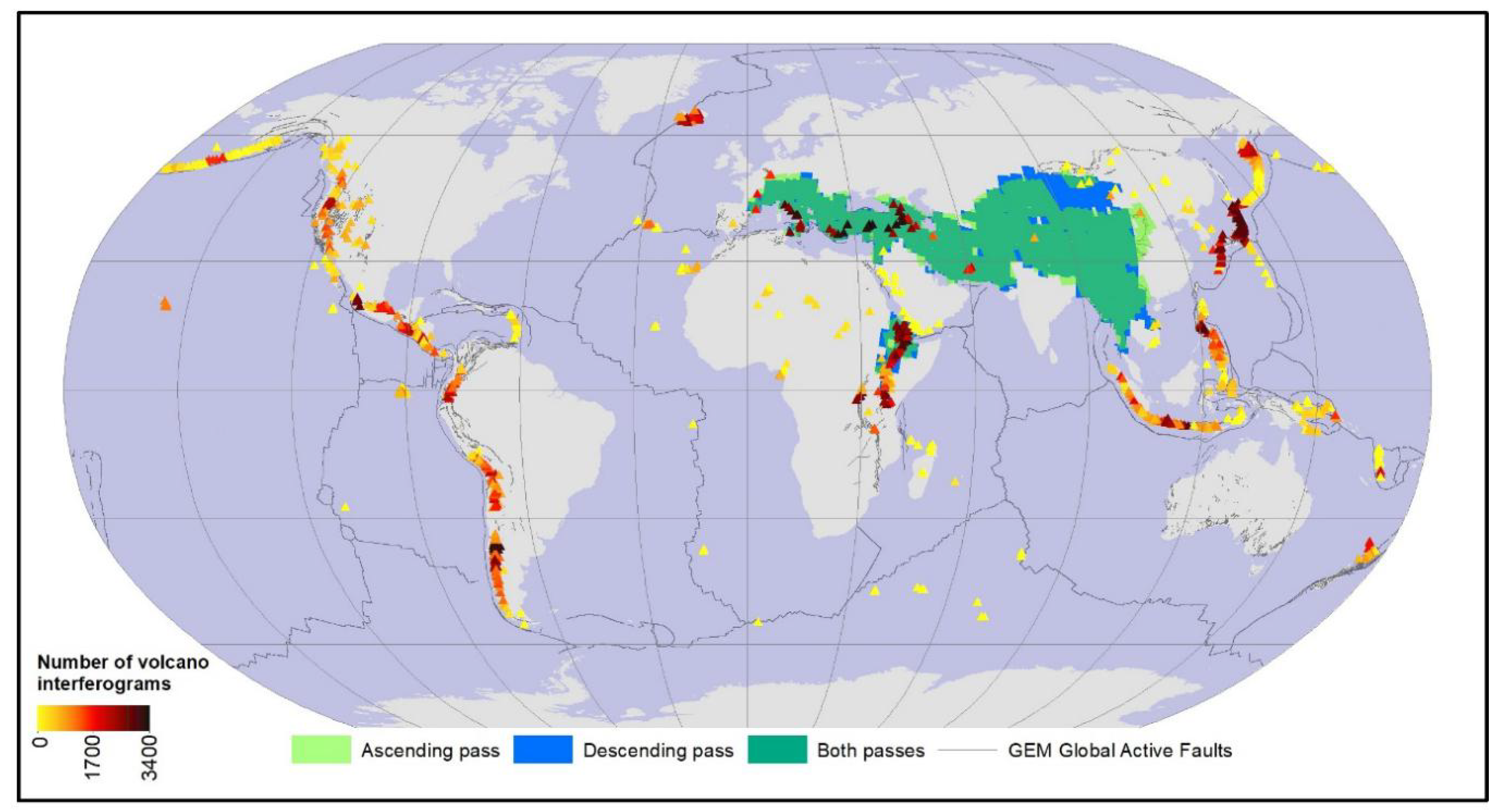
We have defined frames globally, but only carry out systematic LiCSAR InSAR analysis on a selection of frames within our current priority areas. The tectonic priorities are the Alpine–Himalayan Belt (572 frames) and East African Rift System (Figure 7). These frames are currently in the process of being systematic backfilled to a monthly ‘rolling’ status, in which data will be no more than 1 month out of date. This default status allows us to use the precise orbit ephemerides, which are available 21 days after each acquisition. Frames of a special interest can be switched to a weekly ‘rolling’ status with interferograms generated using the latest available data (using restituted orbit ephemerides).

The LiCSAR system is also producing Sentinel-1 frame interferograms globally over 80% of the 1331 on-land volcanoes considered active during the Holocene [60]. Frames covering areas with volcanic activity are being updated three times per week and the list of these frames is updated based on new and ongoing volcanic activities reported by the Smithsonian Institution [60]. Figure 7 shows the global distribution of the active volcanoes and the number of interferograms for each of them. We develop routines to augment these frames into a ‘live’ status, i.e., to have interferograms generated as soon as a new acquisition appears at some of our source data stores.

Interferograms related to recent seismic events are generated by the LiCSAR EIDP processes. Figure 7 includes locations of earthquakes where LiCSAR generated co-seismic frame interferograms. The frequent updates of earthquake-related frames (by EIDP) ensure their temporary ‘live’ status until a specified time after the earthquake (in order to also generate several post-seismic interferograms).

Due to ESA’s acquisition strategy for Sentinel-1, some of the data collected over certain small islands is acquired in SM mode. SM acquisitions are obtained in one of six possible beams. These beams cover a range of incidence angles of approx. 22–44° and acquire data in a finer pixel spacing of 1.5–3.1 × 3.6–4.2 (slant range × azimuth) [62]. LiCSAR automated processing produces interferograms for these regions, multi-looked to ~30x30 m resolution, and the same output files and metadata as are generated for IWS acquisition mode products. We have added an automatic processing functionality for SM acquisitions to incorporate the following volcanic islands to the LiCSAR product database: La Réunion (French territory, Indian Ocean), Fogo (Cabo Verde), Tristan da Cunha (British Overseas Territory, south Atlantic Ocean) and Marion Island (South Africa, sub-antarctic Indian Ocean). To keep SM frames consistent with the LiCSAR system architecture originally designed for IWS data only, we use the geographic area of the SM image as a “burst” in the LiCSInfo database and a subset definition (geographic coordinates of corners covering area of observed island) as a “frame”.

One of the major limiting factors of the use of the InSAR in most of tectonic and volcanic applications is the spatiotemporal variability of tropospheric properties. This is of importance, especially in cases where deformation and topography are correlated [63]. To address this limitation, we have developed tools for including products for an atmospheric correction, based on the COMET GACOS system developed at the University of Newcastle [47]. GACOS uses an iterative tropospheric decomposition interpolation model that decouples the elevation and turbulent tropospheric delay components estimated from high-resolution European Centre for Medium-Range Weather Forecasts (ECMWF) weather model data and available Global Navigation Satellite System (GNSS) data. GACOS corrections are computed for each LiCSAR frame with the same image sizes to facilitate direct use.

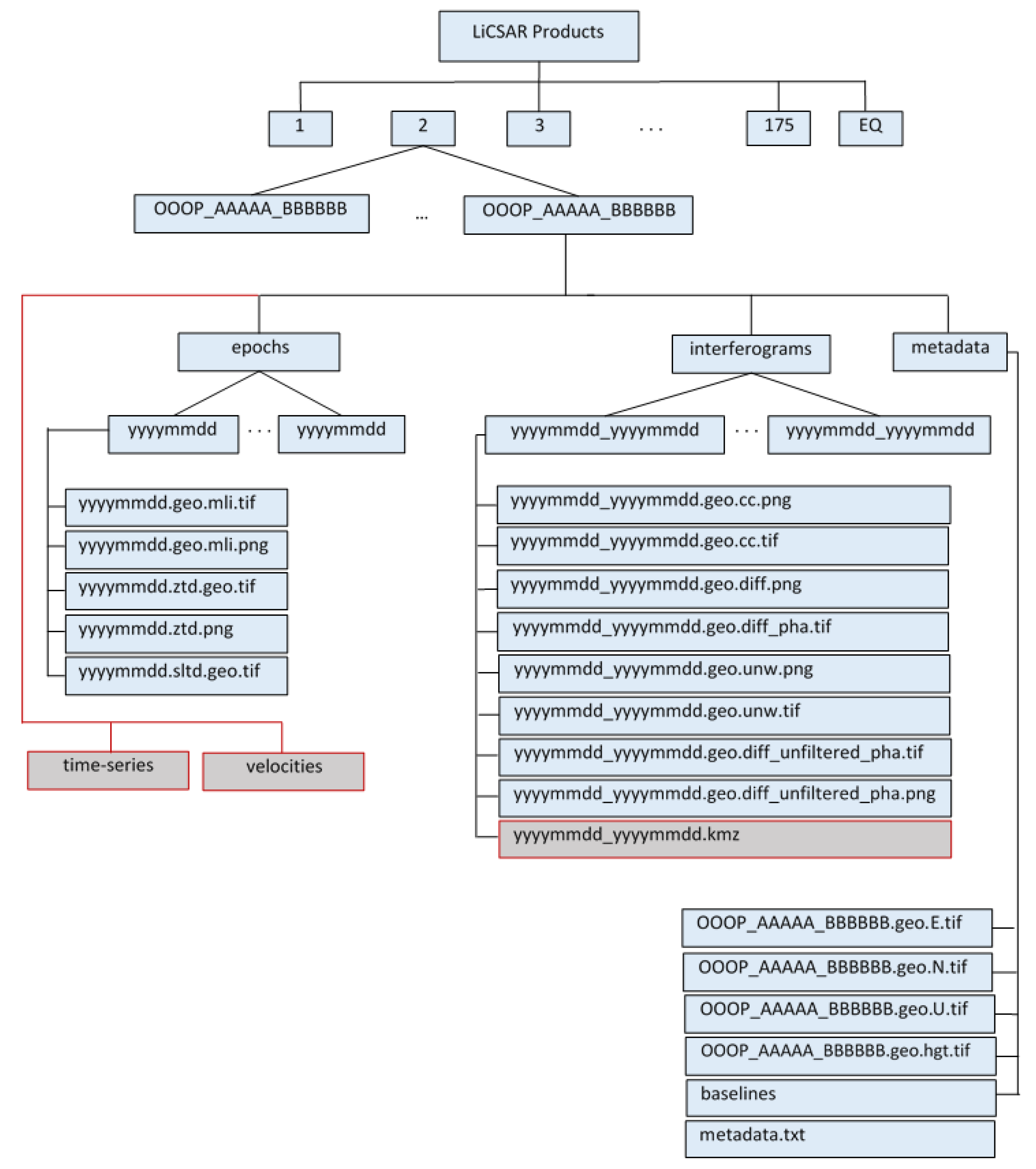
3.2. LiCSAR Products File Structure

Figure 8 shows the LiCSAR system file structure hierarchy and naming convention. The blue parts represent the current state and the gray areas show the capabilities that will be available in the future. Starting from the top level, the LiCSAR products are categorised into 175 folders that correspond to the 175 orbital tracks per orbital cycle (relative orbits) of the Sentinel-1 satellites. Currently, a special folder EQ contains geocoded outputs of the LiCSAR EIDP system categorised according to the USGS ComCat code for each earthquake (an updated dissemination platform is an ongoing process).

The naming convention of frame identifiers (used also as folder names for frame-related data) has a structure: OOOP_AAAAA_BBBBBB, where OOO denotes the number of the relative orbit, P identifies the orbital pass—either descending (D) or ascending (A), AAAAA is a colatitude identifier, i.e., a complementary angle of the latitude of the frame centre (multiplied by 100), and BBBBBB identifies the number of included bursts (three pairs of digits corresponding to number of bursts in each of three Sentinel-1 IWS swaths).

Inside the frame directory, the generated InSAR products are located in the interferograms subfolder. The name of each interferometric pair shows the date of acquisition epochs used for that pair. The basic interferometric products reside in each interferometric pair folder as:

yyyymmdd_yyyymmdd.geo.cc.tif: coherence image (GeoTIFF) of the interferometric pair. The values vary between 1 and 255, where 1 refers to the lowest coherence values and 255 indicates the highest values of coherence. It is in uint8 format with 0 as the ‘no data’ value;

yyyymmdd_yyyymmdd.geo.cc.png: a gray-scale raster preview of the coherence image (white = maximal coherence). The preview is resized to 30% of the original GeoTIFF;

yyyymmdd_yyyymmdd.geo.diff_pha.tif: wrapped-phase spatially filtered differential interferogram image (GeoTIFF). The values vary within the range of -π to π radians. The phase values pertain to the the satellite LOS, thus the signal can be interpreted as motion away from the satellite if the observed phase difference is positive. The phase values are saved in the file in a float32 precision with 0 as ‘no data’ value;

yyyymmdd_yyyymmdd.geo.diff_unfiltered_pha.tif: wrapped-phase interferogram image (GeoTiFF). The only difference between this and the previous image is that the phases are not spatially filtered;

yyyymmdd_yyyymmdd.geo.diff.png: a raster preview of the wrapped-phase interferogram (a colour fringe in the direction blue–green–yellow–orange–purple–blue would mean a change of 2π radians towards the satellite). The preview is resized to 30% of the original GeoTIFF;

yyyymmdd_yyyymmdd.geo.unw.tif: unwrapped phase image in radians (GeoTIFF). Keeping the same rule as the wrapped phase images, the values are in the satellite LOS direction, i.e., positive values mean a range increase (i.e., motion away from from the satellite), while negative values mean a range decrease (i.e., motion towards the satellite) perhaps caused by uplift. The format of the file is float32 with zero values as ‘no data’ often related to pixels which are masked due to low coherence;

yyyymmdd_yyyymmdd.geo.unw.png: a raster preview of the unwrapped interferogram, representing interferometric phase values after rewrapping to a scale of 6π per colour cycle (using the same convention for LOS direction as for the wrapped-phase interferogram preview). The image is resized to 30% of the original GeoTIFF;

yyyymmdd_yyyymmdd.kmz: an optional Google Earth KMZ output is typically generated from full resolution (0.001°) raster previews of the generated interferogram products.

In addition to the interferograms, georeferenced MLI images for each processed epoch are stored in the epochs folder in directories corresponding to the acquisition date in the format yyyymmdd. The intensity images are produced by space–domain averaging of the SLC images with 4 and 20 as the number of azimuth and range looks, respectively. MLI images are generated without a radiometric calibration and only for a co-polarised channel.

Additional files are stored in the metadata folder:

OOOP_AAAAA_BBBBBB.geo.{E,N,U}.tif: these GeoTIFF files contain the E, N and U components of the LOS unit vector for each pixel. They are calculated from the SAR look-vector elevation and orientation angle of each pixel, based on the SAR imaging and DEM geometries with the local topography taken into account. The unit vector information can be used, for example, to project E-N-U modeling results or 3-dimensional geodetic observations like GNSS data onto the LOS vector in order to be able to compare them to the LiCSAR results [43]:

OOOP_AAAAA_BBBBBB.geo.hgt.tif: this image (GeoTIFF) contains the height values extracted from the DEM used in processing;

baselines: a text file containing the temporal and spatial baselines of each acquisition with respect to the master image;

metadata.txt: a text file containing various other information related to the frame (e.g., primary epoch and acquisition time for its center location, etc.)

In the near future, the time-series and velocity folders will contain outputs stemming from multitemporal InSAR processoring based on the LiCSBAS tool [64]. The main objective of this module (currently still under development) is to generate average displacement velocity maps and time series of displacements for all processed LiCSAR frames. The velocity and time series products will be provided initially in 1 km resolution, with a higher resolution (initially 100 m) over volcanic areas.

GACOS tropospheric delay maps are provided per epoch (in the epochs folder) in GeoTIFF format in the same resolution as the other LiCSAR products and in both vertical and LOS directions. The LOS tropospheric delay is stored as a yyyymmdd.sltd.geo.tif file. It should allow the user to readily apply the correction to the LiCSAR phase products, for example using the LiCSBAS software [64]. Additionally, we archive the original GACOS tropospheric delay map as yyyymmdd.ztd.geo.tif and yyyymmdd.ztd.png files. Currently, only a few frames have GACOS products generated during the testing phase.

4. LiCSAR Applications for Measuring Tectonic and Volcanic Deformations

Since the initial development of the LiCSAR system, numerous research projects have been carried out to study deformation of the Earth’s crust using LiCSAR products. Typical deformation sources include magma chambers, dike intrusions, and faults that slip during different phases of the earthquake cycle. In this section, we highlight some case studies where LiCSAR has contributed to the monitoring of tectonic activity and volcanic events.

4.1. LiCSAR for Tectonic Applications

Provision of Sentinel-1 InSAR products produced by the LiCSAR processor with a wide spatial coverage increases the potential for large-scale InSAR studies of tectonic processes. Over the past few years, the LiCSAR system has proved to be a powerful tool in various tectonic applications, leading to improved understanding of crustal deformation processes.

The LiCSAR system is currently producing Sentinel-1 interferograms for all the frames covering seisimcally active portions of the Alpine–Himalayan belt (9000 × 2000 km), where many of the planet’s most deadly earthquakes occur. The LiCSAR EIDP system is actively generating interferometric products for almost every major shallow earthquake affecting continental regions on Earth.

4.1.1. Coseismic Interferometric Products

As an example, Figure 9 shows three coseismic interferograms from continental earthquakes in different tectonic settings generated in both ascending (left) and descending (right) orbits. They correspond to the 4 July 2019, M_w 7.1 right-lateral strike-slip earthquake in Ridgecrest, California (Figure 9a), the 12 November 2017, M_w 7.3 dip-slip earthquake at the Iran–Iraq border (Figure 9b), and 16 September 2015, M_w 8.3 dip-slip earthquake in Illapel, Chile (Figure 9c). Each colour cycle can be interpreted as representing 2.8 cm of relative ground displacement in the LOS direction (i.e., towards or away from the satellite). Because the LiCSAR metadata folder includes grids of the unit vector in the satellite LOS at each pixel, the data can easily be used for earthquake source modelling, for example using tools such as Pyrocko [65], which automatically can ingest LiCSAR products.

As an example of other generated InSAR products, Figure 10a,b show the unwrapped phase and coherence images corresponding to the Ridgecrest interferogram in Figure 9b, respectively. It should be noted that the phases in Figure 10a are rewrapped to 6π and therefore the colour cycle here is equal to a 6π phase variation (8.3 cm if it is caused by movement in the LOS). The white areas in the unwrapped image show the areas that were masked based on a coherence threshold to avoid unwrapping errors. These low coherence regions (visible as dark spots in Figure 10b) can be due to large changes in the ground surface due to surface rupture, ground shaking and high displacement gradients. Figure 10c is the intensity image of the same frame corresponding to the post-seismic Sentinel-1 image, acquired on 21 August 2019.

4.1.2. Value-Added LiCSAR-Based Products for Tectonic Studies

An InSAR displacement time series serves as an example of products that can be generated using LiCSAR products. Interferometric products of LiCSAR over Turkey have been used to study the North Anatolian Fault (NAF), a major right-lateral, strike-slip fault accommodating the relative motion between the Anatolian and Eurasian tectonic plates at a rate of ~25 mm/yr [66]. We have processed LiCSAR frames for Anatolia starting with the first Sentinel-1A acquisitions in October 2014 until October 2019 to obtain the average satellite LOS velocities using LiCSBAS [64]. An example of a LOS velocity map for a selected frame, overlain by the main faults, clearly shows the right-lateral interseismic motion across the NAF (Figure 11a). Figure 11b shows the time-series of cumulative displacement for a sample pixel north of the NAF w.r.t. a reference pixel located south of the fault. The best-fit LOS velocity of −15.2 mm/year for this pixel is representative of the westward movement of the Anatolian microplate. We also see a clear seasonality to the relative LOS motion.

The global coverage of LiCSAR makes it possible to derive high-resolution, precise and global estimates of tectonic strain rate based on velocities from the LiCSBAS time series inversion [64]. The LOS velocities for the frame shown in Figure 11a have been used to derive strain rates for Anatolia after mosaicking with neighbouring frames using available GNSS data compilations in order to create seamless LOS velocity maps following the method outlined in [48]. Weiss et al. [48] also provide an estimate of LOS velocity uncertainties for the mosaicked frames, which are on the order of ~2–3 mm/yr and largely depend on the uncertainties of the GNSS data [64].

4.2. LiCSAR for Volcanic Applications

The total number of interferograms calculated for volcanoes is greater than 364,400 (as of May 2020; the number is a count of interferogram subsets around volcanoes). The objectives of volcano processing are to provide a global InSAR dataset to the scientific community and to support the monitoring of ground unrest on any active volcanoes. Because of the large number of products, it becomes impossible to visually check all of them. Therefore, the COMET team has developed several machine learning approaches for automatically detecting ground deformation signals based on blind signal separation methods [25,68] and deep learning techniques [69,70,71]. The latter algorithms can detect large ground deformation signals in wrapped interferograms, whereas the former approach can detect the onset of slow ground deformation or subtle changes in the rate of any background deformation in InSAR time series.

4.2.1. Use of Basic Interferometric Products for Volcanic Studies

Interferograms of a short temporal baseline in the LiCSAR database can be used to detect strong volcanic deformation related to shallow magma intrusions, such as the March 2017 intrusion at Cerro Azul (Galapagos) and the January 2017 dyke intrusion at Erta Ale (Ethiopia) (Figure 12). The interferogram at Cerro Azul shows two lobes of displacements: ~11 cm of subsidence in the North and ~14 cm of uplift in the South (Figure 12a).

In addition, coherence products can be used to map the emplacement of new volcanic products during an eruption (Figure 13). The loss of coherence (black) in the central area is an indication of the fresh lava flow emplaced during the 2017 Erta Ale eruption. The production of time series of coherence is useful for tracking flow propagation (e.g., lava initially flows to the Northeast before flowing to the Southwest on June 2017) and to derive the cumulative flow area [72].

4.2.2. Value-Added LiCSAR-Based Products for Volcanic Studies

LiCSAR unwrapped interferograms can be used to produce time series of ground deformation to track the long-term dynamics of magmatic systems. For example, InSAR time series from the Campi Flegrei caldera (Italy) reveal a persistent uplift signal of about 5.7 cm/yr for the period 2015–2019, consistent with GNSS results [64] (Figure 14). We also observe variations in the associated rates of displacement with period of deceleration (late 2016) and period of acceleration (early 2018).

InSAR time series derived from LiCSAR products have already been successfully used to better understand the dynamics of magmatic systems during the 2017 eruptions at Mt. Agung (Indonesia) [26] and Erta Ale (Ethiopia) [72].

4.3. LiCSAR for Other Applications

Whilst the focus of this paper is on tectonic and volcanic applications, other uses of LiCSAR data could include hydrosphere, cryosphere, and mass movement studies. For example, temporal decorrelation of glacier surfaces leads to a loss of coherence that can prominently reveal the extent and movement of glaciers [73], which is particularly useful for glaciers covered in debris that are difficult to classify using optical data. LiCSAR coverage across the Alpine–Himalayan belt and in parts of Alaska will facilitate the investigation of glaciers using coherence data. Another potential application of LiCSAR data is to map large earthquake-induced landslides. SAR data can be collected through cloud cover, which means data availability is often much quicker than optical acquisitions. Loss of coherence following ground disruption is therefore a potentially useful tool to produce timely regional landslide distribution maps [74]. LiCSAR system routines allow data processing into a higher resolution where requested, though this currently involves manual effort by operators.

5. Summary and Conclusions

Here we have introduced the LiCSAR system for observing tectonic and volcanic terrain deformations using Sentinel-1 interferometric processing. The purpose of LiCSAR is to generate and disseminate open interferometric products in formats that are ready for direct use by the research community, particularly in the field of geohazards.

The system aims to continuously monitor actively deforming regions and to provide a response to events such as earthquakes or volcanic eruptions. As of May 2020, the system has processed about 88,000 Sentinel-1 acquisitions and generated more than 270,000 interferograms (around 18 TB). Among the 1507 LiCSAR frames, 470 frames are related to 1024 volcanoes. Frames over priority tectonic zones are currently being updated to a ‘rolling’ status. This is now operational for about 150 frames. Frames covering active volcanoes are processed on a short-term basis (three updates per week), with specific processing structures being developed that should allow the generation of interferograms over all active volcanoes as soon as Sentinel-1 SLC data are available (a ‘live’ status). The ‘live’ status will also be applied temporarily to frames covering recent earthquakes. The products are provided for download and visualization in the LiCSAR portal (Figure 15 or https://comet.nerc.ac.uk/COMET-LiCS-portal).