Automatic Generation of Sentinel-1 Continental Scale DInSAR Deformation Time Series through an Extended P-SBAS Processing Pipeline in a Cloud Computing Environment

Abstract

We present in this work an advanced processing pipeline for continental scale differential synthetic aperture radar (DInSAR) deformation time series generation, which is based on the parallel small baseline subset (P-SBAS) approach and on the joint exploitation of Sentinel-1 (S-1) interferometric wide swath (IWS) SAR data, continuous global navigation satellite system (GNSS) position time-series, and cloud computing (CC) resources. We first briefly describe the basic rationale of the adopted P-SBAS processing approach, tailored to deal with S-1 IWS SAR data and to be implemented in a CC environment, highlighting the innovative solutions that have been introduced in the processing chain we present. They mainly consist in a series of procedures that properly exploit the available GNSS time series with the aim of identifying and filtering out possible residual atmospheric artifacts that may affect the DInSAR measurements. Moreover, significant efforts have been carried out to improve the P-SBAS processing pipeline automation and robustness, which represent crucial issues for interferometric continental scale analysis. Then, a massive experimental analysis is presented. In this case, we exploit: (i) the whole archive of S-1 IWS SAR images acquired over a large portion of Europe, from descending orbits, (ii) the continuous GNSS position time series provided by the Nevada Geodetic Laboratory at the University of Nevada, Reno, USA (UNR-NGL) available for the investigated area, and (iii) the ONDA platform, one of the Copernicus Data and Information Access Services (DIAS). The achieved results demonstrate the capability of the proposed solution to successfully retrieve the DInSAR time series relevant to such a huge area, opening new scenarios for the analysis and interpretation of these ground deformation measurements.

1. Introduction

The Sentinel-1 (S-1) constellation of the Copernicus Program represents a big revolution within the Earth Observation (EO) scenario, providing an unprecedented operational capability for intensive radar mapping of the Earth surface thanks to its two satellites (Sentinel-1A and B, launched on April 2014 and April 2016, respectively) sharing the same polar-orbit plane and performing C-band synthetic aperture radar (SAR) imaging [1]. In particular, with respect to previous C-band space-borne SAR systems (like those on board the ERS-1/2, ENVISAT, and RADARSAT-1/2 missions [2,3]), the S-1 constellation is characterized by enhanced revisit frequency, spatial coverage, and reliability for operational services and applications requiring long SAR data time series. Moreover, the S-1 constellation archive is available with a free and open access policy, thus easing the data access and enlarging the scientific community interested in its use. Another key element of the S-1 constellation is its main acquisition mode on land, referred to as interferometric wide swath (IWS), which implements the terrain observation by progressive scans (TOPS) technique [4] that guarantees a very large spatial coverage, with a nominal footprint extending for about 250 km, and is specifically designed for interferometric applications. In addition, the S-1 constellation has stringent requirements based on a high attitude and orbit accuracy, and it is intrinsically characterized by small spatial and temporal baselines, with an “orbital tube” of about 200 m nominal diameter and a revisit time of six days (12 days in the case of only one operating satellite).

These characteristics make the S-1 IWS data particularly suitable for exploitation through (conventional and advanced) differential SAR interferometry (DInSAR) techniques [5,6,7], thus opening the possibility to investigate Earth surface deformation phenomena at unprecedented spatial and/or temporal scales. Among the advanced DInSAR techniques, a well-known and widely used one is the small baseline subset (SBAS) approach [8] that investigates surface displacements through the generation of deformation time series and the corresponding mean velocity maps. The SBAS technique has extensively proven its effectiveness to perform analyses with centimeter- to millimeter-level accuracy in several scenarios [2,9,10,11] and is capable of carrying out investigations at different spatial scales and with multi-sensor data [12,13,14,15]. Moreover, a parallel algorithmic solution for the SBAS approach, referred to as the parallel small baseline subset (P-SBAS) technique, was recently developed [16]. It was first applied to process ENVISAT [16,17,18] and COSMO-SkyMed SAR data archives [18] and was subsequently extended to S-1 IWS data [19,20]. In particular, this approach permits the generation of DInSAR time series by taking full benefit of the structure of the S-1 IWS data, which are composed of bursts that can be considered as separate acquisitions and then independently processed up to DInSAR interferogram generation [19,20]. Accordingly, the processing is intrinsically parallelizable with respect to such independent input data portions and, therefore, the P-SBAS approach exploits this coarse granularity parallelization strategy in the majority of the steps of the processing chain [19,20]. Moreover, more sophisticated parallelization approaches are implemented for the steps that are particularly intensive from the computational viewpoint, by exploiting both multi-node and multi-core programming techniques on parallel computing architectures such as cluster, grid, and above all, cloud computing infrastructures [18,21,22].

In this work we present an automatic processing pipeline that exploits cloud computing (CC) resources, based on an advanced version of the P-SBAS processing chain for continental scale deformation time series generation, which benefits from the joint exploitation of S-1 IWS SAR data and global navigation satellite system (GNSS) position time series. Starting from the original P-SBAS processing chain, we describe the implemented innovative solutions that have been introduced. They mainly consist of a series of procedures that benefit from the available GNSS time series, which are properly selected and filtered in order to identify the stations whose signals are not altered by steps, are sufficiently extended in time, and are not affected by local displacement effects, thus accounting for regional (often tectonic) phenomena only. Based on these data, the implemented procedure allows us to identify and filter out possible residual atmospheric artifacts that may affect the DInSAR measurements [23,24]. Moreover, significant efforts have been carried out to improve the P-SBAS pipeline automation and robustness, which represent crucial issues for interferometric continental scale analysis. Subsequently, we present a massive experimental analysis based on the implemented solution. In this case we consider the whole archive of S-1 IWS SAR images and continuous GNSS position time series, the latter provided by the Nevada Geodetic Laboratory at the University of Nevada, Reno, USA (UNR-NGL) [25], collected over a large portion of Europe. Concerning the exploited CC resources, we use the ONDA DIAS platform [26], one of the Copernicus Data and Information Access Services (DIAS), selected through a public tender, for the download and processing of the S-1 images, and for subsequently storing the generated interferometric products. Finally, we present a discussion on the effectiveness of the proposed processing pipeline to successfully retrieve DInSAR time series at continental scale in an automatic, efficient and robust way.

The paper is organized as follows. Section 2 describes the S-1 IWS P-SBAS processing chain and the relevant pipeline implemented within CC environments, highlighting the main automation aspects and algorithmic advancements; the latter have been introduced to effectively exploit the GNSS position time series for the generation of continental scale deformation time series, and are fully detailed in Section 3. Section 4 describes the set of S-1 IWS and GNSS data, as well as the CC resources exploited for the massive experimental interferometric analysis presented, whose results are shown in Section 5. Section 6 is devoted to some conclusive remarks about the developed pipeline and to the new perspectives related to this kind of advanced DInSAR analysis.

2. The S-1 P-SBAS Approach: Basic Rationale and Cloud Computing Implementation

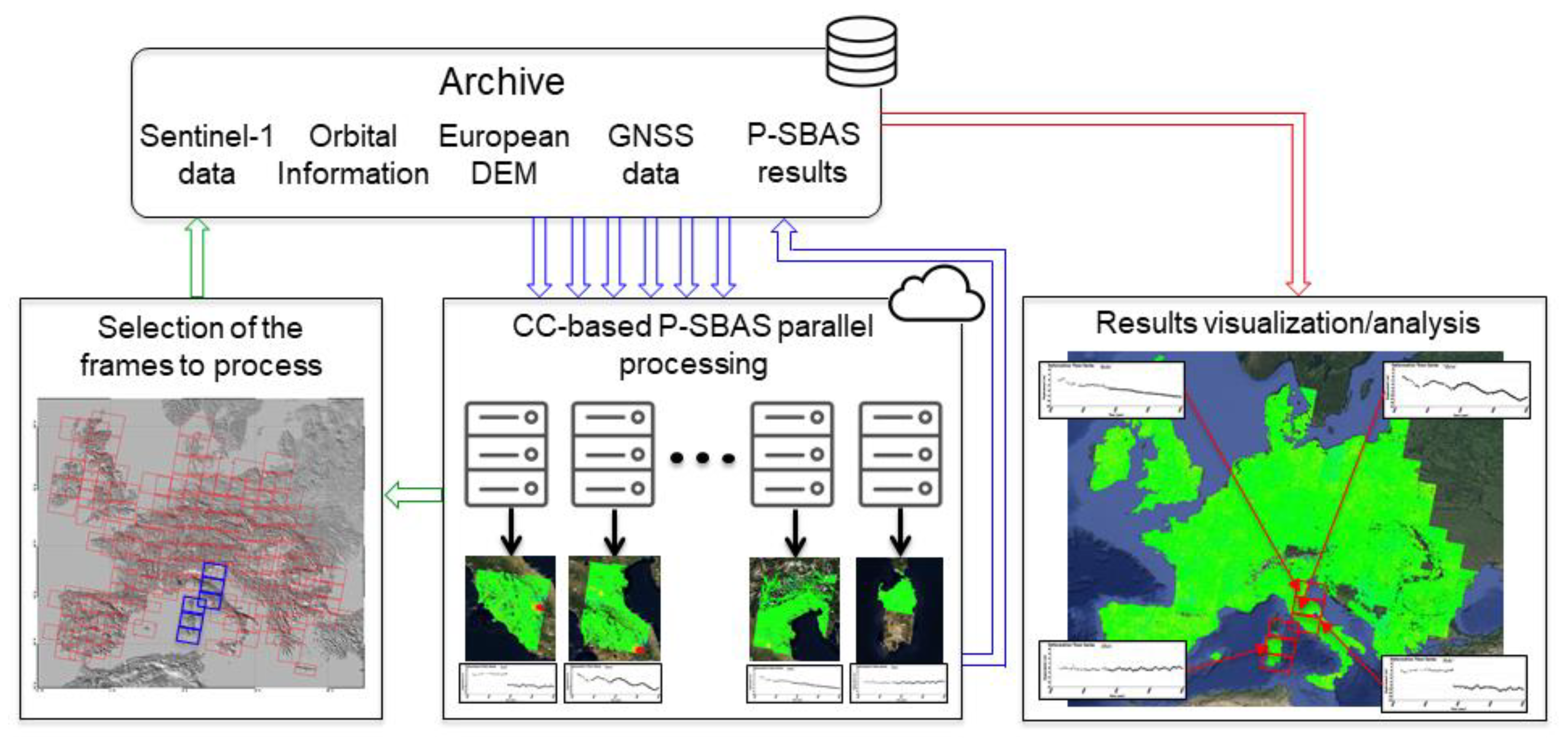
We present in this section a short overview of the exploited S-1 IWS P-SBAS processing chain, whose block diagram is sketched in Figure 1. Note that it represents a modified version of the one reported in [20], since we have introduced an additional step aimed at identifying and filtering out possible residual atmospheric artifacts that may affect the DInSAR measurements. This result is achieved through the proper exploitation of the available GNSS position time series, whose details are provided in the following section. Moreover, we have improved the automation and robustness of the S-1 P-SBAS processing chain from the algorithmic point of view by introducing several check mechanisms to guarantee its fully unsupervised execution.

In the following, we briefly describe the main blocks characterizing this approach and the basic rationale of its implementation in the exploited CC environment, without detailing the implemented algorithmic solutions and the parallelization techniques exploited for each processing step, which are extensively discussed in [19,20]. In this sense, it is worth noting that the black and blue colors used to outline the different blocks shown in Figure 1 allow us to easily discriminate the processing steps that are intrinsically sequential (black) from those where the concurrent jobs are executed in parallel (blue) by distributing the input data processing among different computing nodes. Among the latter, the steps that benefit from the aforementioned burst partitioning granularity, which represents a key element of the parallelization strategy of the exploited S-1 processing chain [19,20], are marked by red color texts.

In the first block of the diagram in Figure 1 (block A) we implement the operations for handling and ingesting the input data, represented by the sequence of S-1 single look complex (SLC) burst images, the orbital information associated to each SAR acquisition, the digital elevation model (DEM) of the investigated zone, and the GNSS position time series available for the area that, in our case, are provided by the Nevada Geodetic Laboratory at the University of Nevada, Reno, USA (UNR-NGL) [25].

Once the input data are correctly ingested, block B performs a series of sequential operations, comprising the selection of the reference SAR geometry for the registration of the entire SAR dataset, the identification of the area of interest, as well as of the burst images to be processed. Moreover, a first list of interferometric data pairs involving the available SAR acquisitions is created, which is then exploited within the subsequent interferograms generation and noise filtering operations [27].

Block C performs the conversion of the available DEM into the radar (azimuth and range) coordinates through the range Doppler equations [7], followed by the estimation, for each pixel of each SAR scene, of the range and azimuth distances with respect to the reference orbital position.

Block D concerns the co-registration of each burst image with respect to the reference acquisition, the burst interferogram generation, and subsequent correction to compensate the effects of possible residual azimuthal misregistration errors. Note also that a spatial multi-look operation is carried out to mitigate the decorrelation noise effects within the generated burst interferograms and to reduce the amount of data to process.

At this stage, in block E the corrected multi-look interferograms (and the corresponding spatial coherence maps) of adjacent bursts are accurately assembled through an interferogram mosaicking operation to generate the differential interferograms of the whole investigated area, which is hereafter referred to as “frame”. Moreover, on these interferograms, the noise filtering procedure discussed in [27] is applied.

Subsequently, a selection, among all the considered small baseline interferometric pairs, of an optimized triangular network within the perpendicular baseline/time plane is computed in block F [27]. In particular, regarding the temporal and spatial baselines, we select a maximum value of 150 days for the former and of 200 m for the latter. This implies that essentially no constraint is applied to the spatial baselines because the orbital tube diameter is about 200 m.

The sequence of the so-identified multi-look noise-filtered small baseline interferograms of the frame is then unwrapped through the extended minimum cost flow (EMCF) phase unwrapping (PhU) algorithm [28] (block G). Then, in block H, a first estimate of the deformation time series is retrieved by applying the SVD method, following the lines of the original SBAS approach [8]. This block also implements a procedure for the compensation of possible topographic phase residuals. Moreover, it includes the estimation and removal of atmospheric artifacts by taking into account that they are typically correlated in space and poorly in time [8], as well as by benefiting from their correlation with topography [29].

Block I represents an additional step implemented within the presented P-SBAS processing chain, which is discussed in details in the following section. In this block, the available GNSS measurements are used to identify and filter out possible residual atmospheric artifacts that may affect the DInSAR measurements [23,24].

Lastly, block J computes the final displacement time series and the corresponding mean deformation velocity map of the investigated frame, generated in a geographic/cartographic reference system.

Concerning the CC implementation of the S-1 IWS P-SBAS processing chain shown in Figure 1, and the corresponding job scheduling, we remark that they are carried out through a fully automatic pipeline able to exploit the available resources, which follows the lines of the solution presented in [19,20] and is sketched in Figure 2. In particular, it starts by downloading and unpacking the S-1 input data in parallel, from the input data archive, by ingesting as inputs the list of S-1 IWS SLC burst images relevant to the investigated frame, and identified by the vertexes of the area of interest to be analyzed. Then, it distributes the S-1 IWS data among the available computing nodes and manages their parallel processing by using both multi-node and multi-core programming techniques. We also stress that different parallelization strategies are adopted throughout several steps of the processing chain of Figure 1, depending on the implemented algorithm structure, as well as on the amount and the type of data they process and on the available computing resources required (RAM, I/O bandwidth, CPUs consumption, etc.) [18,21,22].

At the end of each processing, the developed pipeline performs the upload of the generated DInSAR results on the storage archive dedicated to their preservation. Moreover, as soon as the processing of one frame is completed on a computing node, it launches a new query to the archive in order to proceed with the next S-1 frame. The final results can be visualized and analyzed through appropriate GIS and WebGIS platforms [30].

The overall pipeline is written through a set of bash scripts, which allow exploiting any kind of Linux-based computing environment [19].

Moreover, we remark that in the context of massive DInSAR analyses an effective automation of the input data ingestion and efficient processing, and of the storing of the achieved results represents a crucial point to be addressed. Accordingly, in order to guarantee the fully unsupervised execution of the S-1 P-SBAS processing, we have introduced several check mechanisms at the algorithmic level to guarantee the robustness and the reliability of the pipeline.

In particular, once selected the area of interest relevant to the frame to be processed, there is a first algorithm check verifying that the selected burst images fully cover the selected area, thus avoiding gaps in the DInSAR coverage. Another check mechanism is implemented to investigate if an S-1 input data has been processed more than once with different IPF version [31] in order to select the more recent one. Additional checks are focused on automatically identifying the reference coherent pixel on each frame by also exploiting the available GNSS information or, if unavailable, the triangular coherence [20].

3. Joint Exploitation of GNSS and DInSAR Measurements

The GNSS measurements can provide three-dimensional information, with millimetre accuracy, on the ongoing deformations (East, North, and vertical components) through the accurate evaluation of the receiver stations position. However, the spatial distances among the GNSS stations are often too large to capture localized displacement patterns, while they are typically appropriate for the study of the low spatial frequency deformation fields, often due to regional (tectonic, in several cases) phenomena. On the other hand, the DInSAR techniques provide, for SAR data acquired from a single illumination geometry, one-dimensional surface deformation measurement along the radar Line of Sight (LOS), but with a wide spatial density; this peculiarity makes DInSAR an incomparable technology for reconstructing high spatial frequency deformation patterns. Accordingly, the joint use of GNSS and DInSAR technologies appears to be particularly effective for the retrieval of the deformation signals affecting a specific area of interest [23,24], and is even more important for continental scale analysis like the one presented in this work. Accordingly, this is the key task of the approach discussed in the following.

To clarify the basic rationale of the presented solution, let us first focus on the LOS DInSAR displacements, whose expression can be written as follows:

$$d_{LoS}= d_{HF}+d_{LF}+ {\eta }_{APS}+ {\eta }_{HF}+ {\eta }_{LF}$$

(1)

where $d_{HF}$ is the high spatial frequency deformation component due to localized deformation patterns (such as landslides, local subsidence, etc.), $d_{LF}$ represents the low spatial frequency deformation relevant to possible regional displacements, ${\eta }_{APS}$ is due to the tropospheric noise affecting the DInSAR signals, ${\eta }_{HF}$ accounts for high spatial frequency deformation effects due to PhU errors, i.e., $2\pi$ multiples that were wrongly estimated within the unwrapping operation of the interferometric phase [27,28], and ${\eta }_{LF}$ is relevant to low spatial frequency artefacts due to atmospheric residuals. It is worth noting that possible DEM errors have been estimated and compensated for in block H although, because the S-1 system is characterized by a very narrow orbital tube [20], the corresponding phase errors can be considered negligible and therefore they are not included in Equation (1). Starting from the $d_{LoS}$ measurements, we want to correctly retrieve the $d_{HF}$ and $d_{LF}$ signals in Equation (1).

Concerning the P-SBAS processing chain, we remark that it already includes methods for the PhU errors mitigation (factor ${\eta }_{HF}$, in Equation (1)) [32] and for the APS removal (factor ${\eta }_{APS}$, in Equation (1)) [8]. Accordingly, our main efforts have been focused on the mitigation of the impact of the factor ${\eta }_{LF}$ (see Equation (1)). In particular, the overall analysis is focused on the identification and removal of the mean rate of the signal component ${\eta }_{LF}$, which is referred hereinafter as $v_{{\eta }_{LF}}$, through the profitable exploitation of the low pass frequency deformation signals retrieved from the GNSS measurements. To do this, we have developed a rather simple solution, which is depicted in the block diagram of Figure 3 and discussed in detail as follows.

3.1. GNSS Data Screening and Selection

The starting point of our algorithm is a preliminary screening of the measurements accessible through the available GNSS stations. In particular, this allows the identification of the GNSS stations whose measurements can be effectively used to filter out the signal component $v_{{\eta }_{LF}}$.

To do this, as detailed in the following, it is essential to identify the stations whose signals are:

• Sufficiently extended in time (in our case at least 2 years) and “cleaned” of possible jumps and artefacts, which may affect the correct estimation of the mean deformation rate components;
• Affected by regional scale signals only, which are therefore spatially correlated and that do not account for high spatial frequency deformation signals (i.e., localized displacements).

To clarify the need of the above-mentioned data screening, we remark that the GNSS stations time series can sometimes be perturbed by the presence of gaps in the data acquisitions and by steps, which can be generated by different causes, both anthropogenic and natural. In particular, software modifications or physical changes of the antenna receiver, as well as the occurrence of a seismic event, are the main reasons for the presence of these steps within the time series that, unfortunately, are not always identified through the auxiliary files, where the dates in correspondence of these issues are highlighted.

Accordingly, our data screening step identifies first the stations whose signals have a significant temporal extension that, in our case, corresponds to at least two years. Then, from each of them we extract the time interval that, with respect to the presence of possible steps in the time series, is reliable concerning the evaluation of the mean rate component. Accordingly, the GNSS stations whose signals are not consistent with the above characteristics are rejected from the procedure.

In Figure 4, five examples of the GNSS stations time series selection are shown. In particular, the plots on the left side show the original time series (we consider the East/West component as provided by the UNR-NGL web-site (http://geodesy.unr.edu)), while on the right, the corresponding ones following the automatic data screening procedure, are represented. Note that the plots 1 and 2 are representative of GNSS stations affected by seismic events: in particular, these two stations show the steps due to the 2016 Central Italy seismic sequence (24 August 2016, 30 October 2016, and 18 January 2017). Plots 3 and 4 outline some anthropic operations performed on the GNSS stations, which in some cases corrupts the GNSS station deformation rate estimation. Finally, we show that plot 5, although not supported by the auxiliary information, is filtered by the algorithm, which identifies the large temporal gap in the data and rejects the shorter part of the available time series, thus allowing a proper mean deformation rate estimation.

At this stage, the implemented procedure identifies the GNSS stations affected by regional signals only. To do this we exclude the GNSS stations characterized by a significant vertical deformation velocity (greater than 0.5 cm/year), because this is not consistent with long-term regional deformation signals and we take advantage of the strong spatial correlation of these phenomena, whose planar component velocities are spatially correlated for tens of squared kilometres [33]. In particular, we evaluate a similarity rate index of the GNSS stations that fall within a specific spatial window that in our case is empirically set to ~30 × 30 km². This similarity index, which we estimate for each GNSS station, is expressed as follows:

$$R_i= \frac{1}{n-1}{\displaystyle \sum }_{j=1}^{n-1}\left[\frac{v_i{v}_j}{v_i{}^2}\right]=\frac{1}{n-1}{\displaystyle \sum }_{j=1}^{n-1}\left[\frac{v_j}{v_i}\right]$$

(2)

where n represents the total number of the GNSS stations that fall within the above-mentioned spatial window, $v$ is the GNSS mean displacement rate, while i is the station where we are calculating the similarity index, and j is the index relevant to the remaining n × 1 stations that we compare with i. The spatial similarity rate index is designed to be equal to 1 when the deformation velocities of the stations falling within the spatial window are the same, while the similarity becomes worse for values of this index that move away from 1.

The evaluation of the similarity index in Equation (2) is typically carried out only on the planar components of the GNSS-based estimate of the mean deformation rate, which are expressed as follows for the ith GNSS station:

$$R_{e{w}_i}= \frac{1}{n-1}{\displaystyle \sum }_{j=1}^{n-1}\left[\frac{v_{e{w}_i}{v}_{e{w}_j}}{v_{e{w}_i}{}^2}\right]=\frac{1}{n-1}{\displaystyle \sum }_{j=1}^{n-1}\left[\frac{v_{e{w}_j}}{v_{e{w}_i}}\right]$$

(3)

$$R_{n{s}_i}= \frac{1}{n-1}{\displaystyle \sum }_{j=1}^{n-1}\left[\frac{v_{n{s}_i}{v}_{n{s}_j}}{v_{n{s}_i}{}^2}\right]=\frac{1}{n-1}{\displaystyle \sum }_{j=1}^{n-1}\left[\frac{v_{n{s}_j}}{v_{n{s}_i}}\right]$$

(4)

In particular, only the GNSS stations for which $\left(R_{e{w}_i},R_{n{s}_i}\right) \in \left[0.95, 1.05\right]$ are considered, within the DInSAR deformation signals refinement step discussed in the following paragraph.

In Figure 5, we represent the planar components (East-West and North-South) of the GNSS stations of the NGL catalogue, located in the entire European territory under investigation in this work. It is evident from the visual inspection of Figure 5 that the stations selected for our processing are highly spatially correlated and with no evident singularities present.

3.2. DInSAR Deformation Signals Refinement

In this paragraph, we describe the last steps of our procedure for the refinement of the DInSAR deformation signals relevant to each investigated SAR frame. In particular, this procedure aims to identify and remove possible low spatial frequency displacements artefacts, mainly due to residual atmospheric phase errors.

In Figure 6, we show a panel describing, step by step, the implemented procedure applied to the P-SBAS results generated for a selected frame that is relevant to a large portion of the Central-Northern Italy regions, included in the processing experiment presented in Section 5. Note that we select this frame because it is affected by different displacement phenomena, thus highlighting the efficacy of the implemented algorithm. In particular, the included Po Valley is historically affected by intense subsidence phenomena, as well as the city of Bologna [34]. Moreover, in the same frame we can appreciate the well-known displacements relevant to the Firenze–Prato–Pistoia basin [35,36], the subsidence phenomena affecting the Northern Adriatic Sea coastline [37], and in the South-East corner of the frame the impact of the August–October 2016 seismic sequence [38,39].

Figure 6A shows the starting point for the developed procedure. In particular it represents the mean displacement velocity map obtained from the original P-SBAS approach (see block H in Figure 1). Figure 6B depicts the low spatial frequency deformation pattern retrieved from the interpolation (Kriging interpolation [40]) of the GNSS stations planar displacement velocities projected along the satellite radar LOS. Clearly, for this step, we exploit only the GNSS stations returned by the screening operation and for values of the similarity rate index close to 1, as described in Section 3.1.

The mean deformation velocity retrieved by subtracting the GNSS-derived regional deformation pattern (Figure 6B) from the starting velocity (Figure 6A) corresponds to the input for the velocity calibration procedure. Such a procedure is equivalent to apply a simple low pass spatial filter for the estimation and removal of possible artefacts. Figure 6C shows the result of the calibration step that allows us to correct the retrieved deformation signals.

At this stage, to reconstruct the overall displacement field affecting the area of interest, we can add the low and high spatial frequency deformation components (Figure 6B,C, respectively). The mean deformation velocity map corresponding to the final result is shown in Figure 6D. Moreover, the above-described procedure is also graphically summarized with a block diagram at the bottom of Figure 6.

As an additional remark, we underscore that both results shown in Figure 6C,D can be separately exploited for different scientific purposes, thus increasing the range of the value-added results offered by these advanced DInSAR analyses.

We finally present the results of the comparison between the refined DInSAR deformation time series and those of the available GNSS stations relevant to the frame of Figure 6. Obviously, we exploit in this comparison only the GNSS stations that have not been accounted within the DInSAR signals refinement step.

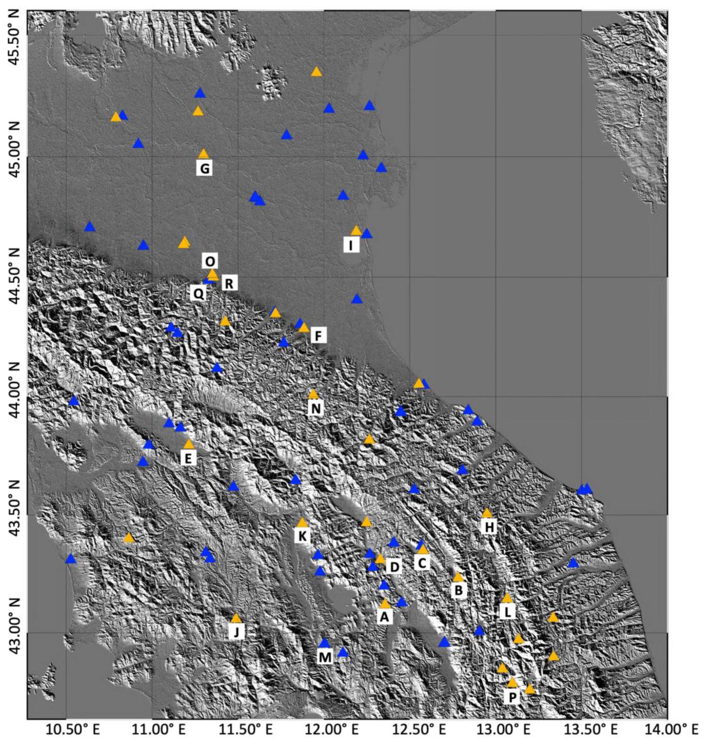
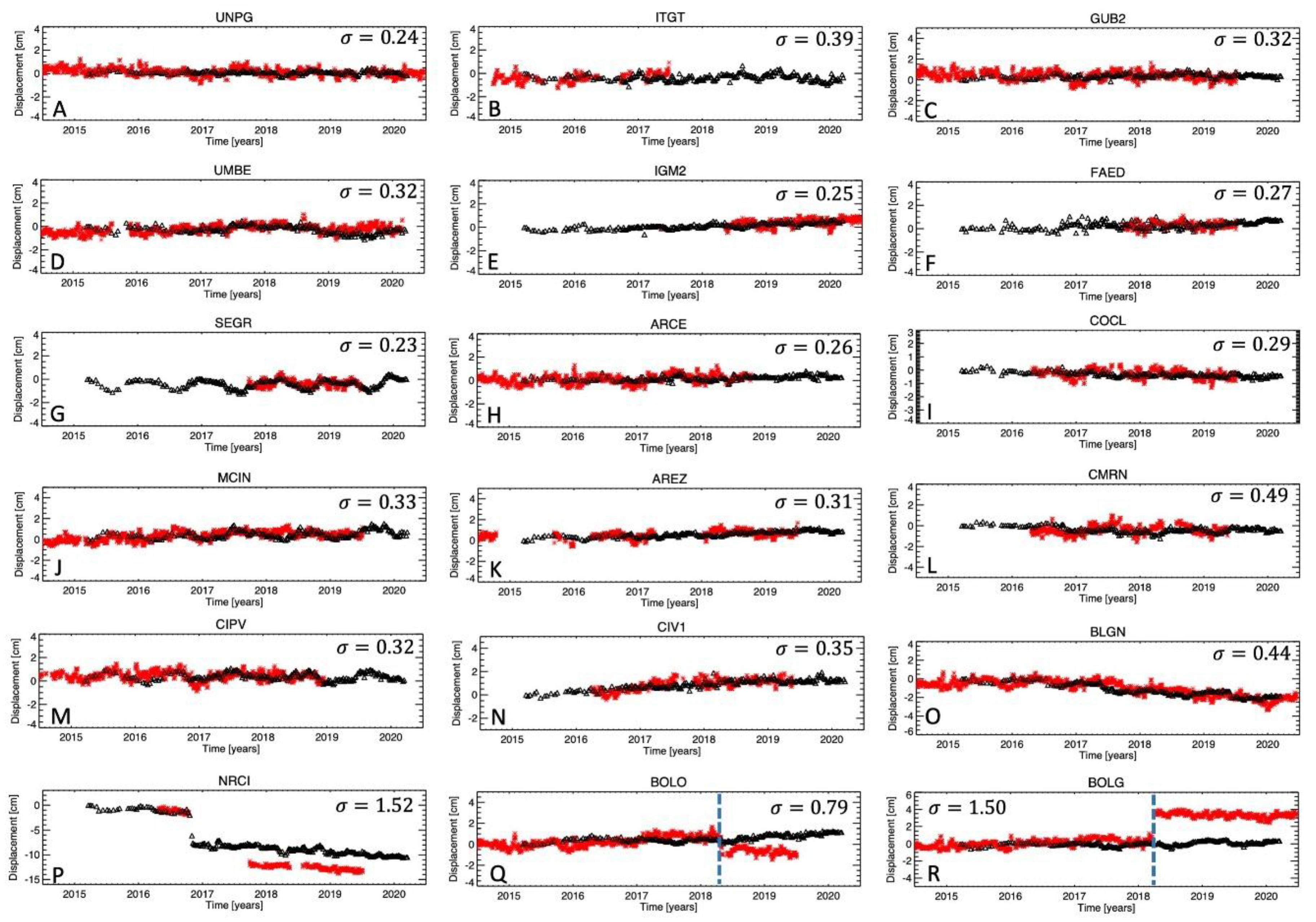
In Figure 7 we show the DEM of the area, highlighting the sites of all the GNSS stations that have been investigated in our study; they are identified by blue and yellow triangles, representing the stations exploited for and excluded from the DInSAR deformation signals refinement step, respectively. In Figure 8, we report a selection of plots showing the comparisons between the deformation time series retrieved through the developed S-1 IWS P-SBAS processing pipeline (black triangles) and the corresponding LOS-projected GNSS ones (red stars) for the stations labelled in Figure 7 with capital letters from A to R. We remark that, since the GNSS time series themselves are affected by noise (although they are assumed as reference), we considered a smoothed version of the GNSS time series in our comparative analysis.

Figure 8A–O show the plots relevant to some GNSS stations that were excluded from the DInSAR deformation signals refinement procedure. The good agreement between the P-SBAS and LOS-projected GNSS measurements is evident, as also testified by the standard deviation values of the difference between the two time series, computed in the temporal window common to both measurements, ranging from 0.23 and 0.49 cm. Moreover, we also show in Figure 8P–R the plots for three GNSS stations where, for different reasons, the performed comparison is not satisfactory. In particular, Figure 8P is relevant to a GNSS station located in the area that was strongly struck by the 2016 Central Italy seismic sequence. In this case, the discontinuity characterizing the DInSAR time series in correspondence to the earthquake is clearly underestimated due to PhU errors [41,42]. In addition, Figure 8Q,R present the plots of two GNSS stations where the effects of the antenna code changes, as reported in the GNSS auxiliary files, are evident.

4. Exploited SAR and GNSS Data and Cloud Computing Resources

We describe in this section the input SAR and GNSS data we exploit in this study. Moreover, we briefly describe also the cloud computing resources and architecture we use to perform the whole P-SBAS processing.

4.1. SAR and GNSS Data

As stated already, the SAR images we analyze have been acquired by the Sentinel-1A and Sentinel-1B satellites. The overall investigated area has been divided in 175 frames, from 21 descending orbit tracks, with an average size of almost 200 × 250 km (azimuth and range, respectively). An overlap between frames has been preserved, covering almost 20% of the frame size for two subsequent ones in the azimuth direction. This overlapping area allows us to perform consistency tests on the analyzed zone, in order to guarantee an additional check for the continuity preservation of the achieved result. In Figure 9, we show the footprint of the 175 S-1 frames processed in this study.

The time series of every frame have been retrieved by using data acquired from March 2015 to September 2018 with the average number of SAR images for each frame varying between 400 and 450, depending on the different regions. Moreover, for the frames relevant to Italy, our analysis has been extended to March 2020, since this study also supports a project led by the Italian Ministry of Economic Development aimed at investigating the deformation phenomena affecting the Italian territory.

Globally we have used almost 72,000 SAR images covering a whole area of about 4,500,000 km², including the overlap among the considered frames.

Concerning the GNSS stations, we have used, as previously mentioned, the data provided by UNR-NGL [25] in the framework of the “Plug and Play GPS” project that takes the raw GNSS data from more than 17,000 stations all around the world and makes publicly available via a web-site (http://geodesy.unr.edu) the data products (including metadata, plots of position coordinates, etc.) for all the geodetic quality GNSS stations. The starting number of GNSS stations, whose data have been downloaded and analyzed in this study, is 4227. Following the data screening and selection procedure described in Section 3, we have exploited 2477 stations relevant to the investigated area. In Figure 10, we show the position of the stations: blue markers represent the stations used after the screening, while the yellow ones represent the stations whose data have been neglected because they are considered unsuitable for the implemented DInSAR deformation signals refinement operation.

4.2. Cloud Computing Resources

As anticipated before, we perform the CC implementation of the S-1 IWS P-SBAS processing pipeline discussed in Section 2, by exploiting the computing resources provided by the ONDA DIAS CC platform [26]. In particular, we use six computing nodes, each one equipped according to the characteristics reported in

Table 1. ONDA DIAS Computing Nodes Configuration.

ONDA DIAS Computing Nodes Configuration
Architecture	64 bit
vCPU/vCores *	64
RAM	512 GB
Internal Disks	18.5 TB (5 SSD in RAID 0 configuration)
Network	2 Gb/s

* vCPU and vCores are acronyms of virtual CPU and virtual Cores, respectively.

. Note that the six nodes are connected to the S-1 IWS data archive, which is located on an object storage, via NFS with a guaranteed download bandwidth of 2 Gb/sec (see Figure 11). As mentioned, having the data archive close to the computing resources and accessible through a dedicated and fast connection is a key requirement when the processing of such a huge data volume is envisaged, because of the data transfer overhead. In this framework we also remark that we fully benefit from the specific APIs made available by ONDA in order to effectively and automatically perform the S-1 images query and download operations.

5. Experimental Results

We processed through the CC-based S-1 P-SBAS pipeline described in Section 2 the S-1 IWS data-set acquired over the wide portion of the European territory detailed in Section 4.1. As stated before, the data-set considered is composed of 175 frames (see Figure 9) and for each of these, the selected SAR image temporal sequences were individually processed. We remark that no spatial baseline constraint was imposed in the interferometric pair selection exploited in our processing thanks to the narrow orbital tube characterizing the S-1 constellation [20]. Moreover, we exploited the 1-arcsec SRTM DEM to generate the analyzed DInSAR interferograms on which we performed a complex multi-look operation with twenty looks in the range direction and five looks in the azimuth one, thus obtaining a pixel dimension of about 80 × 80 m. The same DEM was also used to geocode the computed deformation time series and the corresponding mean velocity maps.

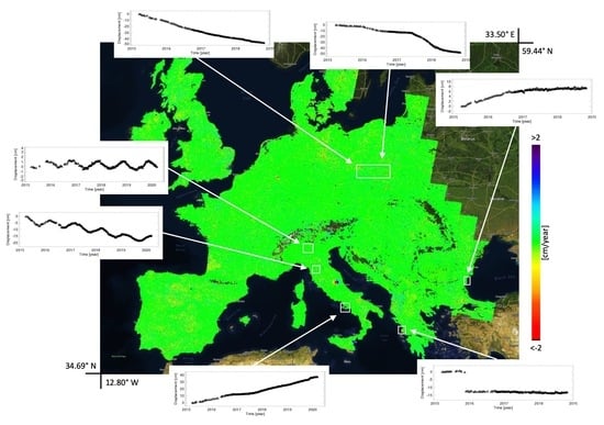
In Figure 12 we present the mosaicking of the obtained mean deformation velocity maps of the overall investigated area, geocoded and superimposed on an optical image. The displayed overall mean velocity map provides information on the ongoing deformation mean values of the coherent pixels, identified by considering those with a temporal coherence value [28] greater than a selected threshold that in our analysis is set equal to 0.9 for all the analyzed data-sets. Overall, we detect ~120,000,000 coherent pixels for which the corresponding deformation time series are available. Moreover, the zones exhibiting lower temporal coherence values are properly masked out. The velocity maps in Figure 12 show a large variety of localized deformation patterns due to different phenomena (volcanic activities, earthquakes, subsidence phenomena, slope instabilities, man-made activities, etc.), with the most evident one being the well-known deformation pattern associated with the seismic crisis that struck Central Italy during the August–October 2016 period, already extensively discussed in [38,39].

Starting from the results of Figure 12, and to provide a clearer idea about the generated products, we present in the following the zoom-in views of the mean deformation velocity map relevant to six areas characterized by significant ground displacements related to natural phenomena (Figure 13, Figure 14 and Figure 15) and man-induced activities (Figure 16, Figure 17 and Figure 18), which are outlined by white rectangles. Moreover, for each area, we show the plots of the deformation time series of some selected coherent pixels.

In particular, in Figure 13a, we show the zoom-in view of the mean deformation velocity map portion relevant to the Campi Flegrei caldera (Southern Italy), an active volcanic area located West of the city of Napoli. It is characterized by the bradyseism phenomenon consisting in a slow lifting and lowering movement of the ground; since late 2005 [43,44,45,46,47] the caldera has been experiencing an almost continuous uplift of the ground surface. Indeed, the map in Figure 13a shows a spatially extended deformation pattern involving the whole caldera with a maximum LOS deformation rate of about 7.5 cm/year. We also present the plot (Figure 13b) of the displacement time series of a pixel located in the maximum deformation area, identified by a white star and labeled as P1 in Figure 13a, characterized by a cumulative displacement of about 37 cm. The temporal evolution of the displacement for the selected pixel shows the deformation behavior characterizing the caldera since 2015. As a matter of fact, we observe a rather continuous uplift typified by different deformation rates within the whole period of observation. In addition, a decrease of the deformation rate, approximately spanning from mid-2016 to mid-2017, is also clearly visible. Finally, in Figure 13c, we report the mean deformation velocity values for the coherent pixels deployed along the section crossing the maximum uplifting zone and identified in Figure 13a by a dashed white line. It is evident that the caldera shows a general uplift characterized by an almost radial symmetry with respect to the maximum displacement located in the Rione Terra area (P1 in Figure 13a).

In Figure 14a, we highlight a sketch of the mean deformation velocity map relevant to the Lefkada Island (Greece). It outlines a spatially extended deformation pattern, characterized by both negative and positive LOS-projected displacement signals, which are related to the Mw 6.5 earthquake that struck the island the 17 November 2015 [48,49]. Moreover, we present the corresponding displacement time series relevant to two selected pixels (labeled as P1 and P2 in Figure 14a and marked by white stars) located in the maximum co-seismic deformation zone. They clearly show the deformation signal associated with the seismic event, see the discontinuity characterizing the time series of Figure 14b,c in correspondence to the earthquake (highlighted by a vertical dashed red line).

In Figure 15, we show a zoomed-in view of the mean deformation velocity map relevant to the Northern Black Sea coast, between the Varna and Kavarna towns (Bulgaria). This area is characterized by numerous landslides, mainly due to soil over-moistening, marine erosion, slope cutting and seismic impacts, which have caused serious damage to buildings and infrastructure over time [50]. Figure 15a reports the LOS mean deformation velocity map of the area while Figure 15b,c display the corresponding displacement time series relevant to two selected pixels (labeled as P1 and P2 in Figure 15a and marked by white stars), located in Balchik town and in Kranevo village (both between Varna city and Kavarna town), respectively. These plots clearly show the ground movements, characterized by different rates (about 1 and 1.8 cm/year for P1 and P2, respectively), related to the landslides.

Moving from the ground deformation analysis related to natural phenomena to human-induced activities, we benefit first from the DInSAR capability to investigate displacements caused by mining activities [51,52]. In particular, we show in Figure 16a,b two zooms of the map of Figure 12 relevant to rather wide zones located in Germany (a) and Poland (b), respectively, where significant mining activities are carried out. In Figure 16c, we report a zoomed-in view in correspondence to the Nochten coalmine and surroundings, located in the Saxony-Anhalt State (Germany), where the effects of the sub-surface exploitation activities on the ground deformation are evident. In addition, we show in Figure 16e the displacement time series relevant to a selected pixel (labeled as P1 in Figure 16c and marked by a white star) that reveals cumulative displacements of more than 45 cm in the considered time period. Similarly, in Figure 16d we show a zoomed-in view of the Katowice coalmines, located in the Silesian Region (Southern Poland). As for the German case, the ground deformation related to mining actions are clear. The plot of the displacement time series (see Figure 16f) relevant to a selected pixel (labeled as P2 in Figure 16d and marked by a white star) located in the area shows a clear non-linear deformation behavior, which is effectively retrieved through our P-SBAS-based analysis.

We remark that, following the deformation time series retrieval operation, the S-1 IWS P-SBAS processing chain automatically supplies various value-added information on the ongoing deformation phenomena. Indeed, in addition to the estimate of the mean deformation velocity, it also automatically identifies possible deformation signals characterized by a periodic behavior with respect to time, such as those relevant to oil and gas extraction/storage activities and water withdrawal, which represent significant DInSAR applications in the energy source storage [53] and hydrogeological [54] fields. This is done by computing the correlation coefficient of each pixel’s detrended time series with a sinusoid with a one-year period. In Figure 17a we show the peak-to-peak amplitude of the sinusoid signal in an area located in Northern Italy, close to the city of Milano. Note that pixels with peak-to-peak amplitude values equal to 0 are those for which the correlation coefficient is smaller than 0.8. The oscillation amplitude map clearly identifies three distinct areas that correspond to three gas storage sites located in the zone. In Figure 17b,c we show the displacement time series relevant to three selected pixels, labeled as P1, P2, and P3 in Figure 17a and marked by black stars, located in correspondence to the Settala, Sergnano, and Ripalta Guerina sites, respectively. The displayed time series reveal periodic deformation signals that correspond to the human-induced actions carried out to ensure gas supply during the winter. Indeed, the plots clearly show the effect of the injection of gas into storage during periods of low demand (approximately from March to October), which produces a raising of the soil over the reservoir area. Conversely, it is evident that a subsidence effect during periods of peak demand (approximately from November to February) occurs due to the withdrawal of gas migration from storage into the town’s gas supply system. As a further example of this kind of analysis, we show in Figure 18 the oscillation amplitude map relevant to the Firenze-Prato-Pistoia basin (North Italy). In this case, the displacement time series relevant to a selected pixel (labeled as P1 in Figure 18a and marked by a black star) shows a clear subsidence signal, caused by the large amount of ground-water extracted due to the industrial activities carried out in this area [35,36]. Moreover, this subsidence trend is modulated by a seasonal oscillation, due to the groundwater withdrawal and recharge during the summer and winter seasons respectively, see Figure 18b.

It is also worth noting that the two examples reported in Figure 17 and Figure 18 identify deformation signals characterized by oscillations that peak in different periods: approximately in November for the first case and February for the second one. This temporal peak location is a key parameter to discriminate the occurrence of such different displacement phenomena.

6. Conclusions

The amount and availability of remote sensing satellite data have exponentially grown in recent years, significantly contributing to the on-going big data scenario. In particular, a key role is played by the Copernicus program of the European Union through the Sentinel missions, characterized by its free and open data policy [55]. In this framework, the wide spatial footprint, the high temporal acquisition rate, the accurate synchronization among subsequent acquisitions, the selection of a unique acquisition mode over land, and the accurate orbital information with a small tube diameter, which characterizes the Sentinel-1 constellation [1], have already represented a revolution for the possibility to operationally apply the DInSAR techniques to investigate Earth surface deformation phenomena at unprecedented spatial and/or temporal scales. In this paper, we present a CC-based solution to perform, through the P-SBAS processing chain, advanced DInSAR analyses from S-1 IWS SAR images and GNSS position time series at continental scale in an automatic, efficient, and robust way.

To achieve such a task, processing and storing huge data flows, including GNSS, DEM, and orbital information, in addition to very large S-1 IWS SAR data volumes, are required. To do this, there is a need, on the one hand, for proper DInSAR processing algorithms and, on the other hand, for appropriate computing architectures, wide storage capacity, and high performance processing resources. In this framework, key problems to be addressed are also those relevant to the automation level and the reliability of the entire processing strategy. Indeed, carrying out continental scale DInSAR analyses results in the ability to process large volumes of SAR data, preventing algorithmic errors, processing and computing failures, and hardware faults as much as possible.

From the algorithmic point of view the developed S-1 IWS P-SBAS processing chain has been enriched with a processing step that, starting from the available GNSS measurements, following a proper screening and selection operation, allows identifying and filtering out possible residual atmospheric artifacts that may affect the DInSAR measurements, thus generating refined DInSAR products (see Section 3). Moreover, regarding the automation and the robustness of the processing chain and of the relevant CC-based pipeline, several check mechanisms have been introduced in order to guarantee a fully unsupervised processing execution, as thoroughly discussed in Section 2.

With respect to the architectural issues, the main aspects impacting the efficiency of the S-1 P-SBAS pipeline are: i) proximity of data to the HPC infrastructure, ii) large storage capacity, and iii) wide computing capability in order to handle the requested massive parallel computation. Therefore, cloud computing, whose main characteristics are high availability, reliability, and robustness, has revealed as a natural choice to implement the presented continental scale S-1 IWS P-SBAS processing pipeline. In this case, we have successfully demonstrated that the European DIAS Cloud Services, in particular the exploited ONDA Cloud Platform, are suitable to host our fully automated pipeline for downloading and processing the analyzed S-1 images, and for storing the final S-1 interferometric products.

We further remark that, through our processing experiment, we have also successfully verified the high reliability and compliance with respect to the defined formats of the S-1 images archives, which represents another very relevant element supporting the possibility to operationally carrying out such massive DInSAR data processing.

The presented results, obtained through an extensive experimental analysis on a large portion of Europe (see Section 5), clearly show that the implemented CC-based S-1 P-SBAS pipeline has proved to be successfully suitable for massive and automatic continental scale DInSAR processing, which has been completed in six months and at relatively low computing costs amounting to about € 60k. In particular, the presented pipeline allowed the production, for the presented experiment, of the deformation time series and the corresponding velocity maps relevant to each single frame in six days, on average. Nevertheless, we underline that possible improvements of the proposed solution can already be envisioned. For instance, we report that an enhancement for improving the storage connection and performance could be very valuable. In addition to the above consideration, we remark that although the presented analysis has been carried out by exploiting averaged (multi-look) interferograms, it can be efficiently extended to the full resolution spatial scale by using graphics processing units (GPUs), following the lines of the approach presented in [56]. Moreover, algorithmic improvements concerning the compensation of residual phase unwrapping errors [32] and the integration of atmospheric information [57] for improving the tropospheric artifacts removal can also be very important.

Generating updatable interferometric products at a continental scale provides the possibility to access an unprecedented amount of results containing value-added information that is potentially groundbreaking. For instance, an extensive analysis on the interferometric coherence, performed on a country by country basis for land cover classification and mapping, or vegetation density detection, or the study of the statistics of the retrieved DInSAR deformation time series (for instance, standard deviation or root mean square values) and of their correlation with specific (linear, logarithmic, exponential, periodic, etc.) signals, to identify different deformation phenomena or potential changes that occurred during the observation period, could represent very relevant issues. Moreover, the availability of spatially dense deformation time series over such large areas paves the way to new kind of analyses and interpretation of such data. For instance, the idea of applying machine and deep learning techniques [58,59] to follow the behavior of deformation signals and to automatically extract significant patterns is becoming a very relevant issue but other innovative methodologies could be devised for deeply exploiting these “new generation” sources of DInSAR measurements.

As a final remark, we underline that the results we achieved can be particularly relevant for the Solid Earth community that promoted this experiment as a key study of the EPOSAR service included in the Satellite Data Thematic Core Service of the European Plate Observing System (EPOS) (https://www.epos-ip.org/). Moreover, our findings may also have a positive impact on the future development of the European Ground Motion Service [60], which is expected to start in the near future.