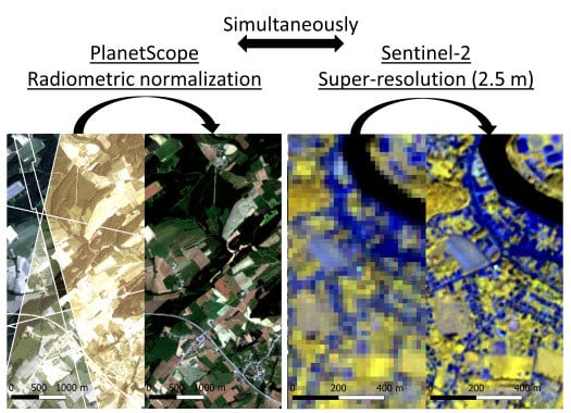
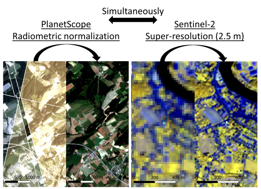
PlanetScope Radiometric Normalization and Sentinel-2 Super-Resolution (2.5 m): A Straightforward Spectral-Spatial Fusion of Multi-Satellite Multi-Sensor Images Using Residual Convolutional Neural Networks

Abstract

Sentinel-2 (S2) imagery is used in many research areas and for diverse applications. Its spectral resolution and quality are high but its spatial resolutions, of at most 10 m, is not sufficient for fine scale analysis. A novel method was thus proposed to super-resolve S2 imagery to 2.5 m. For a given S2 tile, the 10 S2 bands (four at 10 m and six at 20 m) were fused with additional images acquired at higher spatial resolution by the PlanetScope (PS) constellation. The radiometric inconsistencies between PS microsatellites were normalized. Radiometric normalization and super-resolution were achieved simultaneously using state-of–the-art super-resolution residual convolutional neural networks adapted to the particularities of S2 and PS imageries (including masks of clouds and shadows). The method is described in detail, from image selection and downloading to neural network architecture, training, and prediction. The quality was thoroughly assessed visually (photointerpretation) and quantitatively, confirming that the proposed method is highly spatially and spectrally accurate. The method is also robust and can be applied to S2 images acquired worldwide at any date.

1. Introduction

Satellite imagery provides a unique and detailed perspective on the state and changes in land, coastal, and oceanic ecosystems [1]. However, extractible information is limited by the spectral, spatial, and temporal resolutions of remote sensing images. Due to trade-offs in satellite instruments, images have generally either a high spatial resolution and a low spectral resolution or vice versa. One of the most used solutions is pansharpening: the fusion of a multispectral (MS) image with a panchromatic (PAN) image, both acquired simultaneously by the same satellite and capturing the same area [2]. MS images are typically composed of several bands partitioning the solar radiation into different spectra (e.g., red, blue, green and near-infrared). PAN images are composed of one band but capturing the whole solar radiation at a higher spatial resolution than MS images. The resulting pansharpened image combines the highest spatial resolution of PAN image with the highest spectral resolution of MS image. The numerous available pansharpening methods can be labeled as spectral, spatial, and spectral-spatial or spatiotemporal [3].

Pansharpening is a special case of image fusion: a combination of several images into a single composite image that has a higher information content than any of the original images [4,5]. Image fusion can thus also be done with images acquired at different dates/times by multiple sensors (optical, radar, hyperspectral, thermal, etc.) and embedded in different platforms (multiple satellites possibly in combination with other aerial vehicles). In that case, most of the traditional methods used for pansharpening (with MS and PAN images) cannot be applied [2,6]. The numerous studies focusing on fusion of remote sensing images have proposed various methods, each one adapted to the image characteristics and aiming at predefined objectives [4,5,7].

These last years, deep learning, and in particular neural networks (NNs), has been extensively used in the remote sensing community, mainly for classification and object detection but also, to a lesser extent, for image fusion [8]. NNs provide a flexible and powerful way to approximate complex nonlinear relationships without a priori assumptions on variables’ relationships. The network architecture can be multi-dimensional, thus potentially including spectral, spatial, and temporal variabilities within and between images. Deep convolutional neural networks (CNNs) are the most popular for image analysis due to excellent performances and proved efficiency [9]. CNNs are robust thank to their particular architecture characterized by local receptive fields, shared weights, and subsampling. Many studies have implemented pansharpening and single sensor image fusion using CNNs with very concluding results [6,9,10,11,12]. This study focused on image fusion from multiple sensors [4,13] with the goal to achieve super-resolution, i.e., further increasing the highest native spatial resolution [14]. For multi-sensor image fusion, Shao et al. [15] showed that previous methods, such as STARFM [16], ESTARFM [17], or ATPRK [18], were outperformed by CNNs.

Sentinel-2 (S2) imagery (European Space Agency) is composed of 13 bands at different spatial resolutions: four bands at 10 m, six bands at 20 m, and three bands at 60 m. The spectral resolution is high, but the spatial resolutions are not sufficient for fine-scale analysis. Higher spatial resolutions (such as 2.5 m) allow accurate geometrical analysis of small objects and finer descriptions and change detections in many areas [19,20]. To increase S2 spatial resolutions, several studies [21,22,23,24,25,26,27,28] have proposed to fuse the S2 bands together to super-resolve the coarser bands (20 or 60 m) to 10 m. However, these fusion methods cannot be used to further increase the resolution (e.g., 2.5 m), as S2 images at such resolution simply do not exist. A solution consists in using an additional source of images from a different satellite constellation. The red (B4), green (B3), and blue (B2) bands of S2 at 10 m were super-resolved to 5 m using the corresponding bands of RapidEye (Planet Labs) images [29]. Contrary to fusion methods using images from a unique satellite, this solution is more complex to implement because of differences in image footprint (swath) and acquisition date/time [29,30].

One of the additional sources of images could be the PlanetScope (PS) constellation (Planet Labs; planet.com) composed of more than 150 “Dove” microsatellites. These satellites cover the whole Earth at 3 m every day (about five days for S2). While superior in terms of spatiotemporal resolution, the radiometric quality is not equivalent to that of larger conventional satellites. Radiometric inconsistencies between different microsatellites was highlighted repeatedly [31], notably due to sensor-specific spectral response functions but also to variations in orbital configuration [32]. Several methods for radiometric normalization of PS imagery were thus recently developed using images of other satellite constellations, such as MODIS and Landsat [31,32,33], but not yet using the Sentinel-2 imagery.

In this paper, we present an innovative method aiming at simultaneously normalizing PlanetScope radiometry (all bands: R, G, B, and NIR) and super-resolving Sentinel-2 imagery (10 bands from 10 or 20 to 2.5 m) using deep residual convolutional neural networks. After a complete and detailed description of the method, the super-resolution quality was thoroughly assessed visually (photointerpretation) and quantitatively. The proposed method is highly spatially and spectrally accurate. Its robustness was illustrated for six locations around the world with contrasted acquisition conditions.

2. Materials and Methods

2.1. Software and Hardware

Preparation and processing of images and patches, as well as neural networks (NNs), were operated in R [34] with mainly three R packages: raster [35], sf [36], and keras (TensorFlow backend) [37], and in connection (command lines) with GDAL/OGR library [38] and Orfeo ToolBox [39,40]. Only one computer was used with satisfactory performance: Windows 10 64 bits, 64 Gb of RAM, 20 cores at 3.31 GHz, a 2 TB SSD, and a NVIDIA GeForce RTX 2080 graphic card (CUDA).

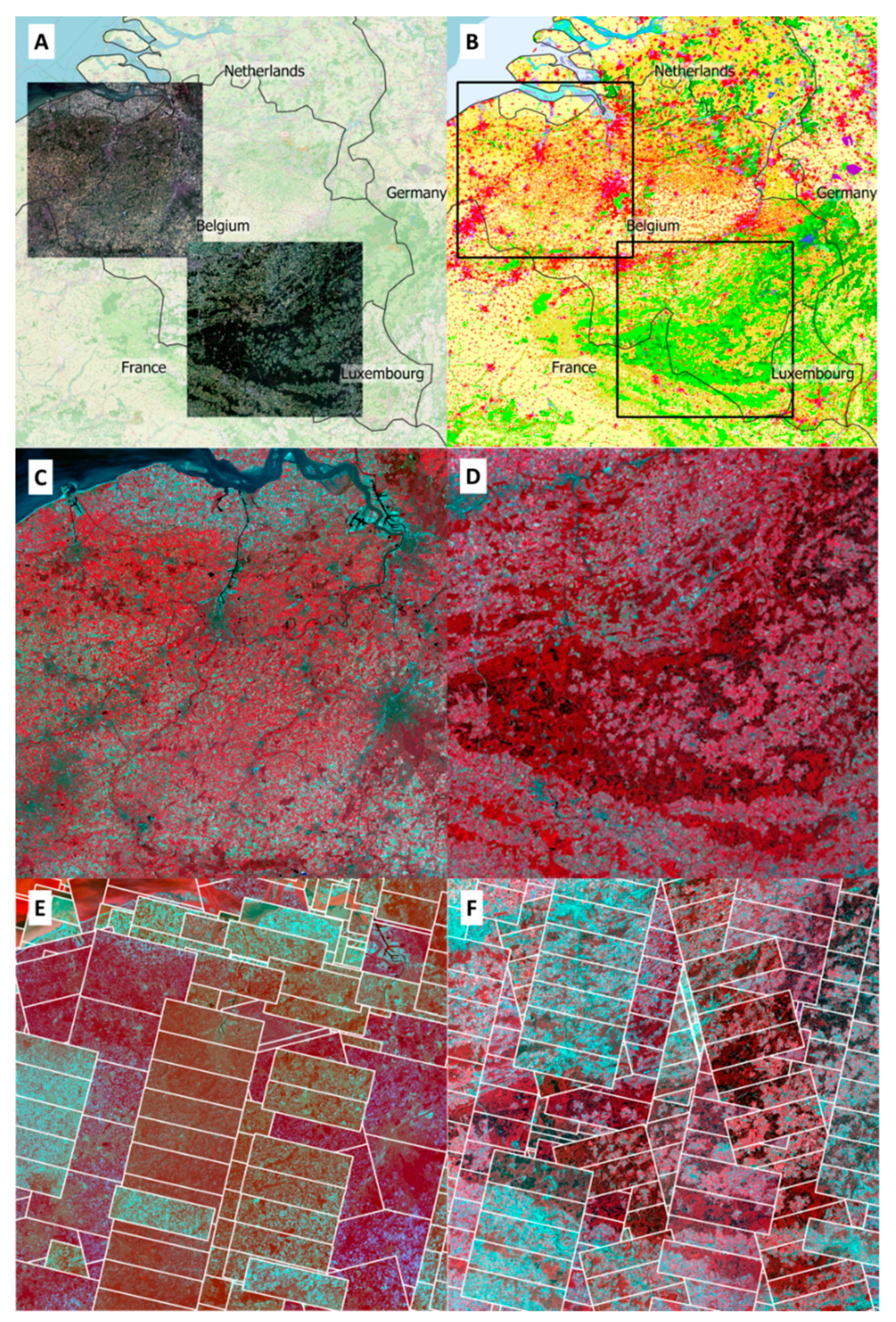
2.2. Image Selection

For both constellations, Sentinel-2 (S2) and PlanetScope (PS), images with the higher processing levels, i.e., bottom of atmosphere (BOA) surface reflectance, were selected: Level 2A for S2 and Level 3B (Analytic Ortho Scene) for PS. For S2, the 4 bands at 10 m and the 6 bands at 20 m were used. For PS, all the available bands (R, G, B, and NIR) were used. The spectral overlapping between bands of S2 and PS varied along the spectra (Figure 1). The S2 bands, B5, B6, B11, and B12, presented no overlapping with any of the PS bands. Less precise results were thus expected for these four bands.

As the revisit time of S2 is the longest (five days against one for PS), S2 tiles of 100 km by 100 km were first selected. PS scenes were then selected to fully cover each S2 tile following three criteria: (1) maximum radiometric quality based on “clear percent” and “clear confidence percent” variables of the PS “unusable data mask 2” (udm2); (2) minimum absolute time interval with S2 tile (<7 days); and (3) maximum common area with S2 tile (>10%). The number of selected PS scenes varied for each S2 tile. Percentage of cloud cover was close to 0 for S2 and the lowest possible for PS but clouds and shadows were present in several PS scenes (<5%).

In total, 6 S2 tiles were selected worldwide to illustrate the robustness of the proposed method (Figure 2). These tiles were acquired at various dates by one of the two S2 satellites (A or B) over 5 countries (

Table 1. Description of the six selected Sentinel-2 (S2) tiles (Figure 2). PS, PlanetScope.

S2 Tile	Location (Country)	Acquisition Date	S2 Tile ID	S2 Satellite	Number of PS Scenes	Number of PS Strips
BeS	Belgium South	27/06/2019	T31UFR	B	180	26
BeN	Belgium North	20/04/2020	T31UES	A	160	35
Bra	Brazil	27/10/2019	T22KGV	B	168	27
Can	Canada	07/07/2019	T19TCM	B	190	33
Chi	China	29/04/2020	T50RKT	A	186	30
Mad	Madagascar	05/11/2109	T38KNB	B	203	25

). Two of these tiles (BeS and BeN) covered a large part of Belgium characterized by a great diversity of landscapes and land covers (Figure 3A,B). The Corine Land Cover (CLC) map of 2018 (Europe) was used to assess the quality of the proposed method by main land cover.

S2 tiles were downloaded from the Theia Hub (https://theia.cnes.fr) using the R package “theiaR” [41]. Theia produces S2 Level 2A products (from Level L1C) with the MAJA software estimating atmospheric optical properties and detecting clouds and shadows from multi-temporal information [42]. MAJA cloud masking performed 7% better than Sen2Cor and was recommended [43,44]. PS images were downloaded using the Planet API (https://developers.planet.com).

2.3. Radiometric Inconsistency

Radiometric inconsistency between PS scenes (Figure 3E,F) was mainly due to varying acquisition dates/times (<7 days) but also to differences in microsatellite spectral response [31,32]. At the scale of a S2 tile, the radiometric variability was largely expressed by orbital strips. PS strips are unique for a given satellite and a given absolute orbit. To deal with this heterogeneity, two solutions could be applied: either at the data preparation level or at the modelling level. The first solution was used by Galar et al. [29]. Only the most appropriate patches of image pairs (S2 and RapidEye) were kept for neural network training. This solution required arbitrary thresholding and could potentially lead to unbalanced or incomplete training data. The second solution was to include the source of the radiometric variability, i.e., the PS strips, in the network architecture.

2.4. Data Preparation

For S2, the 10-m bands (B2, B3, B4, and B8) were assembled in one multi-band raster. The 20-m bands (B5, B6, B7, B8a, B11, and B12) were assembled into another multi-band raster. The two Theia “CLM” masks (at 10 and 20 m) were converted into mono-band binary rasters (1: no clouds or shadows; 0: clouds or shadows).

For PS, each “unusable data mask 2” (udm2) was converted into one mono-band binary mask (1: clear with confidence ≥ 75; 0: not clear). All scene binary masks and multi-band rasters (R, G, B, and NIR) were registered using a global linear transformation (R package RStoolbox [45]). Sub-pixel shifts in X and Y were estimated from the red bands of the two data sources (Figure 1): PS R band (shifted) and S2 B4 band (master). Owing to the rather small footprint of PS scenes, this method gave good results and photointerpretation confirmed that the use of a more complex method (e.g., [46]) was not necessary. After co-registration, PS scene masks and multi-band rasters were mosaicked to cover the whole S2 tile. In these mosaics, PS scenes with the best selection criteria overlapped the others (Figure 3E,F). PS strips, being a categorical variable, were considered with a dummy approach. A multi-band mosaic composed of binary values was generated at the scale of the S2 tile. The number of bands corresponded to the number of unique PS strips. The mask and strips mosaics were resampled from 3 to 2.5 m (i.e., whole multiple of the S2 band resolutions) using the “nearest” method. The four-band mosaic was resampled to the same resolution using the “bicubic” method.

For each S2 tile, the 1st and 99th percentiles ($P_{1st}$ and $P_{99th})$ of each of the 10 S2 bands and 4 PS bands were computed. These percentiles were used to normalize data during NN training and to compute a custom loss.

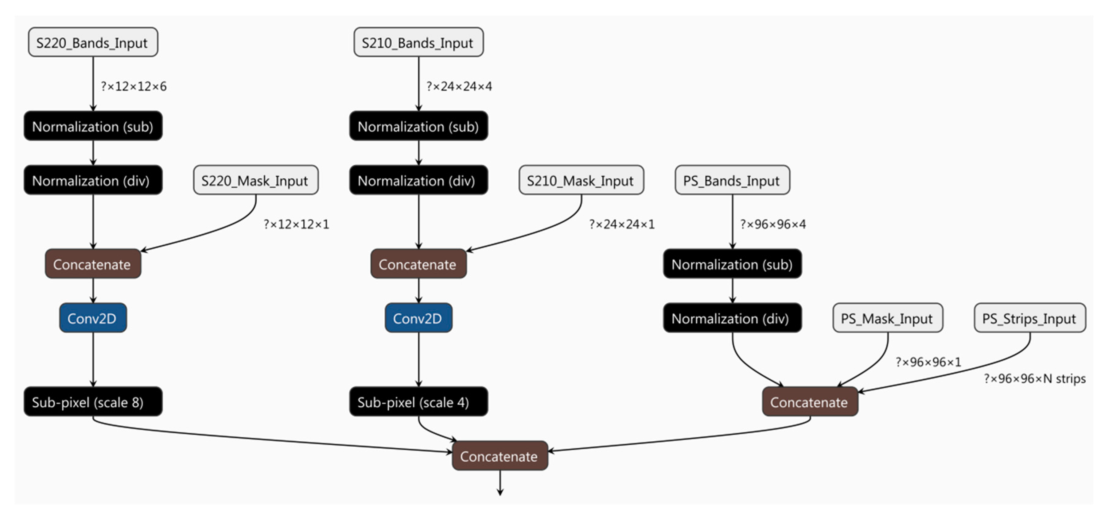
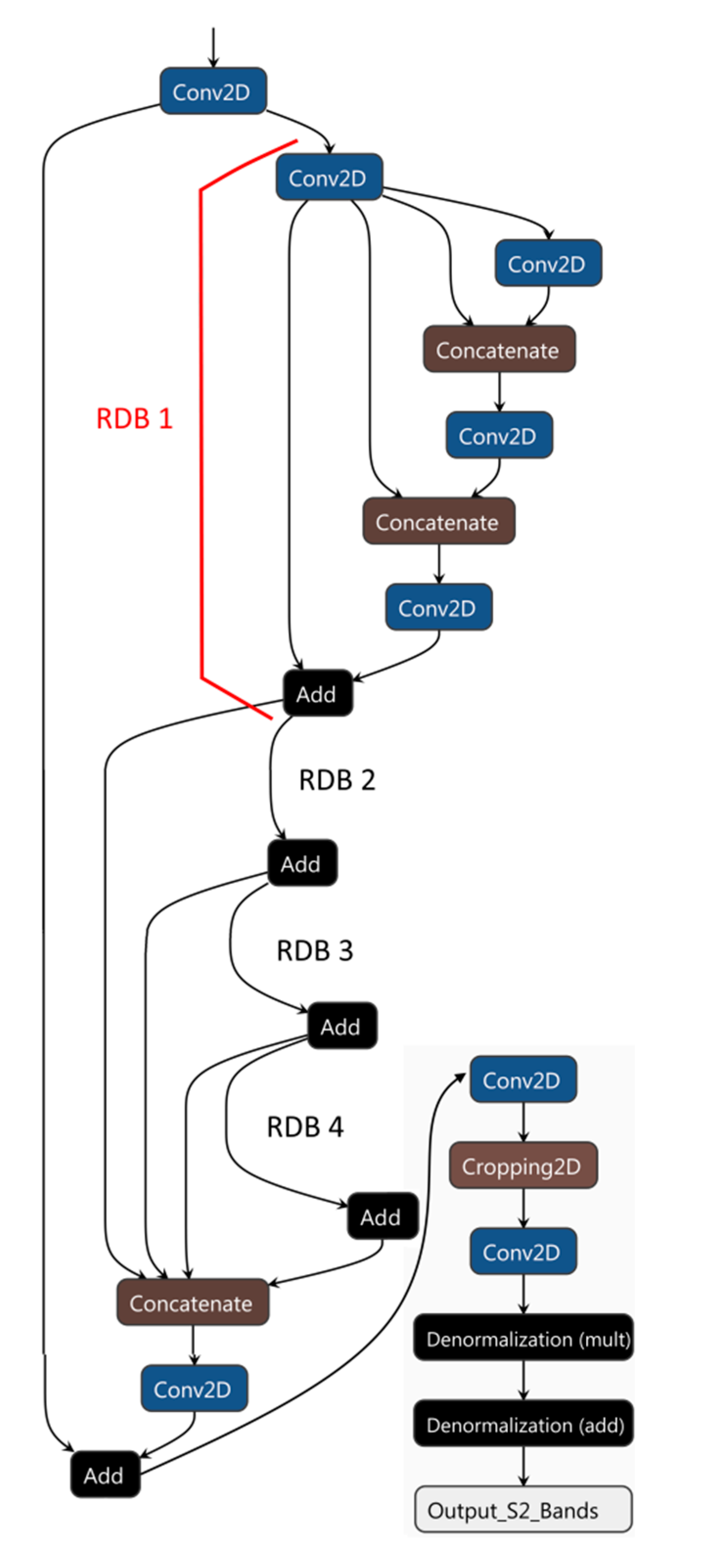
2.5. Network Architecture

As the relationships between variables in the spectral and spatial dimensions within and between S2 and PS images were a priori unknown, convolutional neural networks (CNNs) were used to directly learn from data. The proposed CNNs aimed at super-resolving the 10 bands of S2 to 2.5 m using intrinsic spectral-spatial information of PS. More particularly, CNNs with residual learning were implemented. For networks with numerous convolutions and layers, residual CNNs are known to be safer and easier to train [24,47], notably because they limit the problem of vanishing/exploding gradients [48,49].

For NN training, S2 ground truth at 2.5 m should ideally be used, but obviously did not exist. The Wald’s protocol was thus used [50]. It consists in using, as input, properly downsampled bands and, as output, the same bands but at the highest available resolution (

Table 2. Spatial resolution, patch size, and depth (number of channels) of input and output data for training and prediction of the two super-resolution neural networks (NNs): from 10 to 2.5 m (×4) and from 20 to 2.5 m (×8). PS, PlanetScope data; S210, Sentinel-2 10-m data; S220, Sentinel-2 20-m data. For resolutions, values not in brackets correspond to NN prediction. For patch sizes, values in brackets correspond to the overlapping pixels (both sides).

NN	Data	Source	Resolution (m)	Patch Size (px.)	Depth
×4	Input	PS	2.5 (10)	96 (16 + 16)	4 bands + 1 mask + number of strips
		S210	10 (40)	24 (4 + 4)	5 (4 bands + 1 mask)
		S220	20 (80)	12 (2 + 2)	7 (6 bands + 1 mask)
	Output	S210	2.5 (10)	64	4 bands
×8	Input	PS	2.5 (20)	96 (16 + 16)	4 bands + 1 mask + number of strips
		S210	10 (80)	24 (4 + 4)	5 (4 bands + 1 mask)
		S220	20 (160)	12 (2 + 2)	7 (6 bands + 1 mask)
	Output	S220	2.5 (20)	64	6 bands

). This protocol is based on the assumption that relationships between variables are scale invariant. Another solution could have been to use the method proposed by Galar et al. [29]. However, although avoiding data downsampling, bands of input and output would have to be equal in numbers and close in spectral ranges [24,29].

Two scale ratios (SRs) were applied: 4× (from 10 to 2.5 m) and 8× (from 20 to 2.5 m). Data at the desired SRs were generated by blurring with a Gaussian filter (standard deviation of 0.75 and 1.50 pixels, respectively) and then averaging over SR × SR windows [23]. The S2 10- and 20-m masks, and the PS mask and strips were downsampled using the “mode” resampling method (no blur).

The general network architecture was thought as the best compromise between super-resolution quality and performance efficiency. Several state-of-the-art residual-learning convolutional neural networks (RCNNs) for image super-resolution [47,48,49,51,52] were tested with some adaptations to include data of both constellations, Sentinel-2 (S2) and PlanetScope (PS), with different spatial resolutions and numbers of spectral bands (6 S2 bands at 20 m, 4 S2 bands at 10 m, and 4 PS bands at 2.5 m), as well as their corresponding masks of clouds and shadows. Although percentages of clouds and shadows were low in PS scenes (<5%), these additional data improved the local rendering of the super-resolved S2 images. PS strips were also included to normalize the pronounced radiometric inconsistencies between PS strips (Figure 3E,F).

Several configurations of super-resolution RCNNs were tested (patches size, number of filters, number of residual blocks, different loss functions, etc.) with encouraging results from the beginning. The main issue was to eliminate undesirable border effects of S2 output patches. These effects were smaller when using sub-pixel convolutions instead of transpose convolutions [53], before or after residual learning, but still undesirable. The border effects were further reduced using sub-pixel convolution followed by “mirror” padding [54] to increase patch size from 64 to 96 pixels (16 + 64 + 16). Small but visible differences were still present for a few pixels at the border of the output patches. The overall quality of super-resolution was not that much affected, but border effects were still disturbing for human eyes (when zooming). The proposed architecture resulted in the best radiometry normalization and super-resolution quality with no border effects.

Two RCNNs were implemented: one by scale ratio (4× and 8×). As the PS strips (and their number) varied between S2 tiles, RCNNs were trained from scratch for each S2 tile (no use of pre-trained NN or weights). The network architecture was the same for both RCNNs and was composed of three steps: data transformation (Figure 4), residual learning, and data reconstruction (Figure 5). S2 20-m (S220), S2 10-m (S210), and PS bands were normalized separately using Equation (1). Data normalization strongly enhances the performance and learning capacity of NNs and minimizes the error. PS mask, strips, and normalized bands were concatenated. S210 mask and normalized bands were concatenated. S220 mask and normalized bands were concatenated. S210 and S220 concatenations were upscaled using one sub-pixel convolution [51] of scale 4 (patch size from 24 to 96) and of scale 8 (patch size from 12 to 96), respectively (Table 2). Upscaled S210 and S220 data and PS data were concatenated and then used for residual learning. The residual learning was composed of four residual dense blocks (RDBs), and each RDB was composed of three convolutions and two concatenations. RDBs are described in detail in [52]. The padding was set to “same” (zero padding). The reconstruction consisted in one cropping to resize patches from 96 to 64 and eliminating the data affected by the zero padding (Table 2). A last convolution was applied to get the appropriate number of channels: 4 for the ×4 NN and 6 for the ×8 NN. Finally, the output data were denormalized (i.e., reverse of Equation (1)).

$$NormVa{l}_b=(Va{l}_b-P_{1s{t}_b})\times \left(P_{99t{h}_b}-P_{1s{t}_b}\right)$$

(1)

where $Va{l}_b$ denotes the spectral values of the considered band $b$, $P_{1s{t}_b}$ and $P_{99t{h}_b}$ denote the first and 99th percentiles of the values of band $b$, and $NormVa{l}_b$ denotes the normalized values of the band $b$.

For all convolutions in RDBs, the kernel size was 3 × 3 and the activation function was rectified linear unit (ReLU). The number of filters was 128 between RDBs and 64 inside RDBs [52]. For data transformation and reconstruction, kernel size was 1 × 1 and the activation function was linear. The total number of parameters, varying between S2 tiles and NNs, was about 2,550,000.

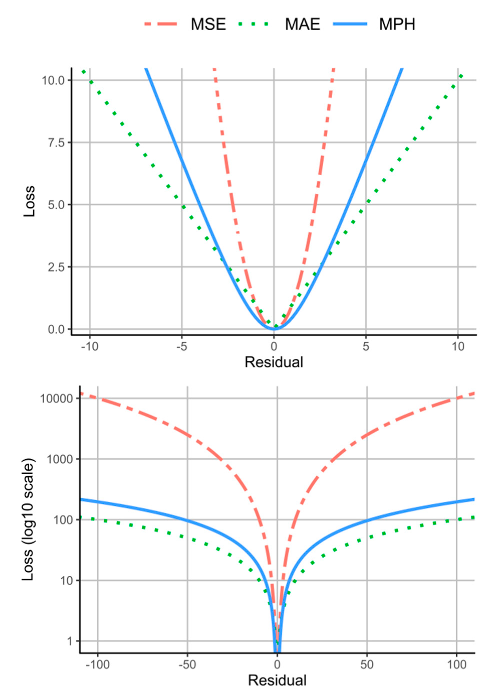
2.6. Network Training

The configuration was the same for both NNs. For each NN, 3000 batches were used as training data. The batch size was 32 samples, one sample corresponding to a whole set of PS, S210, and S220 patches (Table 2). For each batch, the 32 samples were randomly extracted. The Adam optimizer [55] was used with a learning rate of 1e⁻⁴ and a decay of 5e⁻⁵. The number of epochs was 100 and the number of steps per epoch was 300. For each NN, the parameters where thus updated 960,000 times (=100 × 300 × 32). When the training stopped, the loss value was at the beginning of the learning plateau [56]. A higher number epoch, such as 150 or 200, could have slightly increased the quality but at a cost of a too long processing time and with an increasing risk of overfitting.

Concerning loss function, performance and results using the mean absolute error (MAE or “l1”) or the mean squared error (MSE or “l2”) were not satisfying. MSE is easier to solve but MAE is more robust to outliers. While MSE is the dominant NN measure, it was shown that MAE performed better than MSE for single image super-resolution [57]. Considering the lower quality of radiometry between and within PS scenes, using MSE with a non-negligible proportion of outliers was problematic. On the other hand, the training time was longer using MAE and resulted in a lesser overall quality. As an intermediate solution, the mean pseudo-Huber (MPH) [58] was used (Equation (2) with a delta value of 2). MPH behaves as MSE near the origin (low residuals) and as MAE elsewhere (Figure 6). Furthermore, as the value range varied significantly between the 10 S2 bands, the residuals were weighted using Equation (3) before MPH computation.

$$PH={\delta }^2\times \left(\sqrt{1+{\left(\frac{RS}{\delta }\right)}^2}-1\right)$$

(2)

where $\delta$ denotes the delta value and $RS$ denotes the residuals (i.e., ground truth minus prediction).

$$WeightR{S}_b=R{S}_b÷ (P_{99t{h}_b}-P_{1s{t}_b})\times MeanRng$$

(3)

where $R{S}_b$ denotes the residuals for the considered band $b$, $P_{1s{t}_b}$ and $P_{99t{h}_b}$ denote the first and 99th percentiles of the values of band $b$, $MeanRng$ denotes the mean of the value ranges of all bands (6 for S220 and 4 for S210), and $WeightR{S}_b$ denotes the weighted residuals of band $b$ injected in Equation (2) for computing MPH (Equation (2)).

2.7. Quality Assessment

The radiometric normalization and super-resolution quality were assessed at ground truth resolution for the two NNs (10 m for ×4 NN and 20 m for ×8 NN) considering the whole S2 tile (not only the training data) and using seven measures [59,60]: mean error (ME), mean absolute error (MAE), mean weighted absolute error (MWAE), root mean square error (RMSE), peak signal noise ratio (PSNR), structure similarity (SSIM), and cross correlation (CC). MWAE is similar to MAE but computed from absolute residuals divided by the band value range ($P_{99t{h}_b}-{ \mathrm{P}}_{1s{t}_b}$) and expressed in percentage. SSIM and PSNR are the most commonly considered metrics for image super-resolution [61]. SSIM measures the similarity between the signals of ground truth and predicted images. PSNR is the ratio between the maximum possible power of the signal and the power of corrupting noise. SSIM and PSNR were computed with a max value of 2¹⁶. ME values close to zero; lower values of MAE, MWAE, and RMSE; and higher values of the PSNR, SSIM and CC indicate better quality. In addition, the quality was also assessed visually (photointerpretation), with attention given to the borders of output patches and to areas with variation in PS radiometry (different strips) and presence of clouds and shadows.

3. Results

3.1. Measured Quality

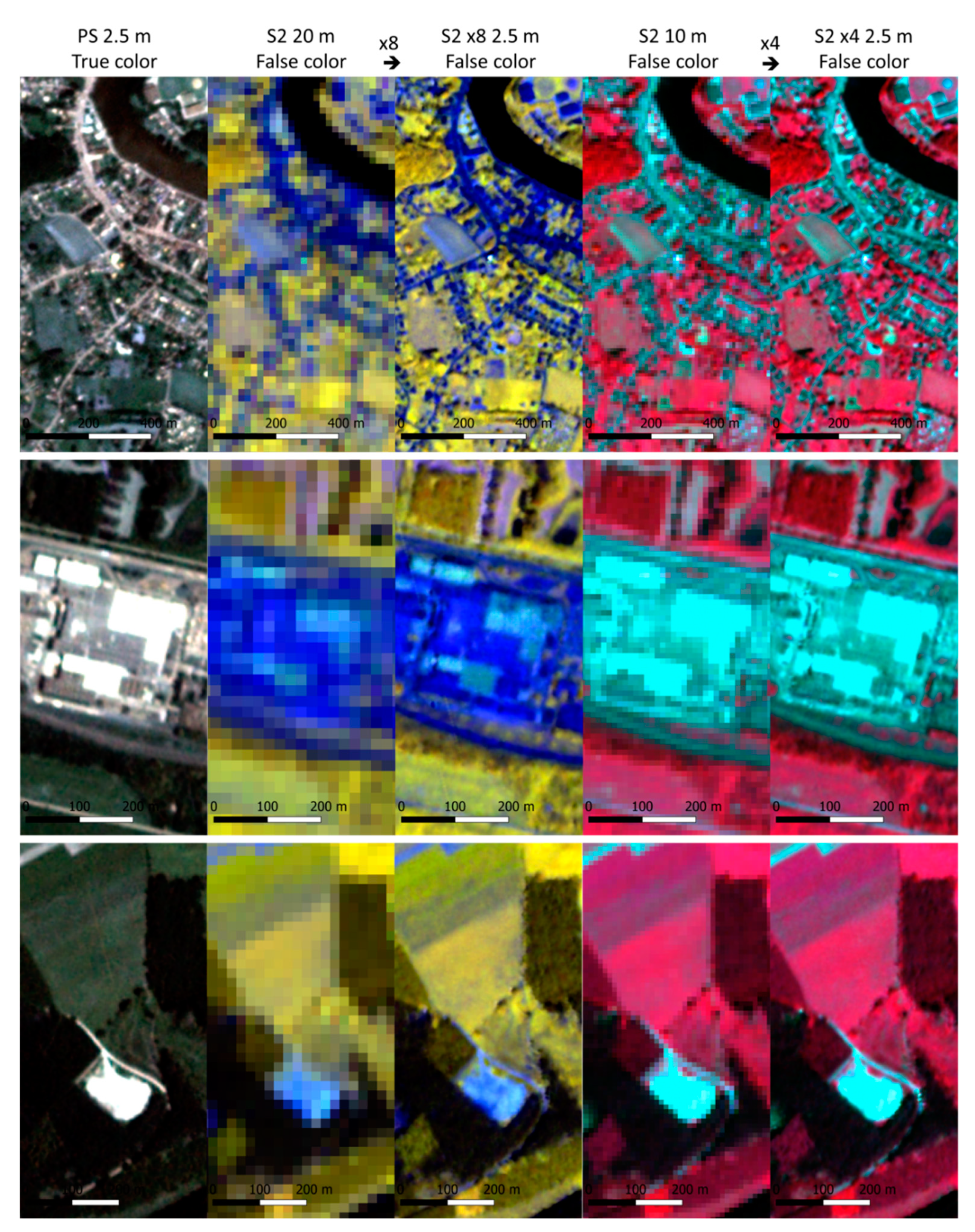
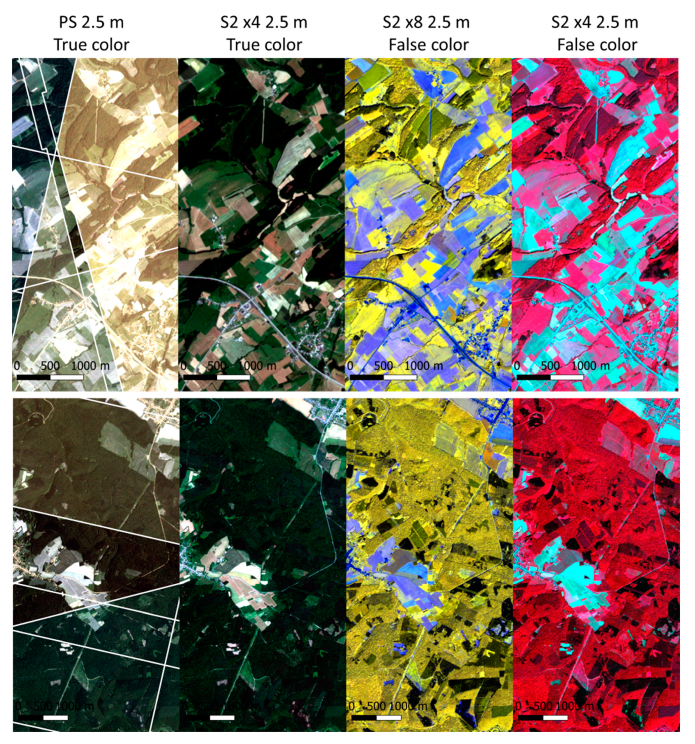
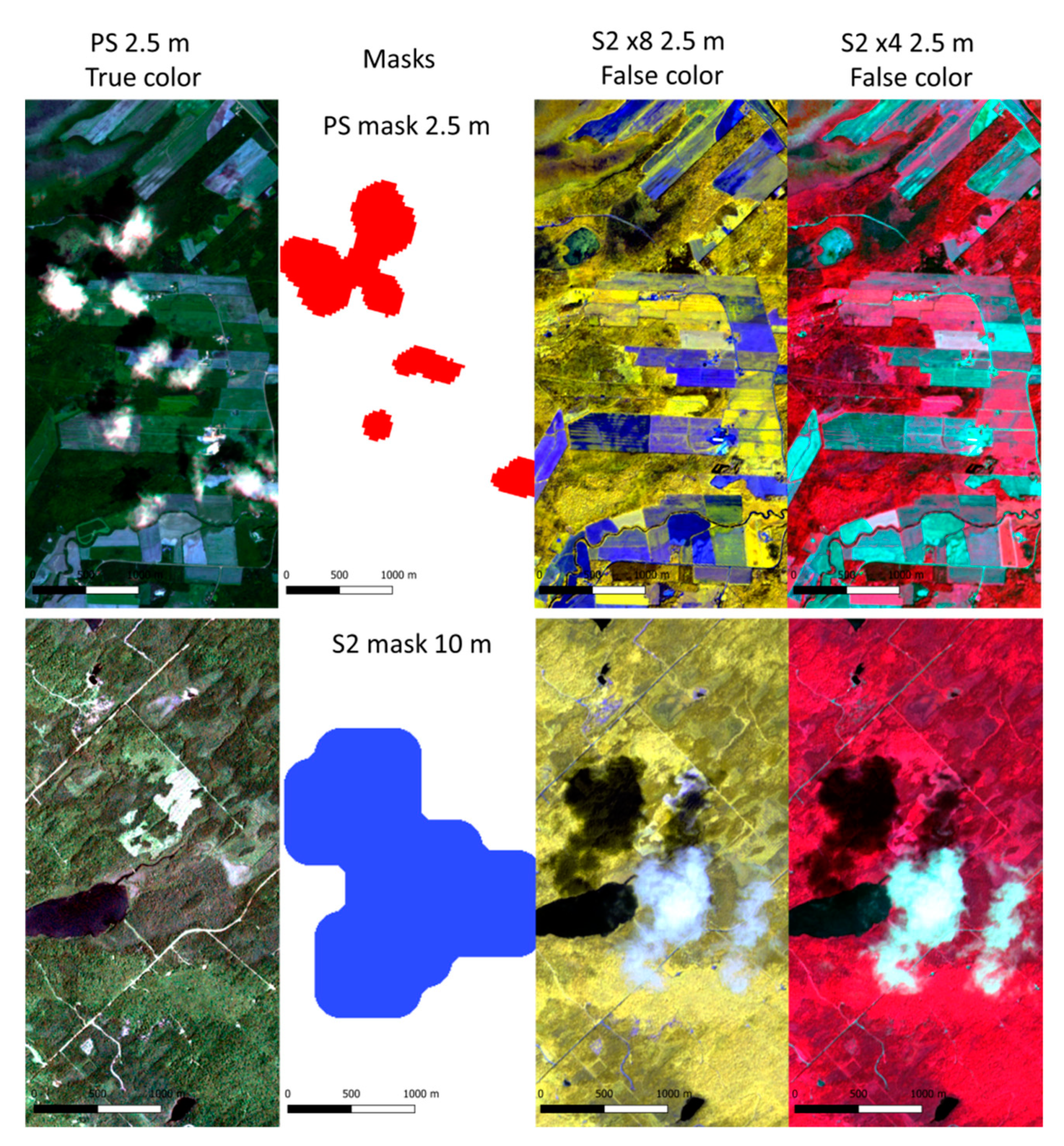
The radiometric normalization and super-resolution quality was assessed by NN (at 10 m for ×4 and 20 m for ×8) for the six S2 tiles: whole tile and all bands together (

Table 3. Measured quality of the two super-resolution neural networks (NNs): from 10 to 2.5 m (×4) and from 20 to 2.5 m (×8). Overall quality (i.e., whole tile and all bands together) for the six selected S2 tiles (Figure 2) (Table 1). ME, mean error; MAE, mean absolute error; MWAE (%), mean weighted absolute error; RMSE, root mean square error; PSNR, peak signal noise ratio; SSIM, structure similarity. CC, cross correlation.

NN	S2 Tile	ME	MAE	MWAE	RMSE	PSNR	SSIM	CC
×4 (10 m)	BeS	2.5	36.2	2.3	69.0	59.6	1.000	0.999
	BeN	−2.8	43.9	2.0	83.3	57.9	1.000	0.998
	Bra	0.1	25.0	1.5	41.7	63.9	1.000	0.999
	Can	−5.1	41.0	2.9	80.6	58.2	1.000	0.998
	Chi	−1.5	40.0	2.4	71.4	59.3	1.000	0.998
	Mad	1.5	37.0	1.6	54.4	61.6	1.000	0.998
×8 (20 m)	BeS	−5.9	67.8	2.4	100.7	56.3	1.000	0.997
	BeN	5.6	76.5	2.0	121.2	54.7	1.000	0.995
	Bra	5.5	52.8	1.5	79.2	58.3	1.000	0.996
	Can	14.4	67.9	2.3	101.8	56.2	1.000	0.997
	Chi	1.0	68.4	2.2	99.8	56.4	1.000	0.994
	Mad	8.6	66.0	2.1	95.7	56.7	1.000	0.994

) and with a focus on PS strips (

Table 4. Measured quality of the two super-resolution neural networks (NNs): from 10 to 2.5 m (×4) and from 20 to 2.5 m (×8). Focus on variations between PS strips for the six selected S2 tiles. ME, mean error; MAE, mean absolute error; RMSE, root mean square error; CC, cross correlation. The values correspond to mean (standard deviation) of the quality measures computed separately for each PS strip. See Table 1 for the number of strips by tile.

NN	S2 Tile	ME	MAE	RMSE	CC
×4 (10 m)	BeS	1.5 (14)	44.9 (17.4)	79.5 (27.5)	0.998 (0.001)
	BeN	−2.7 (3.9)	43.5 (11.9)	78.8 (24.4)	0.995 (0.006)
	Bra	1.2 (6.3)	30.3 (10.2)	48.6 (14.7)	0.999 (0.001)
	Can	−6.3 (5.4)	41.8 (10.8)	80.2 (20.5)	0.998 (0.001)
	Chi	−1.0 (3.0)	46.0 (15.6)	80.5 (26.3)	0.997 (0.003)
	Mad	0.9 (4.3)	37.1 (7.2)	53.3 (10.1)	0.998 (0.001)
×8 (20 m)	BeS	−1.8 (20.0)	77.6 (19.9)	113.2 (26.0)	0.996 (0.002)
	BeN	4.9 (6.4)	72.3 (25.0)	114.2 (38.7)	0.991 (0.010)
	Bra	8.3 (14.1)	59.6 (10.6)	86.9 (13.6)	0.995 (0.002)
	Can	12.4 (7.4)	70.3 (16.1)	110.8 (52.3)	0.996 (0.005)
	Chi	3.3 (7.2)	78.1 (18.7)	113.5 (26.8)	0.992 (0.005)
	Mad	8.1 (3.9)	66.9 (7.6)	96.8 (9.4)	0.993 (0.002)

). The quality was also assessed by band (

Table 5. Measured quality of the two super-resolution neural networks (NNs), from 10 to 2.5 m (×4) and from 20 to 2.5 m (×8), by band (10 bands) for the two Belgian S2 tiles (BeS and BeN) (Figure 3). ME, mean error; MAE, mean absolute error; MWAE (%), mean weighted absolute error. RMSE, root mean square error; PSNR, peak signal noise ratio; SSIM, structure similarity; CC, cross correlation; PRg, 1st‒99th percentiles of ground truth data; PRp, 1st‒99th percentiles of predicted data.

S2 Tile	NN	Band	ME	MAE	MWAE	RMSE	PSNR	SSIM	CC	PRg	PRp
BeS	×4 (10 m)	B2	1.2	16.1	1.0	31.6	66.3	1.000	0.991	2‒1049	8‒1042
		B3	2.1	20.9	1.3	35.5	65.3	1.000	0.993	160‒1492	164‒1482
		B4	10.2	23.5	1.5	41.7	63.9	0.999	0.995	25‒1830	21‒1805
		B8	−3.6	84.4	5.3	122.7	54.6	0.997	0.991	1315‒5514	1339‒5506
	×8 (20 m)	B5	−6.3	35.4	1.2	54.2	61.7	0.999	0.992	339‒2211	350–2200
		B6	−4.8	70.2	2.5	97.9	56.5	0.998	0.988	1150‒4142	1159‒4138
		B7	−5.7	81.2	2.9	114	55.2	0.997	0.99	1376‒5310	1399‒5304
		B8A	−6.8	84	3.0	118.1	54.9	0.997	0.991	1533‒5694	1559‒5693
		B11	−5.4	82.1	2.9	117.9	54.9	0.997	0.985	681‒3848	689‒3837
		B12	−6.7	53.8	1.9	86.5	57.6	0.998	0.986	274‒2609	283‒2607
BeN	×4 (10 m)	B2	−3.7	27.2	1.2	58.7	61.0	0.999	0.986	0‒1594	10‒1593
		B3	2.4	30	1.3	59.8	60.8	0.999	0.987	172‒1961	175‒1948
		B4	3.7	34.4	1.5	67.2	59.8	0.999	0.993	0‒2339	0‒2327
		B8	−13.6	83.8	3.7	127.4	54.2	0.997	0.996	22‒5956	40‒5942
	×8 (20 m)	B5	1.6	46.6	1.2	80.3	58.2	0.999	0.985	154‒2487	161‒2459
		B6	2.7	75.4	2.0	114.8	55.1	0.997	0.993	48‒4304	55‒4273
		B7	6.4	86.4	2.3	130.2	54.0	0.997	0.995	43‒5796	51‒5748
		B8A	7.4	87.4	2.3	131.9	53.9	0.997	0.996	12‒6092	24‒6065
		B11	4.2	85.7	2.3	130.9	54.0	0.996	0.985	5‒3634	11‒3596
		B12	11.5	77.6	2.0	130.6	54.0	0.996	0.986	16‒3340	18‒3291

) and by main land cover (

Table 6. Measured quality of the two super-resolution neural networks (NNs), from 10 to 2.5 m (×4) and from 20 to 2.5 m (×8), by main land cover (Corine Land Cover 2018) of the two Belgian S2 tiles (BeS and BeN together) (Figure 3). ME, mean error; MAE, mean absolute error; RMSE, root mean square error; CC, cross correlation.

NN	CLC Category (Level 1)	Area (%)	ME	MAE	RMSE	CC
×4 (10 m)	Artificial surfaces	18.0	0.0	60.2	109.1	0.995
	Agricultural areas	54.2	−1.0	35.9	66.5	0.999
	Forest and seminatural areas	23.9	1.6	36.8	71.3	0.999
	Wetlands	0.6	−3.4	38.6	76.7	0.995
	Water bodies	3.3	0.2	22.8	43.8	0.994
×8 (20 m)	Artificial surfaces	18.0	4.5	97.0	152.8	0.987
	Agricultural areas	54.2	−0.6	70.9	105.7	0.996
	Forest and seminatural areas	23.9	−2.5	63.3	91.6	0.997
	Wetlands	0.6	−2.6	60.3	97.5	0.995
	Water bodies	3.3	−1.1	24.4	54.0	0.994

) for the two Belgian tiles (“BeS” and “BeN”).

The overall quality of the six tiles was very good (Table 3) with low values in MAE, MWAE, RMSE, and MPH; high values in PNSR, SSIM, and CC; and ME values close to zero (no bias). SSIM values computed from the four predicted bands for ×4 NN and the six predicted bands for ×8 NN reached the maximum value of 1 (by rounding), indicating that the two images are (almost) perfectly structurally similar [57]. PSNR and SSIM values were systematically higher than those of Galar et al. [29], a unique and most similar study, but using a different approach. Their highest PSNR and SSIM values were 35.5 and 0.957, respectively. The MWAE, expressing the error in percentage of the band value ranges, varied from 1.5% to 2.9%. The quality variations between PS strips were low (Table 4), confirming that the method accurately captured and corrected the PS radiometric inconsistencies at the scale of the S2 tile.

The quality of each of the 10 predicted bands was high with no major differences (Table 5). The MWAE varied from 1% to 5.3%. Although the bands B5, B6, B11, and B12 presented no overlapping with the PS bands (Figure 1), their error was close to the average. Surprisingly, the band B8 was the less well predicted of all bands. Concerning the quality by land cover (Table 6), no major differences were highlighted but artificial surfaces were logically less well predicted than less spectrally and spatially contrasted areas such as agricultural and forest lands.

3.2. Visual Quality

The proposed method was also validated by photointerpretation (Figure 7). There was no border effect even at maximum zoom. The output patches were thus not distinguishable from each other at coarser and finer resolutions. The normalization of the radiometric inconsistencies between PS strips was impressive (Figure 8). In the super-resolved images (10 S2 bands at 2.5 m), no differences were observed. A 1-pixel between-scenes boundary was sometime visible (but with very similar spectral values). This boundary was probably indirectly induced by the training data downsampling (resampling of the PS strips mosaic using the “mode” method). The effect of clouds and shadows in PS scenes on super-revolved images was limited as they simply did not appear (Figure 9, Top). However, these areas were slightly affected by speckle and/or blur, decreasing locally the visual quality. For clouds and shadows in S2 tiles, they were fully predicted (Figure 9, Bottom).

3.3. Processing Times

The processing times using a unique computer and for a given S2 tile were on average: about 1 h 30 min for the selection, downloading, and preparation of images; about 2 × 4 h for the preparation of the 2 × 3000 training batches; about 2 × 8 h for the NN trainings; about 1 h 15 min for the prediction at the coarser resolution (four bands at 10 m and six bands at 20 m); and about 21 h for the prediction at finer resolution (10 bands at 2.5 m). The total time for the complete procedure was thus about 48 h.

4. Discussion

In this study, we presented and validated a novel method for super-resolving Sentinel-2 (S2) imagery (10 bands from 10 or 20 to 2.5 m). Super-resolution was achieved by fusion with additional images acquired at finer resolution by the PlanetScope (PS) constellation. The super-resolution quality was thoroughly analyzed for six S2 tiles acquired in contrasted conditions over five countries around the world, confirming that the proposed method is highly accurate and robust. The method also remarkably normalized the radiometric inconsistencies between PS micro-satellites. Super-resolution and radiometric normalization were achieved simultaneously using state-of-the-art residual convolutional neural networks (RCNNs), adapted to the particularities of S2 and PS imageries, and including the corresponding masks of clouds and shadows.

To our knowledge, only one study [29] considered a similar approach combining S2 and RapidEye images for super-resolving three of the S2 bands (B2, B3, and B4) to 5 m, also using RCNNs, but with an architecture originally developed for conventional “RGB” images. With a spatial resolution of 2.5 m, the generalization of the procedure to 10 S2 bands (B2, B3, B4, B8, B5, B6, B7, B8a, B11, and B12) and a much higher accuracy, this study further explored the high potential of deep learning for multi-satellite multi-sensor image fusion. The proposed method is highly spatially and spectrally accurate, at the scale of the considered S2 tile, but also locally, and separately for each band, PS strip (i.e., unique PS satellite and orbit), and main land cover.

Radiometric inconsistencies between PS strips are mainly related to differences in sensor spectral response, orbital configuration [31,32], and acquisition date/time. The proposed method accurately captures and corrects these radiometric variations. As the PS strips varied for each S2 tile, the RCNNs had to be train from scratch every time (no use of pre-trained NN or weights). Although it strongly increases robustness, the processing time could be limiting for routine use. With a unique computer, 48 h per S2 tile were necessary. This processing time could be significantly decreased with code optimization and implementation in powerful cloud computing platforms, such as Google Earth Engine.

The high temporal resolution of PS imagery (revisit time of one day) is an important element. The small acquisition time differences between the S2 tile and PS scenes strongly limit land cover changes. Contrary to Shao et al. [15], fusing Landsat-8 and S2 imageries, the use of temporal series was not necessary.

We deliberately selected S2 tiles and PS scenes with low percentages of clouds and shadows (<5%). The inclusion of S2 and PS masks in the network architecture improved the local rendering of the super-resolved images. Clouds and shadows in S2 were fully predicted. Clouds and shadows in PS scenes were not predicted but with speckle and/or blur effects. The proposed method should be tested with higher percentages of clouds and shadows. RCNNs should be able to learn and adapt the prediction. However, for percentages > 20%, it would probably be more appropriate to use only data free of clouds and shadows. The super-resolution quality would be identical but with a higher proportion of missing data.

The proposed method could also be applied to images of other satellite constellations. For instance, S2 could be replaced by Landsat and PS by Pleiades. However, it would be important to keep in mind that the proposed method is based on the scale-invariant hypothesis [50]. We demonstrated that the ×8 scale ratio (from 20 to 2.5 m) resulted in high quality super-resolution, but the quality for the 4× scale ratio (from 10 to 2.5 m) was as expected higher. The maximum scale ratio is still to be determined.

The proposed RCNN architecture could probably still be improved in several ways. Data augmentation is a well-known way to improve the performance of deep networks. For image super-resolution, some of the augmentation methods highlighted by Ghaffar et al. [62] could be added. The “CutBlur” approach could also be tested [63], as well as the use of the FReLU activation function [64], instead of ReLU, for residual learning. Residual learning could be done first, separately for S220, S210, and PS data (three branches, similarly to Wu et al. [28]) and then together (single branch). Concerning loss functions, as the pseudo-Huber resulted in better predictions and performance than with the usual MAE and MSE, the robust adaptive loss function [58] looks promising.

5. Conclusions

The proposed method allows super-resolving 10 bands of the Sentinel-2 imagery, from 20 or 10 to 2.5 m, at a very high spatial and spectral accuracy. The method is robust and can be applied to S2 tiles acquired worldwide at any date.

References

1. Unninayar, S.; Olsen, L.M. Monitoring, observations, and remote sensing—Global dimensions. In Reference Module in Earth Systems and Environmental Sciences; Elsevier: Amsterdam, The Netherlands, 2015; ISBN 978-0-12-409548-9. [Google Scholar]
2. Vivone, G.; Alparone, L.; Chanussot, J.; Mura, M.D.; Garzelli, A.; Licciardi, G.A.; Restaino, R.; Wald, L. A critical comparison among pansharpening algorithms. IEEE Trans. Geosci. Remote Sens. 2015, 53, 2565–2586. [Google Scholar] [CrossRef]
3. Garzelli, A. A review of image fusion algorithms based on the super-resolution paradigm. Remote Sens. 2016, 8, 797. [Google Scholar] [CrossRef] [Green Version]
4. Pohl, C.; Van Genderen, J.L. Review article Multisensor image fusion in remote sensing: Concepts, methods and applications. Int. J. Remote Sens. 1998, 19, 823–854. [Google Scholar] [CrossRef] [Green Version]
5. Ghassemian, H. A review of remote sensing image fusion methods. Inf. Fusion 2016, 32, 75–89. [Google Scholar] [CrossRef]
6. Meng, X.; Shen, H.; Li, H.; Zhang, L.; Fu, R. Review of the pansharpening methods for remote sensing images based on the idea of meta-analysis: Practical discussion and challenges. Inf. Fusion 2019, 46, 102–113. [Google Scholar] [CrossRef]
7. Li, S.; Kang, X.; Fang, L.; Hu, J.; Yin, H. Pixel-Level image fusion: A survey of the state of the art. Inf. Fusion 2017, 33, 100–112. [Google Scholar] [CrossRef]
8. Ma, L.; Liu, Y.; Zhang, X.; Ye, Y.; Yin, G.; Johnson, B.A. Deep learning in remote sensing applications: A meta-analysis and review. ISPRS J. Photogramm. Remote Sens. 2019, 152, 166–177. [Google Scholar] [CrossRef]
9. Shao, Z.; Cai, J. Remote sensing image fusion with deep convolutional neural network. IEEE J. Sel. Top. Appl. Earth Obs. Remote Sens. 2018, 11, 1656–1669. [Google Scholar] [CrossRef]
10. Wei, Y.; Yuan, Q.; Shen, H.; Zhang, L. Boosting the accuracy of multispectral image pansharpening by learning a deep residual network. IEEE Geosci. Remote Sens. Lett. 2017, 14, 1795–1799. [Google Scholar] [CrossRef] [Green Version]
11. Gargiulo, M.; Mazza, A.; Gaetano, R.; Ruello, G.; Scarpa, G. A CNN-Based fusion method for super-resolution of Sentinel-2 data. In Proceedings of the IGARSS 2018-2018 IEEE International Geoscience and Remote Sensing Symposium, Valencia, Spain, 22–27 July 2018; pp. 4713–4716. [Google Scholar]
12. Hu, J.; He, Z.; Wu, J. Deep self-learning network for adaptive pansharpening. Remote Sens. 2019, 11, 2395. [Google Scholar] [CrossRef] [Green Version]
13. Pohl, C. Multisensor image fusion guidelines in remote sensing. In Proceedings of the 9th Symposium of the International Society for Digital Earth (ISDE), Halifax, Canada, 5–9 October 2015; Volume 34, p. 012026. [Google Scholar]
14. Park, S.C.; Park, M.K.; Kang, M.G. Super-Resolution image reconstruction: A technical overview. IEEE Signal Process. Mag. 2003, 20, 21–36. [Google Scholar] [CrossRef] [Green Version]
15. Shao, Z.; Cai, J.; Fu, P.; Hu, L.; Liu, T. Deep learning-based fusion of Landsat-8 and Sentinel-2 images for a harmonized surface reflectance product. Remote Sens. Environ. 2019, 235, 111425. [Google Scholar] [CrossRef]
16. Feng, G.; Masek, J.; Schwaller, M.; Hall, F. On the blending of the Landsat and MODIS surface reflectance: Predicting daily Landsat surface reflectance. IEEE Trans. Geosci. Remote Sens. 2006, 44, 2207–2218. [Google Scholar] [CrossRef]
17. Zhu, X.; Chen, J.; Gao, F.; Chen, X.; Masek, J.G. An enhanced spatial and temporal adaptive reflectance fusion model for complex heterogeneous regions. Remote Sens. Environ. 2010, 114, 2610–2623. [Google Scholar] [CrossRef]
18. Wang, Q.; Blackburn, G.A.; Onojeghuo, A.O.; Dash, J.; Zhou, L.; Zhang, Y.; Atkinson, P.M. Fusion of Landsat 8 OLI and Sentinel-2 MSI Data. IEEE Trans. Geosci. Remote Sens. 2017, 55, 3885–3899. [Google Scholar] [CrossRef] [Green Version]
19. Benediktsson, J.A.; Chanussot, J.; Moon, W.M. Very high-resolution remote sensing: Challenges and opportunities [Point of View]. Proc. IEEE 2012, 100, 1907–1910. [Google Scholar] [CrossRef]
20. Benediktsson, J.; Chanussot, J.; Moon, W. Advances in very-high-resolution remote sensing. Proc. IEEE 2013, 101, 566–569. [Google Scholar] [CrossRef]
21. Liebel, L.; Körner, M. Single-Image super resolution for multispectral remote sensing data using convolutional neural networks. ISPRS Int. Arch. Photogramm. Remote Sens. Spat. Inf. Sci. 2016, 41B3, 883–890. [Google Scholar] [CrossRef]
22. Lanaras, C.; Bioucas-Dias, J.; Baltsavias, E.; Schindler, K. Super-Resolution of multispectral multiresolution images from a single sensor. In Proceedings of the 2017 IEEE Conference on Computer Vision and Pattern Recognition Workshops (CVPRW), Honolulu, HI, USA, 21–26 July 2017; pp. 1505–1513. [Google Scholar]
23. Lanaras, C.; Bioucas-Dias, J.; Galliani, S.; Baltsavias, E.; Schindler, K. Super-Resolution of Sentinel-2 images: Learning a globally applicable deep neural network. ISPRS J. Photogramm. Remote Sens. 2018, 146, 305–319. [Google Scholar] [CrossRef] [Green Version]
24. Palsson, F.; Sveinsson, R.J.; Ulfarsson, O.M. Sentinel-2 Image fusion using a deep residual network. Remote Sens. 2018, 10, 1290. [Google Scholar] [CrossRef] [Green Version]
25. Gargiulo, M.; Mazza, A.; Gaetano, R.; Ruello, G.; Scarpa, G. Fast super-resolution of 20 m Sentinel-2 bands using convolutional neural networks. Remote Sens. 2019, 11, 2635. [Google Scholar] [CrossRef] [Green Version]
26. Wang, J.; Huang, B.; Zhang, H.K.; Ma, P. Sentinel-2A image fusion using a machine learning approach. IEEE Trans. Geosci. Remote Sens. 2019, 57, 9589–9601. [Google Scholar] [CrossRef]
27. Ulfarsson, M.O.; Palsson, F.; Mura, M.D.; Sveinsson, J.R. Sentinel-2 sharpening using a reduced-rank method. IEEE Trans. Geosci. Remote Sens. 2019, 57, 6408–6420. [Google Scholar] [CrossRef]
28. Wu, J.; He, Z.; Hu, J. Sentinel-2 Sharpening via parallel residual network. Remote Sens. 2020, 12, 297. [Google Scholar] [CrossRef] [Green Version]
29. Galar, M.; Sesma, R.; Ayala, C.; Aranda, C. Super-Resolution for sentinel-2 images. ISPRS Int. Arch. Photogramm. Remote Sens. Spat. Inf. Sci. 2019, XLII-2/W16, 95–102. [Google Scholar] [CrossRef] [Green Version]
30. He, J.; Li, J.; Yuan, Q.; Li, H.; Shen, H. Spatial–Spectral fusion in different swath widths by a recurrent expanding residual convolutional neural network. Remote Sens. 2019, 11, 2203. [Google Scholar] [CrossRef] [Green Version]
31. Leach, N.; Coops, N.C.; Obrknezev, N. Normalization method for multi-sensor high spatial and temporal resolution satellite imagery with radiometric inconsistencies. Comput. Electron. Agric. 2019, 164, 104893. [Google Scholar] [CrossRef]
32. Houborg, R.; McCabe, F.M. Daily retrieval of NDVI and LAI at 3 m resolution via the fusion of cubesat, landsat, and MODIS data. Remote Sens. 2018, 10, 890. [Google Scholar] [CrossRef] [Green Version]
33. Houborg, R.; McCabe, M.F. A cubesat enabled Spatio-temporal enhancement method (CESTEM) utilizing planet, landsat and MODIS data. Remote Sens. Environ. 2018, 209, 211–226. [Google Scholar] [CrossRef]
34. R core team. R: A Language and Environment for Statistical Computing; R Foundation for Statistical Computing: Vienna, Austria, 2019; Available online: http://www.R-project.org/ (accessed on 1 May 2020).
35. Hijmans, R.J. Raster: Geographic Data Analysis and Modeling. 2019. Available online: https://cran.r-project.org/web/packages/raster/raster.pdf (accessed on 1 May 2020).
36. Pebesma, E. Simple features for R: Standardized support for spatial vector data. R J. 2018, 10, 439–446. [Google Scholar] [CrossRef] [Green Version]
37. Allaire, J.J.; Chollet, F. Keras: R Interface to “Keras”. 2019. Available online: https://keras.rstudio.com/ (accessed on 1 May 2020).
38. GDAL/OGR Contributors. GDAL/OGR Geospatial Data Abstraction Software Library; Open Source Geospatial Foundation: Beaverton, OR, USA, 2020. [Google Scholar]
39. Inglada, J.; Christophe, E. The Orfeo Toolbox remote sensing image processing software. In Proceedings of the 2009 IEEE International Geoscience and Remote Sensing Symposium, Cape Town, South Africa, 12–17 July 2009; Volume 4, p. IV-733. [Google Scholar]
40. Grizonnet, M.; Michel, J.; Poughon, V.; Inglada, J.; Savinaud, M.; Cresson, R. Orfeo ToolBox: Open source processing of remote sensing images. Open Geospatial Data Softw. Stand. 2017, 2, 15. [Google Scholar] [CrossRef] [Green Version]
41. Laviron, X. theiaR: Download and Manage Data from Theia. 2020. Available online: https://cran.r-project.org/web/packages/theiaR/theiaR.pdf (accessed on 1 May 2020).
42. Lonjou, V.; Desjardins, C.; Hagolle, O.; Petrucci, B.; Tremas, T.; Dejus, M.; Makarau, A.; Auer, S. MACCS-ATCOR Joint Algorithm (MAJA). In Remote Sensing of Clouds and the Atmosphere XXI; International Society for Optics and Photonics: Bellingham, WA, USA, 2016. [Google Scholar]
43. Baetens, L.; Desjardins, C.; Hagolle, O. Validation of copernicus sentinel-2 cloud masks obtained from MAJA, Sen2Cor, and FMask Processors Using reference cloud masks generated with a supervised active learning procedure. Remote Sens. 2019, 11, 433. [Google Scholar] [CrossRef] [Green Version]
44. Sanchez, H.A.; Picoli, C.A.M.; Camara, G.; Andrade, R.P.; Chaves, E.D.M.; Lechler, S.; Soares, R.A.; Marujo, F.B.R.; Simões, E.O.R.; Ferreira, R.K.; et al. Comparison of Cloud cover detection algorithms on sentinel–2 images of the amazon tropical forest. Remote Sens. 2020, 12, 1284. [Google Scholar] [CrossRef] [Green Version]
45. Leutner, B.; Horning, N.; Schwalb-Willmann, J. RStoolbox: Tools for Remote Sensing Data Analysis. 2019. Available online: https://cran.r-project.org/web/packages/RStoolbox/RStoolbox.pdf (accessed on 1 May 2020).
46. Scheffler, D.; Hollstein, A.; Diedrich, H.; Segl, K.; Hostert, P. AROSICS: An automated and robust open-source image co-registration software for multi-sensor satellite data. Remote Sens. 2017, 9, 676. [Google Scholar] [CrossRef] [Green Version]
47. He, K.; Zhang, X.; Ren, S.; Sun, J. Deep residual learning for image recognition. In Proceedings of the 2016 IEEE Conference on Computer Vision and Pattern Recognition (CVPR), Las Vegas, NV, USA, 27–30 June 2016; pp. 770–778. [Google Scholar]
48. Lim, B.; Son, S.; Kim, H.; Nah, S.; Lee, K. Enhanced Deep Residual Networks for Single Image Super-Resolution. Proceedings of IEEE Conference on Computer Vision and Pattern Recognition Workshops (CVPRW), Honolulu, HI, USA, 21–27 July 2017; pp. 1132–1140. [Google Scholar] [CrossRef] [Green Version]
49. Kim, J.; Lee, J.K.; Lee, K.M. Accurate image super-resolution using very deep convolutional networks. In Proceedings of the 2016 IEEE Conference on Computer Vision and Pattern Recognition (CVPR), Las Vegas, NV, USA, 27–30 June 2016; pp. 1646–1654. [Google Scholar]
50. Wald, L.; Ranchin, T.; Mangolini, M. Fusion of satellite images of different spatial resolutions: Assessing the quality of resulting images. Photogramm. Eng. Remote Sens. 1997, 63, 691–699. [Google Scholar]
51. Shi, W.; Caballero, J.; Huszár, F.; Totz, J.; Aitken, A.P.; Bishop, R.; Rueckert, D.; Wang, Z. Real-Time single image and video super-resolution using an efficient sub-pixel convolutional neural network. In Proceedings of the 2016 IEEE Conference on Computer Vision and Pattern Recognition (CVPR), Las Vegas, NV, USA, 27–30 June 2016; pp. 1874–1883. [Google Scholar]
52. Zhang, Y.; Tian, Y.; Kong, Y.; Zhong, B.; Fu, Y. Residual dense network for image super-resolution. In Proceedings of the 2018 IEEE/CVF Conference on Computer Vision and Pattern Recognition, Salt Lake City, UT, USA, 18–23 June 2018; pp. 2472–2481. [Google Scholar]
53. Aitken, A.; Ledig, C.; Theis, L.; Caballero, J.; Wang, Z.; Shi, W. Checkerboard artifact free sub-pixel convolution: A note on sub-pixel convolution, resize convolution and convolution resize. arXiv 2017, arXiv:1707.02937. [Google Scholar]
54. Odena, A.; Dumoulin, V.; Olah, C. Deconvolution and checkerboard artifacts. Distill 2016. [Google Scholar] [CrossRef]
55. Kingma, D.; Ba, J. Adam: A method for stochastic optimization. Int. Conf. Learn. Represent. 2014. [Google Scholar]
56. Yoshida, Y.; Okada, M. Data-Dependence of plateau phenomenon in learning with neural network—statistical mechanical analysis. In Advances in Neural Information Processing Systems 32; Wallach, H., Larochelle, H., Beygelzimer, A., Alché-Buc, F., Fox, E., Garnett, R., Eds.; Curran Associates, Inc.: Dutchess County, NY, USA, 2019; pp. 1722–1730. [Google Scholar]
57. Zhao, H.; Gallo, O.; Frosio, I.; Kautz, J. Loss functions for image restoration with neural networks. IEEE Trans. Comput. Imaging 2017, 3, 47–57. [Google Scholar] [CrossRef]
58. Barron, J.T. A general and adaptive robust loss function. In Proceedings of the 2019 Conference on Computer Vision and Pattern Recognition, 300 E Ocean Blvd, Long Beach, CA, USA, 16–20 June 2019. [Google Scholar]
59. Horé, A.; Ziou, D. Image quality metrics: PSNR vs. SSIM. In Proceedings of the 2010 20th International Conference on Pattern Recognition, Istanbul, Turkey, 23–26 August 2010; pp. 2366–2369. [Google Scholar]
60. Silpa, K.; Mastani, S.A. Comparison of image quality metrics. Int. J. Eng. Res. Technol. 2012, 1, 4. [Google Scholar]
61. Zhou, W.; Bovik, A.C.; Sheikh, H.R.; Simoncelli, E.P. Image quality assessment: From error visibility to structural similarity. IEEE Trans. Image Process. 2004, 13, 600–612. [Google Scholar]
62. Ghaffar, M.A.A.; McKinstry, A.; Maul, T.; Vu, T.T. Data augmentation approaches for satellite image super-resolution. ISPRS Ann. Photogramm. Remote Sens. Spat. Inf. Sci. 2019, 42W7, 47–54. [Google Scholar] [CrossRef] [Green Version]
63. Yoo, J.; Ahn, N.; Sohn, K.-A. Rethinking data augmentation for image super-resolution: A comprehensive analysis and a new strategy. In Proceedings of the IEEE/CVF Conference on Computer Vision and Pattern Recognition, Seattle, WA, USA, 16–18 June 2020. [Google Scholar]
64. Qiu, S.; Xu, X.; Cai, B. FReLU: Flexible rectified linear units for improving convolutional neural networks. In Proceedings of the 2018 24th International Conference on Pattern Recognition (ICPR), Beijing, China, 20–24 August 2018; pp. 1223–1228. [Google Scholar]
Figure 1. Spectral resolution and wavelength range of PlanetScope (PS) and Sentinel-2 (S2) bands.
Remotesensing 12 02366 g001
Figure 2. Location of the six selected Sentinel-2 tiles (Table 1). Background: OpenStreetMap.
Remotesensing 12 02366 g002
Figure 3. Belgian Sentinel-2 (S2) tiles and PlanetScope (PS) scenes: (A) the two selected S2 tiles over Belgium in true color (B4, B3, and B2); (B) land cover for the same area (Corine Land Cover 2018); (C,D) zoom on S2 tiles in false color (B8a, B4, and B3); and (E,F) the two corresponding PS mosaics in false color (NIR, R, and G). The white lines indicate scene boundaries and highlight the radiometric inconsistencies between PS strips.
Remotesensing 12 02366 g003
Figure 4. Neural network architecture: data transformation step of the two super-resolution neural networks. PS, PlanetScope; S210, Sentinel-2 10-m data; S220, Sentinel-2 20-m data. See Table 2 for patch sizes and resolutions of input and output data.
Remotesensing 12 02366 g004
Figure 5. Neural network architecture: residual learning and reconstruction steps of the two super-resolution neural networks. The residual learning was composed of four residual dense blocks (RDBs). The first RDB (RDB 1) is complete. The three others RDBs (2–4) are collapsed. See Table 2 for patch sizes and resolutions of input and output data.
Remotesensing 12 02366 g005
Figure 6. Comparison of the tested loss functions: mean squared error (MSE), mean absolute error (MAE), and mean pseudo-Huber (MPH) (Equation (2)) (delta = 2).
Remotesensing 12 02366 g006
Figure 7. Super-resolved images resulting from the two neural networks (NNs), from 10 to 2.5 m (×4) and from 20 to 2.5 m (×8). PS, PlanetScope; S2, Sentinel-2. (Top) urban area with a river; (Middle) zoom on industrial buildings; and (Bottom) agricultural land and forest. From left to right: PS at 2.5 m in true color (R, G, and B); S2 at 20 and 2.5 m in false color (B8a, B6, and B12); and S2 at 10 and 2.5 m in false color (B8, B4, and B3).
Remotesensing 12 02366 g007
Figure 8. PlanetScope radiometry normalization of the two neural networks (NNs), from 10 to 2.5 m (×4) and from 20 to 2.5 m (×8). PS, PlanetScope; S2, Sentinel-2. There are two examples, one per row. All images are at 2.5 m. In a row, from left to right: PS in true color (R, G, and B) with scene boundaries (white lines); S2 from ×4 NN in true color (B4, B3, and B2); and S2 from ×8 NN in false color (B8a, B6, and B12) and S2 from ×4 NN in false color (B8, B4, and B3).
Remotesensing 12 02366 g008
Figure 9. Effect of clouds and shadows on super-resolved images resulting from the two neural networks (NNs), from 10 to 2.5 m (×4) and from 20 to 2.5 m (×8). First row: Presence of clouds and shadows in PlanetScope (PS) data. Second row: Presence of clouds and shadows in Sentinel-2 (S2) data. From left to right: PS at 2.5 m in true color (R, G, and B); PS mask at 2.5 m (red, top) or S2 mask at 10 m (blue, bottom); S2 from ×8 NN at 2.5 m in false color (B8a, B6, and B12); and S2 from ×4 NN at 2.5 m in false color (B8, B4, and B3).
Remotesensing 12 02366 g009