Fusion of Multi-Satellite Data and Artificial Neural Network for Predicting Total Discharge

Abstract

As research on the use of satellites in combination with previous hydrological monitoring techniques increases, interest in the application of the machine-learning approach to the prediction of hydrological variables is growing. Ground-based measurements are often limited due to the difficulties in measuring spatiotemporal variations, especially in ungauged areas. In addition, there are no existing satellites capable of measuring total discharge directly. In this study, Artificial neural network (ANN) machine-learning approaches are examined for the prediction of 0.25° total discharge data over the Korean Peninsula using the data fusion of multi-satellites, reanalysis data, and ground-based observations. Terrestrial water storage changes (TWSC) of the Gravity Recovery and Climate Experiment (GRACE) satellite, precipitation of the tropical rainfall measuring mission (TRMM), and soil moisture storage and average temperature of the global land data assimilation system (GLDAS) models are used as ANN model input data. The results demonstrate the relatively good performance of the ANN approach for predicting the total discharge in terms of the correlation coefficient (r = 0.65–0.95), maximum absolute error (MAE = 13.28–20.35 mm/month), root mean square error (RMSE = 22.56–34.77 mm/month), and Nash-Sutcliff efficiency (NSE = 0.42–0.90). The precipitation is identified as the most influential input parameter through a sensitivity analysis. Overall, the ANN-predicted total discharge shows similar spatial patterns to those from other methods, while GLDAS underestimates the total discharge with a smaller dynamic range than the other models. Thus, the potential of the ANN approach described herein shows promise for predicting the total discharge based on the data fusion of multi-satellites, reanalysis data, and ground-based observations.

1. Introduction

Total discharge, which includes surface and subsurface discharge, is an elementary component of the hydrological cycle over the Earth. Continuous total discharge data are vital for the monitoring of extreme hydrological events, such as droughts and floods, and for water management. Dependable total discharge predictions can allow the water usage efficiency to increase and agricultural and economic losses to be minimized [1,2]. The monitoring and prediction of the discharge calls for continuous and reliable historical hydrometeorological/hydraulic data (i.e., precipitation, humidity, temperature, flow velocity, slope, etc.), which are typically applied to complex physical modelling methods. However, the quality of the station measurement networks is restricted in many mountainous parts of the world, where basic hydrologic data is insufficient and sparse and sites are inaccessible areas [3]. Moreover, physical models based on these data are difficult to set up, because the data collection, archiving, and distribution have suffered from the inadequate operation and maintenance of facilities, especially in ungauged areas.

Satellites have great potential in offering an alternative method for monitoring the hydrological variables. Moreover, the available amount of satellite data and the spatial resolution of the instrumentation have both increased with time [4]. A wide range of satellite observations provides the advantages of global availability regardless of national borders and the ability to continuously and steadily monitor a range of hydrological variables over long time periods [5]. At the present time, however, satellite observations do not directly observe the total discharge.

The Gravity Recovery and Climate Experiment (GRACE) satellites have a unique capacity to detect terrestrial water storage changes (TWSC) that can be used to analyze the water balance in extensive watersheds or regions [6]. The monitoring of GRACE-based TWSC allows for a new way to assess the total discharge by combining the water balance components of various data from the available satellites. Hence, several studies have been proposed to assess the total discharge based on the water balance method using GRACE-based TWSC and other water balance components (i.e., precipitation and evapotranspiration) from ground-based observations and satellites [7,8,9,10]. These studies have demonstrated the applicability of the GRACE-based water balance method to various regions of the world. For instance, the approach for evaluating the total discharge of the Korean Peninsula using multi-satellite data from GRACE, the MODIS (Moderate Resolution Imaging Spectroradiometer), and the TRMM (tropical rainfall measuring mission) satellites were examined by Seo and Lee [11]. The three different satellite-based total discharges showed good relationships with the results of the global land data assimilation system (GLDAS), the precipitation-runoff modeling system (PRMS), and with the streamflow gauge measurements. The multi-satellite water balance method for estimating the total discharge was shown to be applicable in the Korean Peninsula.

However, there are some technical challenges to be overcome in the water balance method. These are: (1) the total discharge results from the water balance method are difficult to monitor on the local or regional scale due to the coarse spatial resolution of the GRACE data, (2) the results of the water balance method are virtually impossible to verify, especially in North Korea, where hydrological data are difficult to obtain and access, (3) NASA’s process for providing GRACE’s gravity data takes about two to six months, which is useful for estimating the total discharge but is difficult to predict, and (4) GRACE spatial resolution (~100km) must be improved for applicability to local water resource management [12].

To overcome these problems, an alternative to the water balance method is provided by machine learning (data-driven model) established on a statistical analysis between predictors (input) and target (output) data time series. Machine learning does not require information on the physical model and can be applied to support the limitation of the physical system without any complex mathematical equations. In particular, the artificial neural network (ANN) is an example of a nonparametric machine-learning method that can easily handle the nonlinearity between the input and output variables.

The ANN method has been applied to predict the process of continuous, nonlinear-based hydrologic variables and has provided significant results for hydrological applications [13]. In recent years, the ANN model has been applied in various hydrology researches [14,15,16], particularly in composition with improved datasets from satellites and reanalysis projects. The ANN approach combined with satellites/reanalysis data have advantages, especially in ungauged areas (e.g., North Korea). ANN requires less data than other complex hydrological modeling, with a low demand for computation. Moreover, these methods are widely used for the downscaling of large-scale global data such as satellite data and global climate scenarios [17]. For instance, Seo and Lee [16] developed and evaluated the methodology of groundwater drought monitoring in South Korea using downscaled groundwater variations via multi-satellite data and ANN. Meanwhile, Tarpanelii et al. [18] predicted the daily river discharge using the ANN method based on satellite data and radar altimetry for the Niger and Po rivers and demonstrated that this is a relatively reliable tool for estimating river discharges.

In this study, ANN models are coupled with the fusion data of satellites, reanalysis, and ground-based observations to predict the total discharge in the Korean Peninsula during January 2003–December 2016. The main objectives of this study are: (1) to use the ANN model by combining satellites, reanalysis, and ground-based observation data, including GRACE TWSC, GLDAS average temperature and soil moisture storage, TRMM precipitation data, and discharge observation data; (2) to use the ANN model to predict the total discharge, with downscaling in the Korean Peninsula; (3) to compare the performance of the ANN model in test cases with various target data; and (4) to evaluate the ANN models using ground-based observation data and the global model (GLDAS) and national model in South Korea (PRMS).

2. Study Area and Materials

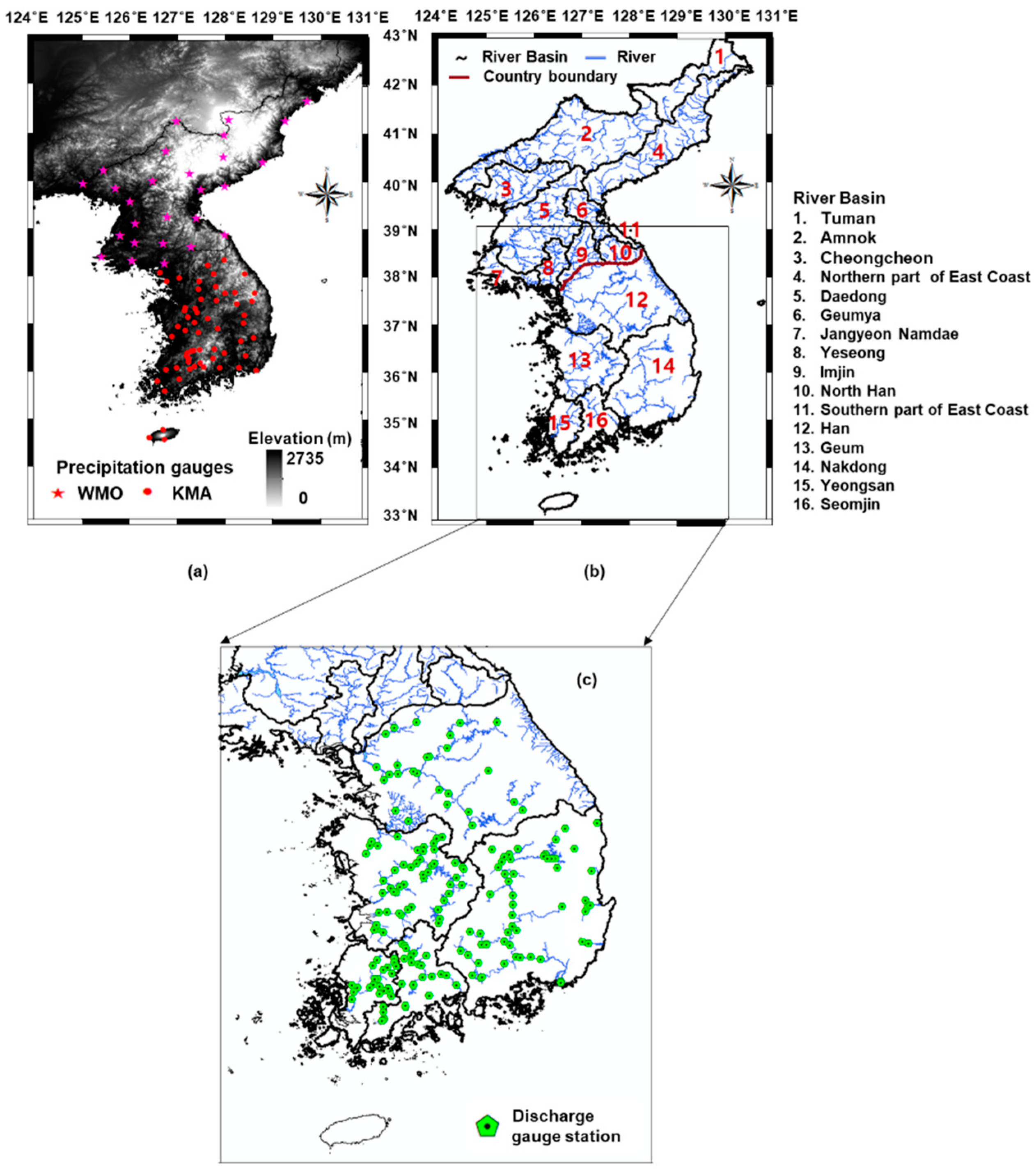
2.1. Study Area

The Korean Peninsula in Northeastern Asia is divided into two countries, namely South Korea (126°E–129°E, 33°N–38°N) and North Korea (124°E–131°E, 38°N–42°N). As indicated by the topographic data (DEM; digital elevation model) in Figure 1a, the Northern and Eastern parts are mountainous, whereas plains extend along the Western and Southern parts. The Korean Peninsula is affected by the East Asian monsoon—approximately 60–70% of the annual precipitation appears during the summer months [19]. An examination of Figure 1a also indicates that the World Meteorological Organization (WMO) has provided North Korea with 27 precipitation gauge stations, which is sparse compared to those provided by the Korea Meteorological Administration (KMA) in South Korea. In addition, Figure 1b indicates that the distribution of the river in the Korean Peninsula is relatively dense (0.2–0.5 km/km²), with most of the rivers flowing into the West Sea due to geographic characteristics. Many of the rivers have gentle slopes and wider basins, leading to higher amounts of discharge. There are eleven major river basins (1–10 in Figure 1b) in North Korea and five major river basins (11–16 in Figure 1b) in South Korea (

Table 1. Information of major river basins in the Korean Peninsula.

	River Basin	Area (km2)	Channel Reach (km)
North Korea	Tuman	10,290.7 (32,920.0) 1	547.8
	Amnok	33,367.2 (64,739.8) 1	803.0
	Cheongcheon	9368.2	217.0
	Northern part of East Coast	14,249.9	981.8
	Daedong	19,371.8	450.3
	Geumya	3365.7	145.1
	Jangyeon Namdae	1271.8	107.9
	Yeseong	3932.5	187.4
	Imjin	5113.5 (8129.5) 2	272.4
	North Han	3095.6 (10,834.0) 2	317.0
	Southern part of East Coast	535.6	70.6
South Korea	Han	26,219.0 (34,428.1) 3	483.0
	Geum	9914.0	388.0
	Nakdong	23,690.3	511.0
	Yeongsan	3469.6	135.0
	Seomjin	4914.3	222.0

Note: ¹ Basin area including China, ² basin area including South Korea and, ³ basin area including North Korea.

).

2.2. Independent Data

2.2.1. Terrestrial Water Storage Changes from the GRACE

The GRACE satellite system was launched by the National Aeronautics and Space Administration (NASA) with the objective of observing spatiotemporal variations in the Earth’s gravitational field. The time variance in the gravitational field detected by GRACE reflects the redistribution of the Earth’s water mass and can be converted to TWS changes after removing both the effects of nontidal (atmosphere and ocean) and tidal (solid Earth, ocean, and atmosphere). The gridded GRACE Level-2 RL05 datasets were processed by three organizations, namely: the Center for Space Research (CSR), the Jet Propulsion Laboratory (JPL), and the GeoForschungsZentrum (GFZ) using various orders of spherical harmonics to provide the gridded (1.0° × 1.0°) TWS anomaly (TWSA) data that were downloaded from the JPL Tellus site (http://grace.jpl.nasa.gov). The TWSA is the time mean value of the TWS (time span: January 2004 to December 2009) subtracted from the TWS using Equation (1) and can be used to compute the TWSC using Equation (2).

$${\mathrm{TWSA}}_i={\mathrm{TWS}}_i-\overline{\mathrm{TWS}}$$

(1)

$${\mathrm{TWSC}}_i=\frac{{\mathrm{TWSA}}_{i+1}-{\mathrm{TWSA}}_{i-1}}{2\mathsf{\Delta }t}$$

(2)

where $i$ is the month, $\overline{\mathrm{TWS}}$ is the average of the TWS, and $\mathsf{\Delta }t$ is the time span.

This study used the latest CSR RL05 data (

Table 2. Characteristics of data used in this study.

	Hydrologic Component	Data	Temporal Resolution	Spatial Resolution
Independent	TWSC	GRACE RL05	Monthly	1.0°
	Precipitation (P)	TMPA3B43		0.25°
	Soil moisture storage (SMS)	GLDAS_NOAH025_M
	Average temperature (T)
Dependent	Total discharge (Qtotal)	GLDAS_NOAH025_M	Monthly	0.25°
		Gauges *	Daily	Point
Validation	Total discharge (Qtotal)	GLDAS_NOAH025_M	Monthly	0.25°
		Gauges *	Daily	Point
		PRMS *		Local
		Water-balance method (Seo and Lee [11])	Monthly	1.0°

* Only available in South Korea TWSC: terrestrial water storage changes, GRACE: Gravity Recovery and Climate Experiment, TMPA: tropical rainfall measuring mission Multi-satellite Precipitation Analysis, GLDAS: global land data assimilation system, and PRMS: precipitation-runoff modeling system.

), which were provided by eliminated spherical harmonic coefficients at the order of 60 [20]. Although the RL05 data tend to reduce the retrieved TWSA amplitude due to destriping and smoothing, a multiplicative scaling factor can be applied to restore the signal attenuation [21]. To this end, scaling factors computed via the land TWSA time series output of the community land model (CLM) were applied to the RL05 TWSA dataset.

2.2.2. Precipitation from TRMM

One of the datasets provided by TRMM is the TRMM Multi-satellite Precipitation Analysis (TMPA), and the TMPA is provided at http://trmm.gsfc.nasa.gov. The TMPA 3B43 precipitation dataset was produced by incorporating the data of the TRMM satellite with data from the Special Sensor Microwave/Imager (SSM/I) sensor in the Defense Meteorological Satellite Program (DMSP) satellite, the advanced microwave scanning radiometer-Earth (AMSR-E) in the Aqua and National Oceanic and Atmospheric Administration (NOAA) satellites, and the global in situ precipitation measurement of the global precipitation climatology project (GPCP) produced by the NOAA’s Climate Prediction Center and Global Precipitation Climatology Center (GPCC). The TMPA 3B43 provides 0.25° (~25 km) monthly precipitation, covering 50°N to 50°S, 180°W to 180°E for 1998 to the present time. The TMPA dataset will continue by the next-generation global precipitation mission (GPM) satellite, although the TRMM satellite mission stopped in 2015. Previous studies demonstrated the applicability of the TMPA 3B43 to the Korean Peninsula by comparison with ground-based observations [22,23]. Hence, the TMPA 3B43 monthly precipitation data for the Korean Peninsula during the study period was extracted in this study (Table 2).

2.2.3. Soil Moisture Storage and Average Temperature from GLDAS

The GLDAS system produces primary land surface flux and storage component variables in water and energy cycles by forcing data from ground-based observations and satellites. Currently, the official website of GLDAS (http://ldas.gsfc.nasa.gov/gldas/) provides 3-h and monthly data with a spatial coverage of 0.25° and 1.0° by the application of widely used land surface models that have been well-proven in hydrometeorological fields, including the common land model (CLM), the mosaic, the Noah, and the variable inflatable capacity (VIC) models. Each model output is driven by various ground-based and satellite data and is modified by data assimilation. In view of the high accuracy of the model output demonstrated by previous studies, this is the primary source of data for hydrological analyses in ungauged areas around the world. For use in this study, the monthly GLDAS/Noah data for soil moisture (SMS) storage and average temperature (T) with a spatial resolution of 0.25° (GLDAS_NOAH025_M) were gathered from the NASA land information system and Goddard Earth Sciences Data and Information Services Center (GEDISC; Table 2). This contains four depth layers of soil moisture: 0–0.1 m (layer 1), 0.1–0.4 m (layer 2), 0.4–1.0 m (layer 3), and 1.0–2.0 m (layer 4), and soil moisture data were integrated for input data.

2.3. Dependent Data

The Water Management Information System (WAMIS), which is managed by the Korean government and the Korea Water Resources Corporation in South Korea, provides the discharge observations (http://www.wamis.go.kr/). Out of the 736 stations that have been operated up to 2016, 187 observation stations were adopted in this study for their data continuity and inclusion of the study period (2003–2016; Table 2). The gauge stations for discharge at the five major river basins (Han, Geum, Nakdong, Yeongsan, and Seomjin Rivers) are indicated in Figure 1c. Meanwhile, North Korea’s available hydrological data are limited to the precipitation data from a sparse 27 stations provided by the World Meteorological Organization (WMO; Figure 1a). In addition, the amount of discharge is difficult to estimate due to facility and operational problems, leading to poor reliability of the precipitation data. To overcome these problems, the GLDAS data were used to validate the total discharge over the Korean Peninsula by combining the surface and subsurface discharges. Thus, only the GLDAS total discharge data for North Korea, where no ground-based data existed, were used as the dependent data, while the GLDAS and ground-based discharge data for South Korea were combined via conditional merging techniques and used as the dependent data. A detailed description of the conditional merging technique is given in Section 3.3.

2.4. Validation Data

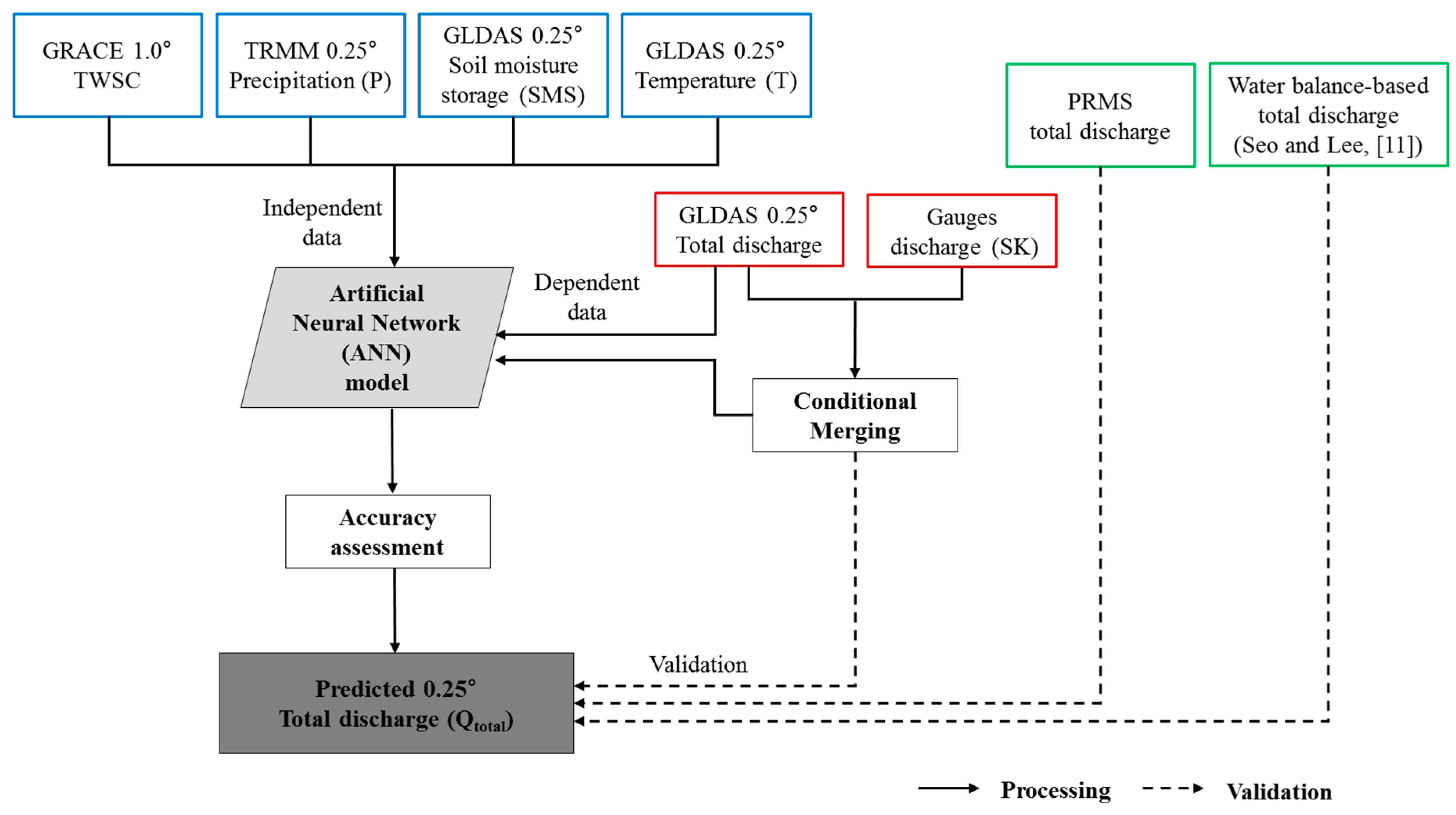
The GLDAS total discharge results were used as validation data. In addition, long-term total discharge data from the PRMS were used for South Korea. The PRMS model is a physics-based quasi-distributed effluent model developed by the U.S. Geological Survey (USGS) in 1983 and has been validated by several previous studies [24,25]. This model takes hydrologic interactions between the atmosphere, vegetation, and soil into account; subdivides the entire basin into homogeneous units termed hydrologic response units (HRU); and calculates the energy balance from these HRU to determine the outflow of the basin. The model is also known to simulate the surface water and intermediate and subsurface discharges [26]. The results of the PRMS analysis over 50 years (1966-2015) for the South Korea basins were provided by the WAMIS. The total discharge results for the Korean Peninsula obtained by Seo and Lee [11] based on the water balance was also used for validation data (Table 2). More details on this method are given in Section 3.1.

3. Methodology

The approach proposed in this study is represented by the process flow diagram in Figure 2. A total of four input variables were used to develop the total discharge prediction model, namely: GRACE TWSC, TRMM precipitation, GLDAS soil moisture storage, and average temperature. Taking the spatial resolution of other variables into consideration, the GRACE product was subsampled by dividing each 1.0° grid into uniform 0.25° sub-grids. The target variables were the total discharge from the GLDAS Noah model for the Korean Peninsula and the enhanced total discharge data obtained by combining the GLDAS and discharge gauge station data for South Korea (SK) via the conditional merging method. Then, the independent variables were fed into an ANN model to predict the downscaled total discharge (0.25°) for each target dataset. Validation was conducted to compare the performances of the total discharge data from GLDAS, gauges, PRMS, and the water balance results of Seo and Lee [11] and to rank the importance of the various input data.

3.1. Water Balance-Based Total Discharge

The water balance is based on the conservation of the water mass, also referred to as the continuity equation. Generally, the total discharge estimate is obtained using the terrestrial water balance equation [11]:

$${\mathrm{Q}}_{\mathrm{total}}=\left[\left(Q_{ro}+Q_{go}\right)-\left(Q_{ri}+Q_{gi}\right)\right]=\mathrm{P}-\mathrm{ET}-\mathrm{TWSC}$$

(3)

where ${\mathrm{Q}}_{\mathrm{total}}$ is the total discharge (mm/month), which involves the net of the surface and subsurface water flow, $Q_{ro}$ is the outflow of the surface water (mm/month), $Q_{go}$ is the outflow of the subsurface water (mm/month), $Q_{ri}$ is the inflow of the surface water (mm/month), $Q_{gi}$ is the inflow of the subsurface water (mm/month), P is the precipitation (mm/month), and ET is the actual evapotranspiration (mm/month).

Changes in the regional total discharge (${\mathrm{Q}}_{\mathrm{total}}$) can be evaluated by integrating the GRACE-measured TWSC with the precipitation and evapotranspiration observation data based on the terrestrial water balance. Seo and Lee [11] used the data from three satellites (GRACE, TRMM, and MODIS) to verify the feasibility of water balance-based ${\mathrm{Q}}_{\mathrm{total}}$ retrieval during the period January 2003–December 2014 in the Korean Peninsula. However, the water balance-based total discharge estimation raises uncertainties due to satellite data processes such as measurement error and the integration of each product. In the following, the total discharge results using the water balance based on multi-satellite data given by Seo and Lee [11] are used for validation of the ANN results of this study.

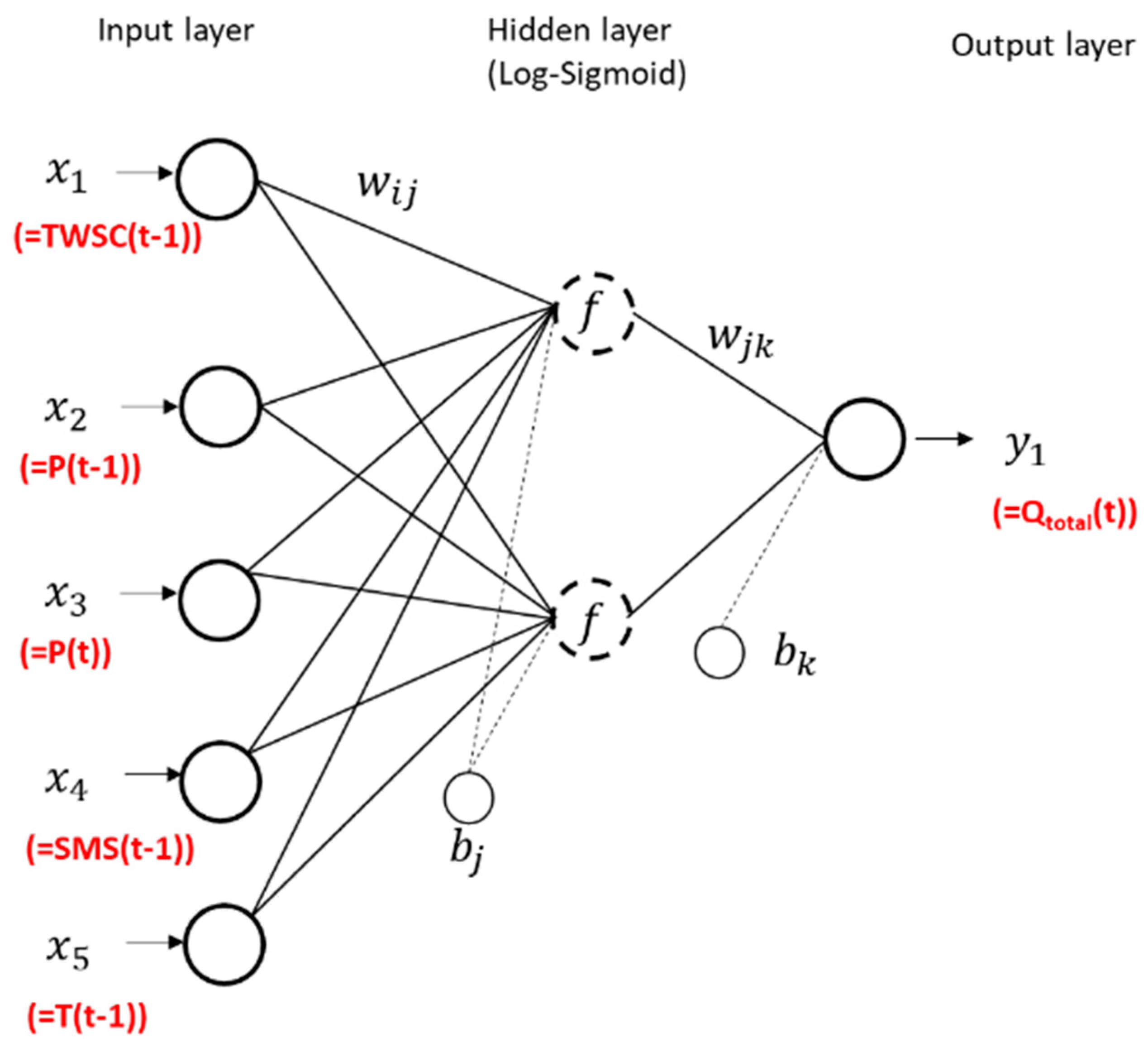
3.2. Artificial Neural Network

The ANN is widely used in machine learning as a data-driven approach that employs training algorithms [18]. The most common and typical training algorithm used in hydrological applications (e.g., prediction of rainfall, water level, and groundwater [14,15,16,17,18]) is the backpropagation algorithm with feed-forward nets. The ANN comprises nodes within input, hidden, and output layers, which form the units of basic computing, and each layer is connected by several links with assigned connection weights. The conventional ANN model is the multi-layer perceptron (MLP) with at least one hidden layer between the input and output layers that can flexibly interpret complex nonlinear relationships between independent and dependent variables.

The ANN learning process is performed according to Equations (4) and (5) below. When the input value set of $n$-dimensional vectors $\mathit{x}=\left[x_1,x_2,\dots ,x_n\right]$ is presented to the input layer, an output value set $\mathit{y}$ is computed through the hidden layer by applying the activation function $f$ and connection weight. The connection weights are updated by minimizing the error ($E$) between the predicted value ($y$) and target value ($t$) in accordance with Equation (6).

$$z_j=f\left({\displaystyle \sum }_i{w}_{ij}^1{x}_i+b_j\right)$$

(4)

$$y={\displaystyle \sum }_j{w}_{jk}^2{z}_j+b_k$$

(5)

$$E=\frac{1}{2}{(y-t)}^2$$

(6)

Here, the $w_{ij}^1$ is the connection weight between the input layer and hidden layer; $b_i$ is the bias term; $w_j^2$ is the connection weight between the hidden layer and output layer; $b_j$ is the bias; and $i$, $j$, and $k$ indicate the number of nodes in the input, hidden, and output layers, respectively.

3.2.1. Model Setup

The above-mentioned ANN machine-learning approach was used to predict the 0.25° total discharge data. The GRACE TWSC, TRMM precipitation (P), GLDAS average temperature (T), and GLDAS soil moisture (SMS) were processed over the Korean Peninsula in order to make up a prediction model. A total of 63,168 samples (168 months × 376 pixels) were obtained for the Korean Peninsula, and these were used to develop the ANN models. The feed-forward ANN MLP model with a backpropagation algorithm was used in this study. As shown in Figure 3, the input data for the ANN model consisted of monthly TWSC, P, SMS, and T. As previously explained, three tests were designed according to the target data, as listed in

Table 3. Input data and target data corresponding to test cases. P: precipitation, T: average temperature, SMS: soil moisture, and IDW: inverse distance weighting.

	Input Data	Target Data	Study Area (no. samples)	No. Neurons of Hidden Layer
Case I	TWSC+P+SMS+T	Qtotal (GLDAS)	Korean peninsula (376 × 168)	1~10
Case II		Qtotal (GLDAS+gauges (IDW))	South Korea (163 × 168)
Case III		Qtotal (GLDAS+gauges (Kriging))

. Thus, for Case I, the target data were the total discharge over the Korean Peninsula from the GLDAS Noah model, whereas Cases II and III were based on the combined GLDAS and gauged discharge interpolated data for South Korea by using the conditional merging method along with the inverse distance weighting (IDW; Case II) and Kriging methods (Case III).

The caveat in ANN configurations is that overfitting or the generation of a local minimum can occur due to the complex computational processes and structures. Therefore, it is essential to choose an appropriate training algorithm and an appropriate number of nodes on the hidden layer. In addition, it is essential to determine an activation function to run the ANN model, which is converting the input signal of nodes to the output signal.

Hence, the Levenberg-Marquardt algorithm [27], which is based on the Gauss-Newton approximation and is generally used for training purposes [28], was applied to the ANN model in this study. The Levenberg-Marquardt algorithm has the advantage of converging faster and more reliably than the majority of training algorithms [27]. The epoch for the training was assigned to 1000, and early stop criteria were defined to avoid overfitting and to enhance the generalization of the ANN model. The training was stopped if the target value of error in the training set was met or when the error gradient reached a minimum threshold. As shown in Table 3, the number of nodes on the hidden layer was varied from 1 to 10 in order to calculate the optimum number, considering the computing demand. The structure of the ANN model used in this study is shown in Figure 3, where $f$ refers to the log-sigmoid activation function that is frequently used for ANN training. The time scale was divided into three parts, consisting of the training (60%; 2003.01–2011.04; 100 months), validation (20%; 2011.05–2014.02; 34 months), and test periods (20%; 2014.03–2016.12; 34 months).

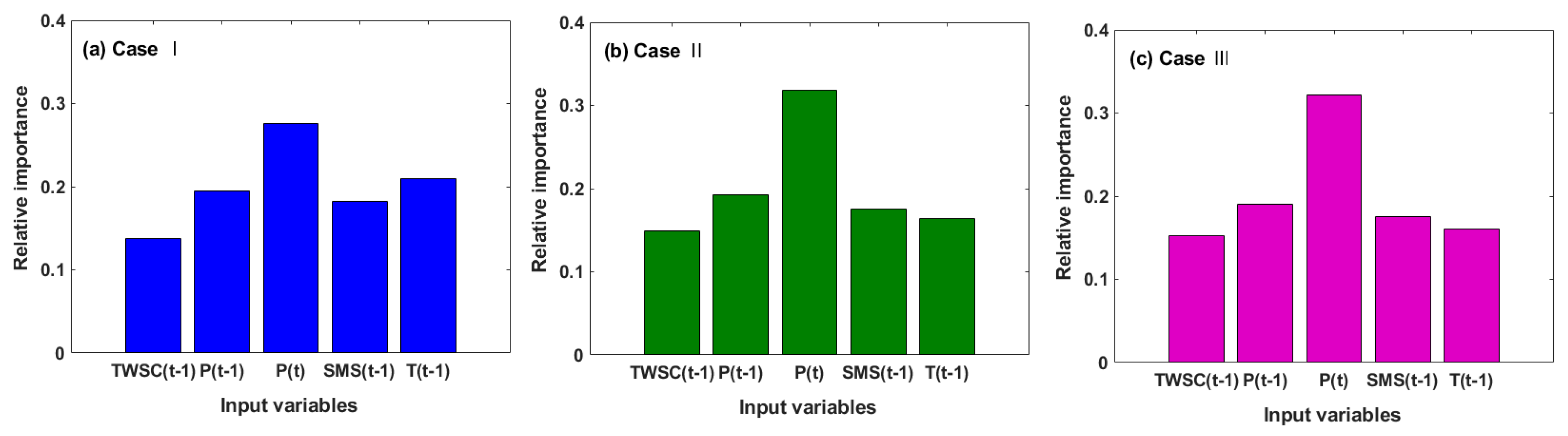
3.2.2. Sensitivity Analysis

The general objective of the sensitivity analysis in ANN models is to evaluate the relative importance of the independent data. It is necessary to understand whether the predictions of the developed ANN model are similar to real-world phenomena and whether a valid relation between the input and output data has been applied. A method proposed by Olden et al. [29] for determining the relative importance of input variables in neural networks is similar to the Garson algorithm [30], in that it uses connection weights. Garson’s algorithm considers only the absolute magnitude of the connection weight, while the Olden method considers both the magnitude and sign (positive or negative) to analyze the response between input and output data in more detail. Thus, the Olden method can be applied not only to a single hidden layer but, also, to the multi-hidden layer ANN model [29,31].

As shown in Figure 3, the application of the Olden connection weight method proceeds in three steps [29]. First, the input-hidden connection weight ($w_{ij}^1$) and the hidden-output connection weight ($w_j^2$) between the input and output nodes are multiplied to give a product matrix $Q_i$ and then, the product is summed ($S_i$) as the product across all hidden nodes. The relative importance ($R{I}_i$) of the $i$th input variable is then defined by Equation (7):

$$R{I}_i=\frac{S_i}{{\displaystyle \sum }{S}_i}$$

(7)

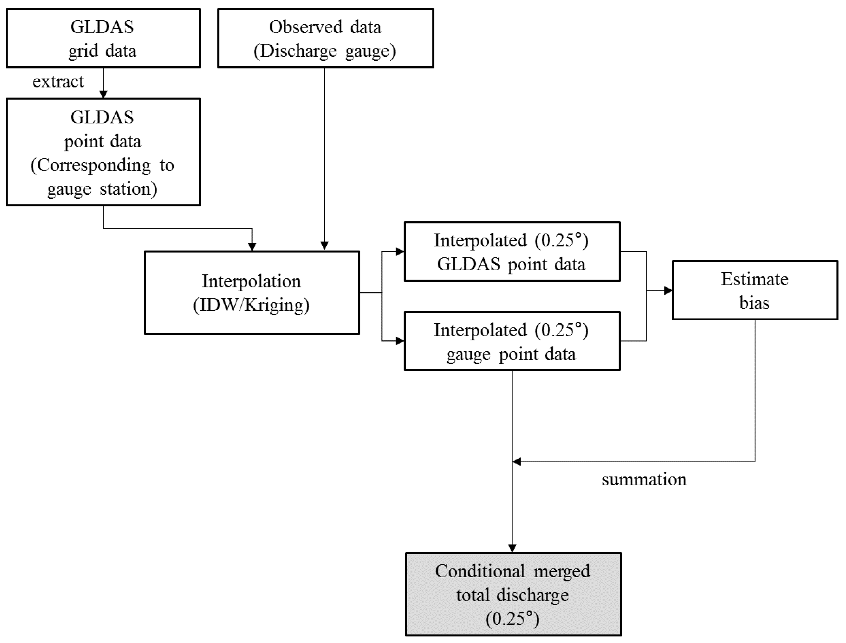
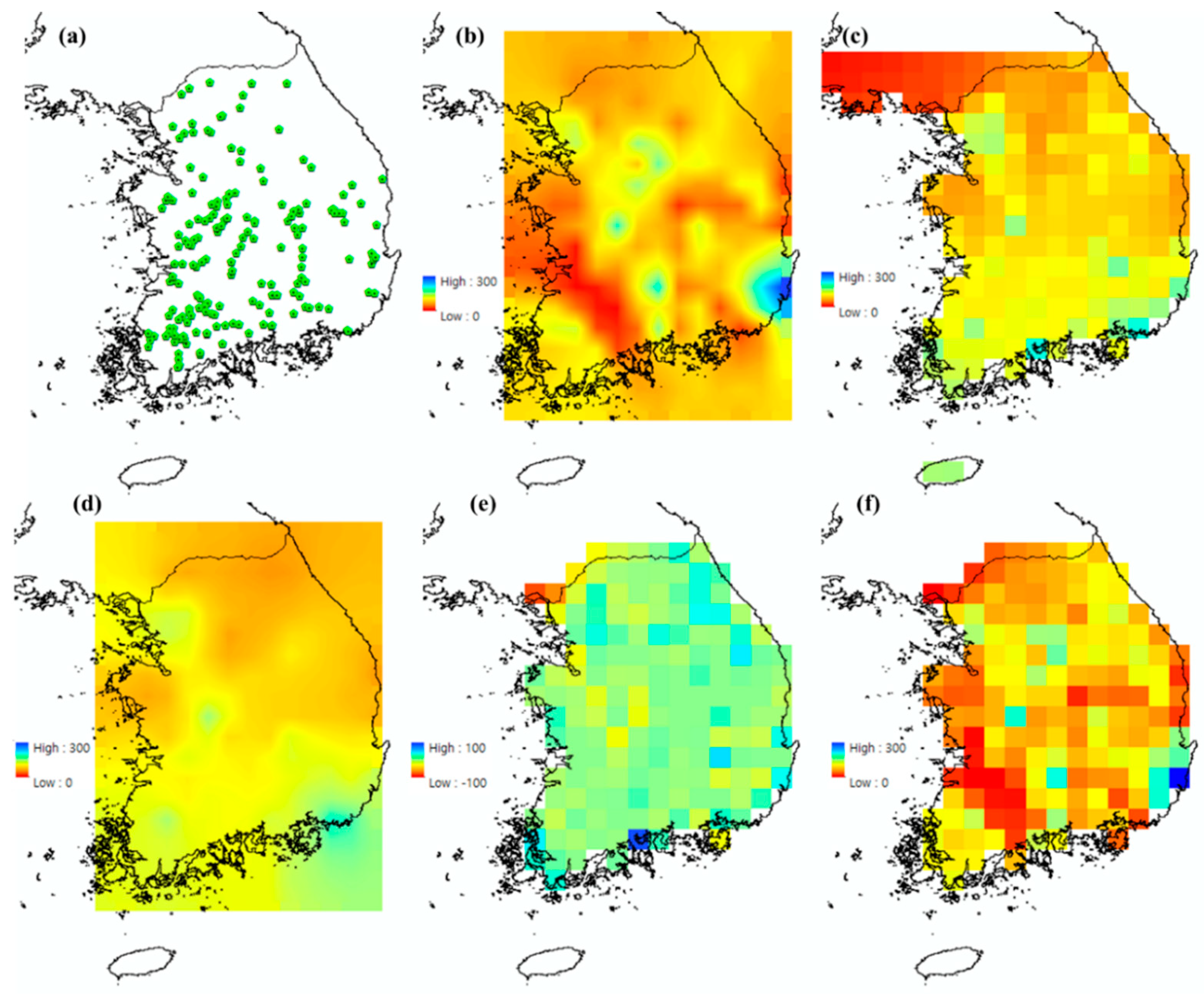
3.3. Conditional Merging

The conditional merging method, otherwise known as the kriging error correction method, is a strategy for merging satellite and ground-based observation data that was introduced by Ehret [32] and Sinclair and Pegram [33]. This method has been used to overcome the limitations of ground-based observations with point data while maintaining the accuracy of the ground data along with the spatially continuous data from satellites. Therefore, the spatial correlation of each dataset and the heterogeneity of the data can be identified [34]. Early studies using the conditional merging of precipitation data from radar and gauge sources demonstrated improved spatial and temporal variability. Recently, the conditional merging method has been applied in a wide scope of hydrological studies, including soil moisture [35] and land surface temperature [36]. In this study, the conditional merging method was used to obtain improved total discharge data from GLDAS and gauge discharge data, which were then used as the dependent variables for South Korea. In addition, the ArcGIS tool was used for interpolator IDW and Kriging (ordinary Kriging with an exponential semi-variogram model).

As indicated in Figure 4 and Figure 5, this process involved the following steps: (a) the observed discharge at 187 stations across South Korea were collected, (b) the interpolation field (0.25°) was computed using either the IDW (Case II) or the Kriging (Case III) interpolator from the station data, (c) the values corresponding to the station used in step (a) were extracted from the GLDAS grid cells, (d) the 0.25° interpolation field was estimated by applying either the IDW (Case II) or Kriging (Case III) to the grid cells extracted in step (c), (e) the residual between (b) and (d) was estimated, and (f) the merged 0.25° total discharge field was obtained by adding the residual field from (e) to the interpolation field (0.25°) from the ground-based discharge data in step (a).

3.4. Metrics for Evaluation

In this study, the performance of the ANN models for predicting the total discharge was evaluated using statistical indicators such as the correlation coefficient (r; Equation (8)), maximum absolute error (MAE; Equation (9)), root mean square error (RMSE; Equation (10)), and Nash–Sutcliffe efficiency (NSE; Equation (11)). The r is an indicator of the degree of linearity in the interconnection between the prediction and observation; the r value is closer to 1; there is the positive correlation between the two datasets. Meanwhile, the MAE and RMSE provide measurements of the error. The closer the MAE and RMSE are to 0, the less is the error. Finally, the Nash-Sutcliff efficiency (NSE) measures the ability of the prediction of a model relative to the mean of the observation ranges between (−∞, 1) and measures, where a value of 1 indicates a perfect match between the datasets, a value of 0 indicates that the predictions similar as the average of the observed data, and a negative value indicates that the mean of the observation is more similar than the model.

$$r=\frac{{\displaystyle {\displaystyle \sum }_{i=1}^N}\left(X_i-\bar{X}\right)\left(Y_i-\bar{Y}\right)}{\sqrt{{\displaystyle {\displaystyle \sum }_{i=1}^N}{\left(X_i-\bar{X}\right)}^2{\displaystyle {\displaystyle \sum }_{i=1}^N}{\left(Y_i-\bar{Y}\right)}^2}}$$

(8)

$$\mathrm{MAE}=\frac{1}{N}{\displaystyle \sum }_{i=1}^N\left|X_i-Y_i\right|$$

(9)

$$\mathrm{RMSE}=\sqrt{\frac{1}{N}{\displaystyle \sum }_{i=1}^N{\left(X_i-Y_i\right)}^2}$$

(10)

$$\mathrm{NSE}=1-\frac{{\displaystyle {\displaystyle \sum }_{i=1}^N}{\left(Y_i-X_i\right)}^2}{{\displaystyle {\displaystyle \sum }_{i=1}^N}{\left(X_i-\bar{X}\right)}^2}$$

(11)

where $X$ is the observed data, $\bar{X}$ is the mean of $X$, $Y$ is the predictive data, $\bar{Y}$ is the mean of $Y$, and $N$ is the number of data.

4. Results

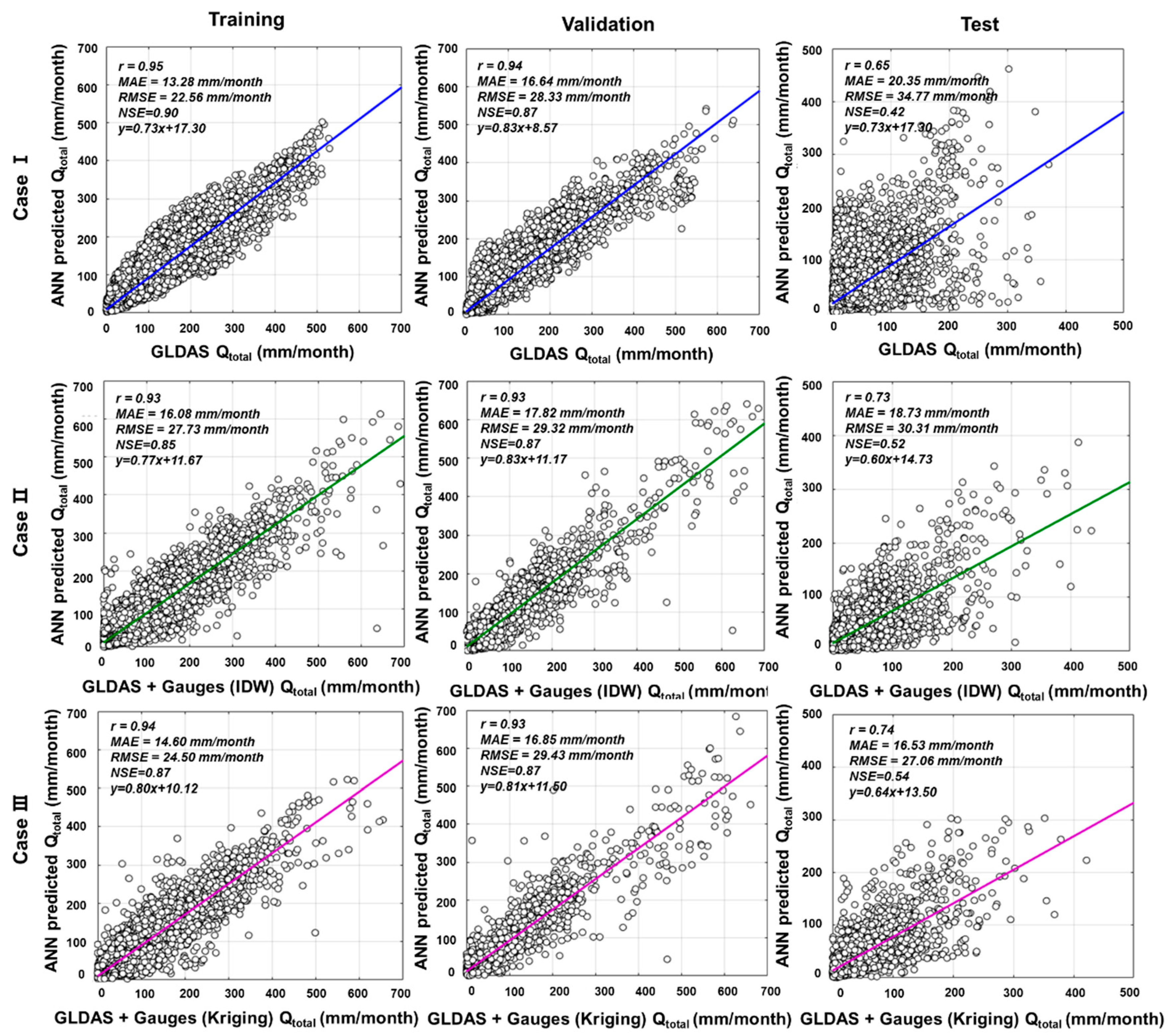
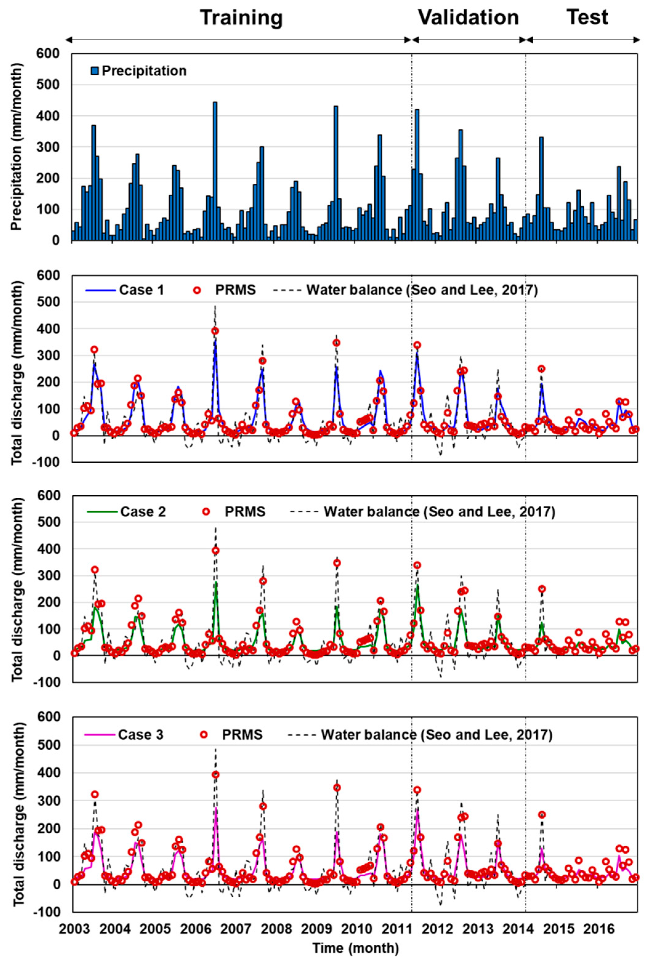
4.1. ANN-Predicted Total Discharge

The results of ANN modelling to predict the downscaled total discharge using the various satellite and reanalysis products are presented in Figure 6, where each row represents a specific case, and each column represents the results of each period (training, validation, and test). A total of the backpropagation algorithm was trained at 1000 epochs through 100 iterations, and the predictions indicated the most accurate results when the number of nodes on the hidden layer was set to four.

Among the three cases, Case III resulted in the best performance in the test period (2014.03-2016.12), with r = 0.74, MAE = 16.53 mm/month, RMSE = 27.06 mm/month, and NSE = 0.54 for South Korea. Similar to Case III, Cases I and II produced relatively good performances (r = 0.65–0.95, MAE = 13.28–20.35 mm/month, RMSE = 22.56–34.77 mm/month, and NSE = 0.42–0.90). Thus, the ANN method was able to produce relatively accurate models for the total discharge, which resulted in positive slopes.

The correlation between the ANN-predicted total discharge and target data was examined for each case. The spatial distributions of the RMSE, r, and NSE between the target total discharge and ANN-predicted total discharge over the test period (2014.03–2016.12) are presented in Figure 7. Overall, a low RMSE is noted in each case (blue color; first column in Figure 7), whereas the RMSE in North Korea is higher than that of South Korea. In addition, certain Eastern and Southern coastal regions in South Korea and the border area between South and North Korea display higher RMSE values (red color; first column in Figure 7). Moreover, positive correlations (blue color; second column in Figure 7) are observed in most areas. Similarly, the overall NSE results are fairly accurate (blue color; third column in Figure 7), although a lower accuracy is indicated in the Western regions of North Korea. In Cases II and III, a low NSE value is observed in the border regions. In the Coastal regions, the satellite or reanalysis data have uncertainties caused by tidal effects; there is a higher degree of error than other areas. In addition, these regions have a lack of ground observations. For these reasons, it appears to indicate low correlations and high errors.

As indicated in Figure 8, the P(t) was identified by the ANN as being the most important input parameter for all three cases: I, II, and III, while the TWSC appeared to be the least important. As shown in Figure 8a, the relative importance of each parameter for Case I was P(t) at 0.276, followed by T(t-1) (one month ahead) at 0.210, P(t-1) at 0.195, SMS(t-1) at 0.182, and TWSC(t-1) at 0.137, thus indicating comparable levels of importance for each factor. In Case II, the relative importance was 0.318 for the P(t), followed by the 0.193 for P(t-1), 0.176 for SMS(t-1), 0.164 for T(t-1), and 0.149 for TWSC(t-1) (Figure 8b). Similarly, the P(t) was of the highest importance in Case III at 0.321, followed by P(t-1) at 0.190, SMS(t-1) at 0.175, T(t-1) at 0.161, and TWSC(t-1) at 0.153 (Figure 8c). Thus, in all three cases, the P(t) and P(t-1) were identified as being very useful for the prediction of the total discharge, followed by the SMS and T. Total discharge is one of the key controls of water flux and is closely linked to precipitation. However, since these values are similar to each other, the present results demonstrate that all input data have a noteworthy effect on the total discharge prediction.

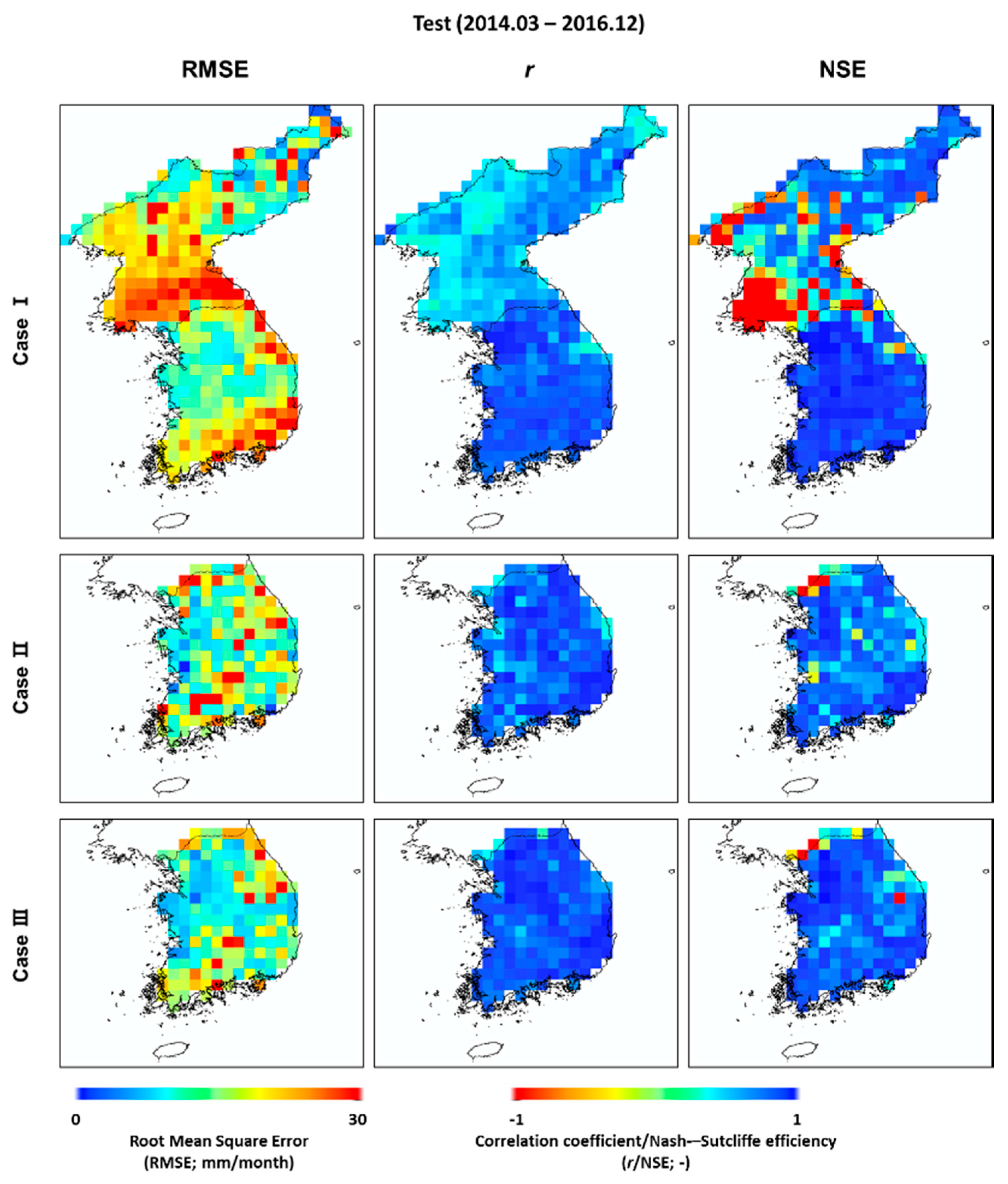
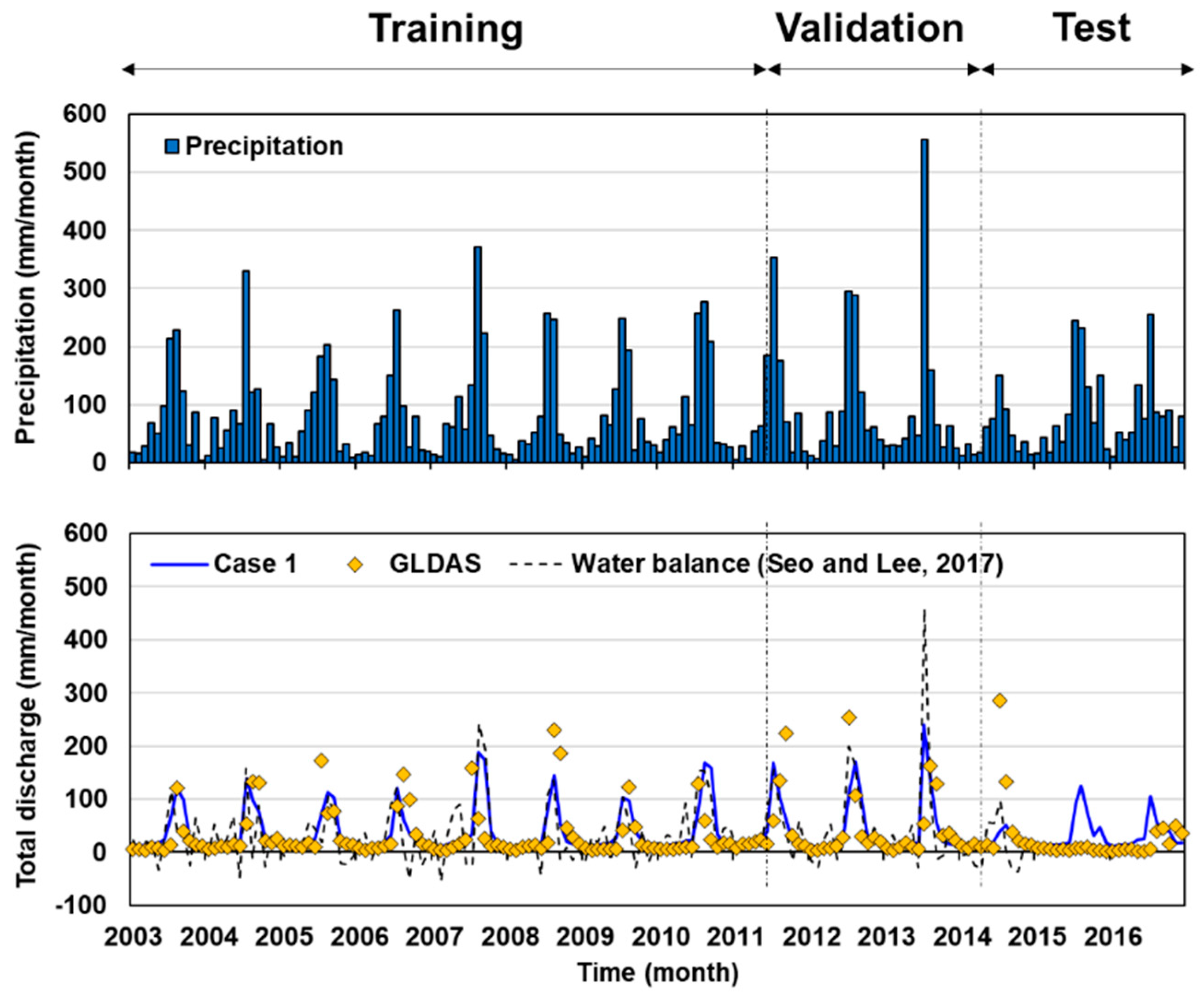
4.2. Validation of ANN-Predicted Total Discharge

The monthly time series of the ANN-predicted total discharge at 0.25° scales (Cases I, II, and III); PRMS total discharge; and water balance-based total discharge according to Seo and Lee [11], corresponding to the precipitation in South Korea, are presented in Figure 9. The vertical two lines indicate the partition between the training (2003.01–2011.04), validation (2011.05–2014.02), and test periods (2014.03–2016.12).

The top panel presents the precipitation results from 56 stations in the KMA (Figure 1a), while the second, third, and fourth panels (Figure 9) present the results of Case I, Case II, and Case III, respectively, for South Korea, compared with the PRMS and water balance results from Seo and Lee [11]. In the Korean Peninsula, most of annual precipitation falls during July to September due to the monsoon, and the ANN-predicted total discharge starts to fluctuate in May and peaks in the summer season. Thus, the ANN-predicted total discharge closely matches the observed fluctuations in the precipitation. Moreover, the ANN-predicted total discharge is well-correlated with the dynamics of the PRMS and water balance total discharge data (r = 0.86–0.96). In all three cases, the ANN model tends to overestimate the water balance-based total discharge compared to the PRMS. In particular, the test results (March 2014–December 2016), which provide an independent ANN estimation and have no influence on the training/validation procedure, indicate that the ANN-predicted total discharge is closely correlated to the PRMS and water balance-based data.

The ANN-predicted total discharge (Case I), GLDAS, and water balance-based total discharge corresponding to precipitation in North Korea are shown in Figure 10. Overall, the total discharge of North Korea is lower than that of South Korea, and the GLDAS data tend to be underestimated compared to other data. In particular, it was found that there was little total discharge regardless of precipitation during the test period. However, the ANN-predicted and water balance-based total discharges displayed seasonal trends according to the precipitation. This is thought to be the cause for the low correlation and the high RMSE for the North Korean region in Case I (Figure 7). However, Case I showed a more reasonable correspondence with the water balance-estimated total discharge than with the GLDAS total discharge.

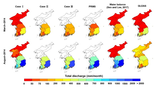
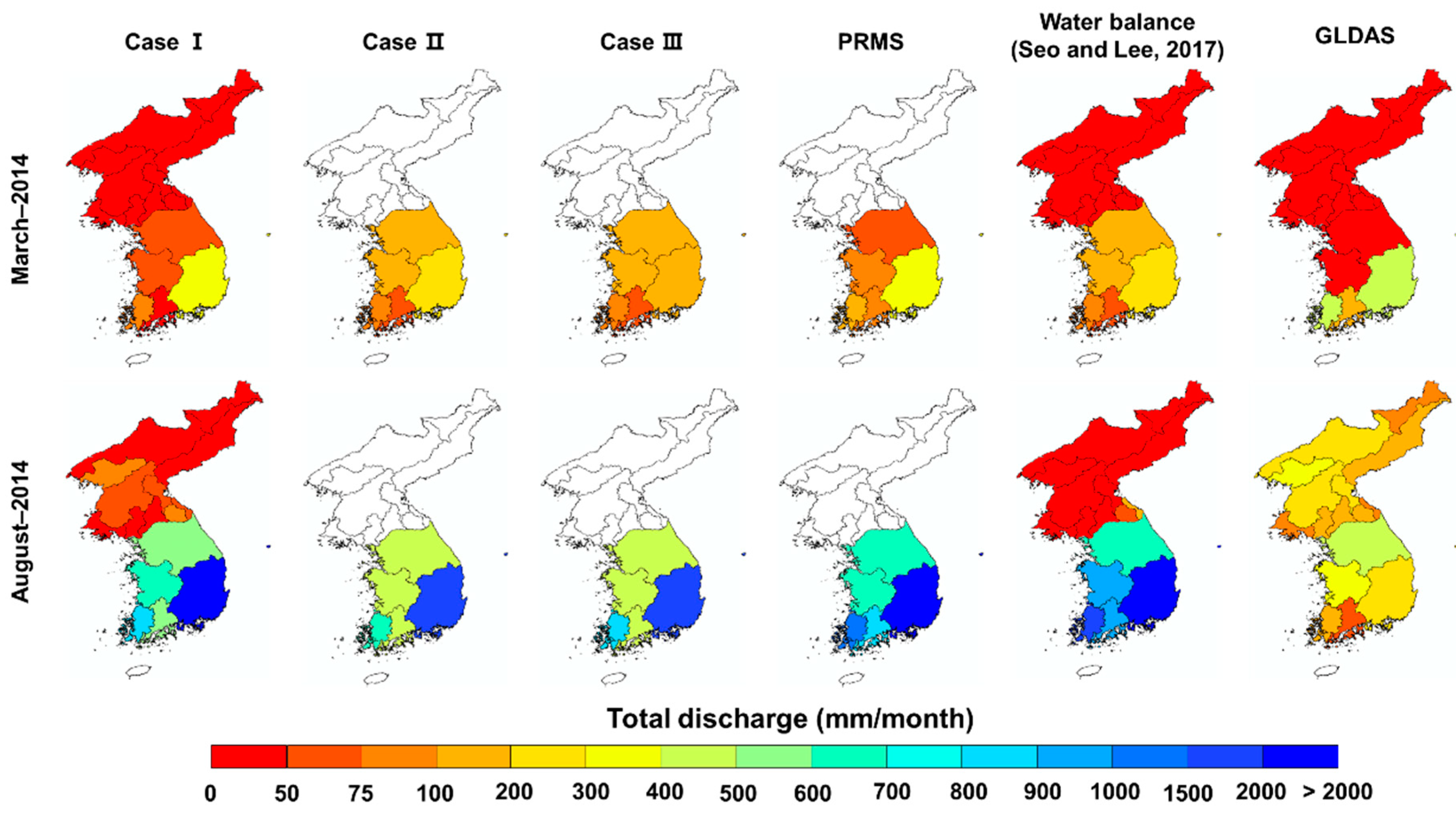
4.3. Spatial Distribution of Total Discharge

The ANN-predicted total discharges (Cases I, II, and III) are compared with the PRMS, water balance-estimated, and GLDAS total discharges for March 2014 and August 2014 for the major basins of the Korean Peninsula in Figure 11. Here, the ANN-predicted total discharge shows similar spatial patterns compared to the PRMS and water balance-based total discharges, whereas the GLDAS underestimates the total discharge with a smaller dynamic range than the other models. In addition, the water balance-based total discharge produces comparatively higher results. Furthermore, a visual comparison of the total discharge patterns by site (North Korea and South Korea), model, and month confirms that the ANN-predicted total discharge shows the best visual agreement with the PRMS overall, whereas the GLDAS cannot capture the high total discharge well.

The average annual precipitation and total discharge results for all major basins (Han, Geum, Nakdong, Yeongsan, and Seomjin Rivers) of South Korea are compared in Figure 12. Here, the results show similar patterns of variations in the total discharge depending on the dynamic variations in the precipitation. Thus, the ANN-predicted average annual total discharges are 633.7 mm/yr (95% confidence interval: 565.37–702.23 mm/yr) for Case I, 509.97 mm/yr (95% confidence interval: 457.10–562.04 mm/yr) for Case II, and 501.12 mm/yr (95% confidence interval: 448.56–553.69 mm/yr) for Case III, while the PRMS average annual total discharge is 723 mm/yr (95% confidence interval: 616.82–830.56 mm/yr), and the water balance-based result is 1090.40 mm/yr (95% confidence interval: 980.96–1199.83 mm/yr). As shown in Figure 11, the PRMS and ANN-predicted total discharges (especially in Case I) are similar, whereas the water balance-based total discharge result is slightly higher than in other models.

Similarly, the average annual precipitation and total discharge results for the major basins in North Korea (Tuman, Amnok, Cheongcheon, the Northern and Southern parts of the East Coast, Daedong, Geumya, Jangyeon Namdae, Yeseong, Imjin, and North Han Rivers) are presented in Figure 13. Hence, the precipitation and total discharge are comparatively lower than in South Korea. In detail, the ANN-predicted annual total discharge for Case I is 453.45 mm/yr 95% confidence interval: 405.70–501.20 mm/yr), while the GLDAS result is 396.23 mm/yr (95% confidence interval: 314.61–477.85 mm/yr), and the water balance-based result is 731.19 mm/yr (95% confidence interval: 622.59–839.79 mm/yr). Thus, as in Figure 11, similar values are obtained for Case I, GLDAS, and the water balance-based total discharge, although the GLDAS result is comparatively lower than the ANN-predicted result, and the water balance-based result is comparatively higher than the ANN prediction.

5. Conclusions

The potential to monitor water storage variations by remote sensing was examined herein. In particular, the prediction of changes in water bodies (e.g., discharge, soil moisture, groundwater, etc.) was conducted by merging various fusion datasets from multi-satellites, reanalysis data, and ground-based observations via machine learning. The ANN machine-learning approach was evaluated for the prediction of the downscaled (0.25°) total discharge in the Korean Peninsula using the TWSC from the GRACE satellite, the precipitation from the TRMM satellite, and the soil moisture storage and the average temperature from the GLDAS model. Since there was no hydrological information for the ungauged area in North Korea, target data were set to GLDAS data only for Case I, whereas the total discharge data for Cases II and III were obtained by conditional merging of the GLDAS and discharge gauge data.

The ANN approach used in this study was shown to be suitable for predicting the total discharge. The simulation results showed relatively good performance, leading to high r values of ~0.65–0.95, MAEs of ~13.28–20.35 mm/month, RMSEs of ~22.56–34.77 mm/month, and NSEs of ~0.42–0.54. For the test period, Case III showed the best performance in terms of the MAE, RMSE, r, and NSE. Among the four input variable products, precipitation was identified as being significantly the most important variable for predicting the total discharge in all three cases of the ANN model. However, the ANN-predicted total discharge displayed high error and low accuracy for the target data in coastal regions of North Korea and border regions due to the lack of information in these ungauged areas.

The predicted total discharge data with 0.25° resolution yielded a higher correlation between the PRMS (for Cases II and III) and the water balance-based total discharge from Seo and Lee [11] than with the GLDAS. The GLDAS provided lower total discharge results than the other models. The temporal variations in the total discharge showed similar patterns to those observed in response to variations in the precipitation. The ANN-predicted total discharge maps presented in Figure 11 revealed a higher total discharge in South Korea than in North Korea. While this study revealed the potential of the ANN approach for predicting the total discharge data, including ungauged areas, there were several limitations. Since the GRACE product of the input data were only available in monthly temporal resolutions, the temporal variations in the ANN-predicted data could not be modeled precisely. In addition, the multi-satellite and reanalysis data had relatively low spatial resolutions, and improvements in the resolutions are needed.

Nevertheless, this preliminarily test of the ANN approach has demonstrated its promise for the prediction of the total discharge based on data fusion from multi-satellites, reanalysis data, and ground observations. However, there are some challenges in the ANN approach, such as determining the optimal input parameters, physical-based issues, and generalization problems [37]. The development of strategies and methodologies are needed for improving the performance of ANN through further research.

Since GRACE stopped working in 2017, it has been replaced by the next generation, the GRACE Follow-On (GRACE-FO) mission. In addition, there is a precipitation-measuring satellite—namely, the global precipitation measurement (GPM) satellite network—following on from the TRMM. Hence, the approach proposed in this study should be further expanded and should utilize these newer satellites for information.

The total discharge is considered to be one of the key factors in water hazards such as droughts and floods, the ANN-predicted total discharge in this study can provide alternative tools instead of complex physical modeling and valuable information for local-to-regional hydrological managements, including those of ungauged areas.

References

1. Wagner, T.; Sivapalan, M.; Troch, P.; Woods, R. Catchment classification and hydrologic similarity. Geogr. Compass. 2007, 1, 901–931. [Google Scholar] [CrossRef]
2. Sayama, T.; Mcdonnell, J.J.; Dhakal, A.; Sullivan, K. How much water can a watershed store? Hydrol. Process. 2011, 25, 3899–3908. [Google Scholar] [CrossRef]
3. Hannah, D.M.; Demuth, S.; van Lanen, H.A.J.; Looser, U.; Prudhomme, C.; Rees, G.; Stahl, K.; Taallaksen, L.M. Large-scale river flow archives: Important, current status and future needs. Hydrol. Process. 2011, 25, 1191–1200. [Google Scholar] [CrossRef]
4. McCabe, M.F.; Rodell, M.; Alsdorf, D.E.; Miralles, D.G.; Uijlenhoet, R.; Wagner, W.; Lucieer, A.; Houborg, R.; Verhoest, N.E.C.; Franz, T.E.; et al. The future of earth observation in hydrology. Hydrol. Earth Syst. Sci. 2017, 21, 3879–3914. [Google Scholar] [CrossRef] [Green Version]
5. Sheffield, J.; Wood, E.F.; Pan, M.; Beck, H.; Coccia, G.; Serrat-Capdevilla, A.; Verbist, K. Satellite remote sensing for water resources management: Potential for supporting sustainable development in data-poor regions. Water Resour. Res. 2018, 54, 9724–9758. [Google Scholar] [CrossRef] [Green Version]
6. Rodell, M.; Velicogna, I.; Famiglietti, J.S. Satellite-based estimates of groundwater depletion in India. Nature 2009, 460, 999–1002. [Google Scholar] [CrossRef] [PubMed] [Green Version]
7. Famiglietti, J.S.; Lo, M.; Ho, S.L.; Bethune, J.; Anderson, K.J.; Syed, T.H.; Swenson, S.C.; de Linage, C.R.; Rodell, M. Satellites measure recent rates of groundwater depletion in California’s Central Valley. Geophys. Res. Lett. 2011, 38, L03403. [Google Scholar] [CrossRef] [Green Version]
8. Scanlon, B.R.; Faunt, C.C.; Longuevergne, L.; Reedy, R.C.; Alley, W.M.; McGuire, V.L.; McMahon, P.B. Groundwater depletion and sustainability of irrigation in the US High Plains and Central Valley. Proc. Natl. Acad. Sci. USA 2012, 109, 9320–9325. [Google Scholar] [CrossRef] [Green Version]
9. Buma, W.G.; Lee, S.-I.; Seo, J.Y. Hydrological evaluation of Lake Chad Basin using space borne and hydrological model observations. Water 2016, 8, 205. [Google Scholar] [CrossRef] [Green Version]
10. Seo, J.Y.; Lee, S.-I. Integration of GRACE, ground observation, and land-surface models for groundwater storage variations in South Korea. Int. J. Remote Sens. 2016, 37, 5786–5801. [Google Scholar] [CrossRef]
11. Seo, J.Y.; Lee, S.-I. Total discharge estimation in the Korean Peninsula using multi-satellite products. Water 2017, 9, 532. [Google Scholar] [CrossRef] [Green Version]
12. Houborg, R.; Rodell, M.; Li, B.; Reichle, R.; Zaitchik, B.F. Drought indicators based on model-assimilated Gravity Recovery and Climate Experiment (GRACE) terrestrial water storage observations. Water Resour. Res. 2012, 48, W07525. [Google Scholar] [CrossRef] [Green Version]
13. Choi, C.; Kim, J.; Han, H.; Han, D.; Kim, H.S. Development of water level prediction models using machine learning in wetlands: A case study of Upo wetland in South Korea. Water 2019, 12, 93. [Google Scholar] [CrossRef] [Green Version]
14. Sun, A. Predicting groundwater level changes using GRACE data. Water Resour. Res. 2013, 49, 1–13. [Google Scholar] [CrossRef]
15. Young, C.-C.; Liu, W.-C. Prediction and modelling of rainfall-runoff during typhoon events using a physically-based and artificial neural network hybrid model. Hydrol. Sci. J. 2013, 60, 2102–2116. [Google Scholar] [CrossRef]
16. Seo, J.Y.; Lee, S.-I. Spatio-temporal groundwater drought monitoring using multi-satellite data based on an artificial neural network. Water 2019, 11, 1953. [Google Scholar] [CrossRef] [Green Version]
17. Vu, M.T.; Aribarg, T.; Supratid, S.; Raghavan, S.V.; Liong, S.-Y. Statistical downscaling rainfall using artificial neural network: Significantly wetter Bangkok? Theor. Appl. Climatol. 2016, 126, 453–467. [Google Scholar] [CrossRef]
18. Tarpanelli, A.; Santi, E.; Tourian, M.J.; Filippucci, P.; Amarnath, G.; Brocca, L. Daily river discharge estimates by merging satellite optical sensors and radar altimetry through artificial neural network. IEEE Trans. Geosci. Remote Sens. 2019, 57, 329–341. [Google Scholar] [CrossRef]
19. Ghafouri-Azar, M.; Bae, D.-H.; Kang, S.-U. Trend analysis of long-term reference evapotranspiration and its components over the Korean Peninsula. Water 2018, 10, 1373. [Google Scholar] [CrossRef] [Green Version]
20. Landerer, F.W.; Swenson, S.C. Accuracy of scaled GRACE terrestrial water storage estimates. Water Resour. Res. 2012, 48, W04531. [Google Scholar] [CrossRef]
21. Swenson, S.C. GRACE Monthly Land Water Mass Grids NETCDF RELEASE 5.0. Ver. 5.0; PO.DAAC: Santa Rosa, CA, USA, 2012. [Google Scholar]
22. Koo, M.S.; Hong, S.Y.; Kim, J. An evaluation of the tropical rainfall measuring mission (TRMM) multi-satellite precipitation analysis (TMPA) data over South Korea. Asia-Pac. J. Atmos. Sci. 2009, 45, 265–282. [Google Scholar]
23. Sohn, B.J.; Han, H.-J.; Seo, E.-K. Validation of satellite-based high-resolution rainfall products over the Korean Peninsula using data from a dense rain gauge network. J. Appl. Meteorol. Clim. 2010, 49, 701–714. [Google Scholar] [CrossRef]
24. Kim, N.W.; Kim, H.J.; Park, S.H. Long-term runoff characteristics on HRU variations of PRMS. J. Korea Water Resour. Assoc. 2005, 38, 167–177. [Google Scholar] [CrossRef] [Green Version]
25. Jung, I.W.; Bae, D.-H. A study on PRMS applicability for Korean River Basin. J. Korea Water Resour. Assoc. 2005, 38, 713–725. [Google Scholar] [CrossRef]
26. Baek, K.; Lim, D. Study on Evaluating Low Flow in Ungauged Basin; Report on Gyeonggi Research Institute: Gyeonggi-do, Korea, 2010; pp. 1–178. [Google Scholar]
27. Hao, Y.; Wilamowski, B.M. Levenberg-Marquardt Training, Industrial Electronics Handbook, Intelligent Systems, 2nd ed.; CRC Press: Boca Raton, FL, USA, 2011; pp. 12-1–12-15. [Google Scholar]
28. Björck, A. Numerical Methods or Least Squares Problems; Society for Industrial and Applied Mathematics: Philadelphia, PA, USA, 1996. [Google Scholar]
29. Olden, J.D.; Joy, M.K.; Death, R.G. An accurate comparison of methods for quantifying variable importance in artificial neural networks using simulated data. Ecol. Modell. 2004, 178, 389–397. [Google Scholar] [CrossRef]
30. Garson, G.D. Interpreting neural network connection weights. AI Expert 1991, 6, 47–51. [Google Scholar]
31. Beck, M.W. NeuralNetTools: Visualization and analysis tools for neural networks. J. Stat. Softw. 2018, 85. [Google Scholar] [CrossRef]
32. Ehret, U. Rainfall and Flood Nowcasting in Small Catchments Using Weather Radar. Ph.D. Thesis, University of Stuttgart, Stuttgart, Germany, 2002. [Google Scholar]
33. Sinclair, S.; Pegram, G. Combining radar and rain gauge rainfall estimates using conditional merging. Atmos. Sci. Lett. 2005, 6, 19–22. [Google Scholar] [CrossRef]
34. Choi, J.G. Geostatistics; Sigma Press: Seoul, Korea, 2007. [Google Scholar]
35. Lee, J.; Choi, M.; Kim, D. Spatial merging of satellite based soil moisture and in-situ soil moisture using conditional merging technique. J. Korea Water Resour. Assoc. 2016, 49, 263–273. [Google Scholar] [CrossRef]
36. Jung, C.; Lee, Y.; Cho, Y.; Kim, S. A study of spatial soil moisture estimation using a multiple linear regression model and MODIS land surface temperature data corrected by conditional merging. Remote Sens. 2017, 9, 870. [Google Scholar] [CrossRef] [Green Version]
37. Oyebode, O.; Stretch, D. Neural network modeling of hydrological systems: A review of implementation techniques. Nat. Resour. Model. 2019, 32, e12189. [Google Scholar] [CrossRef] [Green Version]
Figure 1. Study area. (a) Digital elevation model (DEM) and precipitation gauges and (b) major rivers and basin. (c) Discharge gauge station in South Korea. WMO: World Meteorological Organization and KMA: Korea Meteorological Administration.
Remotesensing 12 02248 g001
Figure 2. Flow diagram of this research. GRACE: Gravity Recovery and Climate Experiment, TWSC: terrestrial water storage changes, TRMM: tropical rainfall measuring mission, GLDAS: global land data assimilation system, SK: South Korea, and PRMS: precipitation-runoff modeling system.
Remotesensing 12 02248 g002
Figure 3. The artificial neural network (ANN) model architecture used for predicting total discharge. [ x 1 , x 2 , x 3 , x 4 , x 5 ] are the input data, which are antecedent (t-1 indicates 1 month ahead) TWSC, precipitation (P), soil moisture (SMS), and average temperature (T). The prediction ( y 1 ) is the total discharge (Qtotal). w i j and w j k denote connection weights, b j and b k are the bias term, and f represents the activation function (log-sigmoid).
Remotesensing 12 02248 g003
Figure 4. Flow chart of the conditional merging method. IDW: inverse distance weighting.
Remotesensing 12 02248 g004
Figure 5. Conditional merging process for the total discharge using the gauge stations and GLDAS. (a) Discharge gauge stations; (b) Interpolation field of station discharge data; (c) GLDAS total discharge data; (d) Interpolation field of extracted GLDAS total discharge data; (e) Residual between (b) and (d); (f) Conditional merged total discharge.
Remotesensing 12 02248 g005
Figure 6. Modeling results for predicting the total discharge using ANN approaches at the 0.25° scale. r: correlation coefficient, MAE: maximum absolute error, RMSE: root mean square error, and NSE: Nash–Sutcliffe efficiency.
Remotesensing 12 02248 g006
Figure 7. Spatial distribution of the RMSE, correlation coefficient (r), and NSE between the ANN-predicted total discharge and target data during the test period (March 2014-December 2016).
Remotesensing 12 02248 g007
Figure 8. Relative importance of the input variables identified by the ANN model. (a) Case I, (b) Case II, and (c) Case III.
Remotesensing 12 02248 g008
Figure 9. Total discharge results (ANN-predicted, PRMS, and water balance-based) with observed precipitation for South Korea.
Remotesensing 12 02248 g009
Figure 10. Total discharge results (ANN-predicted, GLDAS, and water balance-based) with observed precipitation for North Korea.
Remotesensing 12 02248 g010
Figure 11. Monthly total discharge distribution of the major basins in the Korean Peninsula in March and August in 2014.
Remotesensing 12 02248 g011
Figure 12. The precipitation and comparison of the average total discharges of the major river basins in South Korea.
Remotesensing 12 02248 g012
Figure 13. The precipitation and comparison of the average total discharges of the major river basins in North Korea.
Remotesensing 12 02248 g013