Article

A Novel Ship Imaging Method with Multiple Sinusoidal Functions to Match Rotation Effects in Geosynchronous SAR

1
Science and Technology on Complex Electronic System Simulation Laboratory, Space Engineering University, Beijing 101416, China
2
School of Information and Electronics, Beijing Institute of Technology, Beijing 100081, China
3
Beijing Institute of Technology Chongqing Innovation Center, Chongqing 401120, China
4
Key Laboratory of Electronic and Information Technology in Satellite Navigation (Beijing Institute of Technology), Ministry of Education, Beijing 100081, China
*
Author to whom correspondence should be addressed.
Remote Sens. 2020, 12(14), 2249; https://doi.org/10.3390/rs12142249
Submission received: 21 May 2020 / Revised: 8 July 2020 / Accepted: 9 July 2020 / Published: 14 July 2020

Abstract

:
Geosynchronous Synthetic Aperture Radar (GEO SAR) has a very long Coherent Processing Interval (in the order of hundreds of seconds) compared with other SAR platforms. Thus, the current methods of rotation effect matching and ship imaging that operate within a relatively short Coherent Processing Interval (in the order of seconds) are obviously not applicable. To address this problem, a novel ship imaging method with multiple sinusoidal functions matching for rotation effects is proposed for GEO SAR. Firstly, the influence of the rotational motion of a ship on the slant range is analyzed. It can be matched with the sum of multiple sinusoidal functions, and the signal model of a ship with rotational motion is given. Then, multiple sinusoidal functions for the matching-based ship imaging method are proposed, and their procedures are presented as follows: (1) The Generalized Keystone Transform and Generalized Dechirp Process (GKTGDP) is modified to compensate for the range migration and phase caused by the motion of GEO SAR. Then, the signal is focused at the frequencies of sinusoidal functions, and the frequencies can be matched. (2) From the matched frequencies, the other parameters of sinusoidal functions can be matched by parameter searching. (3) Based on the matched results, the Back Projection Algorithm (BPA) is used to take an image of the ship with rotational motion. Finally, the effectiveness of the proposed method is verified by numerical experiments.

1. Introduction

Synthetic Aperture Radar (SAR) can work all day and in all weather conditions to obtain high-resolution remote sensing images [1]. It has become the main approach to ship surveillance [2]. Studies on ship surveillance have mainly focused on ship target detection and estimation [3], multichannel sea clutter suppression [4], and target refocusing [5]. However, currently, almost all SAR satellites run on the Low Earth Orbit (LEO) with an orbit height of around 500–1000 km. Limited by their orbit, an LEO SAR has a coarse time resolution (days to weeks) and limited swath coverage (tens of kilometers).
Geosynchronous SAR (GEO SAR) is an SAR satellite with an orbital height of around 36,500 km that can provide daily coverage for approximately one-third of the Earth’s surface [6,7]. Therefore, compared with LEO SAR, GEO SAR has a fine time resolution and wide coverage. Currently, there is growing interest in GEO SAR, which is mainly concentrated on system design and mission planning [8,9,10,11,12], imaging algorithms [13,14,15,16], ionospheric effects and compensation [17,18,19], deformation retrieval [20,21,22,23], and moving target indication [24,25,26]. It is well known that oceans cover 71% of the Earth’s surface, and GEO SAR has great potential for ship surveillance. Unfortunately, GEO SAR has a very long Coherent Processing Interval (CPI) of hundreds of seconds, which causes a curved synthetic aperture trajectory; a very high orbital height of GEO SAR causes non-negligible signal round-trip delay [13,25]. These characteristics will cause the ship imaging to have unprecedented problems.
Different from the ground moving target, a ship target has three degrees of freedom (3D) rotational motion induced by waves on the sea surface. The influence of rotation blurs the SAR imaging result for the ship [27,28]. To obtain high-quality ship images, the existing method usually involves ship imaging within a relatively short CPI in the order of seconds, so as to limit the blurring caused by 3D rotational motion [29]. When the sea-state is low, the ship target can be, for example, imaged by the Range-Doppler Algorithm (RDA) [30]. When the sea-state is high, the influence of rotational motion will be intensified and is not the same at different scatter points of a ship. Therefore, the signal model of a rotating ship can be approximately expressed as a Multicomponent Polynomial Phase Signal (mc-PPS), which is a kind of high-order Taylor series. Then, the parameters of mc-PPS are matched by a signal integration method such as the Wigner–Ville Distribution (WVD) [31,32], the Short-Time Fourier Transform (STFT) [33], the Product High-order Matched-Phase Transform (PHMPT) [34], and the Generalized Radon-Fourier Transform (GRFT) [35]. Finally, a rotating ship is imaged with the matched parameter. However, because the CPI in GEO SAR is in the order of hundreds of seconds, the influence of rotational motion tends to have sinusoidal character [36] and cannot be matched with the high-order Taylor series. Thus, the existing methods of matching the rotation effect within seconds of the CPI are obviously inapplicable for GEO SAR.
In general, a ship exhibits 3D rotational motions, including roll, pitch, and yaw, and each degree of freedom of rotation can be approximated as an oscillatory sinusoidal function [36]. The rotational motion introduces the sinusoidal function phase, which causes nonstationary phase modulation of the echo signals of SAR [37]. This translates the focused image into several “ghost” targets [38]. In [39], the sinusoidal function phase caused by vibration and rotation of the target was analyzed by pseudo WVD, and the influences of vibration and rotation on SAR imaging were found to be similar. In [40,41], the Discrete Fractional Fourier transform (DFRFT) and the Sinusoidal Frequency Modulation Fourier Transform (SFMFT) were used to estimate the frequency of the sinusoidal function phase. In [42], the influence of the vibration of the SAR platform on imaging was analyzed and compensated by Adaptive Chirplet Decomposition. In [43], the target vibration estimation within the ground clutter was realized by the Displaced-Phase-Center Antenna (DPCA) technique. However, most of the existing studies focused on single frequency vibration or rotation of the target, whereas a ship has complex 3D rotational motion, which has not been researched sufficiently in terms of sinusoidal function matching for a rotation effect.
An appropriate signal model and signal integration method are required to match the rotation effect of a ship. GRFT is a novel, long-term signal integration method that can effectively overcome the coupling between the range migration and phase modulations by jointly searching along the range and within each order of velocity [44]. Nonetheless, matching the complex 3D rotation of a ship within a long CPI requires many parameters to be searched, which results in a heavy computational load for the GRFT [35,45]. The Generalized Keystone Transform and Generalized Dechirp Process (GKTGDP) [46] is an improved version of GRFT that corrects the above second-order of range cell migration by the Generalized Dechirp Process (GKT) and compensates with the corresponding phase of the Generalized Dechirp Process (GDP) to make the target focus in the range-Doppler (RD) domain. Therefore, the long-term coherent integration of signals can be realized by the GKTGDP without searching the first-order coefficient. However, the GKTGDP is defined by the third-order Taylor series. The influence of rotation within hundreds of seconds of the CPI cannot be matched by the Taylor series. Meanwhile, there is a curved synthetic aperture trajectory and a non-negligible signal round-trip delay in GEO SAR. Thus, the existing GKTGDP cannot match the rotational motion of a ship in GEO SAR.
To realize rotation effect matching and ship imaging in GEO SAR, a novel ship imaging approach using multiple sinusoidal functions to match the rotation effect is proposed in this paper. In Section 2, the influence of rotation on the slant range is analyzed and can be matched by the sum of three sinusoidal functions. Each of the sinusoidal functions has an unknown frequency, amplitude, and initial phase. Then, the signal model of a rotating ship in GEO SAR is given. In Section 3, the multiple sinusoidal function matching-based rotational ship method is proposed, whose procedures can be presented as follows: (1) The frequencies of sinusoidal functions are matched. The GKT is modified to compensate for the range migration caused by the motion of the GEO platform. Meanwhile, the curved trajectory and non-negligible signal round-trip delay are compensated for. Then, the GDP is used to focus the signal at the frequencies of sinusoidal functions, and the frequencies can be matched, i.e., the GKTGDP is modified to realize frequency matching. (2) The amplitude and initial phase of sinusoidal functions are matched. The phase of a signal is compensated for by searching for the amplitude and initial phase. When the signal is completely focused at the Doppler center frequency, amplitude and initial phase matching are realized. (3) The imaging method of a rotating ship is carried out. Based on the matched results of sinusoidal functions, the Back Projection Algorithm (BPA) is used to take an image of the ship with rotational motion. Most of the existing rotational ship imaging algorithms are based on the assumption that the translational motion has been compensated for and each degree of rotation is approximately a sinusoidal function [35], and this paper has the same assumption. Comparatively, the CPI of GEO SAR with low orbit inclination is much longer than that of GEO SAR with high orbit inclination (in the order of dozens of minutes) [9,10], and the rotation is hardly approximated as a sinusoidal function. Therefore, the proposed method is, currently, difficult to apply in GEO SAR with low orbit inclination. In Section 4, simulations are carried out to verify the proposed method. Section 5 concludes the paper.

2. The Signal Model of a Rotating Ship in GEO SAR

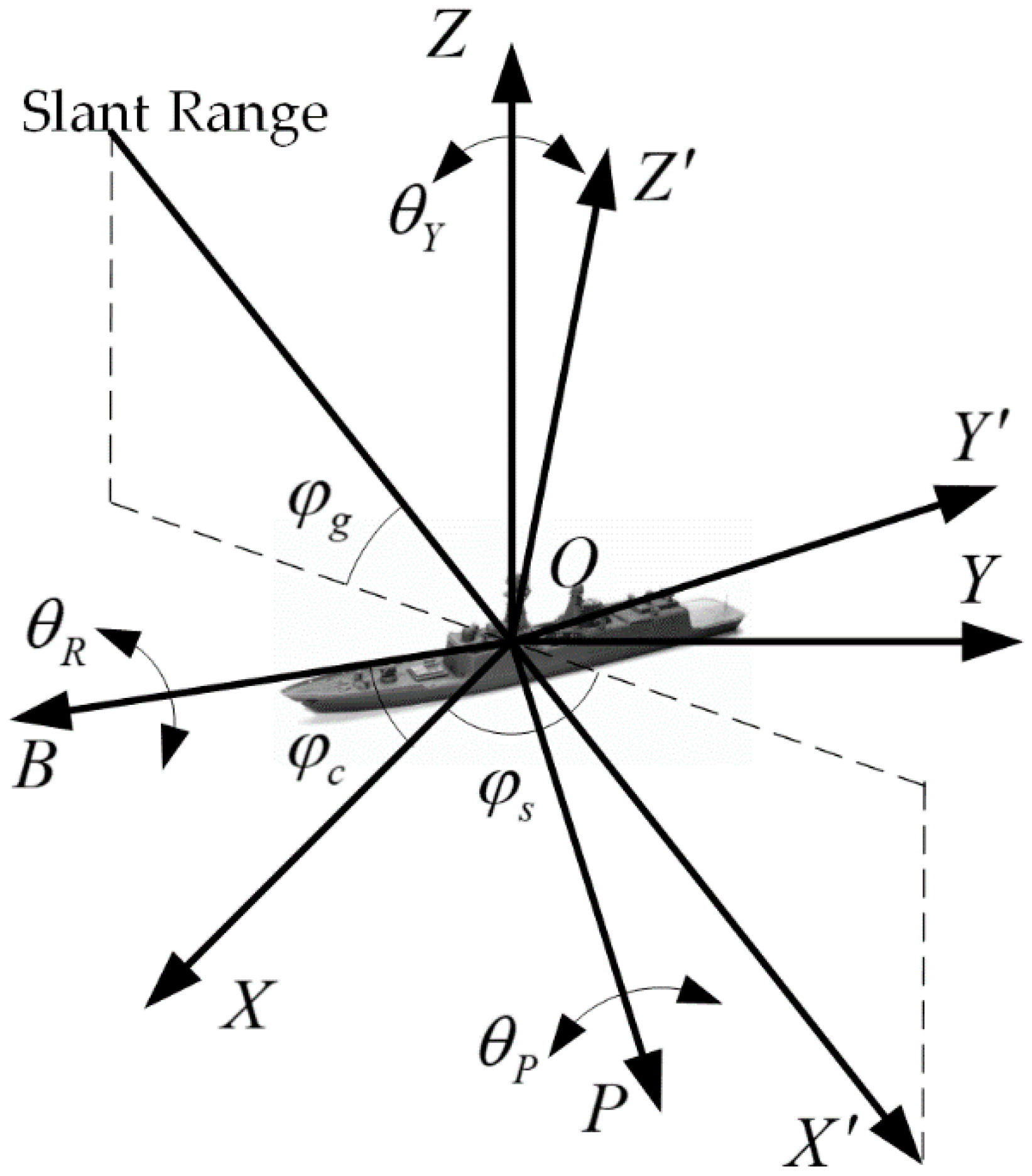
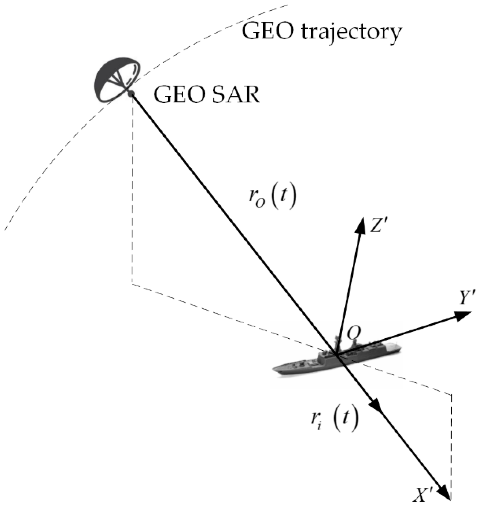
2.1. The Geometry of a Rotating Ship

The rotational effect on the slant range of a scatter point of a ship is analyzed in this section. Firstly, the rotational motion and position of a scatter point are proposed for the ship’s coordinate system. Then, the influence of rotational motion on a scatter point is transformed to the scene’s coordinate system. Finally, the influence of rotational motion is projected to the slant range of the SAR.
Figure 1 shows the general geometry of a rotating ship in GEO SAR. The ship’s fulcrum is usually made up of the gravity center O and the origin of the ship coordinate system O B P Z . The geometry of the scatter point of a ship is expressed by this coordinate system. In O B P Z , the positive B - and P -axes point to the forward direction and the port side of a ship, respectively. The Z -axis is the ship vertical axis. It is assumed that the ship only has 3D rotational motion, defined by roll, pitch, and yaw, which is measured counterclockwise from the B -, P -, and Z -axes, respectively. Based on the ship dynamics, the main forcing function driving ship rotational motions is waves at the sea surface. These waves interact with a ship’s buoyancy and hydrodynamic forces to induce oscillatory motions whose angle tends to be sinusoidal [47,48] and can be expressed as a sinusoidal function [36]:
θ r , p , y ( t ) = Θ r , p , y sin ( 2 π f r , p , y t + φ r , p , y )
where θ r , p , y represents the time-varying angles of 3D rotation such as roll, pitch, and yaw; Θ r , p , y , f r , p , y , and φ r , p , y are the amplitudes, frequencies, and initial phase of 3D rotation, respectively; and t is the slow time. Each scatter point has a coordinate at the aperture center moment (ACM). Due to the rotational motion of the ship, the coordinates change with t . To analyze the change in a scatter point’s coordinate with t , based on Euler’s rotation theorem, the transformation matrices of the roll, pitch, and yaw angles are shown as
M R = [ 1 0 0 0 cos θ r sin θ r 0 sin θ r cos θ r ]
M P = [ cos θ p 0 sin θ p 0 1 0 sin θ p 0 cos θ p ]
M Y = [ cos θ y sin θ y 0 sin θ y cos θ y 0 0 0 1 ]
where θ r , θ p , and θ y represent the roll angle θ r ( t ) , pitch angle θ p ( t ) , and yaw angle θ y ( t ) at t , respectively, whose changes follow (1).
O X Y Z is the scene coordinate system, in which the Y -axis represents the direction of the SAR platform’s velocity at the ACM. The X -axis is perpendicular to Y O Z and is determined by the right-hand rule. Then, the direction angle φ c is the angle between the B - and X -axes. The transformation matrix from O B P Z to O X Y Z can be expressed as
M 1 = [ cos φ c sin φ c 0 sin φ c cos φ c 0 0 0 1 ] .
O X Y Z is the imaging coordinate system, where the X -axis is the direction of the slant range of SAR; the Y -axis is perpendicular to the slant range and belongs to X O Y ; the Z -axis is perpendicular to X O Y and is decided by the right-hand rule. The position of the scatter point projected to the slant range and the azimuth direction at the ACM in the coordinate system O X Y Z . The transformation matrix from O X Y Z to O X Y Z is a product of the transformation matrix of the grazing angle and the angle between the X -axis and the X O Y plane, and can be written as
M 2 = [ cos φ g cos φ s cos φ g sin φ s sin φ g sin φ s cos φ s 0 sin φ g cos φ s sin φ g sin φ s cos φ g ]
where angle φ g is the grazing angle; angle φ s denotes the angle between the X -axis and the projection of the X -axis on the X O Y plane in the ACM. From (2) to (6), the coordinates for the i th scatter point in the O X Y Z coordinate system can be expressed as
[ r i ( t ) y i ( t ) z i ( t ) ] T = M 2 · M 1 · M R · M P · M Y · [ b i p i z i ] T
where [ b i p i z i ] T are the i th scatter point coordinates of a ship in the O B P Z ; y i ( t ) and z i ( t ) are the projections of the i th scatter point on the Y - and Z -axes at t , respectively; and r i ( t ) is the projection of the i th scatter point on the slant range ( X -axis) at t and can be rewritten as follows:
r i ( t ) = cos φ g cos φ c s [ b i cos θ p cos θ y + p i cos θ p sin θ y + z i sin θ p ]   + cos φ g sin φ c s [ b i ( cos θ p sin θ y + sin θ r sin θ p cos θ y ) + p i ( cos θ r sin θ y sin θ r sin θ p sin θ y ) z i sin θ r cos θ p ]   sin φ g [ b i ( sin θ p sin θ y cos θ r sin θ p cos θ y ) + p i ( sin θ r cos θ y + cos θ r sin θ p sin θ y ) + z i cos θ r cos θ p ]
where angle φ c s = φ c + φ s is the angle between the slant range and the B -axis. From (8), it can be seen that r i ( t ) is influenced by the 3D rotational motion, and it is difficult to match the rotation effect directly.

2.2. The Influence of the Rotation Effect

From (2) to (4), each degree of freedom of rotational motion can be expressed as a nested sinusoidal function:
{ sin [ Θ r , p , y sin ( 2 π f r , p , y t + φ r , p , y ) ] cos [ Θ r , p , y sin ( 2 π f r , p , y t + φ r , p , y ) ]
where mathematical symbols have the same meaning as described in (1). Based on Jacobi–Anger expansion, which is the Bessel function of the first kind, (9) can be rewritten as
{ sin [ Θ r , p , y sin ( 2 π f r , p , y t + φ r , p , y ) ] = 2 l = 0 J 2 l + 1 ( Θ r , p , y ) sin [ ( 2 l + 1 ) ( 2 π f r , p , y t + φ r , p , y ) ] cos [ Θ r , p , y sin ( 2 π f r , p , y t + φ r , p , y ) ] = J 0 ( Θ r , p , y ) + 2 l = 1 J 2 l ( Θ r , p , y ) sin [ π / 2 2 l ( 2 π f r , p , y t + φ r , p , y ) ]
where J α ( Θ r , p , y ) is the Bessel function of α order and can be expressed as
J α ( Θ r , p , y ) = ( Θ r , p , y 2 ) α k = 0 ( 1 ) k k ! ( k + α ) ! ( Θ r , p , y 2 ) 2 k .
As shown in (8), the influence of rotational motion can be expressed as the sum of the products of the sinusoidal and co-sinusoidal functions shown in (10). Fortunately, the products of the sinusoidal and co-sinusoidal functions can be rewritten as the sum of them. Therefore, (8) can be rewritten as the sum of sinusoidal functions:
r i ( t ) = n = 1 N P Θ i , n sin [ 2 π f n t + φ n ]
where f n is the frequency of the n th sinusoidal function; φ n is the initial phase of the n th sinusoidal function; n is the number of the sinusoidal function; and N p is the total number of the sinusoidal functions. From (8), it can be seen that the positions of different scatter points are not the same, i.e., b i , p i , and z i are not the same between scatter points. Therefore, the amplitudes of the sinusoidal functions of different scatter points are different, and Θ i , n represents the amplitude of the n th sinusoidal function of the i th scatter point.
The influence of rotation can be matched by (12), and the residual error of the matching result is minimal when N p = 3 in (12) (see Appendix A for the details). It can be seen that when the radar illuminates the ship, three rotational motions that trend to sinusoidal have been projected into the slant range. Although each rotation has a change in its scale after projection, there are still three sinusoidal functions projected into the slant range. Therefore, the rotation effect of a ship can be matched with the sum of three sinusoidal functions.
It is well known that the smaller the phase error is, the better the focusing effect is. Therefore, the rotational motion of a ship can be matched by gradually increasing the number of sinusoidal functions. When the total number is equal to three, the residual phase error after matching is minimal.

2.3. The Signal Model of a Ship with Rotational Motion

Figure 2 shows the geometry of a ship with rotational motion in GEO SAR. GEO SAR operates in a Geosynchronous orbit and works in the side-looking mode. The X -axis is the direction from the GEO platform to the scatter point of a ship; the Y -axis is the azimuth direction; and the Z -axis is perpendicular to X O Y plane. From (12), the slant range of a scatter point at t can be expressed as
r R i ( t ) r O ( t ) + r i ( t )
where r O ( t ) is the slant range from GEO SAR to a scatter point of a ship, which is expressed as a fourth-order Taylor series and compensates for the signal round-trip delay [25]. It can be obtained as
r O ( t ) ( r 0 + Δ r 0 ) + ( k 1 + Δ k 1 ) t + ( k 2 + Δ k 2 ) t 2 + ( k 3 + Δ k 3 ) t 3 + k 4 t 4
where r 0 , k 1 , k 2 , k 3 , and k 4 are the zero-order to fourth-order coefficients of the Taylor series, respectively; Δ r 0 , Δ k 1 , Δ k 2 and Δ k 3 are the zero-order to third-order coefficients of the Taylor series for the relative motion within the signal round-trip delay. In [25], the motion parameters of a ship with translational motion can be estimated in GEO SAR. Therefore, we assume that the translational motion has been compensated for and the coefficients of r O ( t ) are known from the motion of the GEO platform in this paper.
As shown in (12) and Section 2.2, the rotation effect of a ship can be matched by the sum of three sinusoidal functions, and (13) can be rewritten as
r R i ( t ) r O ( t ) + r i ( t ) = r O ( t ) + n = 1 3 Θ i , n sin [ 2 π f n t + φ n ] .
The influence of rotational motion on the range cell migration is analyzed in Appendix B. From the analysis result and the optimal resolution of GEO SAR ( ρ r _ b e s t = 5 m ), it is shown that the rotational motion is less than half of the optimal resolution, and its influence does not cause range cell migration in GEO SAR.
So, after the range compression, the echo signal model can be given as
s r m ( t , τ ) A r m sin c ( B s ( τ 2 r O ( t ) c ) ) exp ( j 4 π r R i ( t ) λ )
where B s = γ T p , T p , and γ are the pulse bandwidth, the pulse duration of the transmitting signal, and the frequency modulation rate of the linear frequency modulated (LFM) signal, respectively; A r m = T p B s A r is the amplitude after the range compression and A r is the amplitude before the range compression.

3. The Rotational Ship Imaging Method Based on the Matching of Multiple Sinusoidal Functions

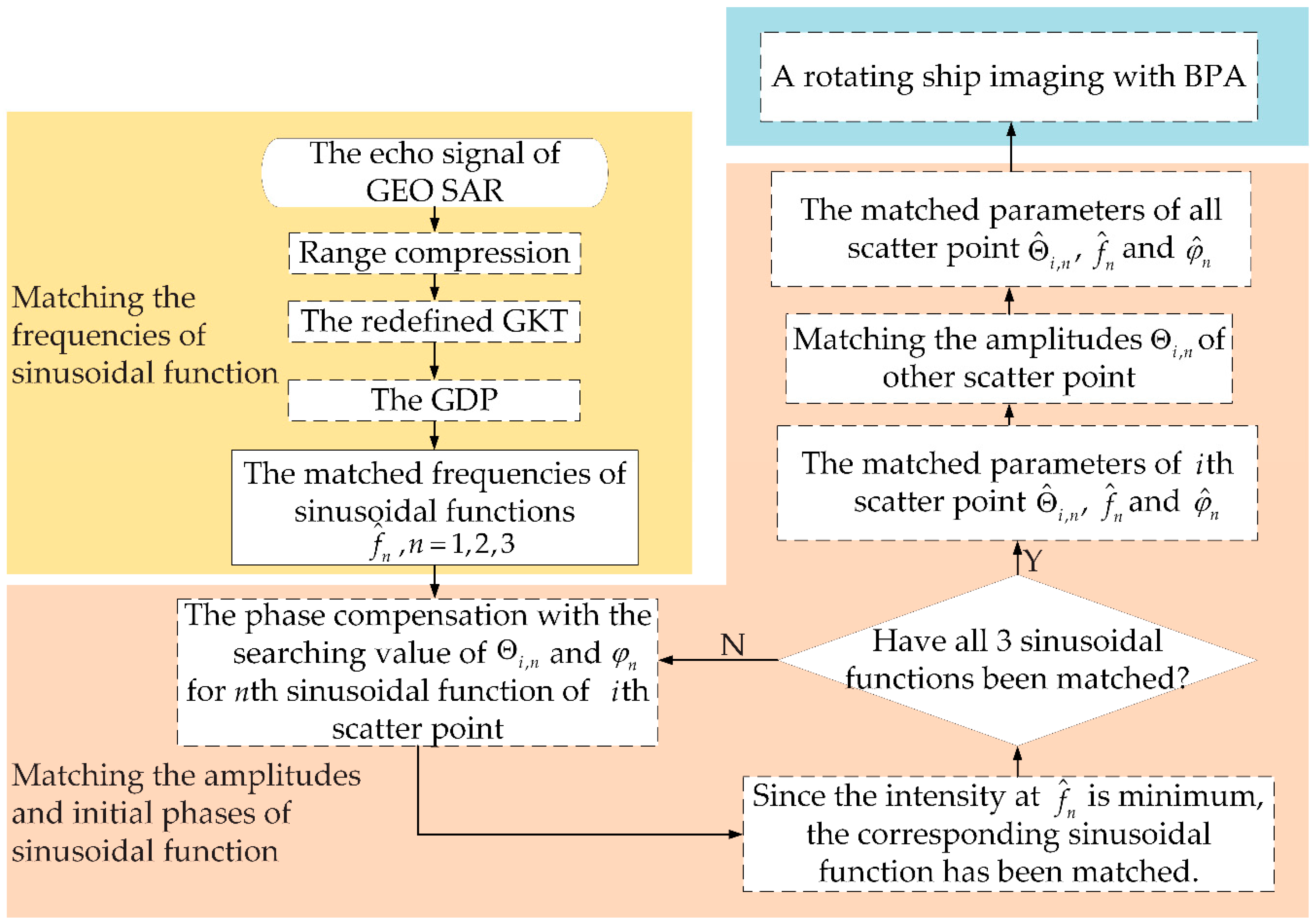
3.1. The Rotation Effect Matching and Ship Imaging Procedure

As shown in Section 2, the influence of rotational motion can be matched by the sum of three sinusoidal functions. The multiple sinusoidal function matching-based rotational ship imaging method is summarized in Figure 3. It comprises the following three steps:
Step 1: Match the frequencies of sinusoidal function
After range compression, the echo signal is as shown in (16). Firstly, the range migration caused by the motion of the GEO platform is corrected with the modified GKT (see Section 3.2). Then, the phase caused by the platform motion is compensated for with the GDP. Because the rotational motion can be matched by the sum of three sinusoidal functions, the signal is focused at the frequencies of three sinusoidal functions in the Range-Doppler (RD) domain, and the frequencies f ^ n , n = 1 , 2 , 3 can be matched by the position where the signal has focused.
Step 2: Match the amplitudes and initial phases of sinusoidal function
Although the frequencies of sinusoidal function f ^ n are matched in Step 1, the amplitudes Θ i , n and initial phases φ n still need to be matched. Because the intensities of signal at f ^ n are different, the sinusoidal functions with the maximal and minimal intensity are named as the 1st and 3rd sinusoidal functions, respectively. The rest of sinusoidal function is named as the 2nd sinusoidal function. Firstly, Θ i , 1 and φ 1 of the 1st sinusoidal function, are searched, and the searching values are used to compensate for the influence of the 1st sinusoidal function. For different searching values, the intensities of compensation results at f ^ 1 are different. Since the intensity at f ^ 1 is minimal, the influence of the 1st sinusoidal function is matched, and the searching values of the amplitude and initial phase are the matched values of Θ ^ i , 1 and φ ^ 1 , respectively. Then, the same approach is taken to compensate for the influences of the 2nd and 3rd sinusoidal functions. Since the influences of all three sinusoidal functions are compensated for, the frequencies f ^ n , initial phases φ ^ n , and amplitudes Θ ^ i , n of the i th scatter point are matched.
However, because different scatter points have the same frequencies and phases but different sinusoidal function amplitudes Θ i , n , the amplitudes of other scatter points need to be matched. Similarly, to match the sinusoidal functions of the i th scatter point, the Θ i , 1 of the 1st sinusoidal function is searched in the range cell where the scatter point is, and the searching value is used to compensate for the influence of the 1st sinusoidal function. With the different searching value, the intensities of compensation results at f ^ 1 are different. Since the intensity at f ^ 1 is minimal, the influence of the 1st sinusoidal function is compensated for, and the searching value of the amplitude is the matched value of Θ ^ i , 1 . Then, the Θ i , 2 of the 2nd sinusoidal function is searched in the range cell. Since the intensity at f ^ 2 is minimal, the searching value of the amplitude is the matched with the value of Θ ^ i , 2 . Then, Θ i , 3 was searched in the same way. Since the influences of all three sinusoidal functions are compensated for, the amplitude Θ ^ i , n of the scatter point is matched. Furthermore, when the amplitudes of all scatter points are matched, the influence of rotational motion matching is realized.
Note that scatter points’ focusing in Steps 1 and 2 are in the RD domain and to match the parameters of sinusoidal functions. To realize the imaging of a ship, an imaging algorithm needs to focus each scatter point with the matched parameters in a 2D time domain.
Step 3: Ship imaging with the BPA
In Steps 1 and 2, the f n , φ n , and Θ i , n of each scatter point of a ship are matched. Based on the matched values, a ship can be imaged by BPA.

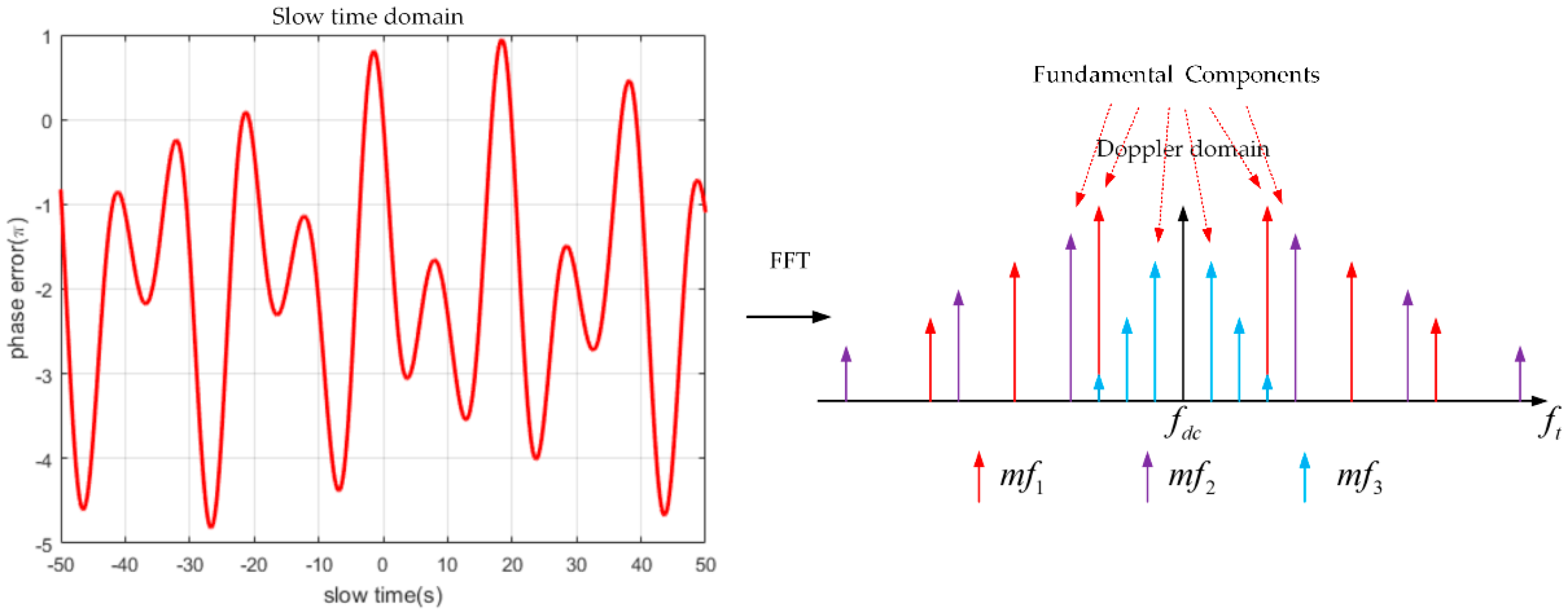
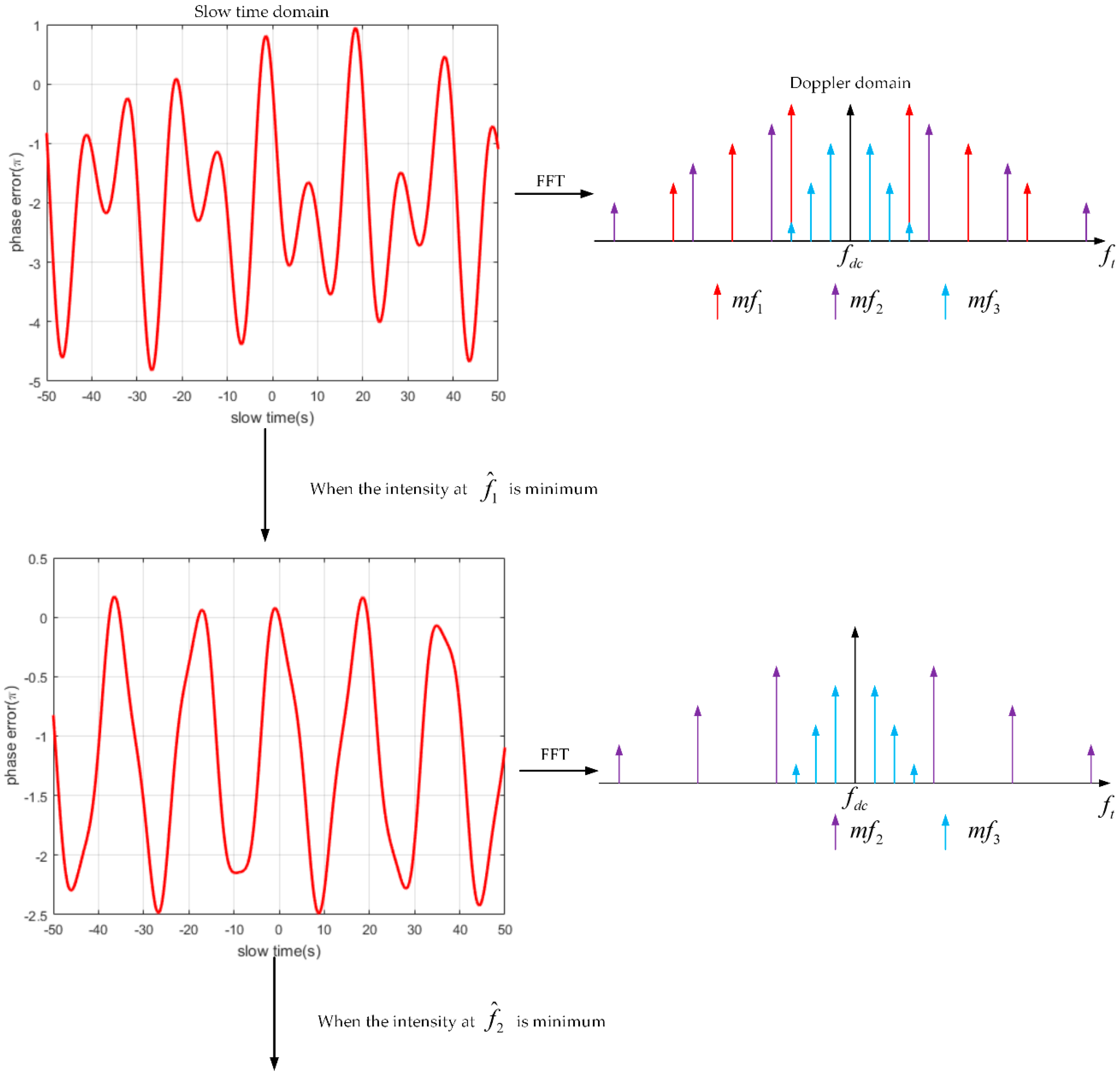
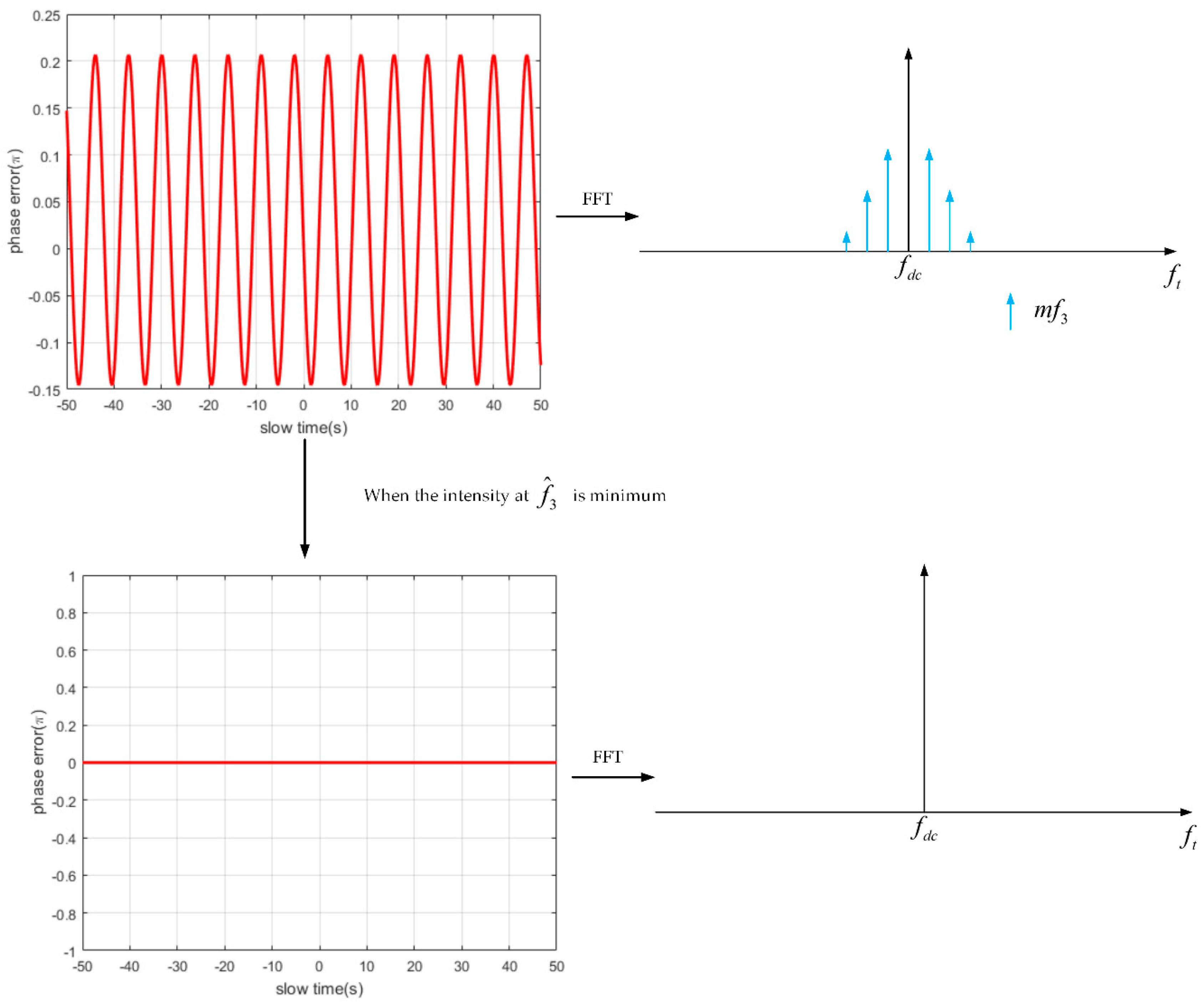
3.2. Matching the Frequencies of Sinusoidal Function

The Keystone Transform (KT) is a common method to eliminate the effects of linear range migration [49]. Furthermore, the Generalized KT (GKT) has been proposed to eliminate high-order range migration [46]. In this Section, the GKT is modified to correct for the range migration caused by the motion of the GEO platform. The GDP is used to compensate for the phase caused by the platform’s motion, and the frequencies of sinusoidal function can be matched in the RD domain. After transforming (16) into the slow time-range frequency domain, the signal can be expressed as
S r m ( t , f τ ) = A 1 r e c t ( f τ / B s ) exp ( j 4 π ( f τ + f c ) r R i ( t ) c )
where f τ is the range frequency corresponding to the fast time τ ; f c is the carrier frequency; and A 1 is the amplitude of the signal in the slow time-range frequency domain. Substituting (14) and (15) into (17) yields
S r m ( t , f τ ) = A 2 exp ( j 4 π ( f τ + f c ) c ( r 0 + Δ r 0 ) )   · exp ( j 4 π ( f τ + f c ) c ( k 1 + Δ k 1 ) t )   · exp ( j 4 π ( f τ + f c ) c ( k 2 + Δ k 2 ) t 2 )   · exp ( j 4 π ( f τ + f c ) c ( k 3 + Δ k 3 ) t 3 )   · exp ( j 4 π ( f τ + f c ) c k 4 t 4 )   · exp ( j 4 π ( f τ + f c ) c r i ( t ) )
where A 2 = A 1 r e c t ( f τ / B s ) . To correct the fourth-order range migration caused by k 4 , the fourth-order KT is performed along the slow time domain and the scaling formula can be written as
t = [ f c / ( f τ + f c ) ] 1 4 t 4 .
Substituting (19) into (18) yields
S r m ( t 4 , f τ ) = A 2 exp ( j 4 π λ ( f τ + f c ) f c ( r 0 + Δ r 0 ) )   · exp ( j 4 π λ ( ( f τ + f c ) f c ) 3 / 4 ( k 1 + Δ k 1 ) t 4 )   · exp ( j 4 π λ ( ( f τ + f c ) f c ) 1 / 2 ( k 2 + Δ k 2 ) t 4 2 )   · exp ( j 4 π λ ( ( f τ + f c ) f c ) 1 / 4 ( k 3 + Δ k 3 ) t 4 3 )   · exp ( j 4 π λ k 4 t 4 4 )   · exp ( j 4 π λ ( f τ + f c ) f c r i ( t 4 ) )
where λ = c / f c . Correspondingly, the fourth-order phase can be compensated by following function
M 4 ( t 4 ) = exp ( j 4 π λ k 4 t 4 4 ) .
By multiplying (20) with (21), we have
S r m ( t 4 , f τ ) = A 2 exp ( j 4 π λ ( f τ + f c ) f c ( r 0 + Δ r 0 ) )   · exp ( j 4 π λ ( ( f τ + f c ) f c ) 3 / 4 ( k 1 + Δ k 1 ) t 4 )   · exp ( j 4 π λ ( ( f τ + f c ) f c ) 1 / 2 ( k 2 + Δ k 2 ) t 4 2 )   · exp ( j 4 π λ ( ( f τ + f c ) f c ) 1 / 4 ( k 3 + Δ k 3 ) t 4 3 )   · exp ( j 4 π λ ( f τ + f c ) f c r i ( t 4 ) )
Similarly, the third-order range migration and phase caused by ( k 3 + Δ k 3 ) are compensated by the third-order KT and phase compensation, respectively. The third-order scaling formula for KT is given in (23); the third-order phase compensation function is given in (24):
t 4 = [ f c / ( f τ + f c ) ] 1 12 t 3
M 3 ( t 3 ) = exp ( j 4 π λ ( k 3 + Δ k 3 ) t 3 3 ) .
After the third-order KT and phase compensation, (22) can be rewritten as
S r m ( t 3 , f τ ) = A 2 exp ( j 4 π λ ( f τ + f c ) f c ( r 0 + Δ r 0 ) )   · exp ( j 4 π λ ( ( f τ + f c ) f c ) 2 / 3 ( k 1 + Δ k 1 ) t 3 )   · exp ( j 4 π λ ( ( f τ + f c ) f c ) 1 / 3 ( k 2 + Δ k 2 ) t 3 2 )   · exp ( j 4 π λ ( f τ + f c ) f c r i ( t 3 ) )
Then, to compensate for the range migration and phase caused by ( k 2 + Δ k 2 ) , the second-order scaling formula for KT and phase compensation function are expressed as (26) and (27), respectively:
t 3 = [ f c / ( f τ + f c ) ] 1 6 t 2
M 2 ( t 2 ) = exp ( j 4 π λ ( k 2 + Δ k 2 ) t 2 2 ) .
Because the motion parameters of GEO SAR are already known, the range migration and phase caused by ( k 1 + Δ k 1 ) can be compensated for. The first-order scaling formula for KT and the phase compensation function are expressed as (28) and (29), respectively:
t 2 = [ f c / ( f τ + f c ) ] 1 2 t 1
M 1 ( t 1 ) = exp ( j 4 π λ ( k 1 + Δ k 1 ) t 1 ) .
After second- and first-order range migration and phase are compensated for, (25) can be rewritten as
S r m ( t 1 , f τ ) = A 2 exp ( j 4 π λ ( f τ + f c ) f c ( r 0 + Δ r 0 ) ) exp ( j 4 π λ ( f τ + f c ) f c r i ( t 1 ) ) .
After performing an inverse fast Fourier transform (IFFT) along the range frequency domain, (30) can be expressed as
s RCMC ( t 1 , τ ) A 4 exp ( j 4 π λ r i ( t 1 ) )
where A 4 = A 3 sin c ( B s ( τ 2 ( r 0 + Δ r 0 ) / c ) ) exp ( j 4 π ( r 0 + Δ r 0 ) / λ ) ; A 3 is the amplitude of the signal after performing an IFFT. From (12), the influence of rotational motion can be matched by the sum of three sinusoidal functions, and (31) can be rewritten as
s ( t 1 , τ ) A 4 exp ( j 4 π λ n = 1 3 Θ i , n sin [ 2 π f n t 1 + φ n ] ) .
Using (18) to (32), the first- to fourth-order range migration and phase are compensated for by KT and the phase compensation function, respectively. Each order of KT is collectively referred to as the generalized KT (GKT). Correspondingly, the first- to fourth-order phases need to be compensated for by the phase compensation function, which is similar to the Dechirp process (DP). Therefore, each order of phase compensation is collectively referred to as the generalized DP (GDP). Furthermore, each sinusoidal function can be expressed as a Bessel series [41].
exp [ j 4 π λ Θ sin ( 2 π f t + φ ) ] = m = J m ( 4 π λ Θ ) exp [ j m ( 2 π f t + φ ) ]
where m is the number of harmonics, and α and β represent any amplitude and phase, respectively. From (33), (32) can be rewritten as
s ( t 1 , τ ) A 4 n = 1 3 exp ( j 4 π λ Θ i , n sin [ 2 π f n t 1 + φ n ] )   = A 4 n = 1 3 m = J m ( 4 π λ Θ i , n ) exp [ j m ( 2 π f n t 1 + φ n ) ]
Then, after transforming (34) into the RD domain, the signal will be focused at the frequency m f n [50,51,52]. A schematic diagram is shown in Figure 4. After GKT and GDP, the signal can be expressed as shown in (34) and is focused at the frequencies of sinusoidal function and the integral multiples of frequencies in the RD domain. Furthermore, from the Bessel function, the signal at ± f n is a fundamental component, and its intensity is greater. Meanwhile, the signal at m f n , m = ± 2 , ± 3 , are harmonic components, and their intensities are weak. Therefore, because the harmonic components are weak, the frequencies of sinusoidal function ± f n are easy to distinguish and can be matched by the position where the fundamental component of signal is focused, and the matched values of frequency are f ^ n , n = 1 , 2 , 3 .

3.3. Matching the Amplitudes and Initial Phases of Sinusoidal Function

From Section 3.2, after GKT and GDP, the signal can be focused on the frequencies of sinusoidal function, and the frequencies can be matched. However, from (15), the amplitudes Θ i , n and initial phases φ n of sinusoidal function also need to be matched.
Obviously, each compensation of the sinusoidal function can make the signal better focused at the Doppler center frequency f d c . A schematic diagram is shown in Figure 5.
Based on (34), searching parameters and phase compensation with searching values for each sinusoidal function in a range cell are shown in Figure 5. Firstly, the 1st sinusoidal function of (32) is compensated for by searching Θ i , 1 and φ 1 . When the intensity at f ^ 1 is minimal, the influence of the 1st sinusoidal function is compensated for and the searching values of the amplitude and initial phase are the matched values of Θ ^ i , 1 and φ ^ 1 , respectively. Then, the 2nd and 3rd sinusoidal functions are compensated for with the same method. The compensation function for the influence of the sinusoidal function can be expressed as
M s , n ( t 1 ) = exp ( j 4 π λ Θ ˜ i , n sin [ 2 π f ^ n t 1 + φ ˜ n ] ) , n = 1 , 2 , 3
where Θ ˜ i , n and φ ˜ n are the searching values of the amplitude and the initial phase of the n th sinusoidal function, respectively. In the process of compensating for each sinusoidal function separately, the intensity at f d c in the RD domain gradually increases. According to (32), when all of the sinusoidal functions are compensated for, the signal can be expressed as
s ( t 1 , τ ) A 3 sin c ( B s ( τ 2 ( r 0 + Δ r 0 ) / c ) ) exp ( j 4 π ( r 0 + Δ r 0 ) / λ ) .
Transforming (36) into the RD domain yields
S ( f t , τ ) A 5 sin c ( B s ( τ 2 ( r 0 + Δ r 0 ) / c ) ) exp ( j 4 π ( r 0 + Δ r 0 ) / λ )   · sin c ( T C P I ( f t f d c ) )
where T C P I is the CPI and f d c is the Doppler center frequency. As shown by (37), after all three sinusoidal functions have been compensated for, the signal can be completely focused at f d c , i.e., the intensity at f d c is maximal.
Correspondingly, the f ^ n , φ ^ n , and Θ ^ i , n of all three sinusoidal functions for the i th scatter point are matched. However, as shown in Section 2.2, because the amplitude of the sinusoidal function at different scatter points of a ship is not the same, the amplitudes of other scatter point need to be matched.
Similarly, Θ i , 1 is searched and the 1st sinusoidal function of (32) is compensated for by searching for values in a range cell including the scatter point to be matched. When the intensity at f ^ 1 is minimal, the searching value of the amplitude is the matched value of Θ ^ i , 1 . Then, Θ i , 2 and Θ i , 3 are matched with the same method. Furthermore, when the amplitudes of all scatter points are matched, the matched values of Θ i , n , f n , and φ n for all scatter points can be obtained. When the parameters of rotational motion are non-constant in the whole CPI, the rotational motion cannot be matched accurately. Fortunately, the rotation should be constant in a sub-aperture, and the proposed method can be used in a sub-aperture.

3.4. Ship Imaging with BPA and Matched Parameters of Sinusoidal Functions

As mentioned above, the influence of rotational motion can be matched by the sum of three sinusoidal functions, and a matching method for the parameters of sinusoidal functions has been proposed. Although the influence of rotational motion can be matched, different from static targets, each scatter point of a ship moves differently due to the 3D rotational motion of the ship. Most of the existing imaging algorithms, such as (Range Doppler) RD, (Chirp Scaling) CS, and SPECtral ANalysis (SPECAN), cannot be used to image scatter points with different motions.
After range compression, the echo signal is distributed in different range cells. In the BPA, the signal is integrated along its slant range, and the integration result is the image of the target. The BPA calculates the range migration of different scatter points separately and can be used as the imaging method of a ship. As shown in (16), the imaging for the i th scatter point can be expressed as
I ( m i , n i ) = T C P I / 2 T C P I / 2 s r m ( t , 2 r ^ R i ( t ) c ) exp ( j 4 π r ^ R i ( t ) λ ) d t
where s r m is the echo model after the range compression and expressed as (16); r ^ R i ( t ) is the matched slant range of the i th scatter point and can be written as
r ^ R i ( t ) ( r 0 + Δ r 0 ) + ( k 1 + Δ k 1 ) t + ( k 2 + Δ k 2 ) t 2 + ( k 3 + Δ k 3 ) t 3 + k 4 t 4   + n = 1 3 Θ ^ i , n sin [ 2 π f ^ n t + φ ^ n ]

4. Simulation Results and Discussion

In this Section, numerical experiments are carried out to verify the effectiveness of the proposed multiple sinusoidal function matching-based rotational ship imaging method in GEO SAR. In Section 4.1, the matching method for the frequencies of sinusoidal functions, which was proposed in Section 3.2, is verified. Then, in Section 4.2, the matching method for the amplitudes and initial phases of sinusoidal functions, which was proposed in Section 3.3, is verified. Then, in Section 4.3, based on the matched values in Section 4.1 and Section 4.2, the BPA for a rotating target, which was proposed in Section 3.4, is verified. Finally, in Section 4.4, the 2D raw echoes of a rotating ship are generated in the apogee of GEO SAR to verify the imaging method proposed in Section 3.1. The system parameters of GEO SAR used for the simulation are listed in Table 1; the parameters of rotational motion for the simulation are listed in Table 2.

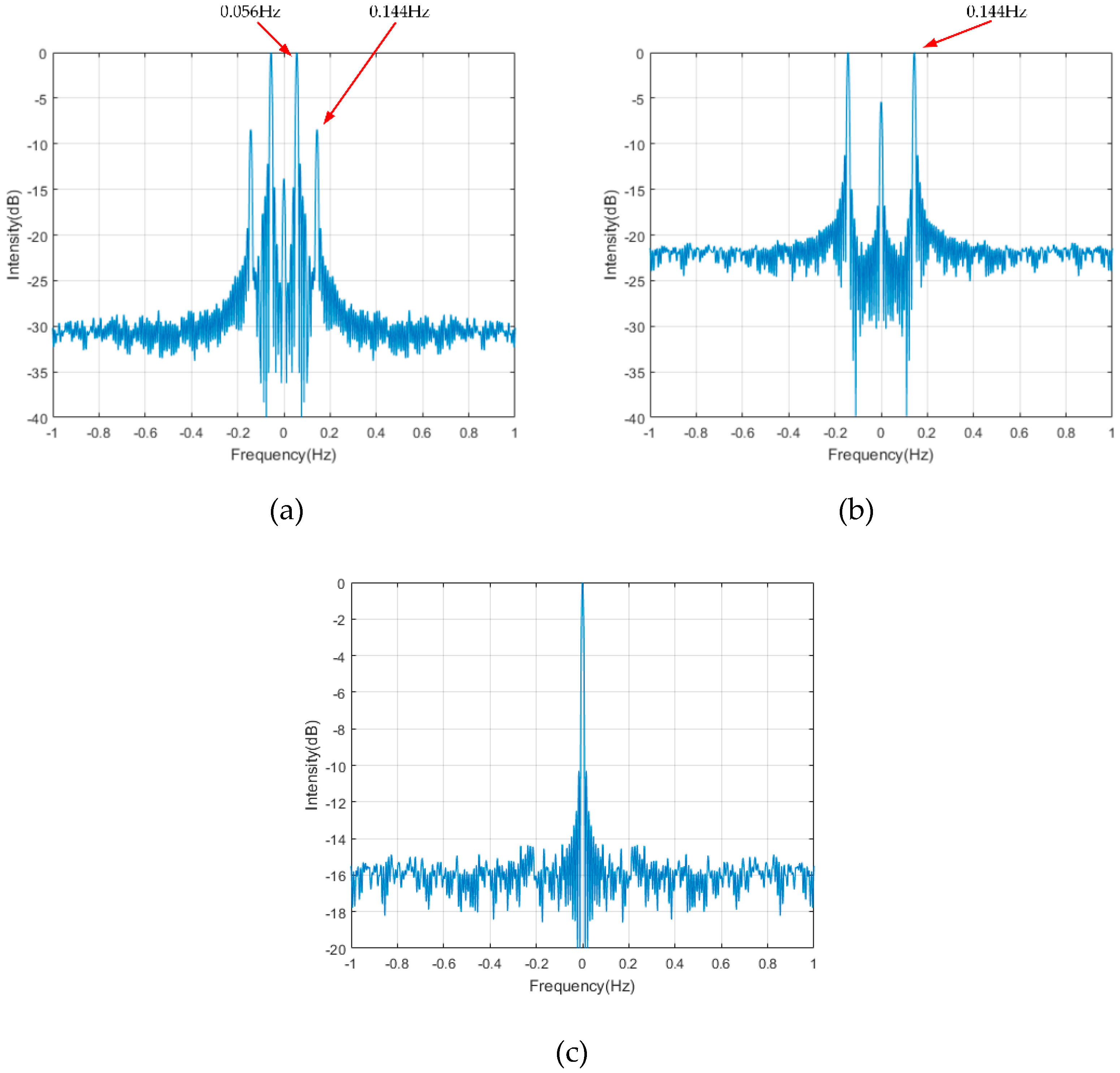
4.1. Simulation Results for Matching the Frequencies of Sinusoidal Function

Based on (8), we generated the echoes of a ship target represented by a scatter point [ b i p i z i ] = [ 100 100 0 ] ( m ) with rotational motion into the background raw data of GEO SAR. The parameters of the rotational motion are shown as Table 2. Furthermore, the imaging of a ship just by existing BPA, which can be obtained by (38) and (39) without the matched results for rotational motion, is shown in Figure 6. From Figure 6, although the range migration and phase caused by the GEO platform has been compensated, a ship cannot be focused on without rotational motion compensation, and the signal energy has spread in a range cell.
After range compression, the echo signal is as shown in Figure 7a. Due to the motion of GEO SAR, the echo signal is distributed across several range cells. Based on the method proposed in Section 3.2, after GKT and GDP, the range migration and the phase caused by the motion of the GEO platform are compensated, and the simulation results are as shown in Figure 7b.
As shown by (34), after the GKT and GDP, the rotational motion can be matched by the sum of three sinusoidal functions, and the signal focuses at the frequencies of three sinusoidal functions in the RD domain [52]. Therefore, an Fast Fourier transform (FFT) that was performed along the azimuth direction and the Doppler profile are shown in Figure 8. The signal is focused at the frequencies of three sinusoidal functions, and the matched values of three frequencies f ^ n are 0.100   Hz , 0.056   Hz , and 0.144   Hz .

4.2. Simulation Results for Matching the Amplitudes and Initial Phases of the Sinusoidal Function

In Section 4.1, the matched values of three frequencies of the sinusoidal function were obtained. As shown in Figure 8, because the intensity at a frequency of 0.100   Hz is maximal, the amplitude and the initial phase of the sinusoidal function with a frequency of 0.100   Hz were matched first. The phase compensation was performed using (35). When the intensity at f ^ 1 = 0.100   Hz was minimal (shown in Figure 9a), the matched values of the amplitude and the initial phase were equal to Θ ^ i , 1 = 0.094 and φ ^ 1 = 2.618 , respectively. Then, similarly, the amplitude and the initial phase of the sinusoidal function were matched with a frequency of f ^ 2 = 0.056   Hz . The intensity at f ^ 2 = 0.056   Hz was minimal, and the simulation results are shown in Figure 9b. Finally, the 3rd sinusoidal function was matched with a frequency of f ^ 3 = 0.144   Hz , and the simulation results are shown in Figure 9c. The matched values of the amplitude and the initial phase for each sinusoidal function are shown in Table 3.
From Figure 9, when all of three sinusoidal functions have been matched, the intensity at f d c is largest.

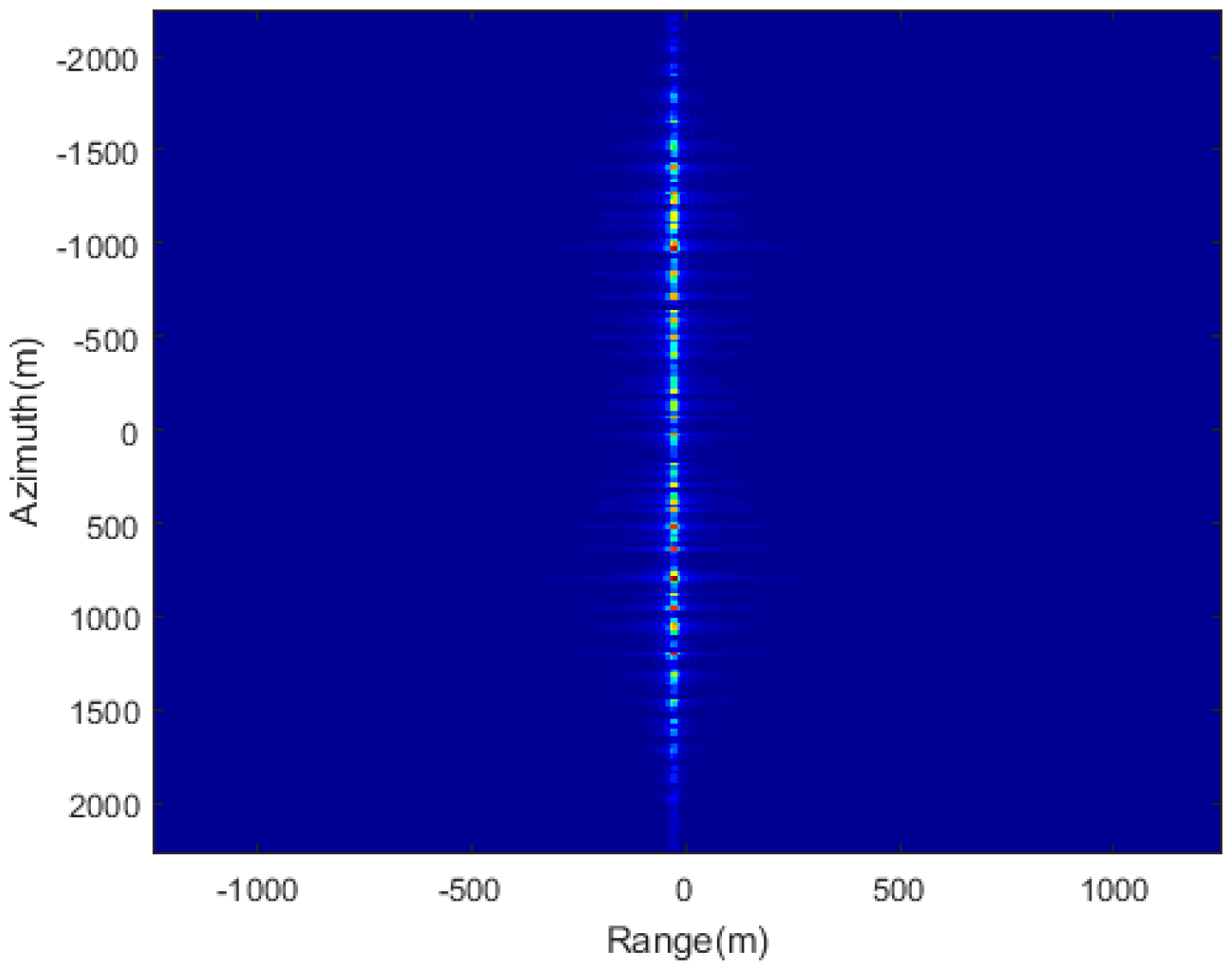
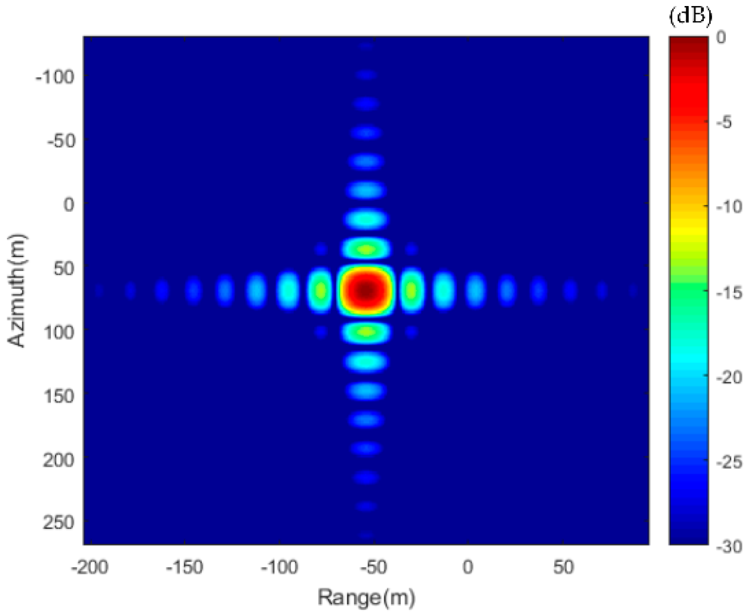
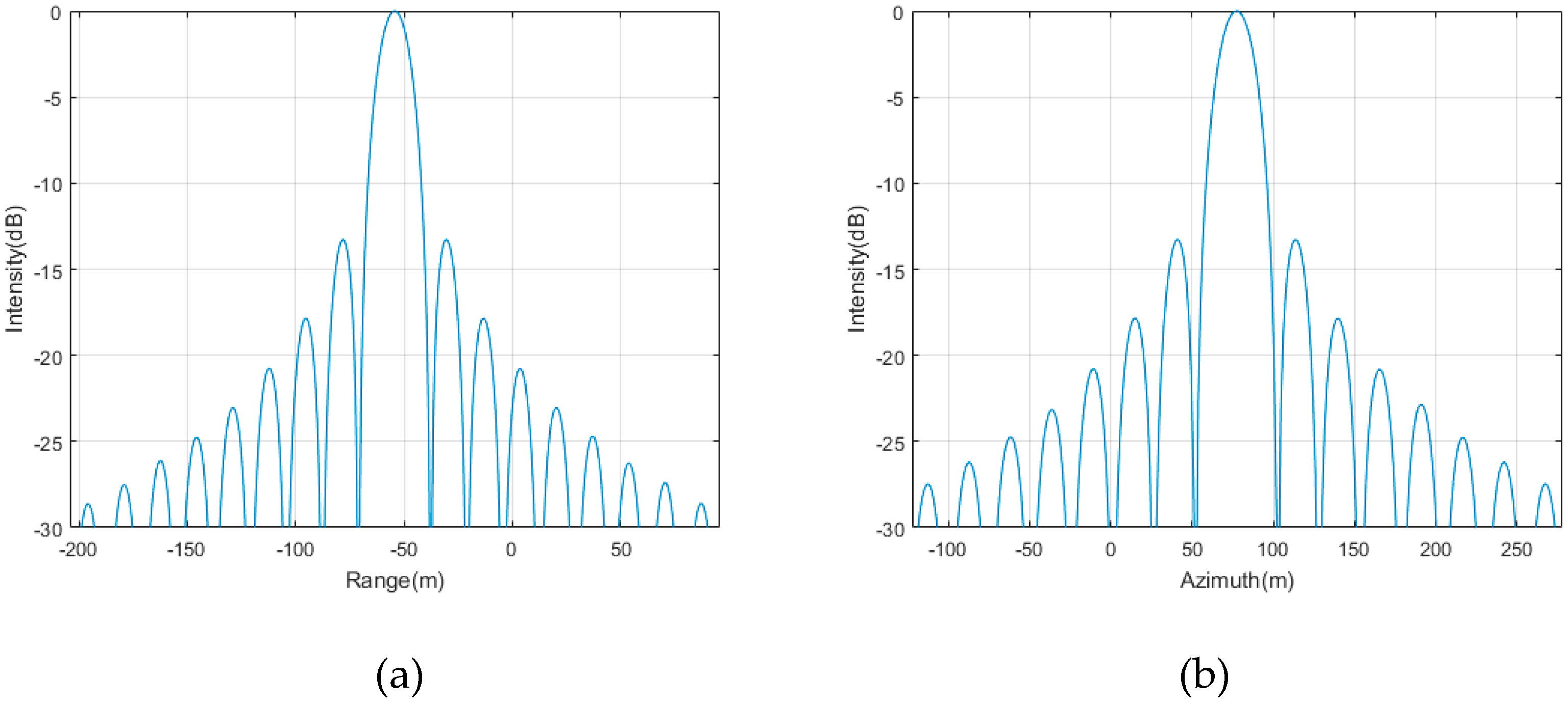
4.3. The Simulation Results for the BPA

In Section 4.1 and Section 4.2, the parameters of the sinusoidal functions were matched. In this section, the images with the matched values (listed in Table 3) are obtained. The imaging of a target was simulated using (38), and the simulation results are shown in Figure 10. The range and azimuth profile of the imaging result are shown in Figure 11. The Peak Side Lobe Ratio (PSLR) of the target in the range and azimuth directions was –13.27 and –13.25 dB, respectively. The simulation results show that before matching the rotational motion, the target cannot be focused (shown as Figure 6). After matching the influence of rotation, as described in in Section 4.1 and Section 4.2, the target can be completely focused with the proposed imaging method.

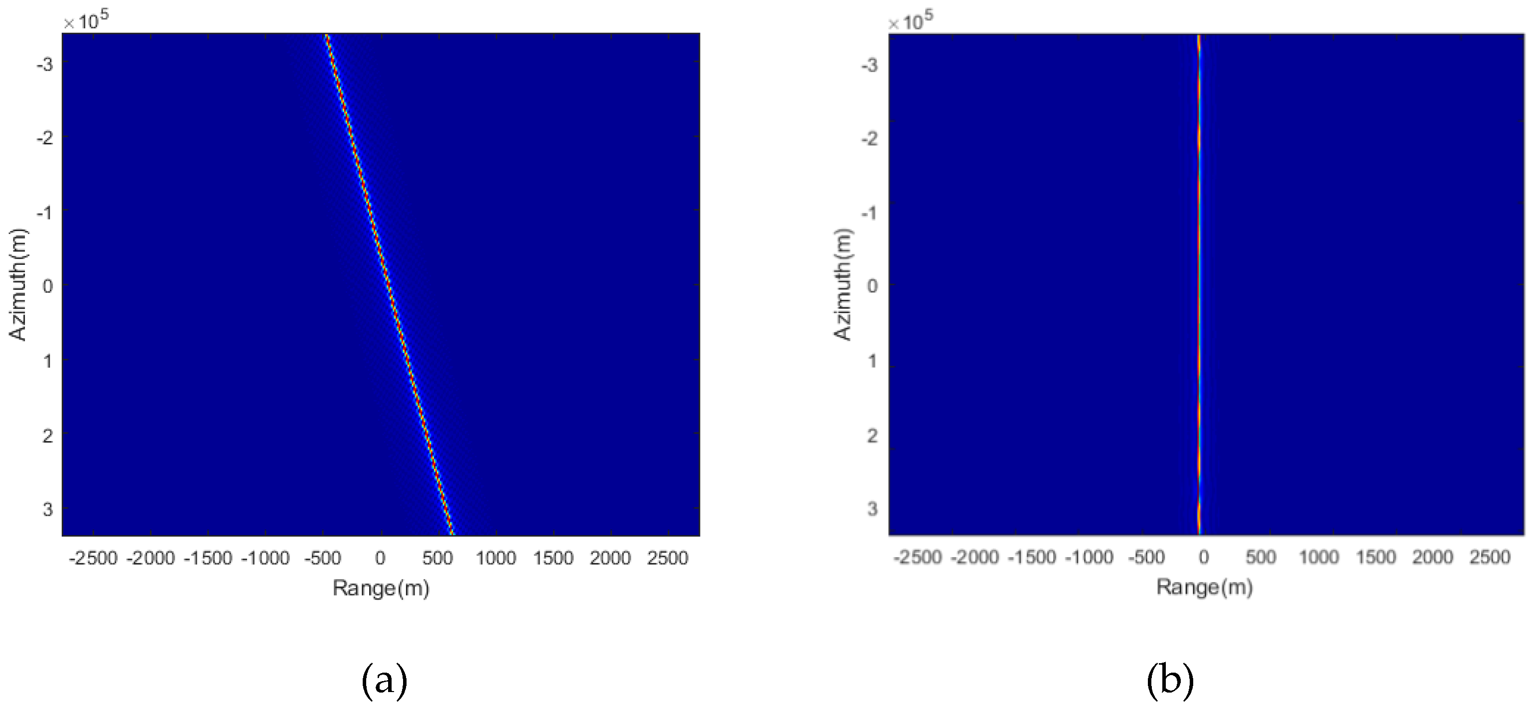
4.4. The Simulation Results for the Proposed Rotating Ship Imaging Method

In this section, the effectiveness of the imaging methods proposed in Section 3.1 is verified. A ship is represented by five scatter points and is added to an echo signal of GEO SAR. The coordinates of five scatter points are listed in Table 4; the parameters of rotation are the same as those shown in Table 2. Due to the influence of rotation, scatter points A to D cannot be focused, which is shown in Figure 12a. scatter point E is located at the gravity center of a ship, where the rotational motion does not influence the focus.
Based on the method proposed in Section 3.2 and Section 3.3, the matched values of sinusoidal functions are as shown in Table 5. Based on Section 3.4, the imaging results of a rotating ship are shown in Figure 12b. The simulation results show that without matching the rotation effect, the ship cannot be focused. Correspondingly, a ship can be completely focused when the method proposed in Section 3.1 is used. In this paper, each scatter point needs to match with three amplitudes of the sinusoidal functions and the amplitudes are matched one by one. In numerical experiments, the search accuracy of each amplitude for a scatter point is 1/1000 rad and the search scope is [ π / 2 π / 2 ] rad—it takes several minutes for each scatter point to be matched.

5. Conclusions

Compared with other SAR platforms, the CPI of GEO SAR is very long (in the order of hundreds of seconds). The existing methods, which match the influence of rotational motion within seconds of the CPI via the high-order Taylor series, are obviously inapplicable.
To solve the problems for rotating ship imaging with a long CPI of GEO SAR, a novel ship imaging method using multiple sinusoidal functions to match the rotation effect was proposed. First, the analysis results show that the influence of the rotation effect can be matched using the sum of three sinusoidal functions, and the signal model of a rotating ship in GEO SAR was obtained. Then, the multiple sinusoidal function matching-based ship imaging method was proposed. Its procedure includes (1) the modification of the GKT to correct the range migration caused by the motion of the GEO platform. After the phase caused by the platform motion is compensated for by the GDP, the signal focuses at the frequencies of sinusoidal functions in the RD domain, and the frequencies can be matched. (2) The amplitudes and initial phases of sinusoidal functions are matched via phase compensation with parameter searching. (3) Based on the matched parameters of sinusoidal functions, the rotating ship is imaged via BPA.
Finally, numerical experiments were conducted to demonstrate the effectiveness of the proposed method in GEO SAR with an orbit inclination of 53°. The simulation results show that the proposed method can realize rotating ship imaging with a range and azimuth PSLR of about −13.27 and −13.25 dB, respectively. In general, ships have a higher radar cross-section against the surrounding sea background because of metallic materials and corner reflection structures [53]. Sometimes, the clutter from the sea surface cannot be ignored, and it extends the Doppler bandwidth and influences the proposed method. A realization of the proposed method with clutter from the sea surface will be considered in future work.

Author Contributions

Y.Z. and X.D. conceived and designed the method; W.X. guided the students to complete the research; Z.L., M.X. and C.C. performed the simulation and experiment; Y.Z. and X.D. wrote the paper. All authors have read and agreed to the published version of the manuscript.

Funding

This research was funded in part by the National Natural Science Foundation of China under Grant Nos. 31727901, 61960206009, 61971039, 61971037, National Ten-thousand Talents Program ‘Young top talent’ (Grant No. W03070007), and the Young Elite Scientists Sponsorship Program by CAST (2017QNRC001).

Acknowledgments

The authors would like to thank all reviewers and editors for their comments on this paper.

Conflicts of Interest

The authors declare no conflict of interest.

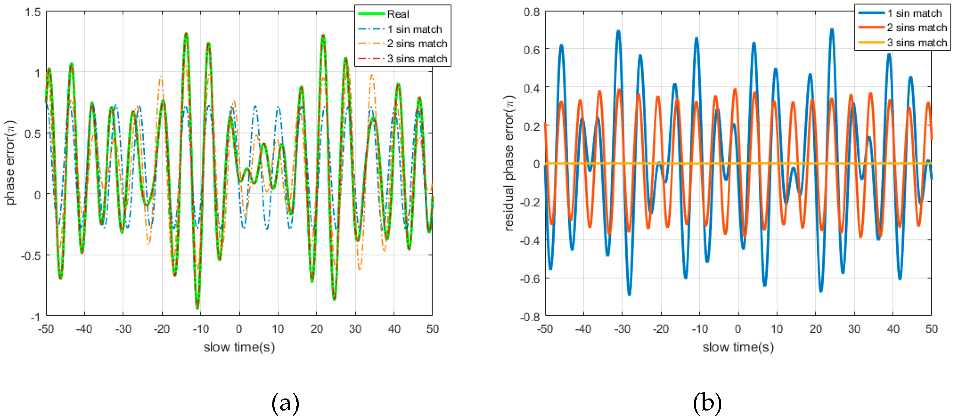
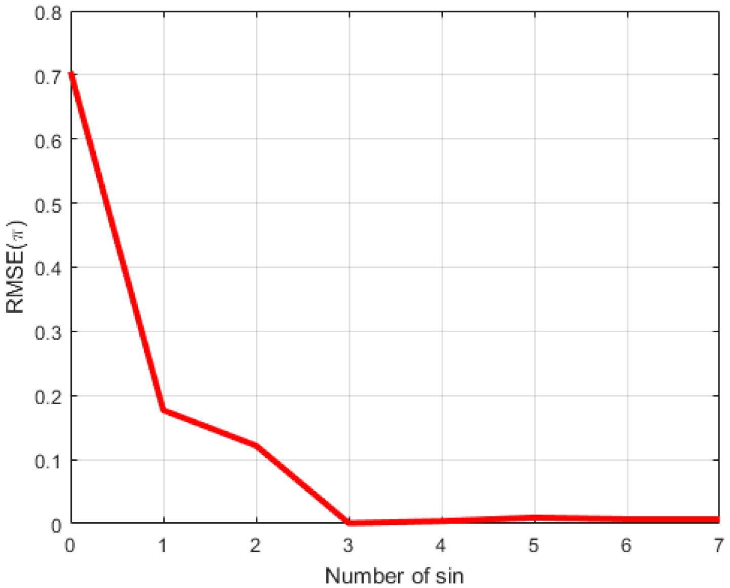
Appendix A. The Effectiveness of (12) and the Residual Error with Different Numbers of Sinusoidal Functions

To verify the effectiveness of (12), the rotational effect of the ship in (8) was determined by the sum of the sinusoidal functions via the nonlinear least squares method. The rotational motion parameters are listed in Table A1, where the amplitudes and frequencies of the rotational motion are given based on the typical values of a ship [47]. The sum of sinusoidal functions 1–3 shown in (12) is used to match the rotational motion of the scatter point [ b i p i z i ] = [ 100 50 10 ] ( m ) in the ship’s coordinate system. The matched results of the phase error caused by rotation within 100 s of the CPI are shown in Figure A1. Using (12), the phase error caused by the rotation effect and the matched results with the sum of sinusoidal functions 1–3 is calculated and shown in Figure A1a. Correspondingly, the residual phase error after matching with the sum of sinusoidal functions 1–3 is shown in Figure A1b. The simulation results show that when the number of sinusoidal functions increases, the matched curve gradually approaches the rotational motion, and the residual phase error after matching is smaller.
Table A1. Parameters of the rotational motion.
SpecificationsValue
RollPitchYaw
The amplitudes of 3D rotation, Θ r , p , y , rad0.0873
(5°)
0.0698
(4°)
0.0698
(4°)
The frequencies of 3D rotation, f r , p , y , Hz1/121/101/14
The initial phases of 3D rotation, φ r , p , y , rad1.048
(60°)
0.524
(30°)
0
(0°)
The angle between the slant range and B -axis, φ c s 100°
The grazing angle, φ g 60°
Figure A1. The matched results of rotational motion with the sum of sinusoidal functions 1–3 within 100 s of the CPI: (a) the phase error caused by the rotation effect and the matched results; (b) the residual phase error after matching.
Remotesensing 12 02249 g0a1
Figure A1 shows that as the number of sinusoidal functions increases, the residual phase error after matching is smaller. Therefore, the Root Mean Square Errors (RMSEs) of the matching results versus the sum of different numbers of sinusoidal functions are given in Figure A2. The parameters of φ c s and φ g are listed in Table A1; the parameters of rotational motion are randomly generated within Θ r , p , y [ 15 ° 15 ° ] , f r , p , y [ 1 / 15   Hz 1 / 5   Hz ] , and φ r , p , y [ 0 ° 360 ° ] ; and the scatter point is randomly generated within [ b i p i z i ] = [ 100 100 100 100 10 10 ] ( m ) . The number of sinusoidal functions varies from 1 to 7, and 500 Monte Carlo trials were implemented for each number. Each of the Monte Carlo trials had a PRF of 300 Hz and a CPI of 100 s, i.e., 30000 samples. The RMSE was calculated by
E R M S E = ( i = 1 K M E [ s = 1 K N S ( θ ^ θ ) 2 / K N S ] / K M E ) 1 / 2
where K M E is the number of Monte Carlo trials; K N S is the number of samples for each of the Monte Carlo trials; and θ ^ and θ are the matched and real values for each sample, respectively. Figure A2 shows that as the number of sinusoidal functions increases, the matching result for rotational motion is more accurate. Once the number of sinusoidal functions is equal to three, the residual phase error after matching is minimal.
Figure A2. Root Mean Square Errors (RMSEs) of the matching results for rotational motion.
Remotesensing 12 02249 g0a2

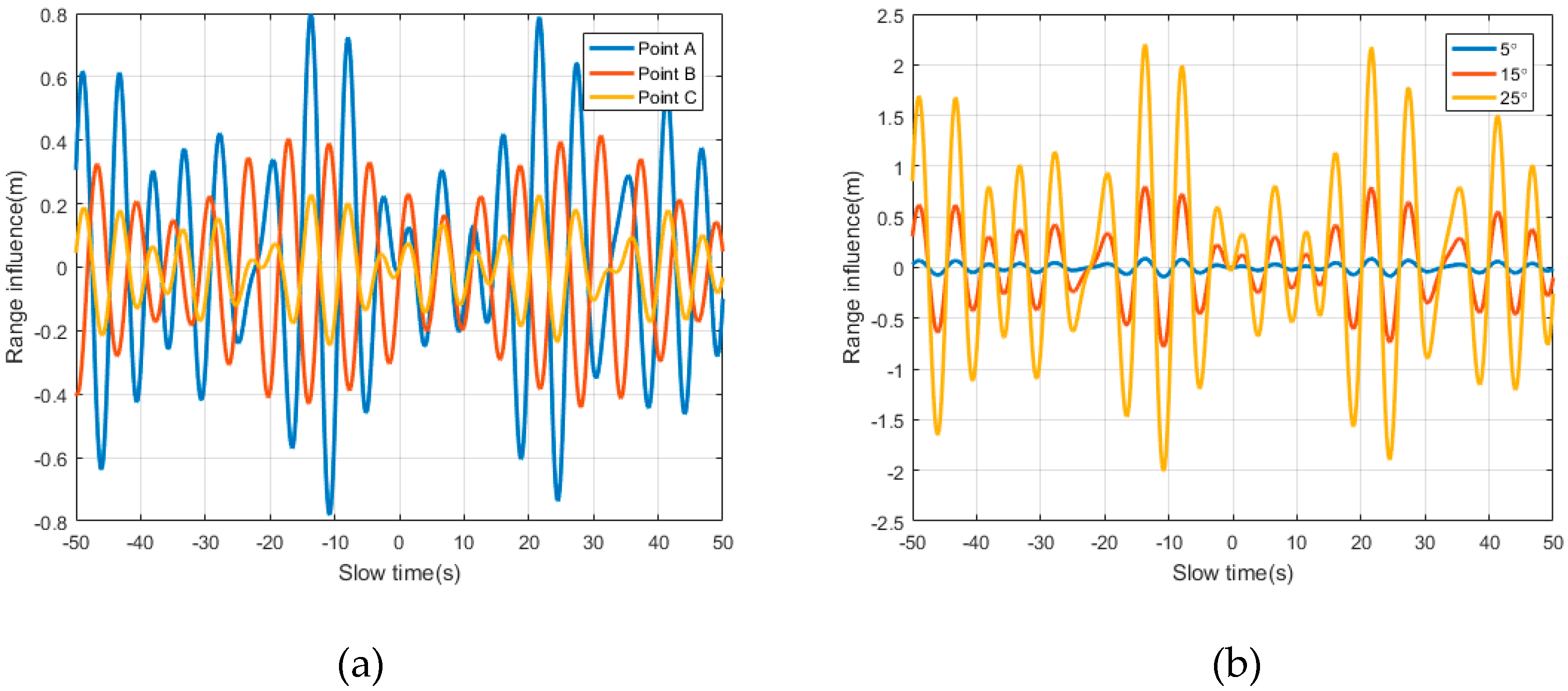
Appendix B. The Influence of Rotation Effect on the Range Cell Migration

As shown in (15), because r i ( t ) is unknown, the influence of rotational motion on range migration is also unknown. The rotation of a ship involves oscillatory motion around the equilibrium point. Furthermore, the resolution of GEO SAR (optimal ρ r _ b e s t = 5   m ) is not high compared with that of the Low Earth Orbit SAR (LEO SAR). The simulation of the influence of rotational motion on the slant range is shown in Figure A3. The rotational motion parameters, except Θ r , p , y , are listed in Table A1; the parameters of the positions of the scatter points in a ship are listed in Table A2.
Table A2. The parameters of the positions of scatter points.
SpecificationsValue
The ship’s coordinate system O B P Z , m b i p i z i
Scatter point A10010010
Scatter point B−50−256
Scatter point C25−155
Figure A3. The influence of rotational motion on the slant range: (a) when Θ r , p , y = 15 ° , the influence on scatter points A, B, and C; (b) when Θ r , p , y = 5 ° , 15 ° , and 25 ° , the influence on scatter point A.
Remotesensing 12 02249 g0a3
Figure A3a shows that when all amplitudes of 3D rotation are Θ r , p , y = 15 ° , the influence on the slant range of scatter points A, B, and C is less than ρ r _ b e s t / 2 , i.e., the influence on slant range is less than half of the range resolution, range cell migration will not occur. Furthermore, when a scatter point is farther away from the gravity center, the influence of rotation is greater. So, when the amplitude of 3D rotation is Θ r , p , y = 5 ° , 15 ° , and 25 ° , the influence on scatter point A are as shown in Figure A3b. The simulation results show that a larger amplitude of rotation has a greater influence on the slant range. The influence on the slant range of scatter point A is less than ρ r _ b e s t / 2 , i.e., when Θ r , p , y is less than 25 ° , the influence of 3D rotational motion in GEO SAR does not cause range cell migration for a scatter point whose distance from the gravity center is not further away than scatter point A. In general, it can be considered that rotational motion does not cause range cell migration in GEO SAR.

References

  1. Skolnik, M. Radar Handbook, 3rd ed.; IEEE: Piscataway, NJ, USA, 2008; pp. 129–130. [Google Scholar]
  2. Stephan, B.; Lehner, S.; Fritz, T.; Soccorsi, M.; Soloviev, A.; van Schie, B. Ship Surveillance with Terrasar-X. IEEE Transact. Geosci.Remote Sens. 2011, 49, 1092–1103. [Google Scholar]
  3. Song, S.; Xu, B.; Yang, J. Ship Detection in Polarimetric SAR Images via Variational Bayesian Inference. IEEE J. Sel. Top. Appl. Earth Obs. Remote Sens. 2017, 10, 2819–2829. [Google Scholar] [CrossRef]
  4. Ao, W.; Xu, F.; Li, Y.; Wang, H. Detection and Discrimination of Ship Targets in Complex Background From Spaceborne ALOS-2 SAR Images. IEEE J. Sel. Top. Appl. Earth Obs. Remote Sens. 2018, 11, 536–550. [Google Scholar] [CrossRef]
  5. Pelich, R.; Longépé, N.; Mercier, G.; Hajduch, G.; Garello, R. Vessel Refocusing and Velocity Estimation on SAR Imagery Using the Fractional Fourier Transform. IEEE Trans. Geosci. Remote Sens. 2015, 54, 1670–1684. [Google Scholar] [CrossRef]
  6. Madsen, S.; Edelstein, W.; di Domenico, L.D.; Labrecque, J. A geosynchronous synthetic aperture radar; for tectonic mapping, disaster management and measurements of vegetation and soil moisture. In Proceedings of the IGARSS 2001, Scanning the Present and Resolving the Future. Proceedings. IEEE 2001 International Geoscience and Remote Sensing Symposium (Cat. No.01CH37217); Institute of Electrical and Electronics Engineers (IEEE): Piscataway, NJ, USA, 2002. [Google Scholar]
  7. NASA; JPL. Global Earthquake Satellite System: A 20-Year Plan to Enable Earthquake Prediction; California Institute of Technology: Pasadena, CA, USA, 2003.
  8. Bruno, D.; Hobbs, S. Radar Imaging From Geosynchronous Orbit: Temporal Decorrelation Aspects. IEEE Trans. Geosci. Remote Sens. 2010, 48, 2924–2929. [Google Scholar] [CrossRef]
  9. Ruiz-Rodon, J.; Broquetas, A.; Makhoul, E.; Guarnieri, A.M.; Rocca, F. Nearly Zero Inclination Geosynchronous SAR Mission Analysis With Long Integration Time for Earth Observation. IEEE Trans. Geosci. Remote Sens. 2014, 52, 6379–6391. [Google Scholar] [CrossRef]
  10. Hobbs, S.; Mitchell, C.N.; Forte, B.; Holley, R.; Snapir, B.; Whittaker, P. System Design for Geosynchronous Synthetic Aperture Radar Missions. IEEE Trans. Geosci. Remote Sens. 2014, 52, 7750–7763. [Google Scholar] [CrossRef] [Green Version]
  11. Li, Y.; Guarnieri, A.M.; Hu, C.; Rocca, F. Performance and Requirements of GEO SAR Systems in the Presence of Radio Frequency Interferences. Remote Sens. 2018, 10, 82. [Google Scholar] [CrossRef] [Green Version]
  12. Fuster, R.M.; Usón, M.F.; Ibars, A.B. Interferometric orbit determination for geostationary satellites. Sci. China Inf. Sci. 2017, 60, 060302. [Google Scholar] [CrossRef] [Green Version]
  13. Hu, C.; Long, T.; Zeng, T.; Liu, F.; Liu, Z. The Accurate Focusing and Resolution Analysis Method in Geosynchronous SAR. IEEE Trans. Geosci. Remote Sens. 2011, 49, 3548–3563. [Google Scholar] [CrossRef]
  14. Ding, Z.; Shu, B.; Yin, W.; Zeng, T.; Long, T. A Modified Frequency Domain Algorithm Based on Optimal Azimuth Quadratic Factor Compensation for Geosynchronous SAR Imaging. IEEE J. Sel. Top. Appl. Earth Obs. Remote Sens. 2015, 9, 1119–1131. [Google Scholar] [CrossRef]
  15. Sun, G.; Xing, M.; Wang, Y.; Yang, J.; Bao, Z. A 2-D Space-Variant Chirp Scaling Algorithm Based on the RCM Equalization and Subband Synthesis to Process Geosynchronous SAR Data. IEEE Trans. Geosci. Remote Sens. 2013, 52, 4868–4880. [Google Scholar] [CrossRef]
  16. Yin, W.; Ding, Z.; Lu, X.; Zhu, Y. Beam scan mode analysis and design for geosynchronous SAR. Sci. China Inf. Sci. 2017, 60, 060306. [Google Scholar] [CrossRef]
  17. Hu, C.; Li, Y.; Dong, X.; Wang, R.; Li, Y. Performance Analysis of L-Band Geosynchronous SAR Imaging in the Presence of Ionospheric Scintillation. IEEE Trans. Geosci. Remote Sens. 2016, 55, 159–172. [Google Scholar] [CrossRef]
  18. Hu, C.; Li, Y.; Dong, X.; Li, Y. Avoiding the Ionospheric Scintillation Interference on Geosynchronous SAR by Orbit Optimization. IEEE Geosci. Remote Sens. Lett. 2016, 13, 1676–1680. [Google Scholar] [CrossRef]
  19. Li, D.; Rodriguez-Cassola, M.; Prats-Iraola, P.; Dong, Z.; Wu, M.; Moreira, A. Modelling of tropospheric delays in geosynchronous synthetic aperture radar. Sci. China Inf. Sci. 2017, 60, 060307. [Google Scholar] [CrossRef]
  20. Hu, C.; Li, Y.; Dong, X.; Long, T. Optimal Data Acquisition and Height Retrieval in Repeat-Track Geosynchronous SAR Interferometry. Remote Sens. 2015, 7, 13367–13389. [Google Scholar] [CrossRef] [Green Version]
  21. Hu, C.; Li, Y.; Dong, X.; Wang, R.; Cui, C. Optimal 3D deformation measuring in inclined geosynchronous orbit SAR differential interferometry. Sci. China Inf. Sci. 2017, 60, 060303. [Google Scholar] [CrossRef]
  22. Hu, C.; Ao, D.; Dong, X.; Cui, C.; Long, T. Impacts of Temporal-Spatial Variant Background Ionosphere on Repeat-Track GEO D-InSAR System. Remote Sens. 2016, 8, 916. [Google Scholar] [CrossRef] [Green Version]
  23. Zheng, W.; Hu, J.; Zhang, W.; Yang, C.; Li, Z.; Zhu, J. Potential of geosynchronous SAR interferometric measurements in estimating three-dimensional surface displacements. Sci. China Inf. Sci. 2017, 60, 060304. [Google Scholar] [CrossRef]
  24. Zhang, Y.; Xiong, W.; Dong, X.; Hu, C. A Novel Azimuth Spectrum Reconstruction and Imaging Method for Moving Targets in Geosynchronous Spaceborne-Airborne Bistatic Multichannel SAR. IEEE Trans. Geosci. Remote Sens. 2020, 1–16. [Google Scholar] [CrossRef]
  25. Zhang, Y.; Xiong, W.; Dong, X.; Hu, C.; Sun, Y. GRFT-Based Moving Ship Target Detection and Imaging in Geosynchronous SAR. Remote Sens. 2018, 10, 2002. [Google Scholar] [CrossRef] [Green Version]
  26. Melzi, M.; Hu, C.; Dong, X.; Li, Y.; Cui, C. Velocity Estimation of Multiple Moving Targets in Single-Channel Geosynchronous SAR. IEEE Trans. Geosci. Remote Sens. 2020, 1–19. [Google Scholar] [CrossRef]
  27. Liu, P.; Jin, Y.-Q. A Study of Ship Rotation Effects on SAR Image. IEEE Trans. Geosci. Remote Sens. 2017, 55, 3132–3144. [Google Scholar] [CrossRef]
  28. Cui, W.; Tian, J.; Xia, X.-G.; Wu, S. An Approach for Parameter Estimation of Maneuvering Targets With Nonlinear Motions. IEEE Trans. Aerosp. Electron. Syst. 2020, 56, 67–83. [Google Scholar] [CrossRef]
  29. Gaffar, M.; Nel, W.; Inggs, M. Selecting Suitable Coherent Processing Time Window Lengths for Ground-Based ISAR Imaging of Cooperative Sea Vessels. IEEE Trans. Geosci. Remote Sens. 2009, 47, 3231–3240. [Google Scholar] [CrossRef]
  30. Martorella, M.; Berizzi, F. Time windowing for highly focused ISAR image reconstruction. IEEE Trans. Aerosp. Electron. Syst. 2005, 41, 992–1007. [Google Scholar] [CrossRef]
  31. Bao, Z.; Sun, C.; Xing, M. Time-frequency approaches to ISAR imaging of maneuvering targets and their limitations. IEEE Trans. Aerosp. Electron. Syst. 2001, 37, 1091–1099. [Google Scholar] [CrossRef]
  32. Wang, Y.; Jiang, Y. ISAR Imaging of Maneuvering Target Based on the L-Class of Fourth-Order Complex-Lag PWVD. IEEE Trans. Geosci. Remote Sens. 2009, 48, 1518–1527. [Google Scholar] [CrossRef]
  33. Xia, X.-G.; Wang, G.; Chen, V. Quantitative SNR analysis for ISAR imaging using joint time-frequency analysis-Short time Fourier transform. IEEE Trans. Aerosp. Electron. Syst. 2002, 38, 649–659. [Google Scholar] [CrossRef]
  34. Wang, Y.; Jiang, Y. ISAR Imaging of a Ship Target Using Product High-Order Matched-Phase Transform. IEEE Geosci. Remote Sens. Lett. 2009, 6, 658–661. [Google Scholar] [CrossRef]
  35. Ding, Z.; Zhang, T.; Li, Y.; Li, G.; Dong, X.; Zeng, T.; Ke, M. A Ship ISAR Imaging Algorithm Based on Generalized Radon-Fourier Transform With Low SNR. IEEE Trans. Geosci. Remote Sens. 2019, 57, 6385–6396. [Google Scholar] [CrossRef]
  36. Hajduch, G.; le Caillec, J.M.; Garello, R. Airborne high-resolution isar imaging of ship targets at sea. IEEE Trans. Aerosp. Electron. Syst. 2004, 40, 378–384. [Google Scholar] [CrossRef]
  37. Li, C.; Lin, J. Microwave Noncontact Motion Sensing and Analysis; John Wiley & Sons: Hoboken, NJ, USA, 2013. [Google Scholar]
  38. Chen, V.; Li, F.; Ho, S.S.; Wechsler, H. Micro-doppler effect in radar: Phenomenon, model, and simulation study. IEEE Trans. Aerosp. Electron. Syst. 2006, 42, 2–21. [Google Scholar] [CrossRef]
  39. Ruegg, M.; Meier, E.; Nuesch, D. Vibration and Rotation in Millimeter-Wave SAR. IEEE Trans. Geosci. Remote Sens. 2007, 45, 293–304. [Google Scholar] [CrossRef] [Green Version]
  40. Wang, Q.; Pepin, M.; Beach, R.J.; Dunkel, R.; Atwood, T.; Santhanam, B.; Gerstle, W.; Doerry, A.W.; Hayat, M.M. SAR-Based Vibration Estimation Using the Discrete Fractional Fourier Transform. IEEE Trans. Geosci. Remote Sens. 2012, 50, 4145–4156. [Google Scholar] [CrossRef] [Green Version]
  41. Peng, B.; Wei, X.; Deng, B.; Chen, H.; Liu, Z.; Li, X. A Sinusoidal Frequency Modulation Fourier Transform for Radar-Based Vehicle Vibration Estimation. IEEE Trans. Instrum. Meas. 2014, 63, 2188–2199. [Google Scholar] [CrossRef]
  42. Wang, Y.; Wang, Z.; Zhao, B.; Xu, L. Compensation for High-Frequency Vibration of Platform in SAR Imaging Based on Adaptive Chirplet Decomposition. IEEE Geosci. Remote Sens. Lett. 2016, 13, 792–795. [Google Scholar] [CrossRef]
  43. Campbell, J.B.; Pérez, F.; Wang, Q.; Santhanam, B.; Dunkel, R.; Doerry, A.W.; Atwood, T.; Hayat, M.M. Remote Vibration Estimation Using Displaced-Phase-Center Antenna SAR for Strong Clutter Environments. IEEE Trans. Geosci. Remote Sens. 2018, 56, 2735–2747. [Google Scholar] [CrossRef]
  44. Xu, J.; Xia, X.-G.; Peng, S.-B.; Yu, J.; Peng, Y.-N.; Qian, L.-C. Radar Maneuvering Target Motion Estimation Based on Generalized Radon-Fourier Transform. IEEE Trans. Signal Process. 2012, 60, 6190–6201. [Google Scholar] [CrossRef]
  45. Tian, J.; Cui, W.; Wu, S. A Novel Method for Parameter Estimation of Space Moving Targets. IEEE Geosci. Remote. Sens. Lett. 2014, 11, 389–393. [Google Scholar] [CrossRef]
  46. Kong, L.; Li, X.; Cui, G.; Yi, W.; Yang, Y. Coherent Integration Algorithm For A Maneuvering Target With High-Order Range Migration. IEEE Trans. Signal Process. 2015, 63, 1. [Google Scholar] [CrossRef]
  47. Doerry, A.W. Ship Dynamics for Maritime ISAR Imaging; Sandia National Laboratories: Livermore, CA, USA, 2008. [Google Scholar]
  48. Bäckström, V.; Skarbratt, A. Maritime ISAR Imaging with Airborne Radar. Master’s Thesis, Chalmers University of Technology, Gothenburg, Sweden, 2010. [Google Scholar]
  49. Perry, R.; di Pietro, R.; Fante, R. SAR imaging of moving targets. IEEE Trans. Aerosp. Electron. Syst. 1999, 35, 188–200. [Google Scholar] [CrossRef]
  50. Droitcour, A.; Boric-Lubecke, O.; Lubecke, V.; Lin, J.; Kovacs, G. Range Correlation and I/QI/Q Performance Benefits in Single-Chip Silicon Doppler Radars for Noncontact Cardiopulmonary Monitoring. IEEE Trans. Microw. Theory Tech. 2004, 52, 838–848. [Google Scholar] [CrossRef]
  51. Yan, Y.; Cattafesta, L.; Li, C.; Lin, J. Analysis of Detection Methods of RF Vibrometer for Complex Motion Measurement. IEEE Trans. Microw. Theory Tech. 2011, 59, 3556–3566. [Google Scholar] [CrossRef]
  52. Wang, R.; Hu, C.; Fu, X.; Long, T.; Zeng, T. Micro-Doppler measurement of insect wing-beat frequencies with W-band coherent radar. Sci. Rep. 2017, 7, 1396. [Google Scholar] [CrossRef] [Green Version]
  53. Gao, G.; Ouyang, K.; Luo, Y.; Liang, S.; Zhou, S. Scheme of Parameter Estimation for Generalized Gamma Distribution and Its Application to Ship Detection in SAR Images. IEEE Trans. Geosci. Remote Sens. 2016, 55, 1–21. [Google Scholar] [CrossRef]
Figure 1. The geometry of a rotating ship.
Remotesensing 12 02249 g001
Figure 2. The geometry of a ship and a Geosynchronous Synthetic Aperture Radar (GEO SAR).
Remotesensing 12 02249 g002
Figure 3. The multiple sinusoidal function matching-based ship imaging procedure.
Remotesensing 12 02249 g003
Figure 4. The signal focused at sinusoidal function frequencies in the RD domain.
Remotesensing 12 02249 g004
Figure 5. Compensation for the influence of each sinusoidal function separately.
Remotesensing 12 02249 g005aRemotesensing 12 02249 g005b
Figure 6. The imaging results without rotation matching.
Remotesensing 12 02249 g006
Figure 7. The echo signals after range compression: (a) without the Generalized Keystone Transform (GKT) and Generalized Dechirp Process (GDP); (b) with the GKT and GDP.
Remotesensing 12 02249 g007
Figure 8. The echo signal in the Doppler domain.
Remotesensing 12 02249 g008
Figure 9. The signal after the compensation of each sinusoidal function: (a) 1st sinusoidal function; (b) 2nd sinusoidal function; (c) 3rd sinusoidal function.
Remotesensing 12 02249 g009
Figure 10. The imaging results with rotational motion matching.
Remotesensing 12 02249 g010
Figure 11. Range profile and azimuth profile of the imaging result: (a) the range profile (b) the azimuth profile.
Remotesensing 12 02249 g011
Figure 12. The imaging of a rotating ship: (a) without matching the rotation effect; (b) with the proposed method.
Remotesensing 12 02249 g012
Table 1. The system parameters of GEO SAR.
SpecificationsValueSpecificationsValue
Argument of the perigee270°Pulse bandwidth, B s , MHz 18
Longitude of the ascending node113°Receiver bandwidth, B r , MHz 20
Mean AnomalyPulse Repetition Frequency(PRF), f p , Hz 300
Orbit height, km 36,000Coherent Processing Interval (CPI), T C P I , s 100
Orbit inclination53°Pulse width, T p , μ s 20
Orbit eccentricityThe grazing angle, φ g 60°
Wavelength, λ , m 0.24The angle between the slant range and the B -axis, φ c s 110°
Table 2. The parameters of the rotational motion of the ship.
SpecificationsValue
RollPitchYaw
The amplitudes of 3D rotation, Θ r , p , y , rad0.0873
(5°)
0.0698
(4°)
0.0698
(4°)
The frequencies of 3D rotation, f r , p , y , Hz1/201/141/36
The initial phases of 3D rotation, φ r , p , y , rad0.5236
(30°)
0.8727
(50°)
0
(0°)
Table 3. The parameters of the matched values of sinusoidal functions.
SpecificationsValue
1st2nd3rd
The frequencies, f ^ n , Hz0.1000.0560.144
The amplitudes, Θ ^ i , n , rad0.0940.0700.011
The initial phases, φ ^ n , rad2.6181.5710.005
Table 4. The coordinates of five scatter points.
SpecificationsValue
Coordinate system O B P Z , m b i p i z i
Scatter point A501205
Scatter point B–1001000
Scatter point C30–908
Scatter point D–120–1109
Scatter point E000
Table 5. The matched values of sinusoidal functions for a rotating ship.
SpecificationsValue
1st2nd3rd
The frequencies, f ^ n , Hz0.1000.0560.144
The initial phases, φ ^ n , rad2.6181.5710.005
The amplitudes of scatter point A, Θ ^ 1 , n , rad0.1040.0660.011
The amplitudes of scatter point B, Θ ^ 2 , n , rad0.0940.0700.011
The amplitudes of scatter point C, Θ ^ 3 , n , rad0.0970.0570.012
The amplitudes of scatter point D, Θ ^ 4 , n , rad0.1180.0530.003
The amplitudes of scatter point E, Θ ^ 5 , n , rad0.0010.0000.001

