Atmospheric Correction Thresholds for Ground-Based Radar Interferometry Deformation Monitoring Estimated Using Time Series Analyses

Abstract

Ground-based radar interferometry (GBSAR) is a useful method to control the stability of engineering objects and elements of geographical spaces at risk of deformation or displacement. To secure accurate and credible measurement results, it is crucial to consider atmospheric conditions as they influence the corrections to distance measurements. These conditions are especially important considering the radar bandwidth used. Measurements for the stability of engineering objects are not always performed in locations where meteorological monitoring is prevalent; however, information about the range of variability in atmospheric corrections is always welcome. The authors present a hybrid method to estimate the probable need of atmospheric corrections, which allows partly eliminating false positive alarms of deformations as caused by atmospheric fluctuations. Unlike the numerous publications on atmospheric reductions focused on the current state of the atmosphere, the proposed solution is based on applying a classic machine learning algorithm designed for the SARIMAX (Seasonal Autoregressive Integrated Moving Average with covariate at time) time series data model for satellite data shared by NASA (National Aeronautics and Space Administration) during the Landsat MODIS (Moderate Resolution Imaging Spectroradiometer) mission before performing residual estimation during the monitoring phase. Example calculations (proof of concept) were made for ten-year satellite data covering a region for experimental flood bank stability observations as performed using the IBIS-L (Image by Interferometric Survey—Landslide) radar and for target monitoring data (ground measurements).

1. Introduction

Ground-based radar interferometry (GBSAR) technology has been intensely developed in recent decades and is used to monitor displacements or deformations of buildings and engineering objects [1,2,3], as well as the movement of mass landslides on earthen and rocky mountainsides as caused by different factors [4,5]. This technique has been applied to monitor volcanic and earthquake-prone regions [6]. A considerable portion of the existing scientific studies has indicated that GBSAR can be used to monitor glacier movement [7] or even snowfall mass thickness [8]. This wide range of uses and equipment was reviewed by Monserrat [9]. Huang [10] conducted GBSAR observations in continuous and non-continuous measurement modes. Based on the work of Crosetto [9], continuous measurements are defined as when a unit is installed permanently in one place and performs continuous (every few minutes) long-term (weekly or monthly) measurements. Non-continuous measurements are for relatively slow movements in a measuring scene and where the designation does not need to be obtained continuously but based on observations made from multiple installations of a radar unit in a particular fixed place. In this context, Wang [11] issued geometric corrections to GBSAR data due to unit reposition, which appears to be very important. They presented solutions to this matter using mutual fitting algorithms for radar scenes as obtained over different periods of non-continuous measurements.

Most of the described literature notes through an analogy to SAR (synthetic aperture radar) satellite data that the variability of atmospheric conditions in a region of radar signal propagation strongly determines the accuracy of the displacement measurements made through SAR observations. Therefore, finding the best methodology to eliminate this factor has been the main focus of several authors as it impairs the credibility of GBSAR measurements. Several studies use works of Zebker [12] and Luzi [8] as a basis as they best describe the correlation between changes in the recording phase and atmosphere parameters. In practice, there are different ways to determine and consider atmospheric corrections. First predominant approach is the observation of ground control points (GCP) [13]. However, this approach requires GCP installations in a radar scene, which is inhibited in real field conditions; hence, there are studies on using second approach-permanent scatters, both natural and parts of infrastructure, found in a scene [14]. Corrections based on meteorological information is third natural approach [15]. As underlined by Iglesias [16], the optimal solution seems to be a hybrid approach that combines all three of these concepts.

Setting spot corrections and linear adjustments are insufficient, especially in mountainous areas where atmospheric factors are strongly conditioned by the topography and altitude. This is why many studies pose questions for the distribution of the modeled atmospheric corrections in observed areas. Huang [10] offered a method of coherent point detection based on an analysis that included entropy modeling for the atmospheric correction field by applying the Delaney algorithm. Another approach appeared in Iglesias [16], where GBSAR observations in the X-series were adjusted based on permanent scatters and meteorological data and a distribution of atmospheric corrections based on a model for manifold regression using coherence (APS-MRM—atmospheric phase screen-multiple-regression model).

The need to model surface field distributions is confirmed by measurements collected in mountainous regions in studies on glacial phenomena. Accurate determination of displacements is achieved by performing surface modeling for atmospheric corrections, which include the altitude as described by Huang [10], corrections give distinct non-continuous measurements where time-atmospheric corrections are crucial to acquire credible displacement data. The necessity of multiple corrections, including altitude and topography factors, for non-continuous measurements is confirmed in the work of Wang [11]. This work used advanced InSAR (interferometric synthetic aperture radar) algorithms for correlation data from different measurement periods (including the non-local “MIAS” method (multi-temporal interferometry based on amplitude similarity)). Many studies using the GBSAR approach repeatedly integrated several different research methods, including photogrammetry and TLS (terrestrial laser scanning) and often combined the validation results with SAR satellite data observations.

This work considers the use of radar satellite data while applying the information for atmospheric conditions. This information serves to estimate the probability of extrapolating the parameters to describe the atmospheric state as well as the resulting apparent displacements as threshold merits when detecting real displacements. In the first part of this study, satellite data provide time series information at monthly intervals over 19 years (2000–2018), in which the merit of observations is the surface temperature of the final day in a given month. Two important attributes of the satellite data are:

• It is possible to analyze time series data for regions where sensors were not located, e.g., temperature data before the region was a focus of interest for object monitoring.
• Satellite data can be easily verified in regard to potential mistakes; thus, one can easily analyze neighboring areas and examine if the trends or merits are similar. Moreover, satellite data are repeatedly verified (are not a unique installation for the area), which provides credible accuracy.

The second part of this work analyzes the ground-based radar interferometry results as acquired during the observations of experimental flood bank flanks. Different flood scenarios were realized on the flood bank after multiple water risings. In this case, the ground-based radar interferometry method, aside from the classic geodesic measurements, provides base measurements to estimate surface deformations in flood bank construction. The atmospheric conditions were precisely monitored during the experiment, which provides time series data for changes in the respective meteorological factors to analyze their influence on the determined construction shifts.

The MODIS and GBSAR data analysis aims to approximate atmospheric corrections based on long time series data. The analysis addresses the question of which time series estimation (ARIMA —autoregressive integrated moving average or SARIMAX) model to apply. This enables the prediction of future atmospheric conditions credibly enough to determine the merit of apparent displacements and eliminate them as a basis for alarm states.

The target use of time series from satellites is to reduce false alarm states when the GBSAR-based system is operating at the installation location. Predicting the future state of the atmosphere will be possible based on the proposed model.

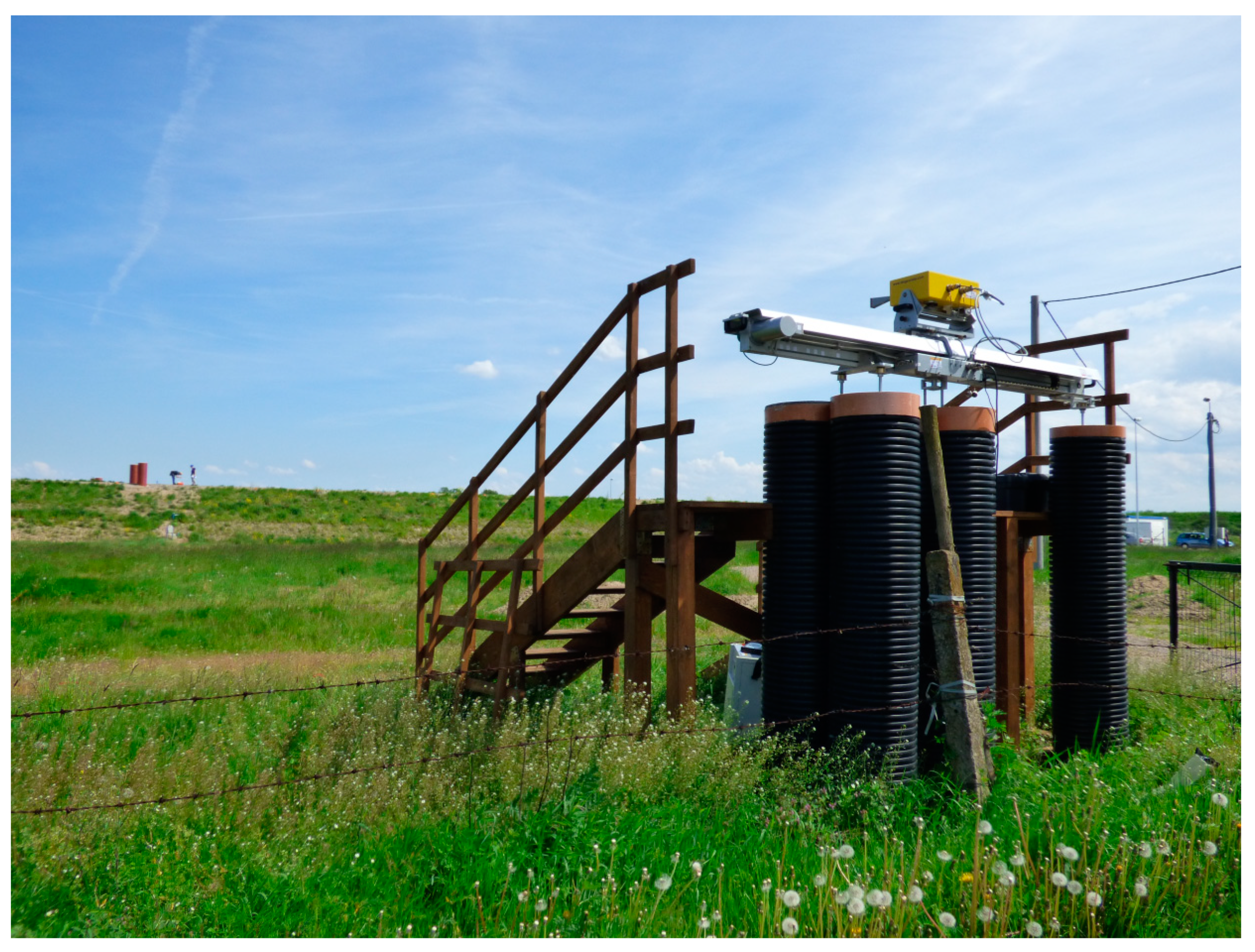
2. Origin and Structure of Measurement Data

The fundamental approach of a well-defined structure monitoring system is to develop methods that collect and analyze information. This allows for the passing of information regarding probable object damage on an assumptive trust level. Monitoring systems will not serve this purpose if they deliver unreliable data, especially if real dangers are missed or if problems are flagged too often when there is no real risk. This work considers the credible estimation of atmospheric correction thresholds that consider data collected to date. The solution has two phases: the first phase is based on the analysis of satellite data collected using the MODIS NASA mission (Wan [17]); the second phase involves the use of atmosphere modeling based on satellite data for measurements made using GBSAR technology. Thus, the analysis results are for the time series data from 2000 until the moment of performing field observation at monthly intervals. This work presents time series data from two layers: daytime land surface temperature and nighttime land surface temperature. NASA delivers satellite scenes over an area of 1200 km by 1200 km in the unit16 format. The MODIS scenes are saved in the hierarchical data format (HDF) as a sinusoidal projection. An example of a satellite scene for the Czernichów municipality near Kraków is given in Figure 1. This region was used as the basis to study features of the north-east region of the middle-east Europe, which is included as part of the experiment.

The research was conducted on a fragment of a 4.5 m flood embankment (Figure 2), which was subjected to variable water levels that reflected the passage of a typical river flood wave. An appropriate network of survey markers equipped with radar reflectors was designed and established. It was of particular importance to determine the displacements in the east–west direction, which is the direction of expected movement based on previous numerical calculations (Stanisz [18]). The experiments included several measurement techniques, such as GBSAR, as performed using the IBIS-L interferometric radar (Figure 3).

The GBSAR technique meets the three main requirements relevant to observations of the earth-filled embankment.

• It is necessary to simultaneously observe multiple points on the surface.
• Continuous observation is required, regardless of the atmospheric and lighting conditions.
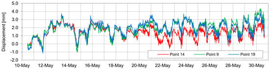
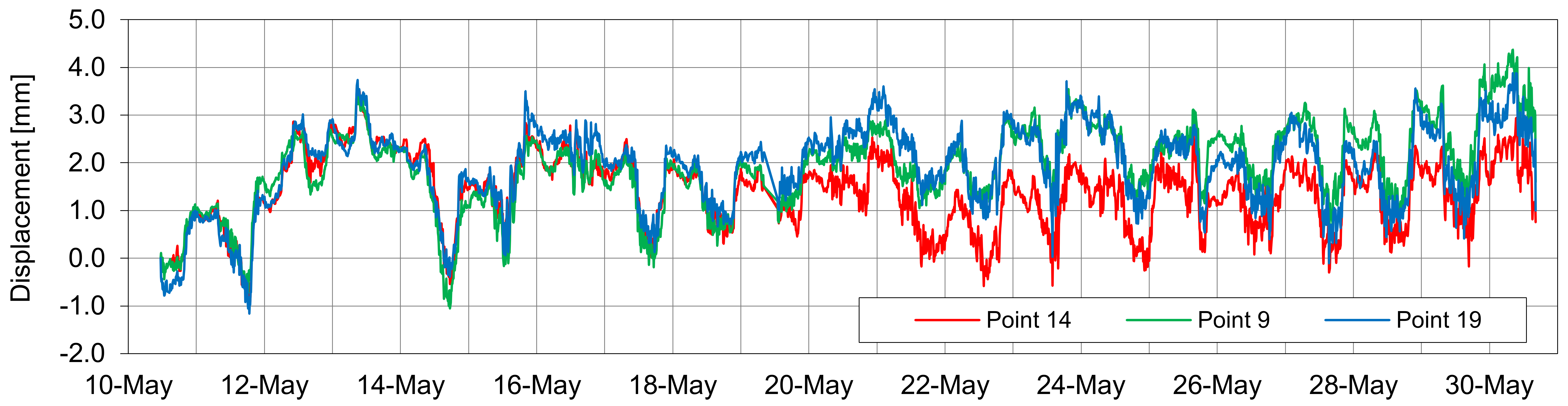
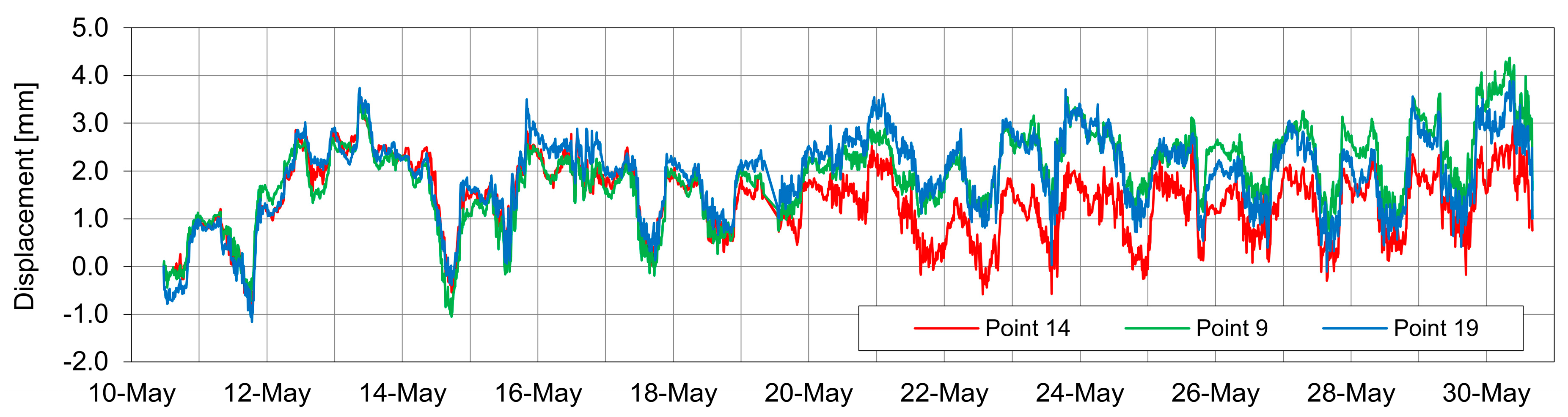
• The expected displacements are on the order of 1 mm; hence, determining the displacement reliably with a measurement error of less than 1 mm must be provided.

Although the various accuracy tests show different displacement measurement accuracy ranging from 0.005 to 2.0 mm (Gentile and Bernardini [19]; Bozzano [20]; Xing [21]), low errors were expected in this work due to:

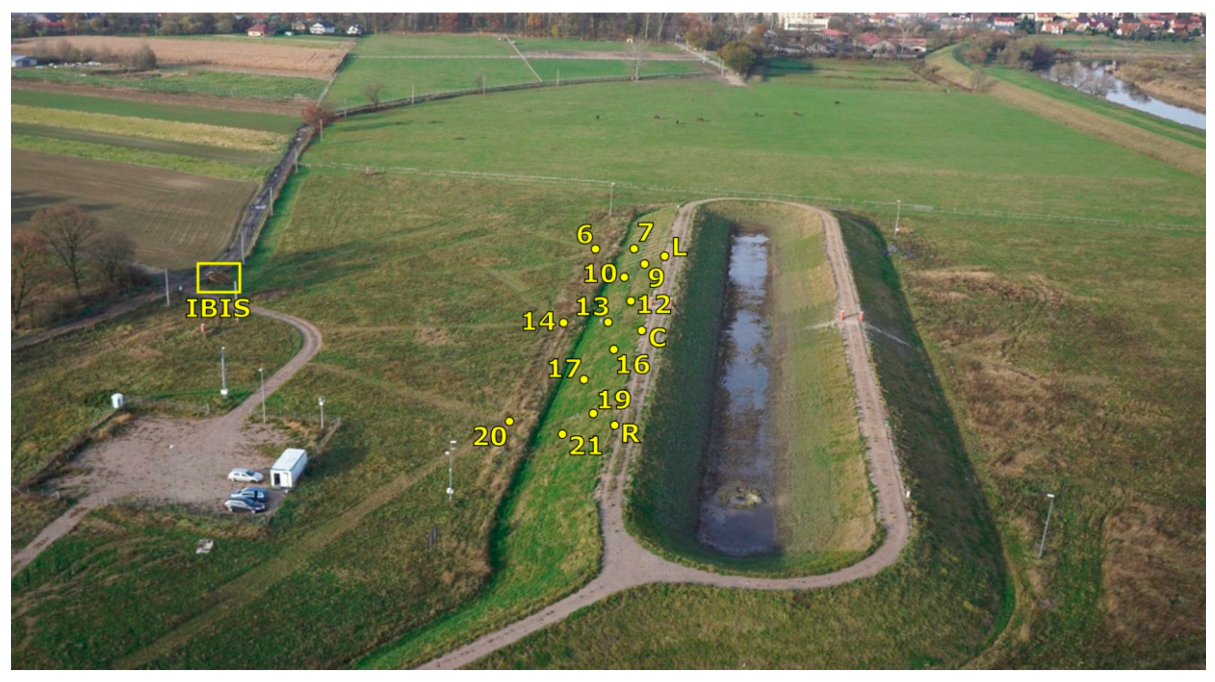
• Use of radar reflectors that significantly increase the signal-to-noise ratio (SNR);
• Relatively short distance (approximately 100 m);
• Acquisition of weather station data for atmospheric corrections.

Figure 4 presents raw displacement records for three selected points. The daily trend is visible and indicates the effects of atmospheric factors with similar variabilities throughout the day. Further processing requires corrections due to the properties of the radar wave propagation medium from the humidity, temperature and pressure.

3. Data Analysis Method and Proposed Solution Algorithm

The HDF data were processed to obtain preliminary and indicative information regarding the temperature ranges in given areas. As the data are rastered over a 1200 km by 1200 km region, the GDAL (Geospatial Data Abstraction Library) library was used to obtain the information for the Czernichów area. The initial file was in the SHP format, which allowed clip operations (excising data) on the MODIS scene, and was processed in the mapping that was compatible with the NASA-accepted model. Figure 5 shows the average daytime and nighttime temperatures for the analyzed area. For consistency, the temperature data are given in Centigrade. The analyzed area where deformation measurements were conducted is located at 49°59′ N latitude and 19°40′ E longitude. Therefore, it is not surprising that the coldest months were December and January and the hottest were July and August.

Our final aim is to estimate the temperature based on pre-existing observations, which are to predict accurate atmospheric corrections. Therefore, the important information in the data is the observed potential deviations from the average in a given month throughout the years. Figure 6 presents the monthly temperature deviations towards the average for the Czernichów area from 2000–2018, as estimated using the MODIS data.

As this work considers time series data, the natural algorithm to solve the problem is the ARIMA model [22]. The ARIMA is a regression model that can be fit to time series data to better understand or predict future points in the series. The ARIMA model adopts the three parameters denoted p, d, and q. The first (p) is the autoregressive component that extracts the effects of previous observations. The second (d) is the parameter responsible for the degree of series integration, which is the basic task to ensure the data are a stationary time series. The third (q) is a term for the moving average, which ties the model error as a linear combination of the observed error from the previous data.

The ARIMA model is appropriate if the p, d, and q parameters are properly chosen; therefore, a stationary time series will be the focus of the analysis. If the analyzed time series is stationary, then d = 0. Hence the AR model is given by:

$$Y_t=\alpha +{\beta }_1{\gamma }_{t-1}+{\beta }_2{\gamma }_{t-2}+\dots +{\beta }_p{\gamma }_{t-p}+{ϵ}_1$$

(1)

while the moving average model is:

$$Y_t=\alpha +{ϵ}_1+{\phi }_1{ϵ}_{t-1}+{\phi }_2{ϵ}_{t-2}+\dots +{\phi }_q{ϵ}_{t-q}$$

(2)

The equation for an ARIMA model where the time series is differenced at least once to ensure stationarity is:

$$Y_t=\alpha +{\beta }_1{\gamma }_{t-1}+{\beta }_2{\gamma }_{t-2}+\dots +{\beta }_p{\gamma }_{t-p}+{ϵ}_1+{\phi }_1{ϵ}_{t-1}+{\phi }_2{ϵ}_{t-2}+\dots +{\phi }_q{ϵ}_{t-q}$$

(3)

where: α—constant, β_i, φ₁—autoregressive and moving average coefficients and p, q—autoregressive and moving average lags.

For the observed data, it is noted that a modification to the standard ARIMA model is needed. Despite integrating the time series (Figure 7), the identification of the correct parameters is not clear because of seasonal effects that appear in the data. It can be stated, however, that the p, d and q factors should be from 0 to 2.

As the data show seasonal characteristics, the factors that evaluate the time series model must be considered. The ARIMA model, as complemented with seasonal influence, is the SARIMAX model. The implementation is called SARIMAX instead of SARIMA because the “X” addition to the method name means that the implementation also supports exogenous variables. This model is specified with

(p, d, q) × (P, D, Q) m

(4)

where:

• p—trend autoregression order
• d—trend difference order
• q—trend moving average order

and

• P—seasonal autoregressive order
• D—seasonal difference order
• Q—seasonal moving average order
• m—the number of time steps for a single seasonal period

For the studied time series, 64 combinations of factors where generated with m = 12 (monthly observations over the year). The best variant of the SARIMAX model was chosen based on the Akaike information criterion (AIC) with the formula:

$$AIC=2k-2\ln \left(\widehat{L}\right)$$

(5)

where k—number of estimated parameters in the model and $\widehat{L}$ is the maximum value of the model likelihood function.

For a given set of candidate models for the MODIS data, the preferred model is the one with a minimum AIC. In our case, the optimum model is the SARIMAX with (p = 1, d = 1, q = 1) × (P = 0, D = 1, Q = 1, m = 12). For this candidate model, the AIC is 1032.14.

During the measurements, the current state of the atmosphere is determined via atmospheric pressure measurements in addition to humidity and temperature measurements. For electro-optic rangefinders, the greatest influence on the atmospheric reduction is potential changes in the temperature as these generally operate in the near infrared or visible bandwidths. For atmospheric reduction techniques that estimate the influence of the atmosphere using distance measurements in the microwave regime, the crucial information is the variability in the humidity.

According to Luzi [23], the influence of the atmosphere on the registered phase reading can be expressed as:

$$\phi =\frac{4\pi }{{\mathsf{\lambda }}_0}r+\frac{4\pi }{{\mathsf{\lambda }}_0}\left(n_{atm}-1\right)r$$

(6)

where:

• ${\lambda }_0=\frac{c}{f_0}$—nominal wavelength
• f₀—nominal frequency
• r—measuring vector
• $n_{atm}$—atmospheric refraction factor

In the case of variable atmospheric parameters (pressure, humidity or temperature), achieving accurate results requires changing the atmospheric refraction factor. This is because measurements taken during variable conditions will affect the phase of the returning signal, even if the measured engineering object was stable and fully preserved the original phase:

$$\mathsf{\Delta }{\phi }_{atm}=\frac{4\pi }{{\lambda }_0}·{\epsilon }_{atm}·r$$

(7)

where:

• r₁ = r₂ = r—measuring vector assuming object stability
• ε_atm = n_atm2—n_atm1—difference in atmospheric refraction factors during the primary and secondary measurements.

Moreover, negative effect of signal decorrelation must be considered in the case of rain, which is especially detrimental to accurate distance measurements. According to Zebker [12], changes in the registered phase of the measured wave caused by atmospheric conditions can be shown using the correlation:

$$\mathsf{\Delta }r=7.76·{10}^{-5}\underset{0}{\overset{R}{{\displaystyle \int }}}\frac{P}{T}dr+3.73·{10}^{-1}\underset{0}{\overset{R}{{\displaystyle \int }}}\frac{e}{T^2}dr$$

(8)

where:

• R—total propagation length in atmosphere
• P—atmospheric pressure [mbar]
• T—temperature [K]
• e—water vapor pressure [mbar]

Constants in this (and analogic) equation are correct with an accuracy of 99.5% for frequencies up to 30 GHz, which is sufficient for nominal changes in the earth atmosphere (Smith [24]). It is generally more convenient at a given measuring position to register the relative humidity rather than the absolute value. A correlation between the relative humidity h and water vapor pressure e in the atmosphere is expressed with the relation (Kraus [25]):

$$e=\frac{hE}{100}, E=6.107·exp\left(\frac{17.27·\left(T-273\right)}{T-35.86}\right)$$

(9)

The analyzed GBSAR data were a time series acquired at hourly intervals for atmospheric observations of the temperature, humidity, and pressure as well as the assumed displacements based on the observations. For each of the four time series, 64 factor combinations were generated with m = 24 (24 h intermittence). The best variant of the SARIMAX model was chosen based on minimizing the AIC [22]. In our case, the optimum models were:

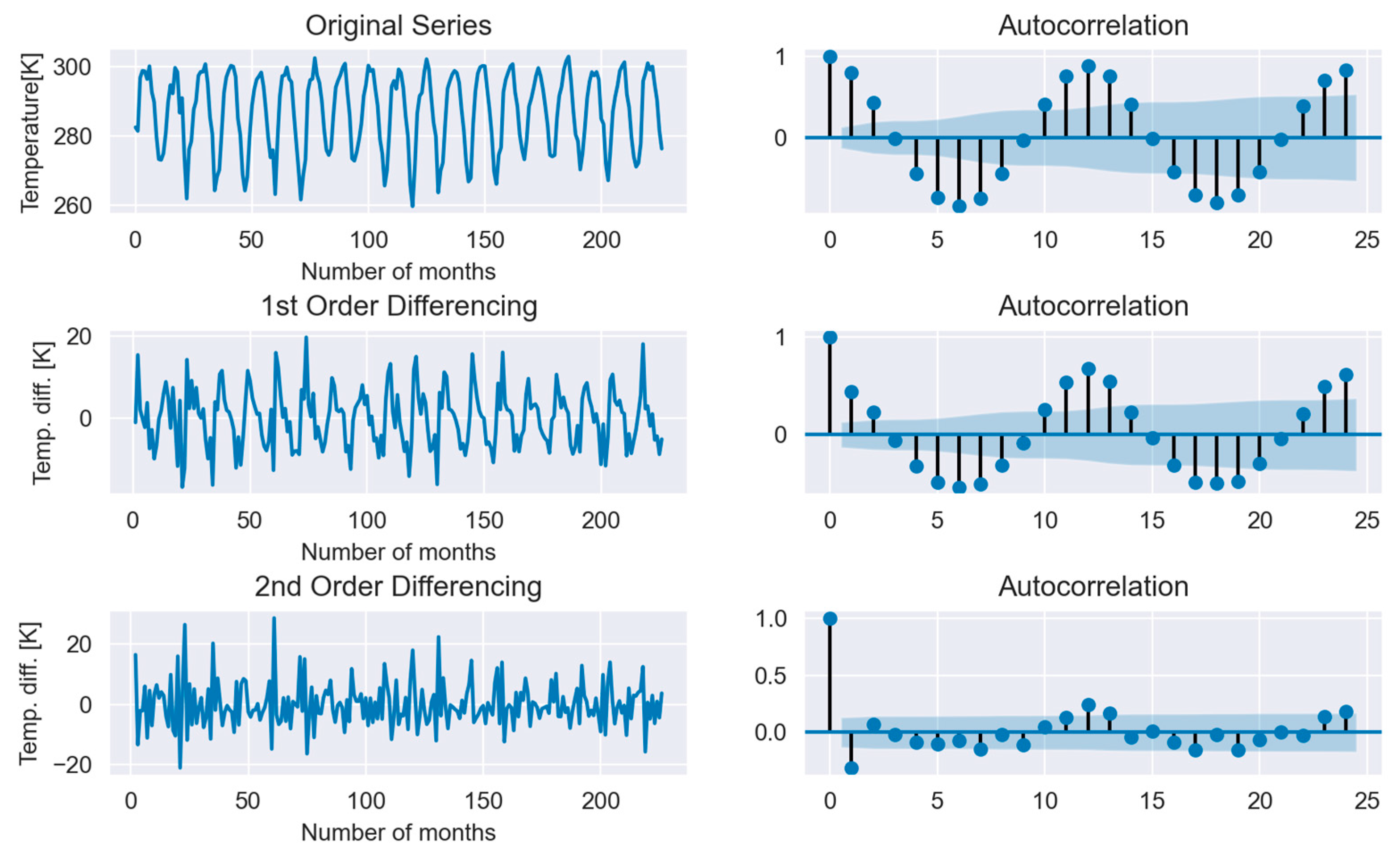
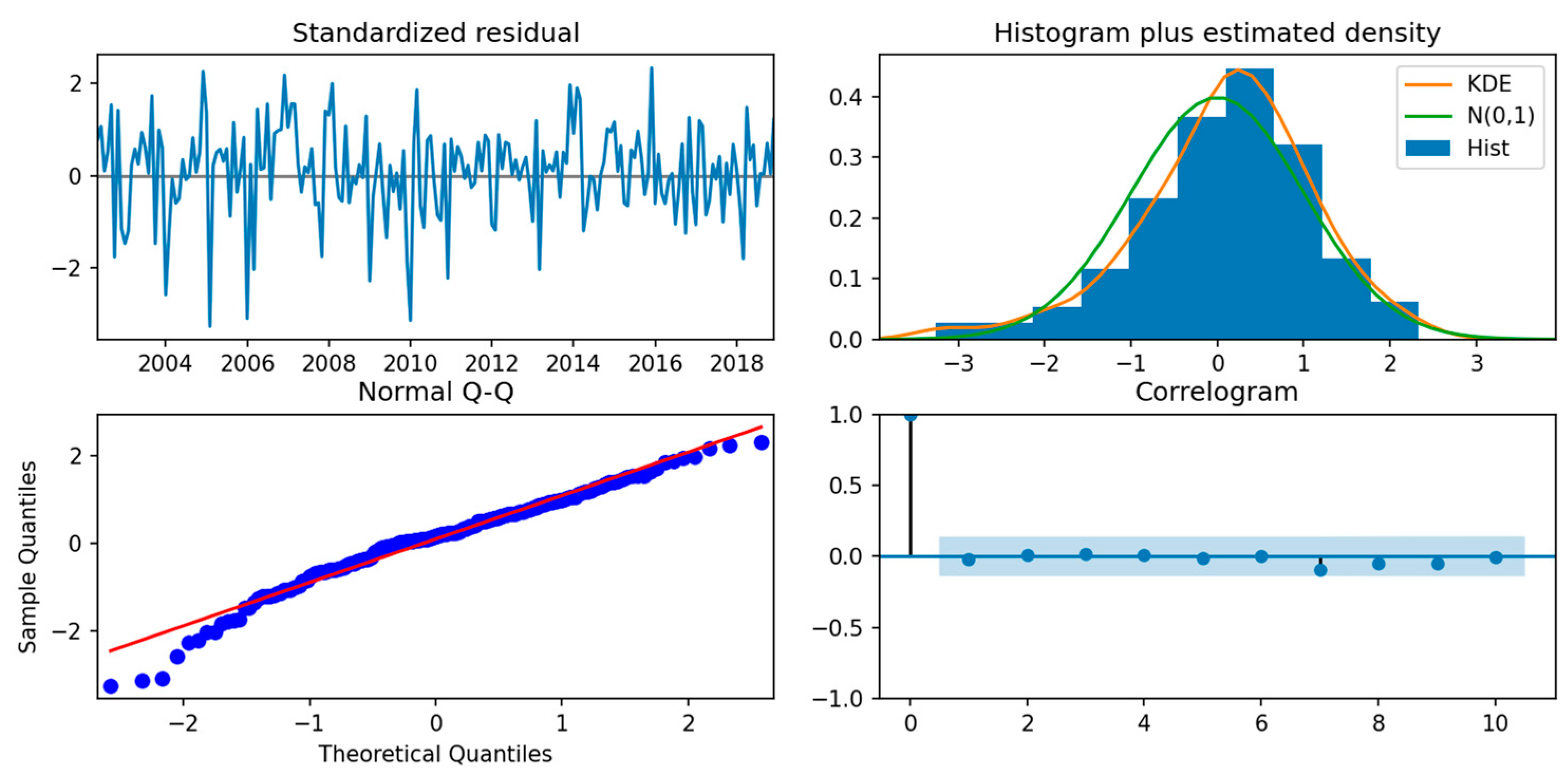
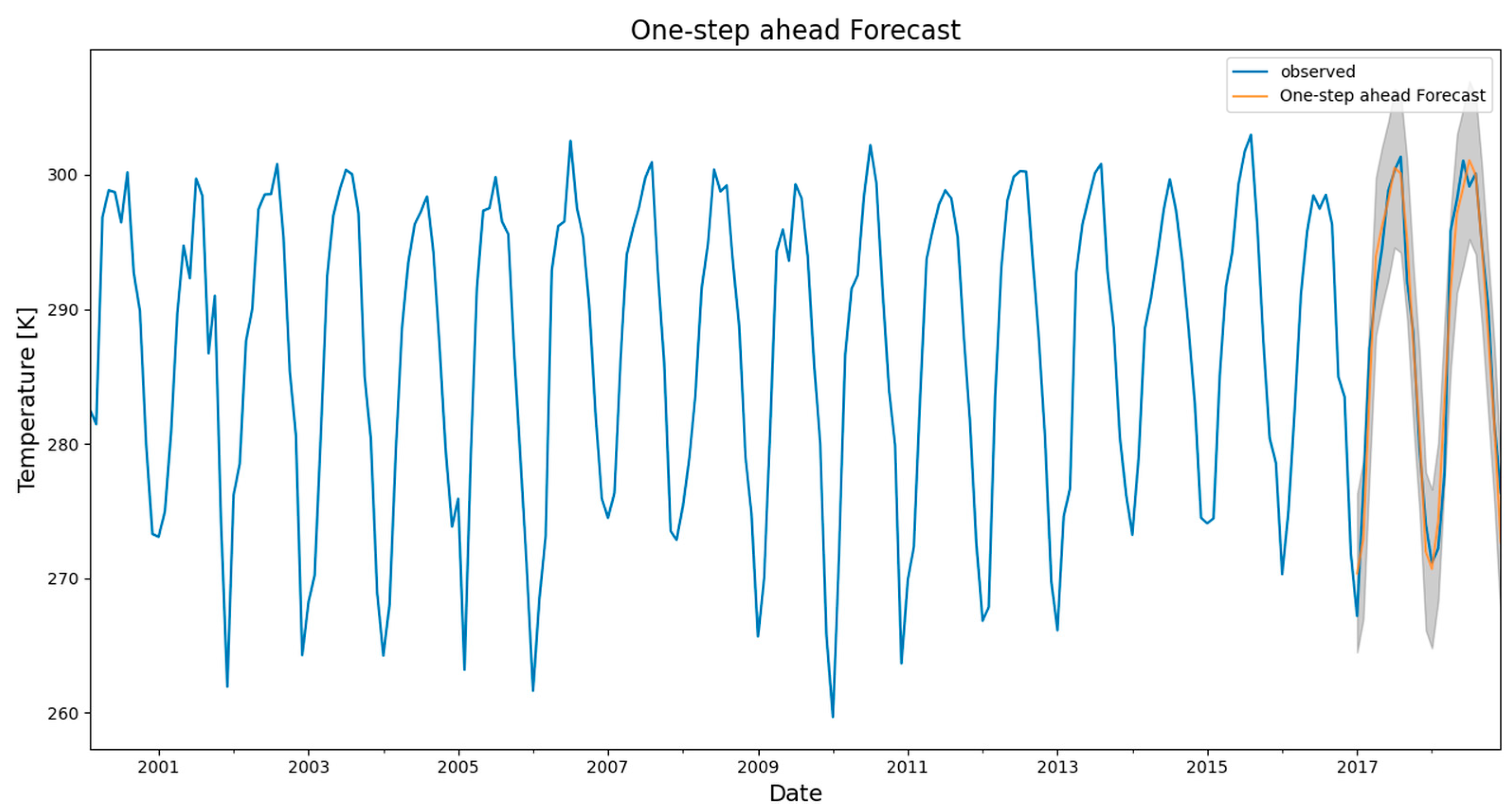
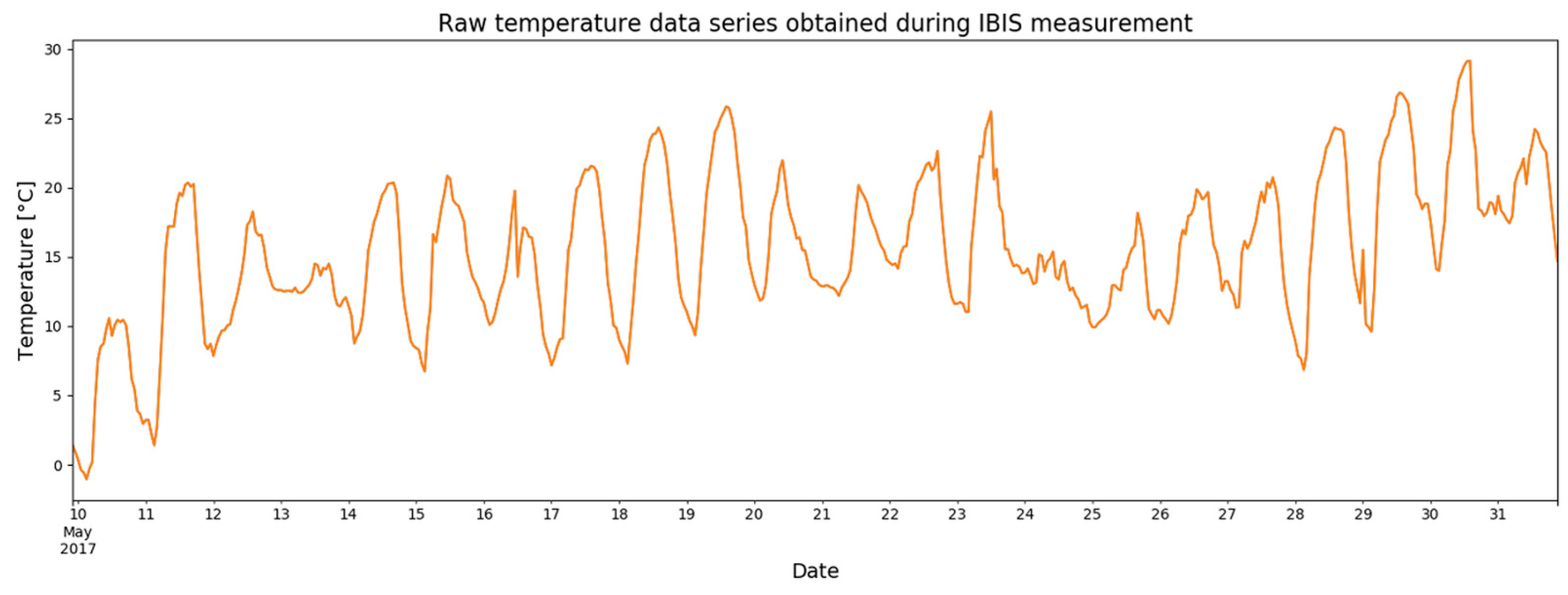
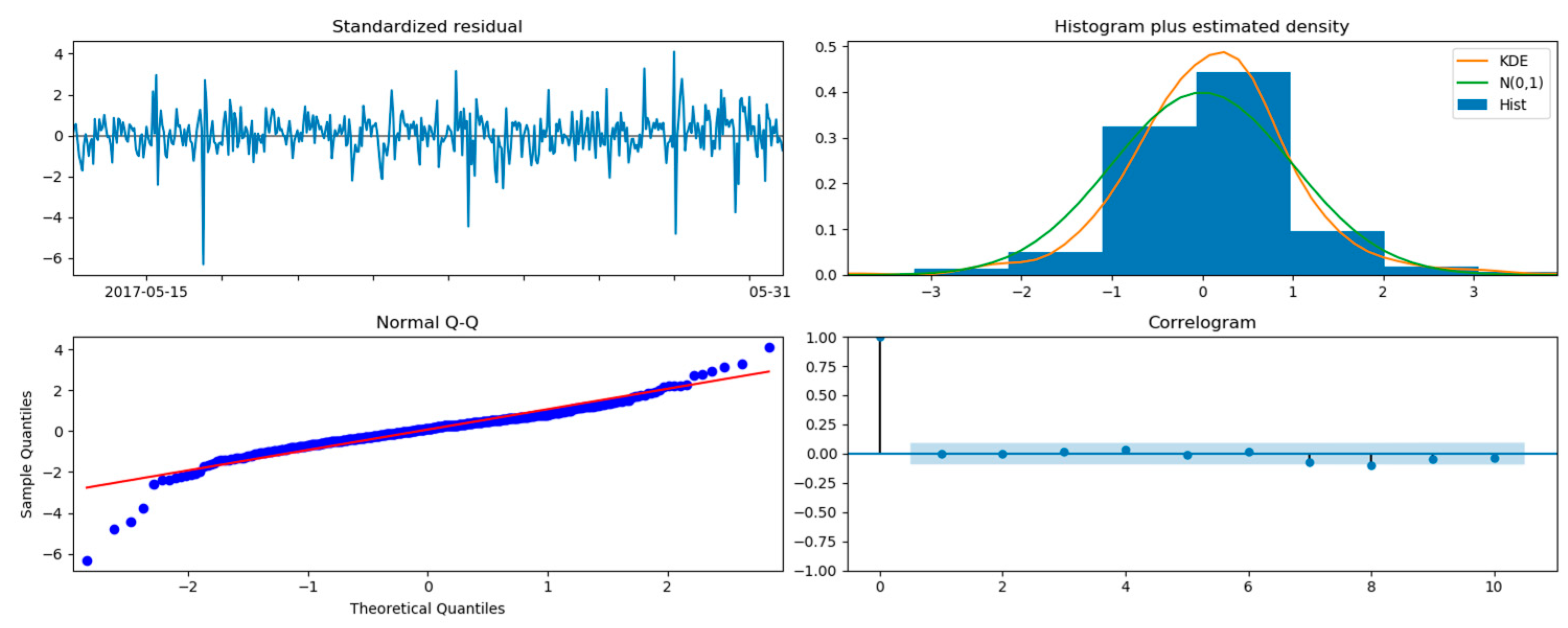
• Temperature data are a SARIMAX (p = 1, d = 0, q = 1) × (P = 0, D = 1, Q = 1, m = 24) with an AIC of 1475.57 (maximum AIC of 4441.75)
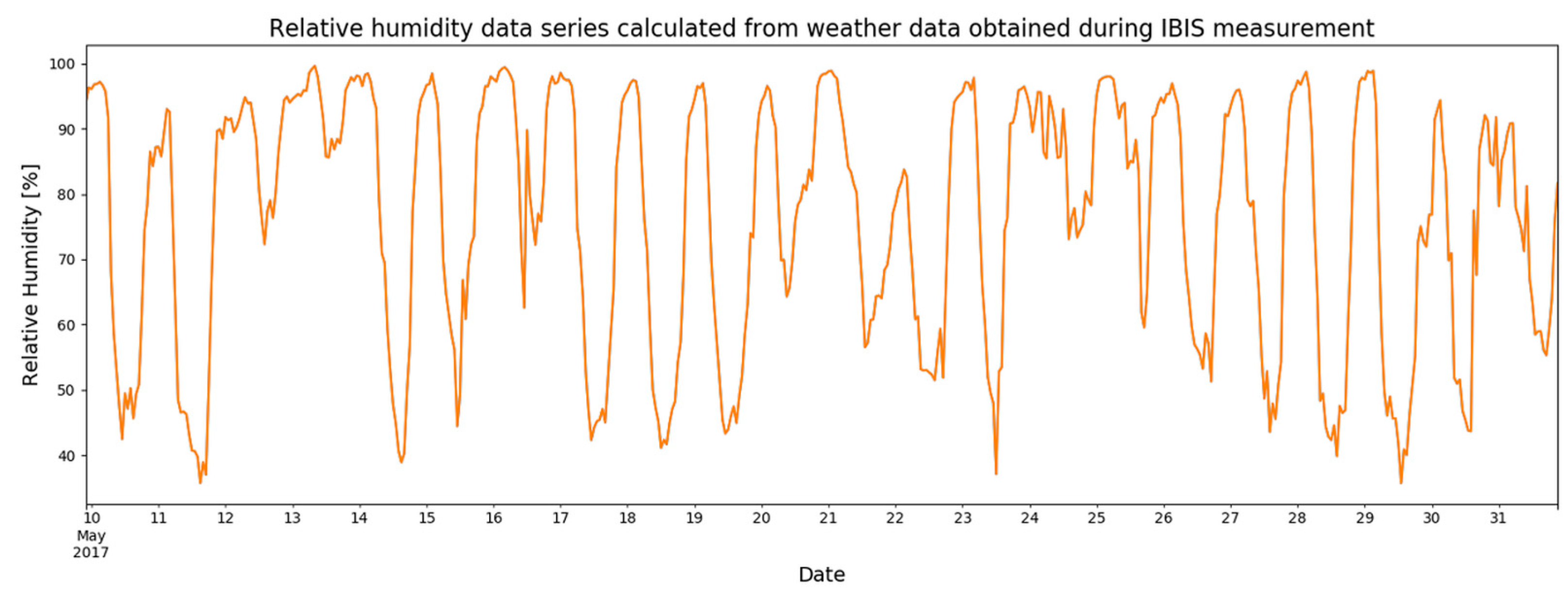
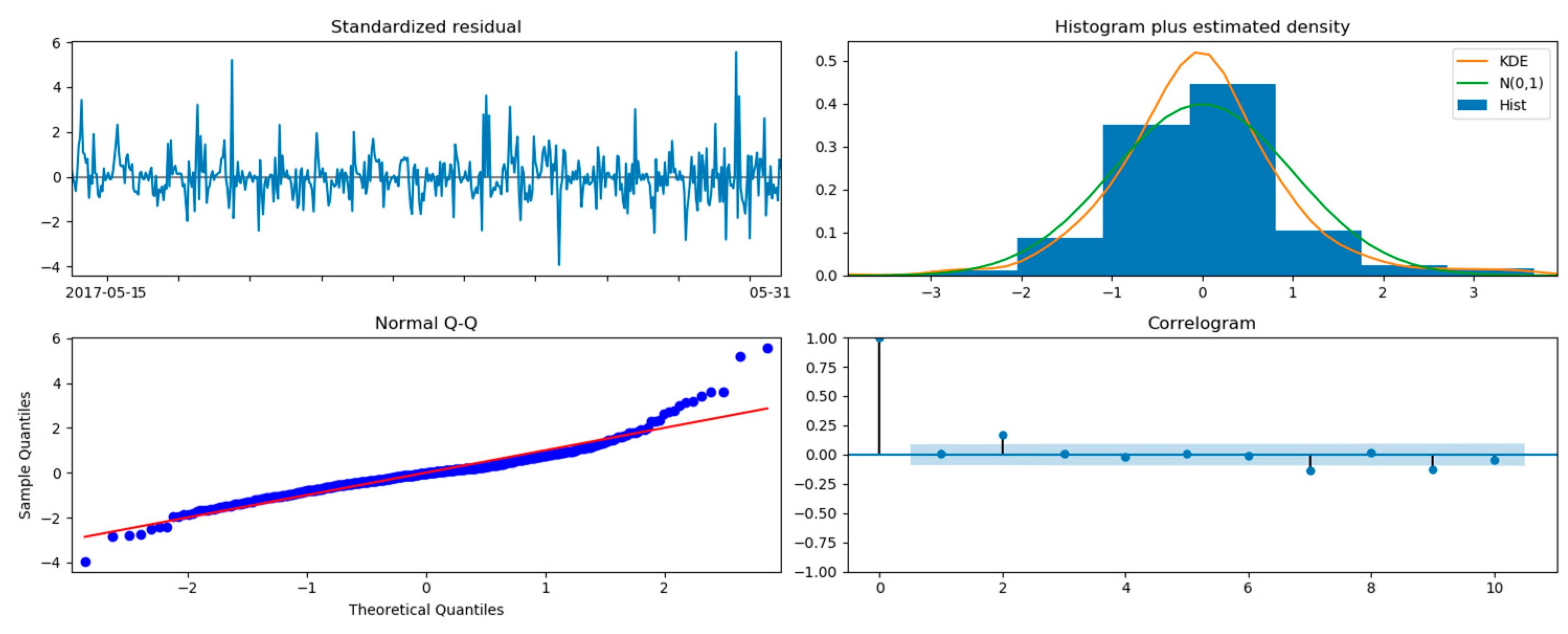
• Relative humidity data are a SARIMAX (p = 1, d = 0, q = 1) × (P = 0, D = 1, Q = 1, m = 24) with an AIC of 2997.11 (maximum AIC of 6097.14)
• Pressure data are a SARIMAX (p = 1, d = 1, q = 0) × (P = 1, D = 0, Q = 1, m = 24) with an AIC of 249.19 (maximum AIC of 8796.48)
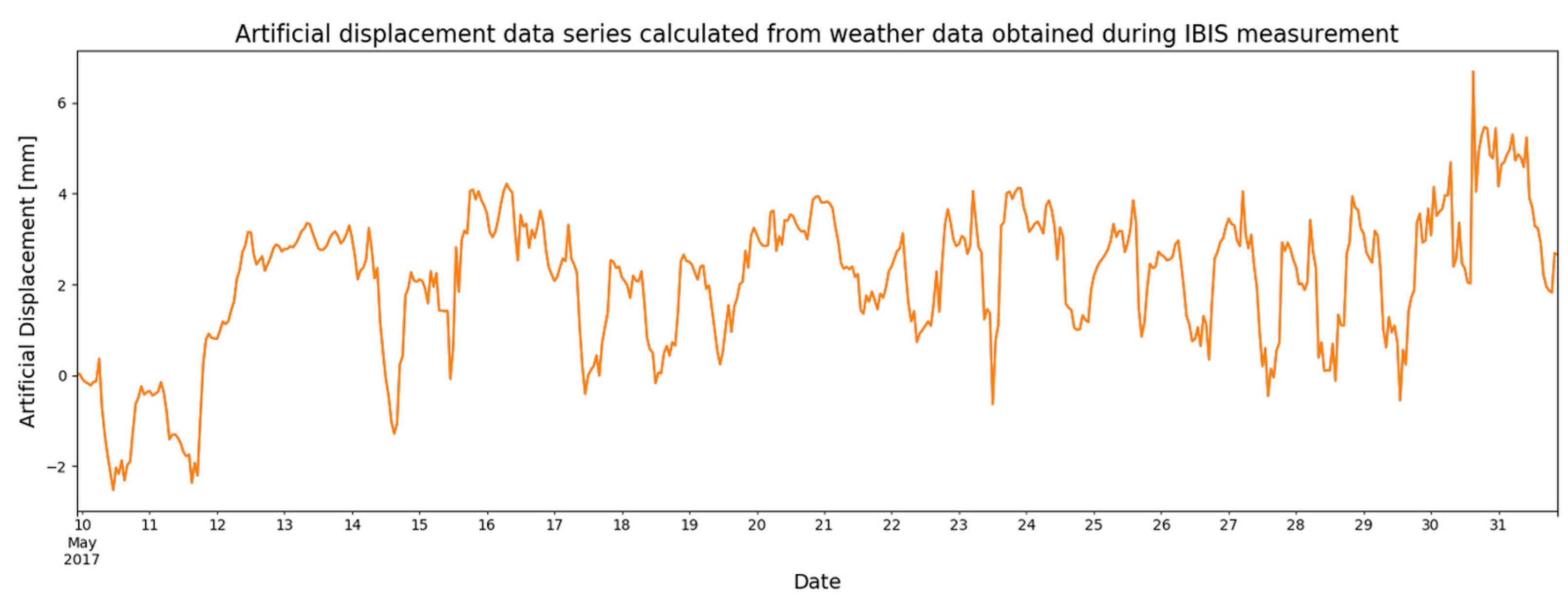
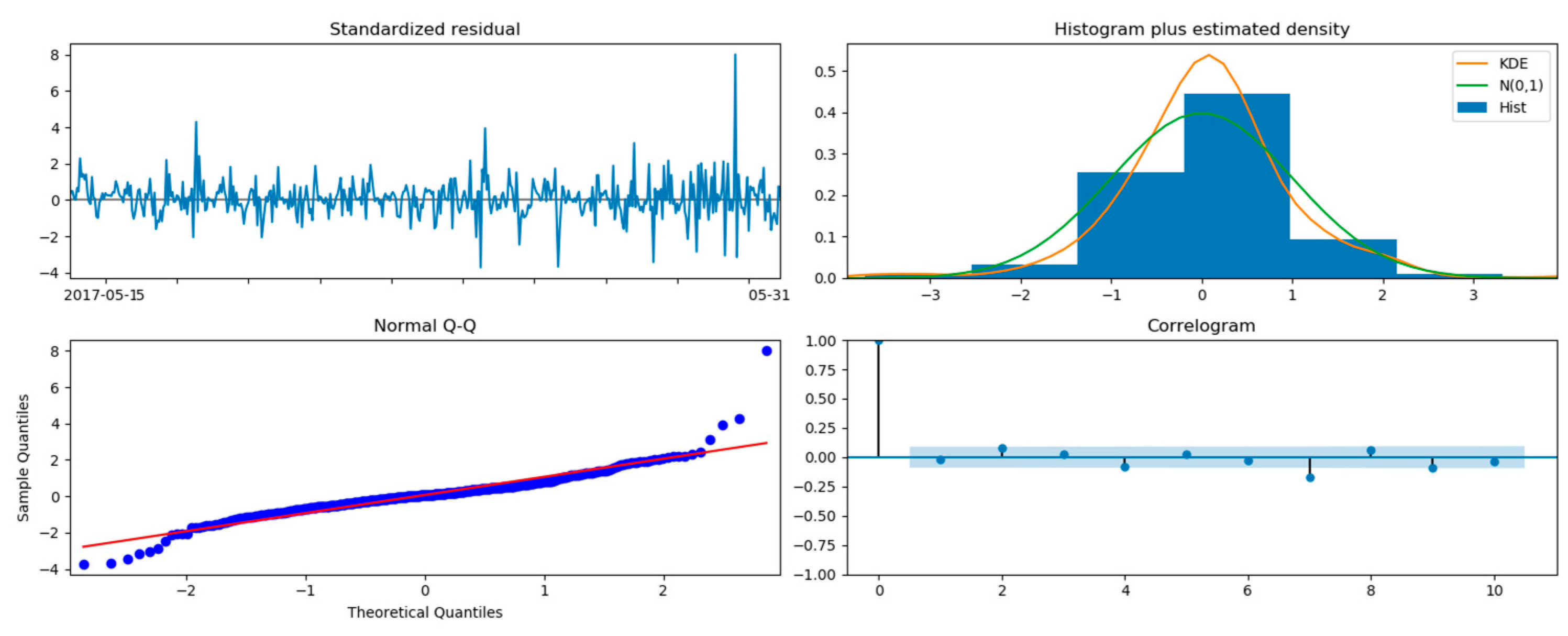
• Apparent displacement pressure data are a SARIMAX (p = 1, d = 0, q = 1) × (P = 0, D = 1, Q = 1, m = 24) with an AIC of 824.93 (maximum AIC of 2506.60)

The results for the sample research task are given by examining the data set with the best fit model. The data from the MODIS HRD files corresponding to the Czernichow region were converted to the json format. The original data are given as a simple plot in Figure 8.

For the data given in Figure 8, four standard diagnostic plots based on the AIC criteria for the SARIMAX model are provided in Figure 9. The standardized residuals plot shows the residuals on the vertical axis and time on the horizontal axis. The points on the residual plot are randomly dispersed about the horizontal axis, suggesting a linear regression model is appropriate for the data. The quantile-quantile graph was created by plotting two sets of quantiles against one another. As both sets of quantiles came from the same distribution, the points form an approximately linear line. The histogram indicates the accuracy of the model as only random errors are present. Finally, the correlogram suggests the given model order is correctly chosen.

The optimal SARMIMAX model was used to predict the temperature using a one-step-ahead method for the data from 2017–2019 based on the model from the 2000–2017 data, as shown in Figure 10. The observed data (blue) coincides with the model data (orange) showing minimal errors. The model data fit into an assumed 95% confidence region (gray). This validates the accuracy of modeling time series data that have a systematic factor (yearly cyclicality).

Next, we examine the set of atmospheric data obtained from the IBIS measurements on the flood embankment using the optimal model. The raw temperature data are shown in Figure 11.

Four standard diagnostic plots for the optimal SARIMAX model based on the AIC criteria are given in Figure 12. Both the estimated density and Quantile–Quantile plots indicate that the given model is accurate, but the correlogram indicates a slight exceedance of the correlation range. Therefore, an additional 729 factor combinations were generated in the range of 0–2 assuming m = 24 (24-h intermittence). In this case, the parameters for the optimal SARIMAX model were (p = 1, d = 0, q = 2) × (P = 0, D = 1, Q = 2), m = 24. For this candidate model, the AIC was 1383.97 (maximum AIP of 4441.75). Figure 12 shows the standard diagnostic graphs generated for the optimized parameters. The results of the predictions meet the quality criteria for the lack of systematic errors. The average rest value is zero, indicating the model is stationary.

Two approaches were applied in the forecasting. First, the subsequent value was predicted in given range by including the real value and not any previous predictions. Second, the forecasted value was predicted in given range using only previously predicted data. The results of the forecasting for optimization over the ranges (0,1] and (0,2] based on the one-step-ahead or static approach are shown in Figure 13, and the dynamic approach is shown in Figure 14. The gray color in each figure represents the confidence region for the predicted values set at a level of (0,2].

Analogous processing was applied for the humidity and pressure time series measurements in the optimization range of the SARIMAX model (0,1]. Figure 15, Figure 16 and Figure 17 show example results based on humidity data.

Based on the accuracy of the SARIMAX algorithm for the data representing the atmospheric state, the authors applied the model to analyze the apparent displacement values. These values are not the result of object shifts but are due to changes in the atmospheric pressure, temperature and humidity. Figure 18 presents the calculated apparent displacements for a 21-day period. In addition, as was done previously, we examine the accuracy of the model for the data and demonstrate that the accepted model order is proper using the 4 standard diagnostic plots (Figure 19).

We present the results of the algorithm for the data that represent the apparent displacement model. The authors acknowledge the high endurance of such a solution despite the fact that the data are only partly periodic in nature (Figure 20). The results of the estimation do not differ much from the registered later real distortions of the displacement measurements and fit within the chosen confidence interval.

Next, we compare the real displacements observed through radar with the apparent displacements from the model. Figure 21 presents the measurements based on the registered atmospheric parameters (black) and the calculations based on the chosen dynamic SARIMAX model (blue). Limits in the forecasted values are given in the figure as blue dotted lines. It is noted that in the time periods chosen for the analysis, the forecasted values reflect the measured values better than the calculations. This may be due to violent changes in the meteorological parameters during forecasting. Nevertheless, the forecasted values are sufficiently convergent with the measurements, which indicates their usefulness when estimating measurement uncertainty in regard to displacement observations.

4. Discussion

To summarize the proposed solution, the complete flowchart of the presented method is given in Figure 22. It includes the following main steps of the procedure.

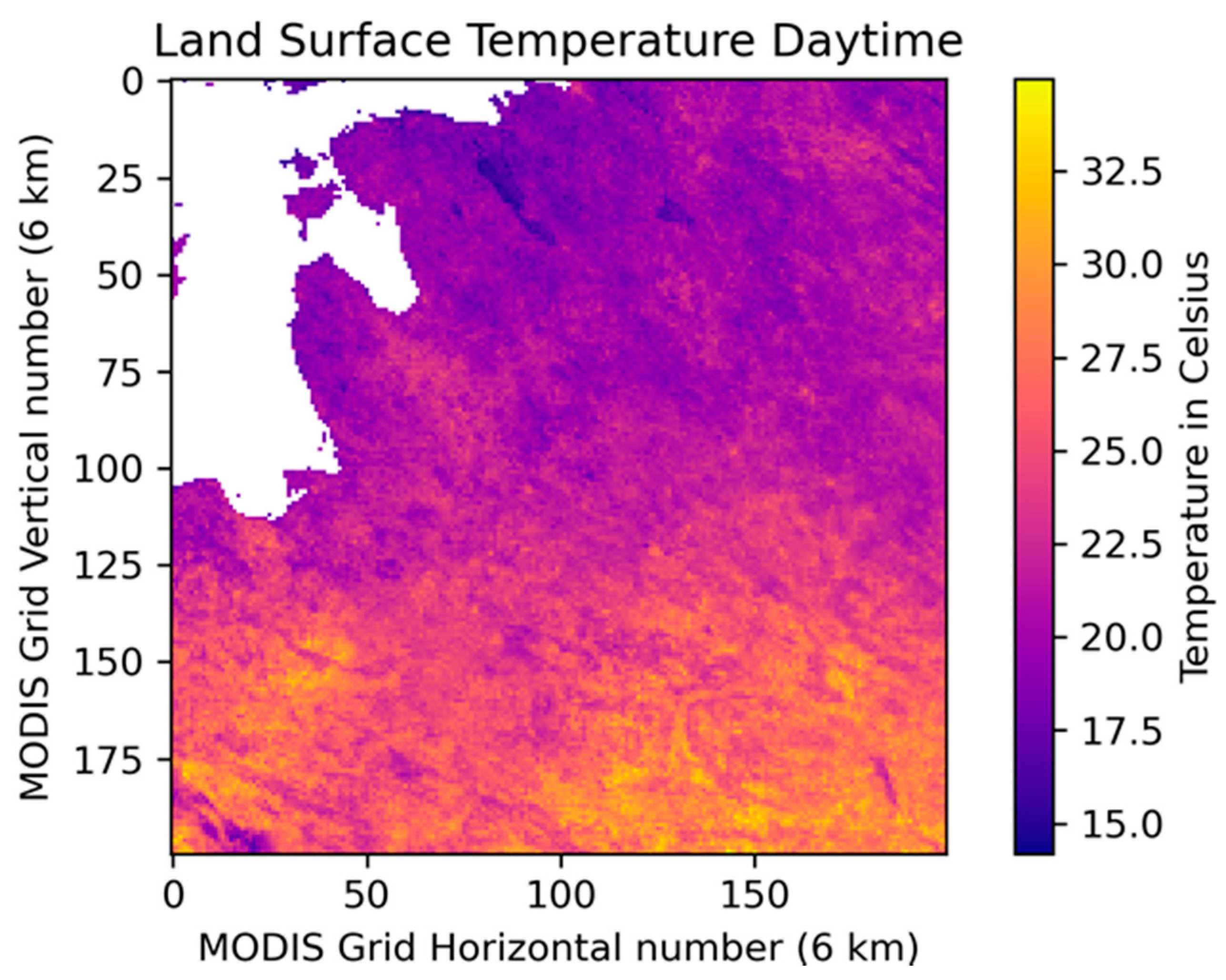
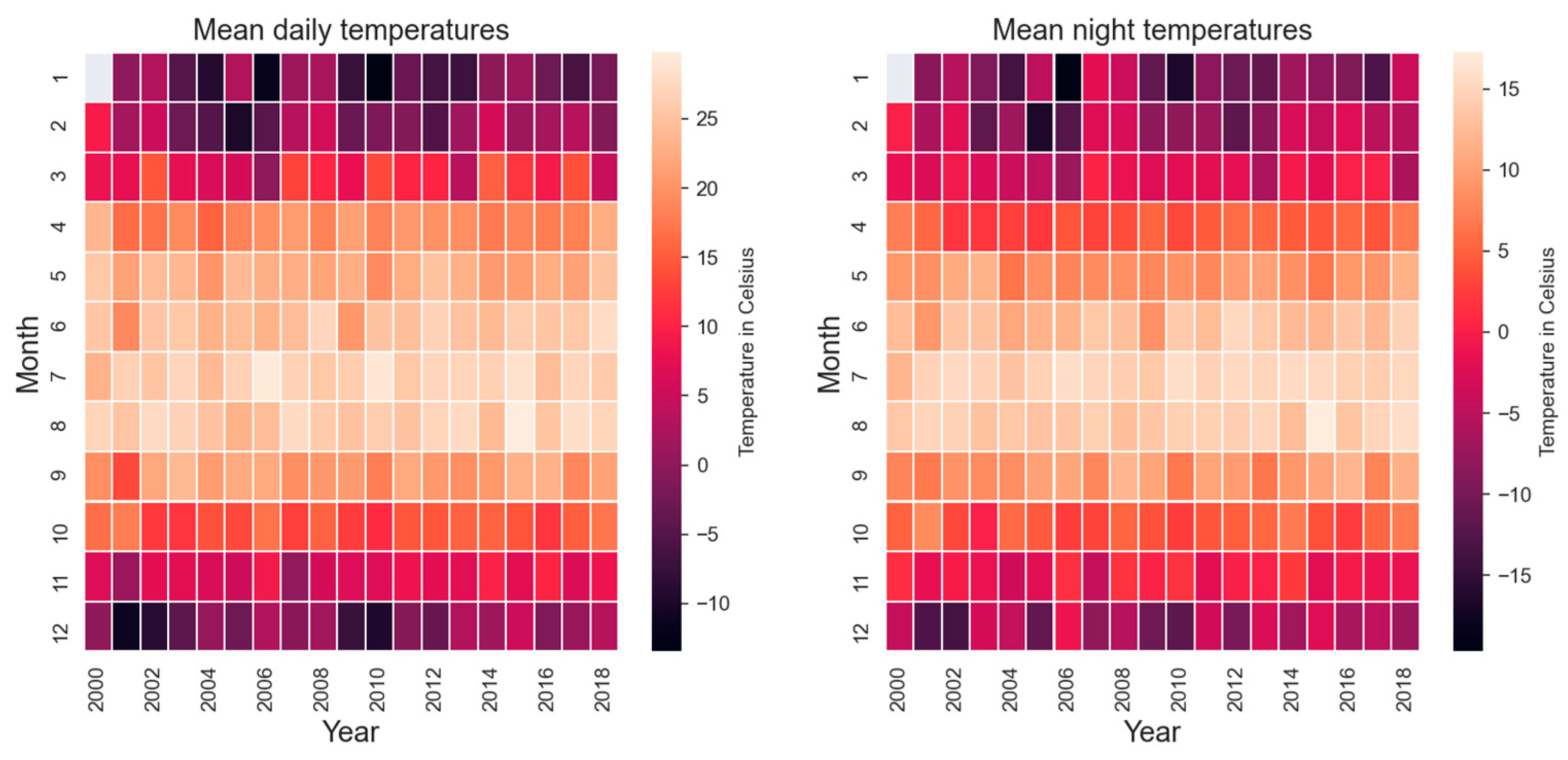
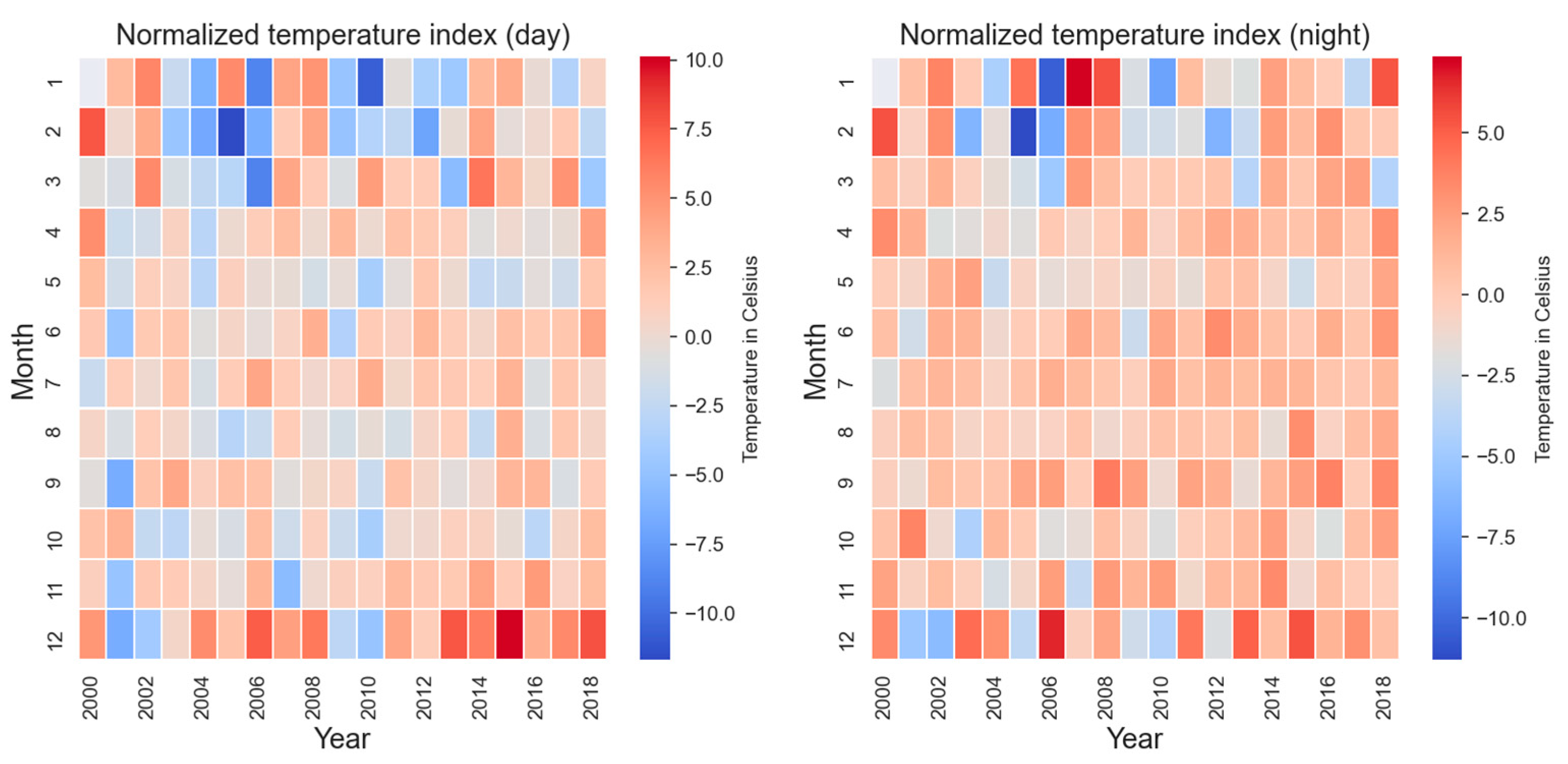
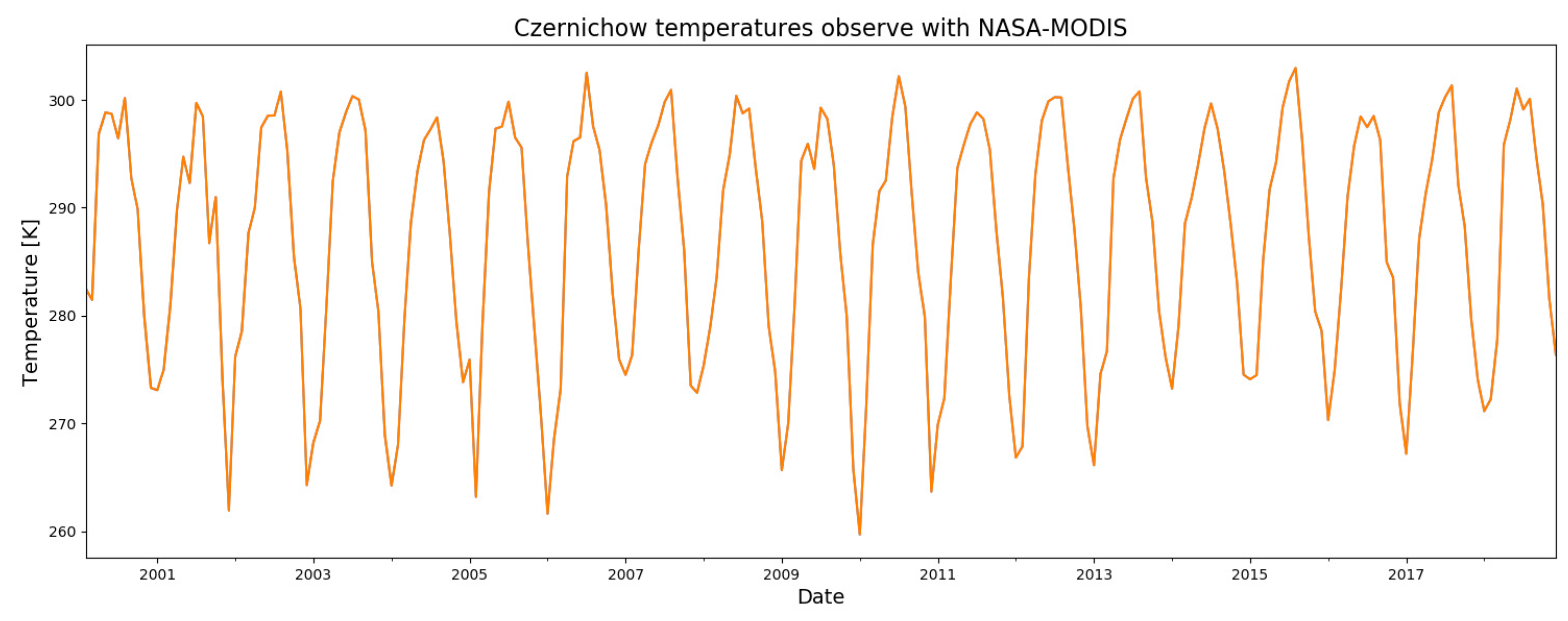
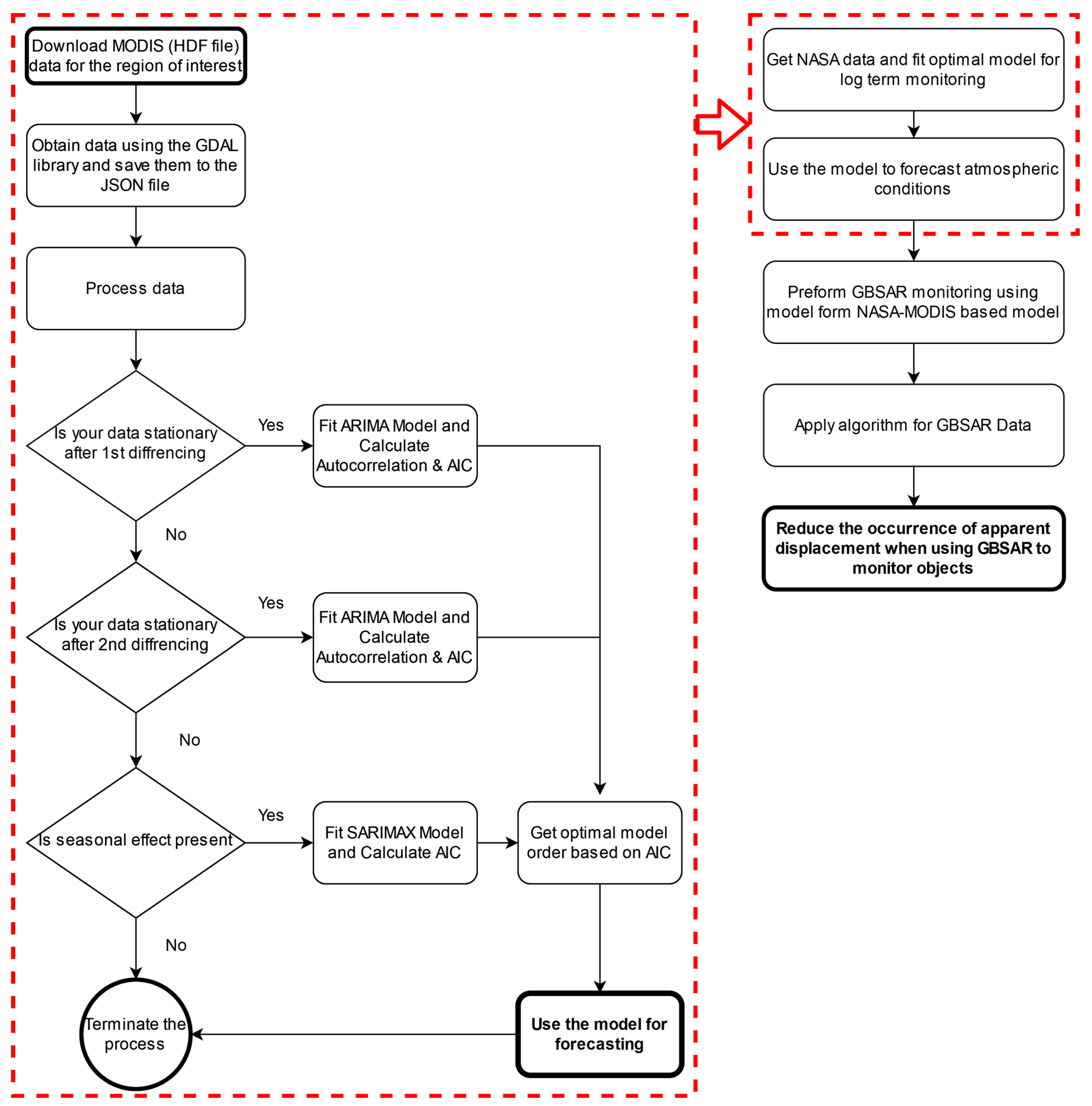
• The MODIS–NASA data are used for the preliminary assessment of weather conditions that may occur in the place of the future GBSAR-based monitoring installation. Such locations rarely have an installation of the weather conditions monitoring established a priori. Therefore, at an early stage of observation (before the weather monitoring station installed together with the GBSAR radar gathers enough data), the model based on MODIS data is valuable.
• The data model used is SARIMAX due to seasonal effects in the data (annual-monthly for MODIS data and daily-hourly for GBSAR data)
• After the monitoring process begins, GBSAR radar data and data from the weather monitoring station near the radar installation are collected.
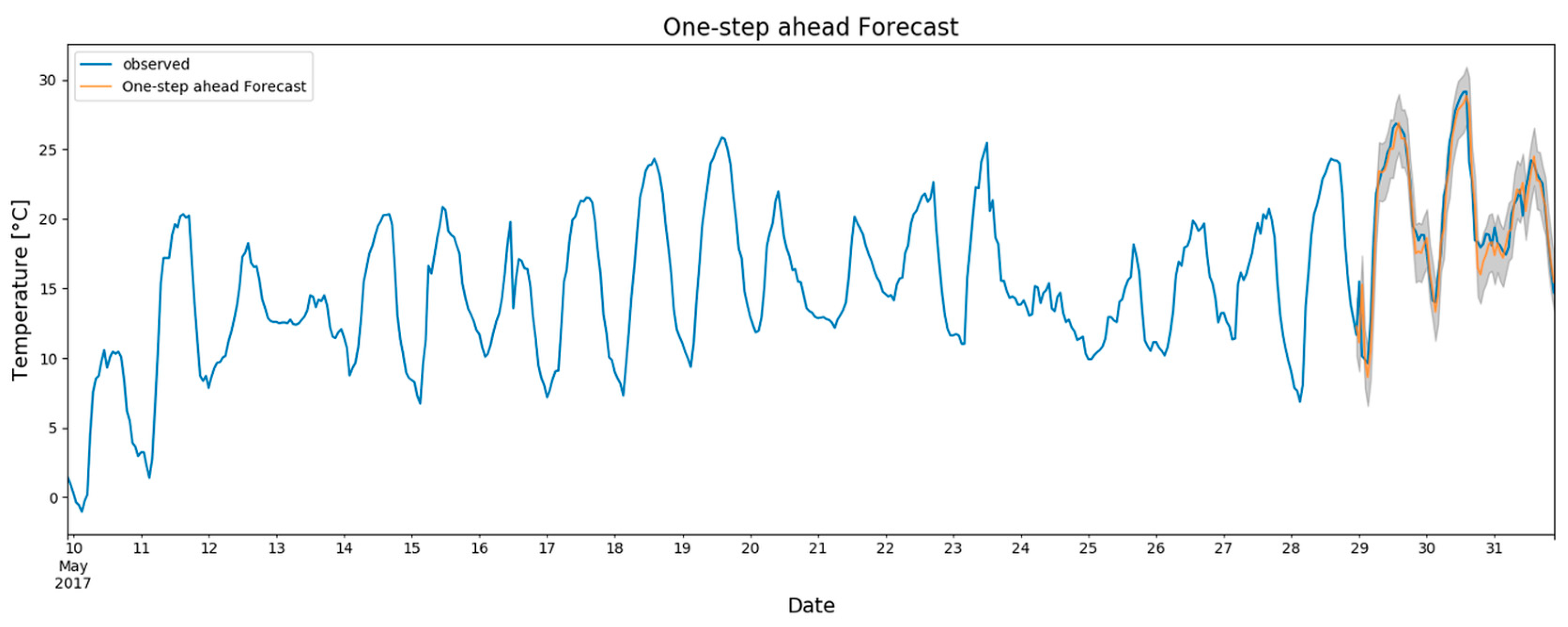
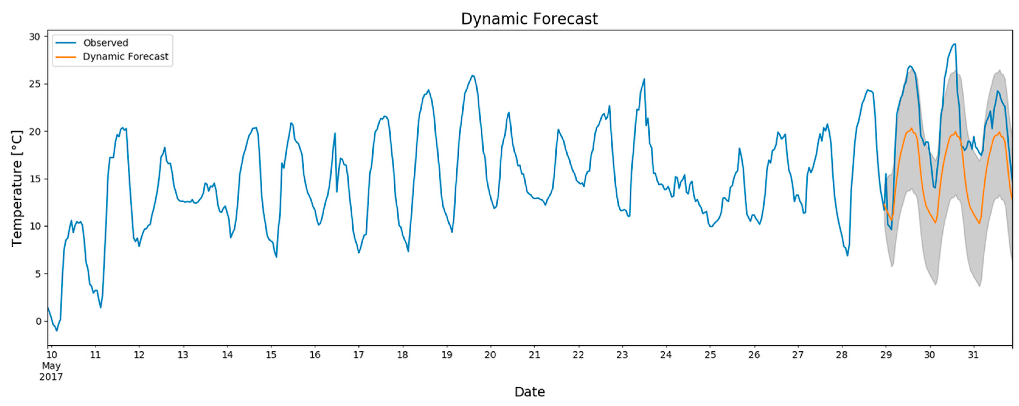
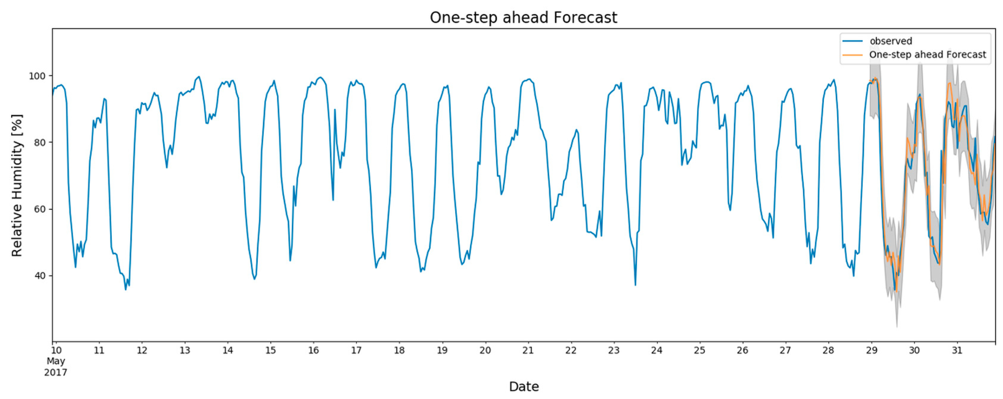
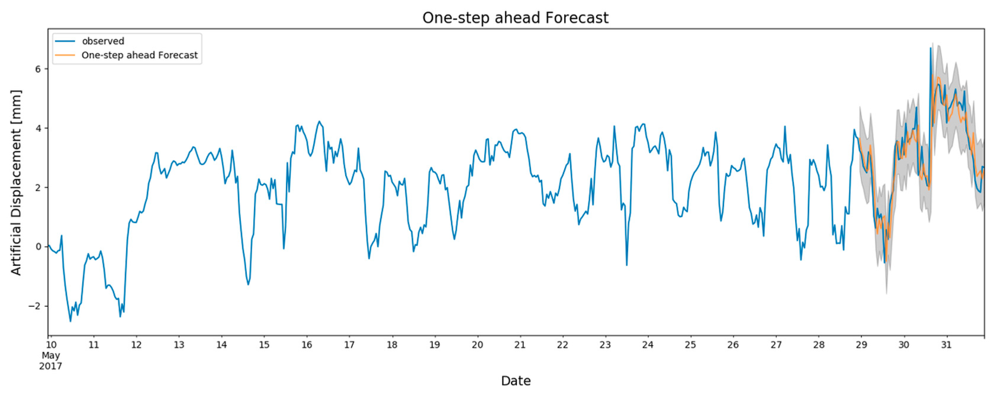
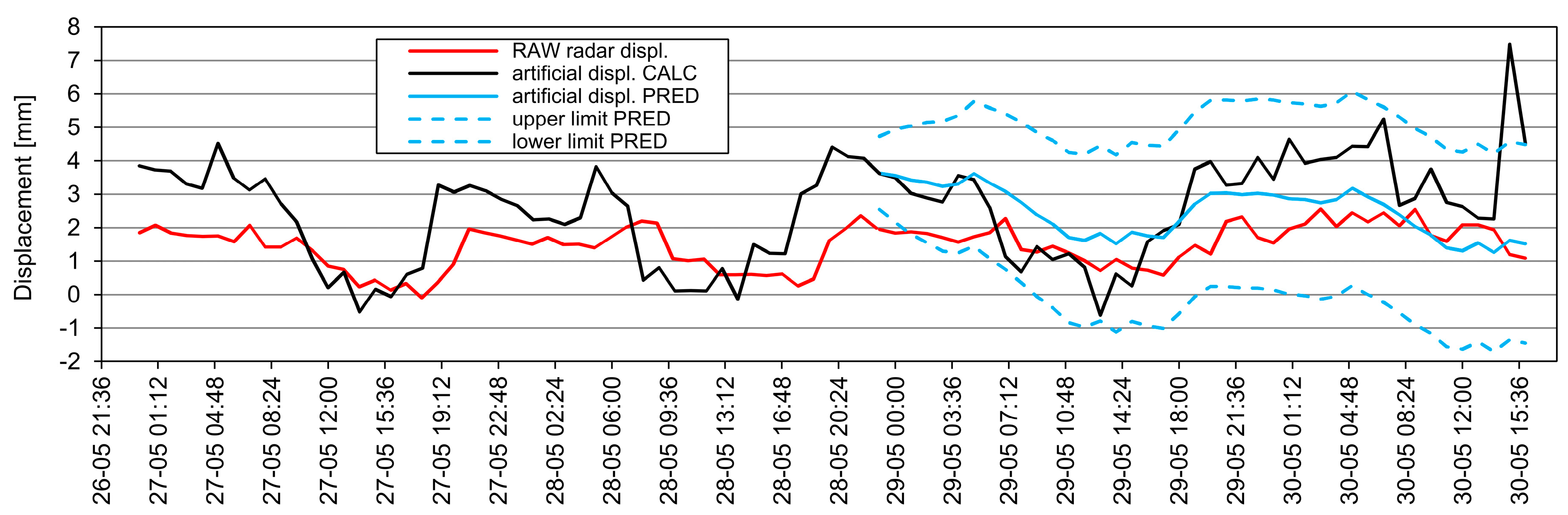
• Data obtained from weather stations for GBSAR observations are modeled as a time series and one-step-ahead prediction is performed on them. Thus, the actual reduction of false alarms is performed on real monitoring data.
• Effective modeling of time series for satellite data allows for partial limitation of false alarms at the initial stage using MODIS–NASA data and for significant limitation of false alarms already at the stage of GBSAR installation working for some time. The proposed algorithm is advantageous because solutions based on so-called stable pixels are practically difficult to implement. It is necessary to have an independent method to check the stability of such a point or assume that selected element of the observed 3D scene is permanent (difficult assumption).
• It should be emphasized that the analysis of the time series in the proposed solution takes place in two blocks of solutions:
  • For the first time for satellite data (assumed that only such data are available for a random location) we obtain an approximate reduction of the problem of false alarms.
  • For the second time based on data collected on site with the most accurate one-step-ahead modeling possible (modeling for each measuring epoch).

The chosen models for data prediction were based on real observations of temperature, pressure and humidity, which were used to calculate the apparent displacements. The goal of the analysis was to determine the period of registered displacement using monitoring systems that should not be interpreted as real displacements for studied objects. Such forecasting allows the prediction of displacement values as caused by changes in atmospheric conditions, even when such data are not available, such as due to system failures. The effectiveness of the apparent displacement forecasting based on varying data coming from observations over different months and seasons is worthy of further examination in subsequent studies.

Two models were examined in this work: static and dynamic. The static model can be treated as a specific case of the dynamic approach where only the nearest value is predicted. Each subsequent value in the static model is based on a real observation. Forecasting using the static model is more accurate than the dynamic approach, which becomes increasingly less accurate with each step. Further studies on this topic should address for how long the forecasting period gives credible results. This will enable estimating the required intermittency of the atmospheric data so as not to significantly influence their interpretation as physical object displacements.

It is noted that even relatively simple estimation models for the time series gave valuable results. Based on the AIC criteria, the authors illustrated the practical usefulness of models with an order of 2 or less. The results show that the classic method of machine learning characteristic for a low calculation complexity can successfully lower the risk of false alarms in GBSAR monitoring.

5. Conclusions

This work presents an effective approach of using publicly accessible NASA–MODIS satellite data to reduce the occurrence of apparent displacements when using GBSAR to monitor objects. The authors demonstrate an effective application of the time series analyses for both the respective components of the atmospheric state (pressure, temperature and humidity), as well as the phenomenon of apparent displacements. The presented technique is universal and can be applied to current and future projects related to deformation studies. The model order effectively achieved through calculations is not overestimated; therefore, it does not add significant calculation complexity to the results.

References

1. Tarchi, D.; Rudolf, H.; Luzi, G.; Chiarantini, L.; Coppo, P.; Sieber, A.J. SAR interferometry for structural changes detection; A demonstration test on a dam. Proc. IGARSS IEEE 1999 Int. Geosci. Remote Sens. Symp. IGARSS’99 1999, 3, 1522–1524. [Google Scholar]
2. Pieraccini, M.; Tarchi, D.; Rudolf, H.; Leva, D.; Luzi, G.; Atzeni, C. Interferometric radar for remote monitoring of building deformations. Electron. Lett. 2000, 36, 569–570. [Google Scholar] [CrossRef]
3. Hu, C.; Wang, J.Y.; Tian, W.M.; Zeng, T.; Wang, R. Design and Imaging of Ground-Based Multiple-Input Multiple-Output Synthetic Aperture Radar (MIMO SAR) with Non-Collinear Arrays. Sensors 2017, 17, 598. [Google Scholar] [CrossRef] [PubMed]
4. Miller, P.K.; Vessely, M.; Olson, L.D.; Tinkey, Y. Slope stability and rock-fall monitoring with a remote interferometric radar system. In Geo-Congress 2013: Stability and Performance of Slopes and Embankments III; Meehan, C., Pradel, D., Pando, M.A., Labuz, J.F., Eds.; ASCE: San Diego, CA, USA, 2013; pp. 304–318. [Google Scholar]
5. Mazzanti, P.; Bozzano, F.; Cipriani, I.; Prestininzi, A. New insights into the temporal prediction of landslides by a terrestrial SAR interferometry monitoring case study. Landslides 2015, 12, 55–68. [Google Scholar] [CrossRef] [Green Version]
6. Pieraccini, M.; Mecatti, D.; Noferini, L.; Luzi, G.; Franchioni, G.; Atzeni, C. SAR interferometry for detecting the effects of earthquakes on buildings. NDT Int. 2002, 35, 615–625. [Google Scholar] [CrossRef]
7. Dematteis, N.; Luzi, G.; Giordan, D.; Zucca, F.; Allasia, P. Monitoring Alpine glacier surface deformations with GB-SAR. Remote Sens. Lett. 2017, 8, 947–956. [Google Scholar] [CrossRef]
8. Luzi, G.; Noferini, L.; Mecatti, D.; Macaluso, G.; Pierracini, M.; Atzeni, C. Using a groundbased SAR interferometer and a terrestrial laser scanner to monitor a snow-covered slope: Results from an experimental data collection in Tyrol (Austria). IEEE Trans. Geosci. Remote. Sens. 2009, 47, 382–393. [Google Scholar] [CrossRef]
9. Monserrat, O.H.; Crosetto, M.; Luzi, G. A review of ground-based SAR interferometry for deformation measurement. ISPRS J. Photogramm. Remote. Sens. 2014, 93, 40–48. [Google Scholar] [CrossRef] [Green Version]
10. Huang, Z.; Sun, J.; Li, Q.; Tan, W.; Huang, P.; Qi, Y. Time- and Space-Varying Atmospheric Phase Correction in Discontinuous Ground-Based Synthetic Aperture Radar Deformation Monitoring. Sensors 2018, 18, 3883. [Google Scholar] [CrossRef] [PubMed] [Green Version]
11. Wang, Z.; Li, Z.; Mills, J. Modelling of instrument repositioning errors in discontinuous Multi-Campaign Ground-Based SAR (MC-GBSAR) deformation monitoring. ISPRS J. Photogramm. Remote Sens. 2019, 157, 26–40. [Google Scholar] [CrossRef]
12. Zebker, H.A.; Rosen, P.A.; Hensley, S. Atmospheric effects in interferometric synthetic aperture radar surface deformation and topographic maps. J. Geophys. Res. Solid Earth 1997, 102, 7547–7563. [Google Scholar] [CrossRef]
13. Leva, D.; Nico, G.; Tarchi, D.; Fortuny-Guasch, J.; Sieber, A.J. Temporal analysis of a landslide by means of a ground-based SAR interferometer IEEE Trans. Geosci. Remote. Sens. 2003, 41, 745–752. [Google Scholar] [CrossRef]
14. Noferini, L.; Pieraccini, M.; Mecatti, D.; Luzi, G.; Atzeni, C.; Tamburini, A.; Broccolato, M. Permanent scatterers analysis for atmospheric correction in ground-based SAR interferometry IEEE Trans. Geosci. Remote Sens. 2005, 43, 1459–1471. [Google Scholar] [CrossRef]
15. Iannini, L.; Guarnieri, A.M. Atmospheric phase screen in groundbased radar: Statistics and compensation. IEEE Geosci. Remote Sens. Lett. 2011, 8, 537–541. [Google Scholar] [CrossRef] [Green Version]
16. Iglesias, R.; Fabregas, X.; Aguasca, A.; Mallorqui, J.J.; López-Martínez, C.; Gili, J.A.; Corominas, J.A. Atmospheric Phase Screen Compensation in Ground-Based SAR With a Multiple-Regression Model Over Mountainous Regions. IEEE Trans. Geosci. Remote Sens. 2014, 52, 2436–2449. [Google Scholar] [CrossRef]
17. Wan, Z.; Hook, S.; Hulley, G. MOD11B3 MODIS/Terra Land Surface Temperature/Emissivity Monthly L3 Global 6 km SIN Grid V006; NASA EOSDIS LP DAAC: Sioux Falls, SD, USA, 2015.
18. Stanisz, J.; Borecka, A.; Pilecki, Z.; Kaczmarczyk, R. Numerical simulation of pore pressure changes in levee under flood conditions. In E3S Web of Conferences; EDP Sciences: Les Ulis, France, 2017; Volume 24, p. 03002. [Google Scholar]
19. Gentile, C.; Bernardini, G. An interferometric radar for non-contact measurement of deflections on civil engineering structures: Laboratory and full-scale tests. Struct. Infrastruct. Eng. 2010, 6, 521–534. [Google Scholar] [CrossRef]
20. Bozzano, F.; Cipriani, I.; Mazzanti, P.; Prestininzi, A. Displacement patterns of a landslide affected by human activities: Insights from ground-based InSAR monitoring. Nat. Hazards 2011, 59, 1377–1396. [Google Scholar] [CrossRef]
21. Xing, C.; Yu, Z.Q.; Zhou, X.; Wang, P. Research on the Testing Methods for IBIS-S System. In IOP Conference Series: Earth and Environmental Science; IOP Publishing: Bristol, UK, 2014; Volume 17, p. 012263. [Google Scholar]
22. Durbin, J.; Siem, J.K. Time Series Analysis by State Space Methods, 2nd ed.; Oxford University Press: Oxford, UK, 2012. [Google Scholar]
23. Luzi, G.; Pieraccini, M.; Mecatti, D.; Noferini, L.; Guidi, G.; Moia, F.; Atzeni, C. Ground-Based Interferometry for Landslides Monitoring: Atmospheric and Instrumental Decorrelation Sources on Experimental Data. IEEE Trans. Geosci. Remote Sens. 2004, 42, 2454–2466. [Google Scholar] [CrossRef]
24. Smith, K.; Weintraub, S. The Constants in the Equation for Atmospheric Refractive Index at Radio Frequencies. Proc. IRE IEEE 1953, 41, 1035–1037. [Google Scholar] [CrossRef] [Green Version]
25. Kraus, H. Die Atmosphaere der Erde: Eine Einfuehrung in Meteorologie; Springer: Berlin, Germany, 2004. [Google Scholar]
Figure 1. Example of a moderate resolution imaging spectroradiometer (MODIS) scene from the middle-east region in Europe. Pixel ground size is 6 km.
Remotesensing 12 02236 g001
Figure 2. Experimental flood embankment as the subject of ground-based radar interferometry (GBSAR) observations.
Remotesensing 12 02236 g002
Figure 3. Image by interferometric survey—landslide (IBIS-L) radar installation site.
Remotesensing 12 02236 g003
Figure 4. Raw radar observations of the displacements for three selected points (no. 9, 14, 19) on the embankment.
Remotesensing 12 02236 g004
Figure 5. Mean daily and nightly temperatures for Czernichow.
Remotesensing 12 02236 g005
Figure 6. Normalized temperature index (day and night) from 2000–2018.
Remotesensing 12 02236 g006
Figure 7. Original data series along with first and second differencing with autocorrelation. The time unit for x-axis is the number of months since the first data acquisition. Final-day temperature of each month is represented.
Remotesensing 12 02236 g007
Figure 8. Original data series. Temperature (given in Kelvin) observed in 2000–2018 period by NASA–MODIS in Czernichow (Poland).
Remotesensing 12 02236 g008
Figure 9. Diagnostic plots for the SARIMAX (1, 1, 1) × (0, 1, 1) 12 model. Top-left shows standardized residuals for SARIMAX, bottom-left presents quantile-quantile plot, top-right gives histogram and normal density plot and bottom-left gives correlogram.
Remotesensing 12 02236 g009
Figure 10. Modeled temperature (2017–2019) along with the measured data.
Remotesensing 12 02236 g010
Figure 11. Raw temperature data series obtained during the IBIS measurements.
Remotesensing 12 02236 g011
Figure 12. Diagnostic plots for the raw temperature data series obtained from IBIS measurements with a SARIMAX (1, 0, 2) × (0, 1, 2) 24 model.
Remotesensing 12 02236 g012
Figure 13. Training data and forecasting results in the static mode for the raw temperature data time series obtained from the IBIS measurements with a SARIMAX (1, 0, 2) × (0, 1, 2) 24 model.
Remotesensing 12 02236 g013
Figure 14. Training data and forecasting result in the dynamic mode for the raw temperature data time series obtained from the IBIS measurements for a SARIMAX (1, 0, 2) × (0, 1, 2) 24 model.
Remotesensing 12 02236 g014
Figure 15. Relative humidity data series calculated from the weather data as obtained during the IBIS measurements.
Remotesensing 12 02236 g015
Figure 16. Diagnostic plots for the relative humidity series obtained during the IBIS measurements for the SARIMAX (1, 0, 1) × (0, 1, 1) 24 model.
Remotesensing 12 02236 g016
Figure 17. Training data and forecasting result for the relative humidity series obtained during the IBIS measurements for the SARIMAX (1, 0, 1) × (0, 1, 1) 24 model.
Remotesensing 12 02236 g017
Figure 18. Apparent displacement data series calculated from the weather data obtained during the IBIS measurements.
Remotesensing 12 02236 g018
Figure 19. Diagnostic plots for the apparent displacement series obtained during the IBIS measurements for the SARIMAX (1, 0, 1) × (0, 1, 1) 24 model.
Remotesensing 12 02236 g019
Figure 20. Training data and forecasted results for the apparent displacement time series obtained during the IBIS measurements for the SARIMAX (1, 0, 1) × (0, 1, 1) 24 model.
Remotesensing 12 02236 g020
Figure 21. Comparison of the raw radar displacements (red), calculated apparent displacements (black) and the predicted apparent displacements (blue).
Remotesensing 12 02236 g021
Figure 22. Complete flowchart of the presented algorithm.
Remotesensing 12 02236 g022