Extreme Gradient Boosting Model for Rain Retrieval using Radar Reflectivity from Various Elevation Angles


Abstract
:
1. Introduction
2. Study Area and Data
2.1. Radar Reflectivity
2.2. Ground Observations
2.3. Dataset Definitions
3. Case Design and Algorithms
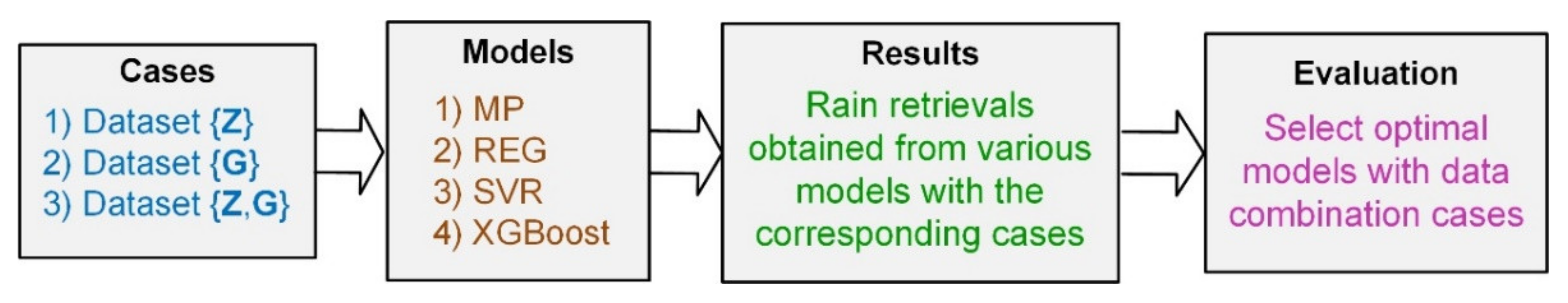
- Case 1 used radar reflectivity {Z} to retrieve rainfall rate. This case used radar reflectivity from every elevation angle as the model input to establish separate models. For example, the radar reflectivity from an elevation angle of 0.5° formulates ML-based rainfall retrieval models (namely subcase 1.1). That is, R = f1(Z1), where f1() can be an ML-based model or the MP formula. Because there were nine elevation angles, nine models were established (i.e., subcases 1.1 to 1.9). An additional model, subcase 1.10, featured a specific model that used radar reflectivity of all elevation angles; that is, R = f2({Zi}i=1,9), where f2() represents using ML-based models.
- Case 2 used meteorological attributes {Gk}k=1,6 of weather stations to retrieve rainfall rate; that is, R = f3({Gk}k=1,6), where f3() represents using ML-based models.
- Case 3 combined reflectivity intensity {Z} and meteorological attributes {G} to retrieve rainfall rate. Nine elevation angles (Z1 to Z9) separately combined with {Gk}k=1,6 can build nine models (i.e., subcases 3.1 to 3.9). For example, for subcase 3.2, R = f4(Z2, {Gk}k=1,6), where f4() represents ML-based models. An additional model, subcase 3.10, featured a specific model that combined meteorological attributes with the radar reflectivity of all elevation angles; that is, R = f5({Zi}i=1,9, {Gk}k=1,6), where f5() represents using ML-based models.
3.1. Algorithms
- 1.
- REG
- 2.
- SVR
- 3.
- XGBoost
3.2. Programming Tools
3.3. Performance Criteria
4. Modeling
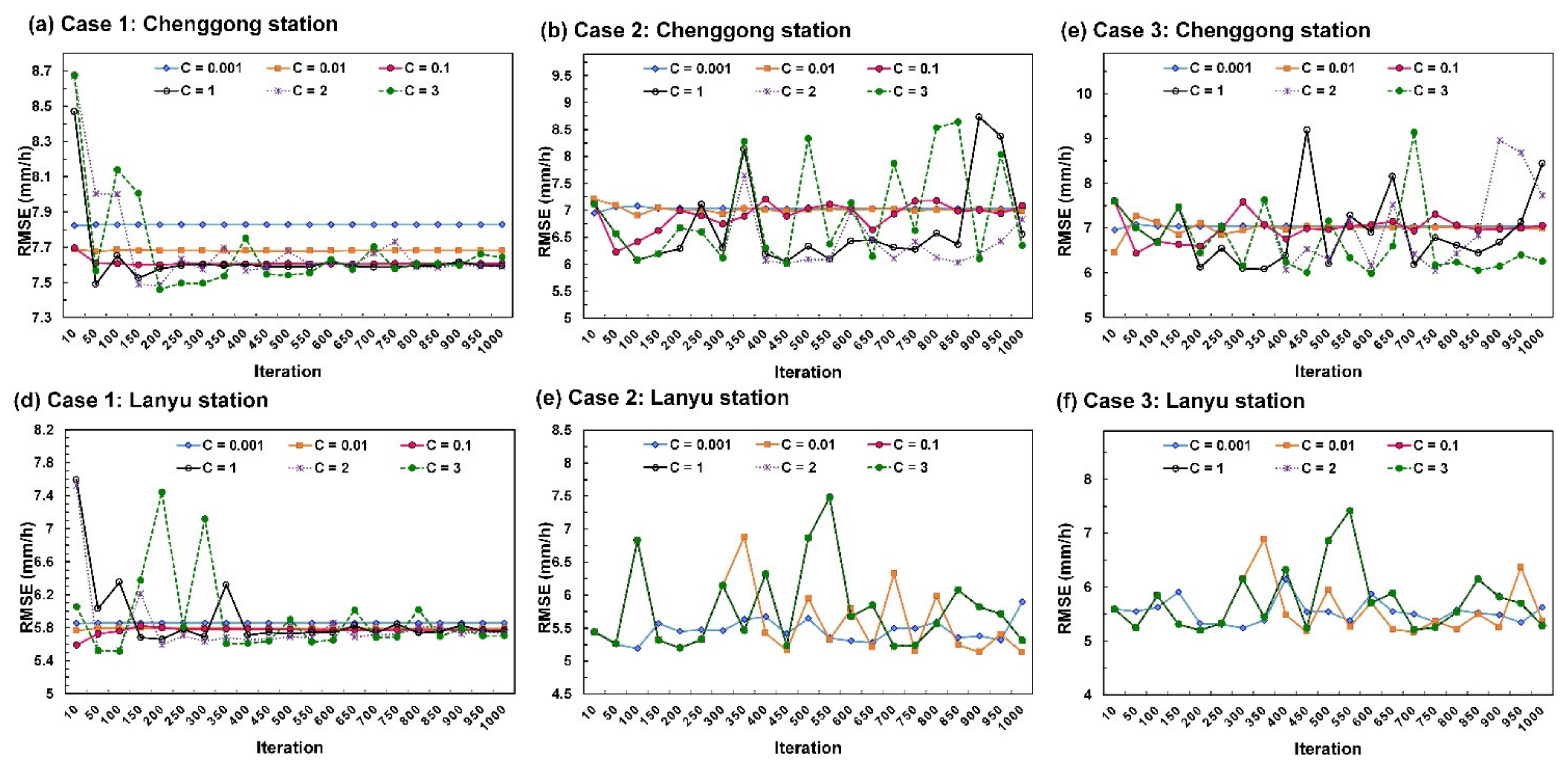
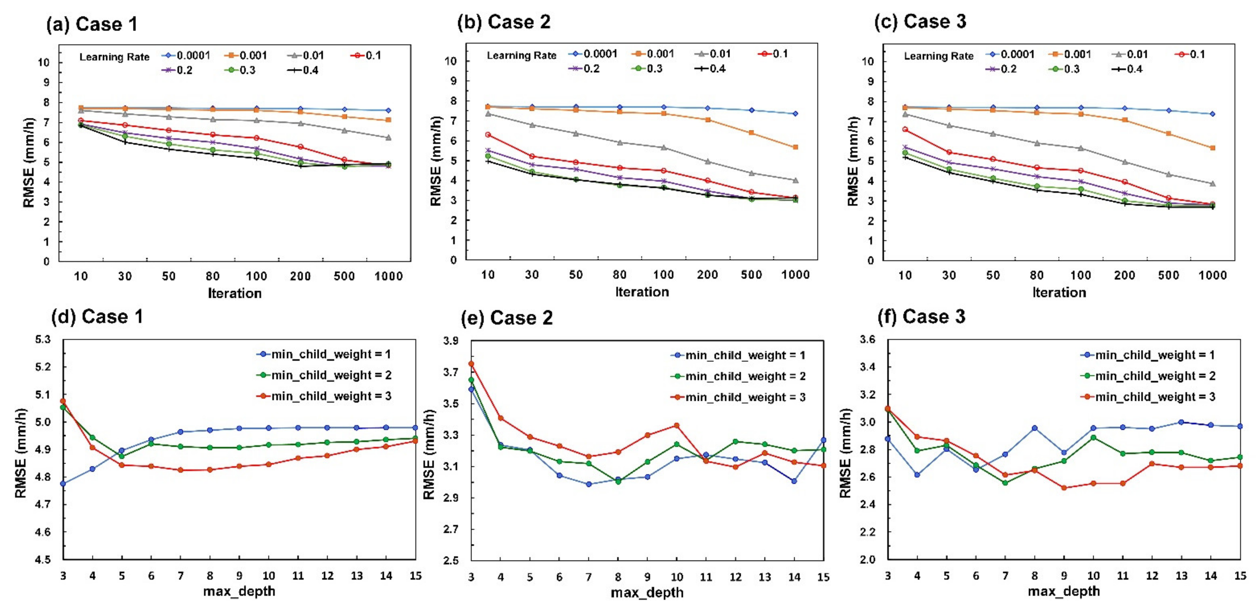
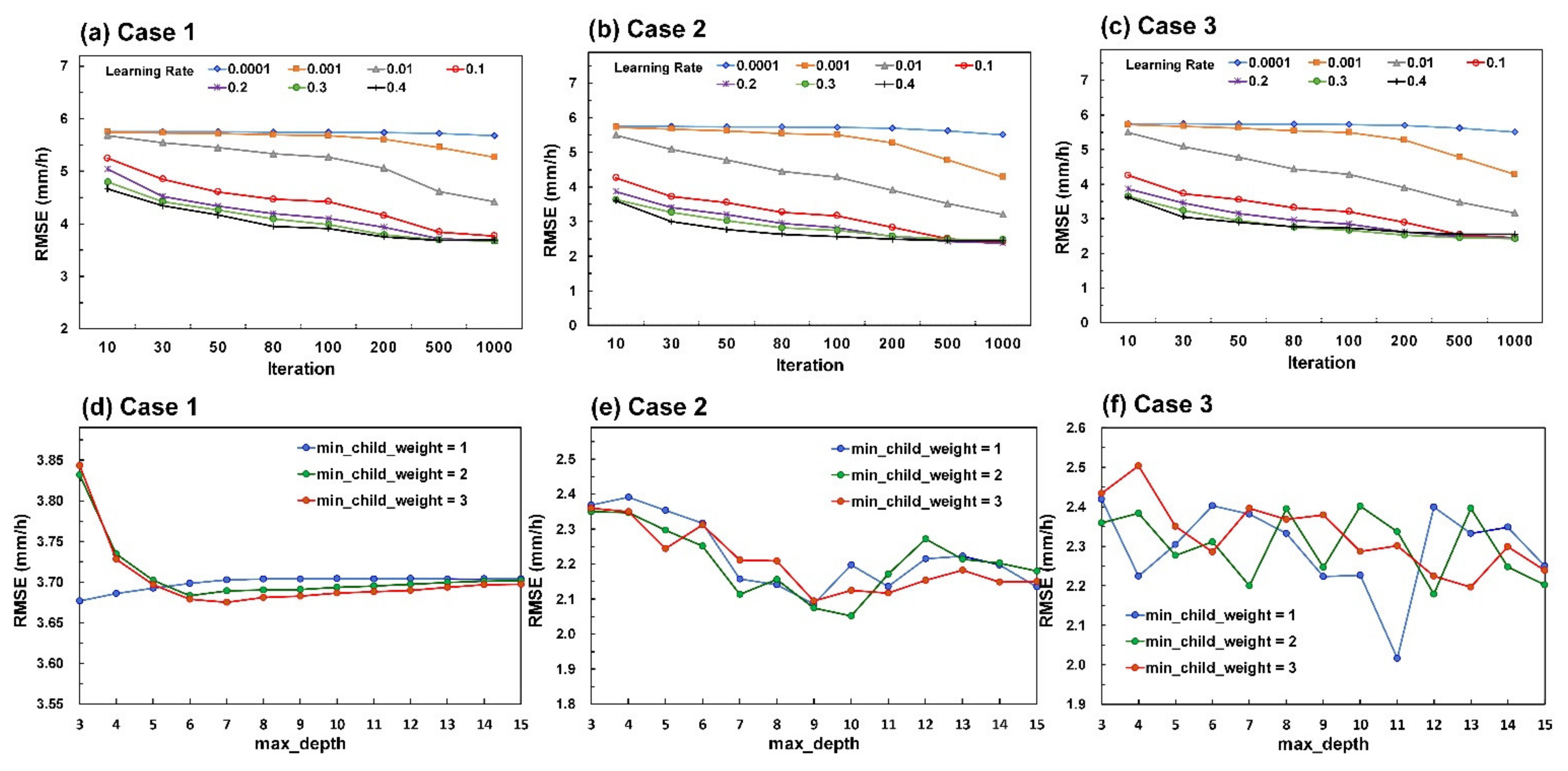
4.1. Parameter Calibration
4.2. Model Performance
5. Evaluation and Discussion
6. Simulations
7. Conclusions
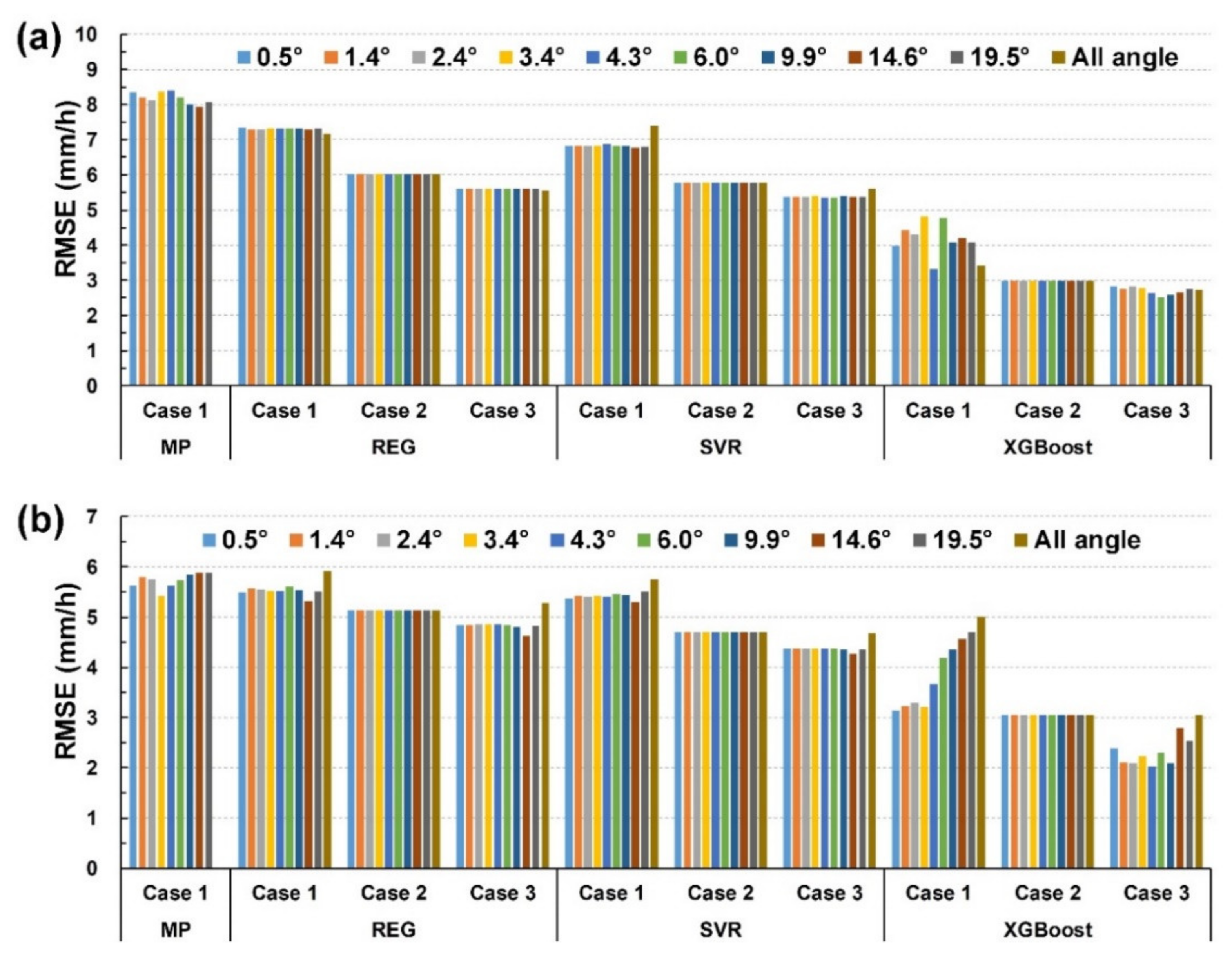
- In the process of building the rainfall-retrieval models, combining radar reflectivity with ground meteorological attributes (Case 3) achieved superior rainfall-retrieval results compared with only inputting radar reflectivity (Case 1) or only ground meteorological attributes (Case 2).
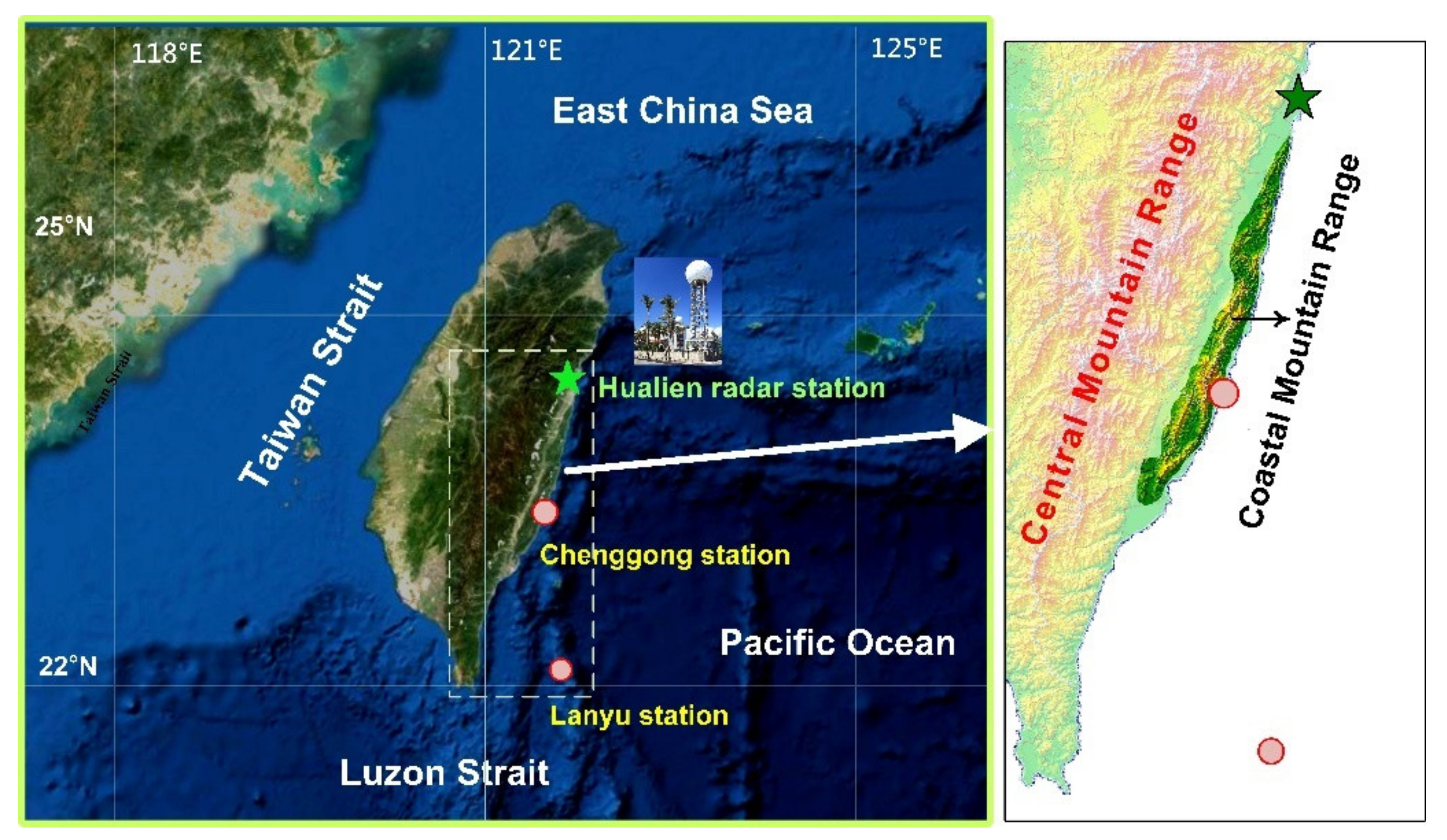
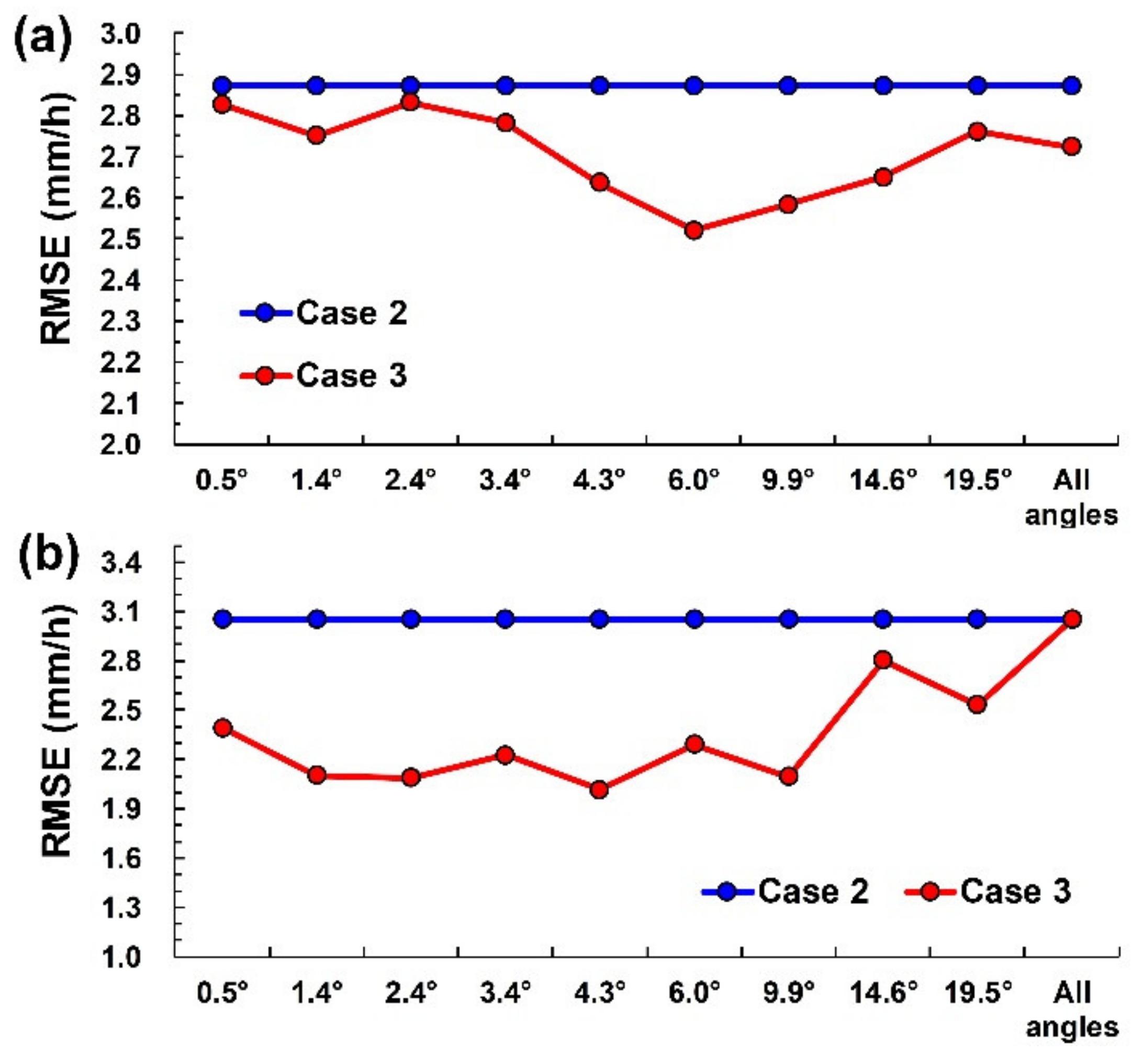
- When the experimental station radar elevation angles were evaluated, radar reflectivity at an elevation angle of 6.0° combined with ground meteorological attributes were the optimal input variables for rainfall retrieval at Chenggong station; at Lanyu station, the optimal input variables were radar reflectivity at an elevation angle of 4.3° combined with ground meteorological attributes.
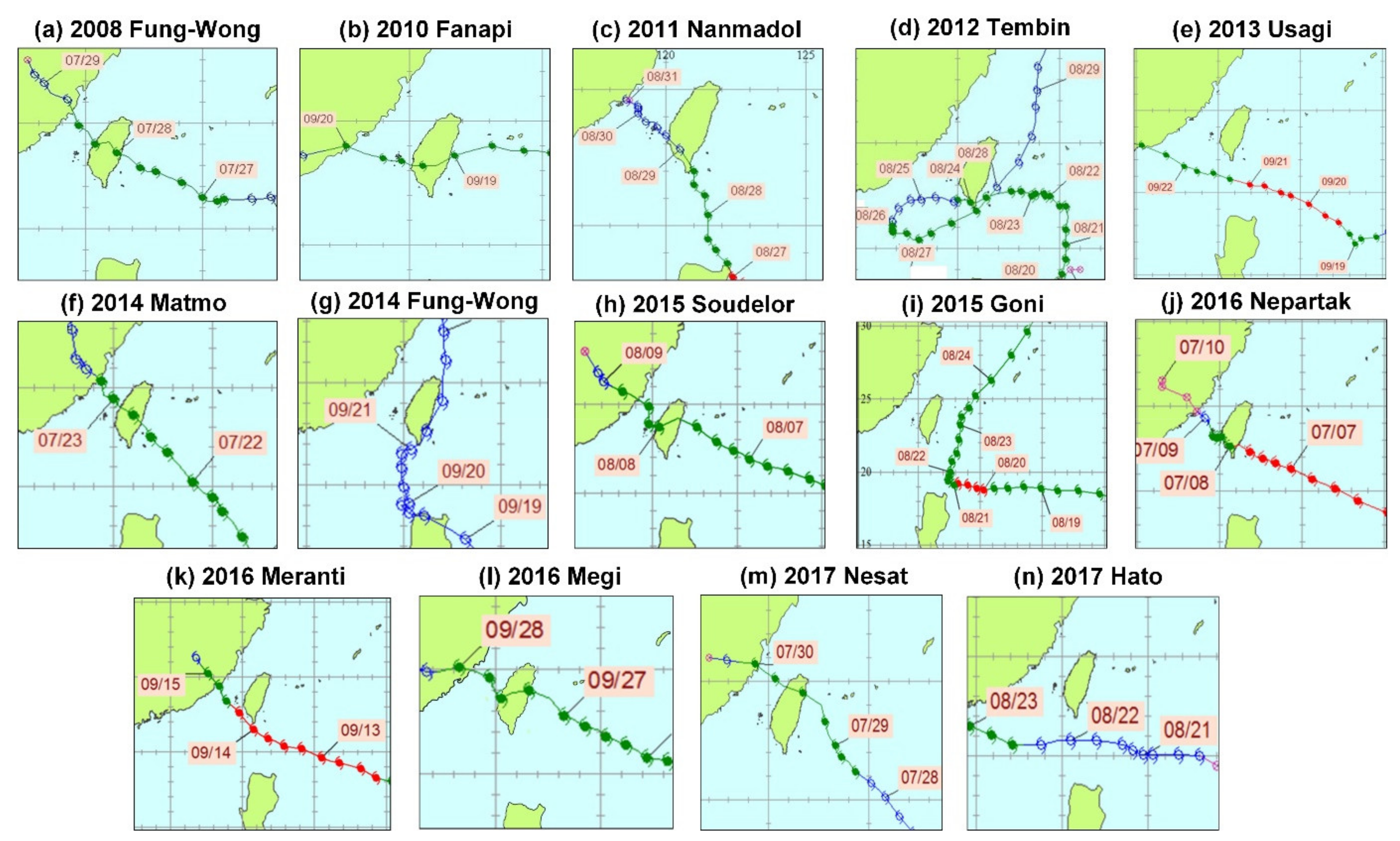
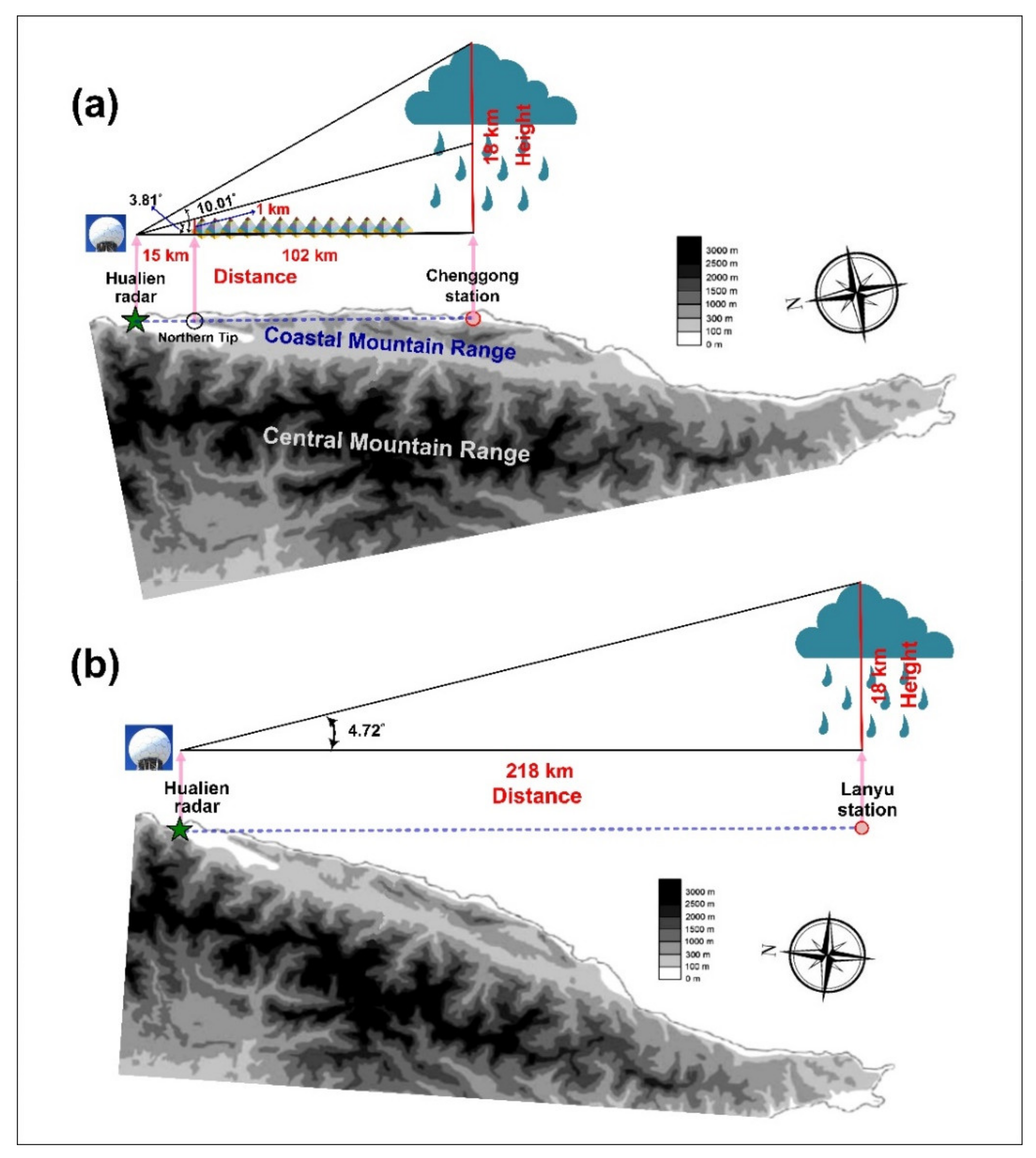
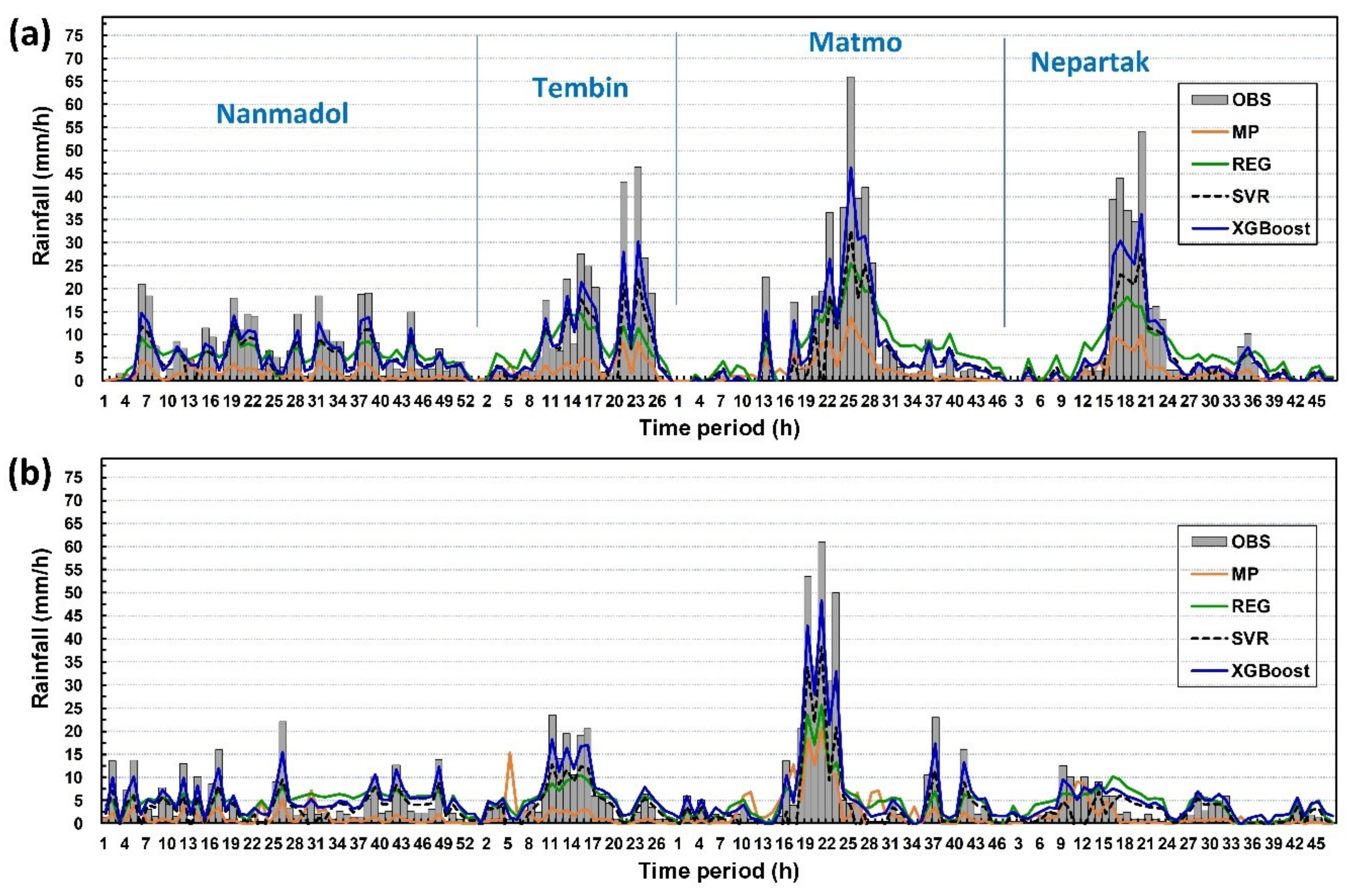
- Simulation results of the testing typhoons (Nanmadol in 2011, Tembin in 2012, Matmo in 2014, and Nepartak in 2016) demonstrated that Lanyu station exhibited smaller error index values in model retrieval than Chenggong station. This study speculated that this is because Lanyu station is situated on the ocean, where a typhoon circulation encounters little to no topographical interference to affect its structure when passing; as a result, the radar reflectivity signals are better reflected off the variations (gradients) of water vapor and possibly rain. By contrast, Chenggong station is affected by rapid changes in typhoon circulation and structure when a typhoon circulation encounters land and the Coastal Mountain Range and the Central Mountain Range, resulting in greater fluctuations in radar reflectivity signals. As a result, the Chenggong station retrieval models were worse at predicting rainfall than those at Lanyu station.
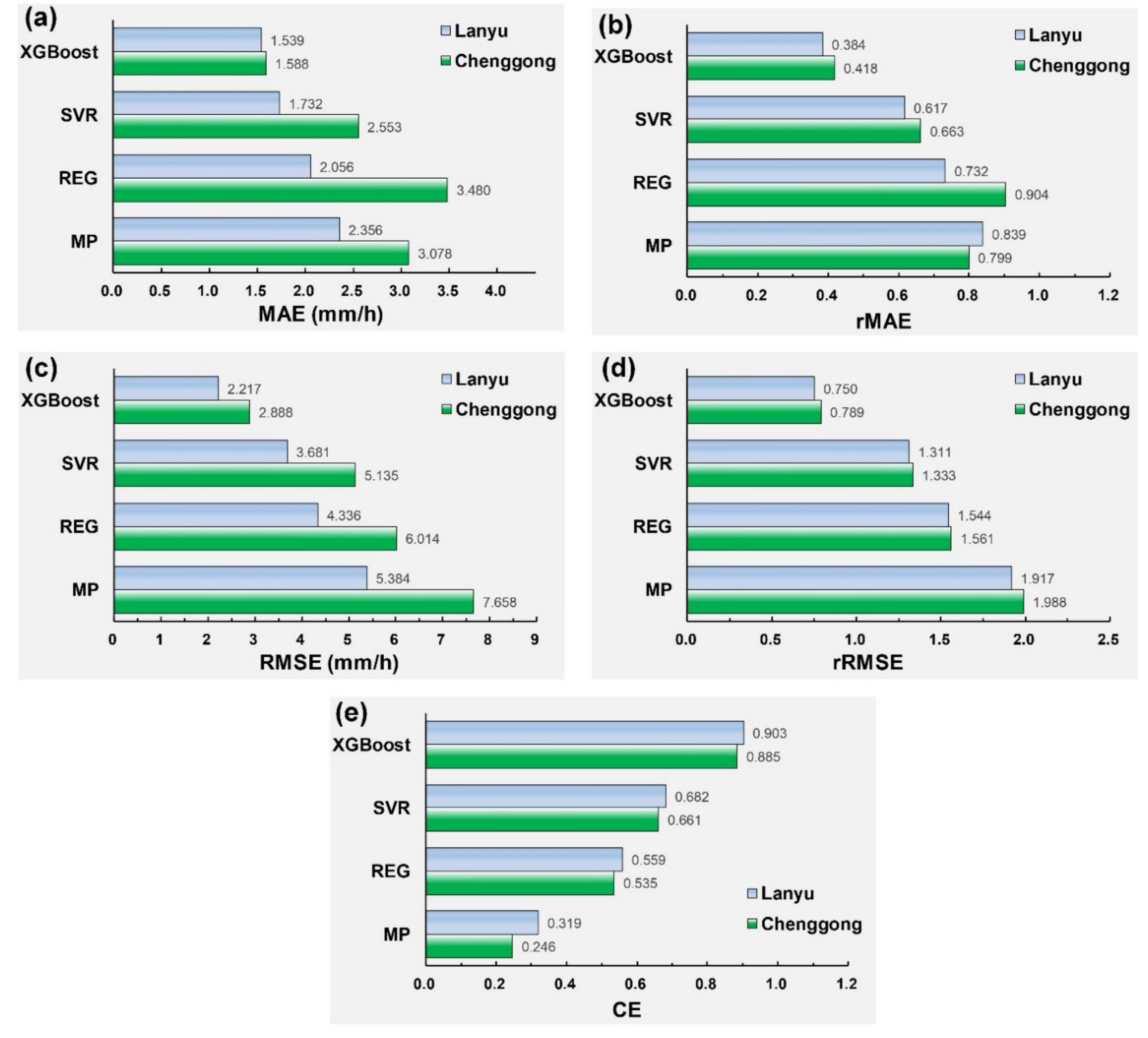
- In terms of model errors, the XGBoost model at both Chenggong and Lanyu stations exhibited smaller error indices than the MP, REG, and SVR models (including absolute errors (MAE and RMSE) and relative errors (rMAE and rRMSE)). In terms of efficiency performance during retrievals, Lanyu station’s XGBoost model had the highest efficiency coefficient (0.903), and Chenggong station’s XGBoost model had the second highest (0.885).
Author Contributions
Funding
Acknowledgments
Conflicts of Interest
References
- Roy, C.; Kovordányi, R. Tropical cyclone track forecasting techniques: A review. Atmos. Res. 2012, 104, 40–69. [Google Scholar] [CrossRef] [Green Version]
- Wei, C.C. Improvement of typhoon precipitation forecast efficiency by coupling SSM/I microwave data with climatologic characteristics and precipitation. Weather Forecast. 2013, 28, 614–630. [Google Scholar] [CrossRef]
- Huang, J.C.; Yu, C.K.; Lee, J.Y.; Cheng, L.W.; Lee, T.Y.; Kao, S.J. Linking typhoon tracks and spatial rainfall patterns for improving flood lead time predictions over a mesoscale mountainous watershed. Water Resour. Res. 2012, 48, W09540. [Google Scholar] [CrossRef]
- Kuo, Y.C.; Lee, M.A.; Lu, M.M. Association of Taiwan’s October rainfall patterns with large-scale oceanic and atmospheric phenomena. Atmos. Res. 2016, 180, 200–210. [Google Scholar] [CrossRef]
- Wei, C.C.; Peng, P.C.; Tsai, C.H.; Huang, C.L. Regional forecasting of wind speeds during typhoon landfall in Taiwan: A case study of westward-moving typhoons. Atmosphere 2018, 9, 141. [Google Scholar] [CrossRef] [Green Version]
- Chen, K.S.; Wang, J.T.; Mitnik, L.M. Satellite and ground observations of the evolution of Typhoon Herb near Taiwan. Remote Sens. Environ. 2001, 75, 397–411. [Google Scholar] [CrossRef]
- Wei, C.C.; Roan, J. Retrievals for the rainfall rate over land using Special Sensor Microwave/Imager data during tropical cyclones: Comparisons of scattering index, regression, and support vector regression. J. Hydrometeorol. 2012, 13, 1567–1578. [Google Scholar] [CrossRef]
- Zhang, Y.; Stensrud, D.J.; Zhang, F. Simultaneous assimilation of radar and all-sky satellite infrared radiance observations for convection-allowing ensemble analysis and prediction of severe thunderstorms. Mon. Weather Rev. 2019, 147, 4389–4409. [Google Scholar] [CrossRef]
- Marshall, J.S.; Palmer, W.M.K. The distribution of raindrops with size. J. Appl. Meteorol. 1948, 5, 165–166. [Google Scholar] [CrossRef]
- Scofield, R.A.; Kuligowski, R.J. Status and outlook of operational satellite precipitation algorithms for extreme-precipitation events. Weather Forecast. 2003, 18, 1037–1051. [Google Scholar] [CrossRef] [Green Version]
- Smith, J.A.; Baeck, M.L.; Meierdiercks, K.L.; Miller, A.J.; Krajewski, W.F. Radar rainfall estimation for flash flood forecasting in small urban watersheds. Adv. Water Resour. 2007, 30, 2087–2097. [Google Scholar] [CrossRef]
- Michaelides, S.; Levizzani, V.; Anagnostou, E.; Bauer, P.; Kasparis, T.; Lane, J.E. Precipitation: Measurement, remote sensing, climatology and modeling. Atmos. Res. 2009, 94, 512–533. [Google Scholar] [CrossRef]
- Wei, C.C. Wavelet support vector machines for forecasting precipitation in tropical cyclones: Comparisons with GSVM, regression, and MM5. Weather Forecast. 2012, 27, 438–450. [Google Scholar] [CrossRef]
- Diop, C.A.; Sauvageot, H.; Mesnard, F. Partitioning the distribution function of radar reflectivity in convective storms using maximum likelihood method. Atmos. Res. 2013, 124, 123–136. [Google Scholar] [CrossRef]
- Ku, J.M.; Yoo, C. Calibrating radar data in an orographic setting: A case study for the typhoon Nakri in the Hallasan Mountain, Korea. Atmosphere 2017, 8, 250. [Google Scholar] [CrossRef] [Green Version]
- Woo, W.C.; Wong, W.K. Operational application of optical flow techniques to radar-based rainfall nowcasting. Atmosphere 2017, 8, 48. [Google Scholar] [CrossRef] [Green Version]
- Wei, C.C.; Hsieh, P.Y. Estimation of hourly rainfall during typhoons using radar mosaic-based convolutional neural networks. Remote Sens. 2020, 12, 896. [Google Scholar] [CrossRef] [Green Version]
- Borga, M.; Anagnostou, E.N.; Frank, E. On the use of real-time radar rainfall estimates for flood prediction in mountainous basins. J. Geophys. Res. 2000, 105, 2269–2280. [Google Scholar] [CrossRef]
- Gabella, M.; Joss, J.; Perona, G.; Galli, G. Accuracy of rainfall estimates by two radars in the same Alpine environment using gage adjustment. J. Geophys. Res. 2001, 106, 5139–5150. [Google Scholar] [CrossRef] [Green Version]
- Seo, D.J.; Breidenbach, J.P. Real-time correction of spatially nonuniform bias in radar rainfall data using rain gauge measurements. J. Hydrometeorol. 2002, 3, 93–111. [Google Scholar] [CrossRef] [Green Version]
- Libertino, A.; Allamano, P.; Claps, P.; Cremonini, R.; Laio, F. Radar estimation of intense rainfall rates through adaptive calibration of the Z-R relation. Atmosphere 2015, 6, 1559–1577. [Google Scholar] [CrossRef] [Green Version]
- Tang, J.; Matyas, C. A nowcasting model for tropical cyclone precipitation regions based on the TREC motion vector retrieval with a semi-Lagrangian scheme for Doppler weather radar. Atmosphere 2018, 9, 200. [Google Scholar] [CrossRef] [Green Version]
- Chen, Y.; Duan, J.; An, J.; Liu, H. Raindrop size distribution characteristics for tropical cyclones and meiyu-baiu fronts impacting Tokyo, Japan. Atmosphere 2019, 10, 391. [Google Scholar] [CrossRef] [Green Version]
- Asklany, S.A.; Elhelow, I.K.; El-Wahab, M.A. Rainfall events prediction using rule-based fuzzy inference system. Atmos. Res. 2011, 101, 228–236. [Google Scholar] [CrossRef]
- Wei, C.C. RBF neural networks combined with principal component analysis applied to quantitative precipitation forecast for a reservoir watershed during typhoon periods. J. Hydrometeorol. 2012, 13, 722–734. [Google Scholar] [CrossRef]
- Schmidhuber, J. Deep learning in neural networks: An overview. Neural Netw. 2015, 61, 85–117. [Google Scholar] [CrossRef] [Green Version]
- Lin, F.R.; Wu, N.J.; Tsay, T.K. Applications of cluster analysis and pattern recognition for typhoon hourly rainfall forecast. Adv. Meteorol. 2017, 2017, 5019646. [Google Scholar] [CrossRef]
- Leahy, T.P.; Llopis, F.P.; Palmer, M.D.; Robinson, N.H. Using neural networks to correct historical climate observations. J. Atmos. Ocean. Technol. 2018, 35, 2053–2059. [Google Scholar] [CrossRef]
- Mosavi, A.; Ozturk, P.; Chau, K.W. Flood prediction using machine learning models: Literature review. Water 2018, 10, 1536. [Google Scholar] [CrossRef] [Green Version]
- Jin, Q.; Fan, X.; Liu, J.; Xue, Z.; Jian, H. Using eXtreme Gradient BOOSTing to predict changes in tropical cyclone intensity over the Western North Pacific. Atmosphere 2019, 10, 341. [Google Scholar] [CrossRef] [Green Version]
- Wu, C.L.; Chau, K.W.; Fan, C. Prediction of rainfall time series using modular artificial neural networks coupled with data preprocessing techniques. J. Hydrol. 2010, 389, 146–167. [Google Scholar] [CrossRef] [Green Version]
- Chadwick, R.; Grimes, D. An artificial neural network approach to multispectral rainfall estimation over Africa. J. Hydrometeorol. 2012, 13, 913–931. [Google Scholar] [CrossRef]
- Wei, C.C. Soft computing techniques in ensemble precipitation nowcast. Appl. Soft Comput. 2013, 13, 793–805. [Google Scholar] [CrossRef]
- Wu, C.L.; Chau, K.W. Prediction of rainfall time series using modular soft computing methods. Eng. Appl. Artif. Intell. 2013, 26, 997–1007. [Google Scholar] [CrossRef] [Green Version]
- Kühnlein, M.; Appelhans, T.; Thies, B.; Nauß, T. Precipitation estimates from MSG SEVIRI daytime, nighttime, and twilight data with random forests. J. Appl. Meteorol. Climatol. 2014, 53, 2457–2480. [Google Scholar] [CrossRef] [Green Version]
- Wei, C.C.; You, G.J.Y.; Chen, L.; Chou, C.C.; Roan, J. Diagnosing rain occurrences using passive microwave imagery: A comparative study on probabilistic graphical models and “black box” models. J. Atmos. Ocean. Technol. 2015, 32, 1729–1744. [Google Scholar] [CrossRef]
- Lo, D.C.; Wei, C.C.; Tsai, N.P. Parameter automatic calibration approach for neural-network-based cyclonic precipitation forecast models. Water 2015, 7, 3963–3977. [Google Scholar] [CrossRef] [Green Version]
- He, X.; Chaney, N.W.; Schleiss, M.; Sheffield, J. Spatial downscaling of precipitation using adaptable random forests. Water Resour. Res. 2016, 52, 8217–8237. [Google Scholar] [CrossRef]
- Kashiwao, T.; Nakayama, K.; Ando, S.; Ikeda, K.; Lee, M.; Bahadori, A. A neural network-based local rainfall prediction system using meteorological data on the Internet: A case study using data from the Japan Meteorological Agency. Appl. Soft Comput. 2017, 56, 317–330. [Google Scholar] [CrossRef]
- Wei, C.C. Examining El Niño–Southern Oscillation effects in the subtropical zone to forecast long-distance total rainfall from typhoons: A case study in Taiwan. J. Atmos. Ocean. Technol. 2017, 34, 2141–2161. [Google Scholar] [CrossRef]
- Chiang, Y.M.; Chang, F.J.; Jou, B.J.D.; Lin, P.F. Dynamic ANN for precipitation estimation and forecasting from radar observations. J. Hydrol. 2007, 334, 250–261. [Google Scholar] [CrossRef]
- Wei, C.C. Simulation of operational typhoon rainfall nowcasting using radar reflectivity combined with meteorological data. J. Geophys. Res. Atmos. 2014, 119, 6578–6595. [Google Scholar] [CrossRef]
- Chen, T.; Guestrin, C. XGBoost: A Scalable Tree Boosting System. In KDD’16: Proceedings of the 22nd ACM SIGKDD International Conference on Knowledge Discovery and Data Mining, San Francisco, CA, USA, 13–17 August 2016; ACM—Association for Computing Machinery: New York, NY, USA, 2016; pp. 785–794. [Google Scholar]
- Just, A.C.; Carli, M.M.D.; Shtein, A.; Dorman, M.; Lyapustin, A.; Kloog, I. Correcting measurement error in satellite aerosol optical depth with machine learning for modeling PM2.5 in the Northeastern USA. Remote Sens. 2018, 10, 803. [Google Scholar] [CrossRef] [Green Version]
- Joharestani, M.Z.; Cao, C.; Ni, X.; Bashir, B.; Talebiesfandarani, S. PM2.5 prediction based on random forest, XGBoost, and deep learning using multisource remote sensing data. Atmosphere 2019, 10, 373. [Google Scholar] [CrossRef] [Green Version]
- Jia, Y.; Jin, S.; Savi, P.; Gao, Y.; Tang, J.; Chen, Y.; Li, W. GNSS-R soil moisture retrieval based on a XGboost machine learning aided method: Performance and validation. Remote Sens. 2019, 11, 1655. [Google Scholar] [CrossRef] [Green Version]
- Jin, R.; Li, X.; Che, T. A decision tree algorithm for surface soil freeze/thaw classification over China using SSM/I brightness temperature. Remote Sens. Environ. 2009, 113, 2651–2660. [Google Scholar] [CrossRef]
- Yuan, T.; Sun, Z.; Ma, S. Gearbox fault prediction of wind turbines based on a stacking model and change-point detection. Energies 2019, 12, 4224. [Google Scholar] [CrossRef] [Green Version]
- Lee, Y.; Han, D.; Ahn, M.H.; Im, J.; Lee, S.J. Retrieval of total precipitable water from Himawari-8 AHI Data: A comparison of random forest, extreme gradient boosting, and deep neural network. Remote Sens. 2019, 11, 1741. [Google Scholar] [CrossRef] [Green Version]
- Ko, C.M.; Jeong, Y.Y.; Lee, Y.M.; Kim, B.S. The development of a quantitative precipitation forecast correction technique based on machine learning for hydrological applications. Atmosphere 2020, 11, 111. [Google Scholar] [CrossRef] [Green Version]
- Central Weather Bureau (CWB). Meteorological Telemetry Observation: Meteorological Satellite and Weather Radar; Report of Meteorological Satellite Center: Taipei, Taiwan, 2015. [Google Scholar]
- Jou, B.J.D. Application of doppler radar data on quantitative precipitation forecasting. In The Meteorological Research and Development; Technical Report No. MOTC-CWB-95-6M-01 (in Chinese). Taiwan’s Central Weather Bureau: Taipei, Taiwan, 2006. [Google Scholar]
- Taylor, R. Interpretation of the correlation coefficient: A basic review. J. Diagn. Med Sonogr. 1990, 1, 35–39. [Google Scholar] [CrossRef]
- Yan, X.; Zhang, L.; Li, J.; Du, D.; Hou, F. Entropy-based measures of hypnopompic heart rate variability contribute to the automatic prediction of cardiovascular events. Entropy 2020, 22, 241. [Google Scholar] [CrossRef] [Green Version]
- Zhang, Z.; Li, Y.; Jin, S.; Zhang, Z.; Wang, H.; Qi, L.; Zhou, R. Modulation signal recognition based on information entropy and ensemble learning. Entropy 2018, 20, 198. [Google Scholar] [CrossRef] [Green Version]
- Pedregosa, F.; Varoquaux, G.; Gramfort, A.; Michel, V.; Thirion, B.; Grisel, O.; Blondel, M.; Prettenhofer, P.; Weiss, R.; Dubourg, V.; et al. Scikit-learn: Machine learning in Python. J. Mach. Learn. Res. 2011, 12, 2825–2830. [Google Scholar]
- Chollet, F. Keras: Deep Learning Library for Theano and Tensorflow. 2015. Available online: https://keras.io/ (accessed on 1 February 2020).
- Waco, D.E. Temperatures and turbulence at tropopause levels over Hurricane Beulah (1967). Mon. Weather Rev. 1970, 98, 749–755. [Google Scholar] [CrossRef]
- Houze, R.A.; Lee, W.; Bell, M.M. Convective contribution to the genesis of Hurricane Ophelia (2005). Mon. Weather Rev. 2009, 137, 2778–2800. [Google Scholar] [CrossRef]
- Houze, R.A. Clouds in tropical cyclones. Mon. Weather Rev. 2010, 138, 293–344. [Google Scholar] [CrossRef]


| Typhoon | Duration | Rain (mm) | Intensity | Typhoon | Duration | Rain (mm) | Intensity |
|---|---|---|---|---|---|---|---|
| Fung-Wong | 2008/7/27−28 | 173 | Moderate | Soudelor | 2015/8/7−09 | 159 | Moderate |
| Fanapi | 2010/9/19−20 | 273 | Moderate | Goni | 2015/8/21−22 | 140 | Severe |
| Nanmadol | 2011/8/27−30 | 360 | Severe | Nepartak | 2016/7/7−10 | 399 | Severe |
| Tembin | 2012/8/23−28 | 459 | Moderate | Meranti | 2016 9/13~09/15 | 310 | Severe |
| Usagi | 2013/9/21−23 | 314 | Severe | Megi | 2016/9/26−29 | 67 | Moderate |
| Matmo | 2014/7/21−23 | 394 | Moderate | Nesat | 2017/7/29−31 | 112 | Moderate |
| Fung-Wong | 2014/9/19−21 | 231 | Mild | Hato | 2017/8/21−23 | 200 | Moderate |
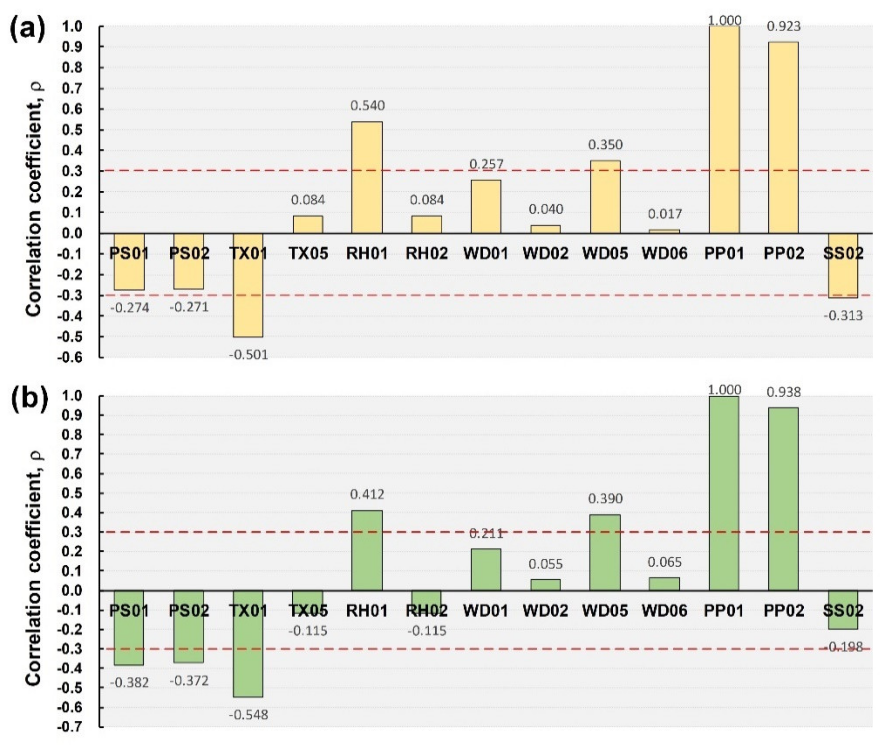
| Attribute (Unit) | Notation | Attribute (Unit) | Notation |
|---|---|---|---|
| Ground air pressure (hPa) | PS01 | Ground vapor pressure (hPa) | RH02 |
| Air pressure at sea level (hPa) | PS02 | Surface wind speed (maximum 10-min mean, | WD01 |
| Ground temperature (°C) | TX01 | 10 m above the surface) (m/s) | |
| Ground dew point temperature (°C) | TX05 | Wind direction of WD01 (deg) | WD02 |
| Ground relative humidity (%) | RH01 | Maximum instantaneous wind speed (m/s) | WD05 |
| Ground global solar radiation (MJ/m2) | SS02 | Wind direction of WD05 (deg) | WD06 |
| Rainfall duration within 1 h (h) | PP02 | Precipitation (mm/h) | PP01 |
| Station | Attribute (Unit) | Min-Max | Mean | St. Dev. |
|---|---|---|---|---|
| Chenggong | Ground temperature, TX01 (°C) | 23.8−33.8 | 27.1 | 1.83 |
| Ground relative humidity, RH01 (%) | 48−100 | 83.7 | 9.82 | |
| Maximum instantaneous wind speed, WD05 (m/s) | 1.6−49.2 | 12.6 | 7.50 | |
| Precipitation, PP01 (mm/h) | 0−66 | 3.41 | 6.96 | |
| Rainfall duration within 1 h, PP02 (h) | 0−1 | 0.47 | 0.46 | |
| Ground global solar radiation, SS02 (MJ/m2) | 0−3.95 | 0.37 | 0.79 | |
| Lanyu | Ground air pressure, PS01 (hPa) | 927.7−975.5 | 962.4 | 7.21 |
| Air pressure at sea level, PS02 (hPa) | 963.1−1012.5 | 998.9 | 7.47 | |
| Ground temperature, TX01 (°C) | 21.9−28.8 | 25.0 | 1.07 | |
| Ground relative humidity, RH01 (%) | 71−100 | 92.1 | 6.12 | |
| Maximum instantaneous wind speed, WD05 (m/s) | 2.3−71.3 | 24.8 | 12 | |
| Precipitation, PP01 (mm/h) | 0−63 | 2.2 | 5.6 | |
| Rainfall duration within 1 h, PP02 (h) | 0−1 | 0.34 | 0.42 |
| Station | Chenggong | Lanyu | ||||
|---|---|---|---|---|---|---|
| Parameter | Learning Rate | Min_Child_Weight | Max_Depth | Learning Rate | Min_Child_Weight | Max_Depth |
| Case 1 | 0.3 | 1 | 3 | 0.2 | 3 | 7 |
| Case 2 | 0.2 | 1 | 7 | 0.2 | 2 | 10 |
| Case 3 | 0.4 | 3 | 9 | 0.3 | 1 | 11 |
| Angle | Chenggong Station | Lanyu Station | ||
|---|---|---|---|---|
| Optimal Model Case | RMSE (mm/h) | Optimal Model Case | RMSE (mm/h) | |
| 0.5° | XGBoost with Case 3 | 2.827 | XGBoost with Case 3 | 2.391 |
| 1.4° | XGBoost with Case 3 | 2.750 | XGBoost with Case 3 | 2.102 |
| 2.4° | XGBoost with Case 3 | 2.832 | XGBoost with Case 3 | 2.087 |
| 3.4° | XGBoost with Case 3 | 2.782 | XGBoost with Case 3 | 2.227 |
| 4.3° | XGBoost with Case 3 | 2.636 | XGBoost with Case 3 | 2.016 |
| 6.0° | XGBoost with Case 3 | 2.520 | XGBoost with Case 3 | 2.289 |
| 9.9° | XGBoost with Case 3 | 2.584 | XGBoost with Case 3 | 2.093 |
| 14.6° | XGBoost with Case 3 | 2.649 | XGBoost with Case 3 | 2.802 |
| 19.5° | XGBoost with Case 3 | 2.761 | XGBoost with Case 3 | 2.532 |
| All | XGBoost with Case 3 | 2.723 | XGBoost with Case 3 | 3.050 |
| Average of all subcases | 2.706 | Average of all subcases | 2.359 | |
© 2020 by the authors. Licensee MDPI, Basel, Switzerland. This article is an open access article distributed under the terms and conditions of the Creative Commons Attribution (CC BY) license (http://creativecommons.org/licenses/by/4.0/).
Share and Cite
Wei, C.-C.; Hsu, C.-C. Extreme Gradient Boosting Model for Rain Retrieval using Radar Reflectivity from Various Elevation Angles. Remote Sens. 2020, 12, 2203. https://doi.org/10.3390/rs12142203
Wei C-C, Hsu C-C. Extreme Gradient Boosting Model for Rain Retrieval using Radar Reflectivity from Various Elevation Angles. Remote Sensing. 2020; 12(14):2203. https://doi.org/10.3390/rs12142203
Chicago/Turabian StyleWei, Chih-Chiang, and Chen-Chia Hsu. 2020. "Extreme Gradient Boosting Model for Rain Retrieval using Radar Reflectivity from Various Elevation Angles" Remote Sensing 12, no. 14: 2203. https://doi.org/10.3390/rs12142203
APA StyleWei, C.-C., & Hsu, C.-C. (2020). Extreme Gradient Boosting Model for Rain Retrieval using Radar Reflectivity from Various Elevation Angles. Remote Sensing, 12(14), 2203. https://doi.org/10.3390/rs12142203