Article

Influence of Soil Properties on Maize and Wheat Nitrogen Status Assessment from Sentinel-2 Data

1
Department of Agricultural and Forestry Scieces (DAFNE), University of Tuscia, Via San Camillo de Lellis, 01100 Viterbo, Italy
2
Institute for Electromagnetic Sensing of the Environment (IREA), Consiglio Nazionale delle Ricerche (CNR), Via Bassini 15, 20133 Milano, Italy
3
IBF Servizi S.p.A. Via Cavicchini, 2 44037 Jolanda di Savoia (Fe), Italy
*
Author to whom correspondence should be addressed.
Remote Sens. 2020, 12(14), 2175; https://doi.org/10.3390/rs12142175
Submission received: 29 May 2020 / Revised: 3 July 2020 / Accepted: 6 July 2020 / Published: 8 July 2020
(This article belongs to the Special Issue Remote Sensing for Sustainable Agriculture and Smart Farming)

Abstract

:
Soil properties variability is a factor that greatly influences cereals crops production and interacts with a proper assessment of crop nutritional status, which is fundamental to support site-specific management able to guarantee a sustainable crop production. Several management strategies of precision agriculture are now available to adjust the nitrogen (N) input to the actual crop needs. Many of the methods have been developed for proximal sensors, but increasing attention is being given to satellite-based N management systems, many of which rely on the assessment of the N status of crops. In this study, the reliability of the crop nutritional status assessment through the estimation of the nitrogen nutrition index (NNI) from Sentinel-2 (S2) satellite images was examined, focusing of the impact of soil properties variability for crop nitrogen deficiency monitoring. Vegetation indices (VIs) and biophysical variables (BVs), such as the green area index (GAI_S2), leaf chlorophyll content (Cab_S2), and canopy chlorophyll content (CCC_S2), derived from S2 imagery, were used to investigate plant N status and NNI retrieval, in the perspective of its use for guiding site-specific N fertilization. Field experiments were conducted on maize and on durum wheat, manipulating 4 groups of plots, according to soil characteristics identified by a soil map and quantified by soil samples analysis, with different N treatments. Field data collection highlighted different responses of the crops to N rate and soil type in terms of NNI, biomass (W), and nitrogen concentration (Na%). For both crops, plots in one soil class (FOR1) evidenced considerably lower values of BVs and stress conditions with respect to others soil classes even for high N rates. Soil samples analyses showed for FOR1 soil class statistically significant differences for pH, compared to the other soil classes, indicating that this property could be a limiting factor for nutrient absorption, hence crop growth, regardless of the amount of N distributed to the crop. The correlation analysis between measured crop related BVs and satellite-based products (VIs and S2_BVs) shows that it is possible to: (i) directly derive NNI from CCC_S2 (R2 = 0.76) and either normalized difference red edge index (NDRE) for maize (R2 = 0.79) or transformed chlorophyll absorption ratio index (TCARI) for durum wheat (R2 = 0.61); (ii) indirectly estimate NNI as the ratio of plant nitrogen uptake (PNUa) and critical plant nitrogen uptake (PNUc) derived using CCC_S2 (R2 = 0.77) and GAI_S2 (R2 = 0.68), respectively. Results of this study confirm that NNI is a good indicator to monitor plants N status, but also highlights the importance of linking this information to soil properties to support N site-specific fertilization in the precision agriculture framework. These findings contribute to rational agro-practices devoted to avoid N fertilization excesses and consequent environmental losses, bringing out the real limiting factors for optimal crop growth.

Graphical Abstract

1. Introduction

Crop nutritional stress is usually assessed considering N deficiency on the base of plant analysis methods with no direct measurements or in consideration of soil properties information. If not considered, soil variability can prevent a correct diagnosis of the nutritional status of crops. The influence of soil properties variations in relation to crop nitrogen status assessment performed with proximal or remote sensing technique is a topic that has not been much studied in literature. As reported by [1], several studies have demonstrated separately the potential advantages of crop spatial variability analysis with soil-based and plant-based methods in order to drive variable N fertilization, but only few studies assessed the interaction between the two, hence the possibility to combine this information in a decision process [1,2].
Cereals cultivation requires sustainability in terms of production and environmental impacts. Nitrogen is one of the most important nutrients for plants. Soil N availability varies spatially and temporally within a field due plant, soil–atmosphere interaction almost guided by the variations of soil properties and land morphology. Crop N demand changes during the season depending on growing conditions related to the presence of limiting factors. This requirement is met by soil N supply capacity and N fertilizations. N mineral fertilizers are globally the most used substances for fertilization, with a world supply of ammonia (NH3) of ~180 million tons [3]. Unfortunately, the large quantities used do not correspond to high levels of nitrogen use efficiency (NUE) [4,5,6,7]. Sustainable agriculture requires optimizing N management during the crop season, in order to achieve profitability and a healthy environment [8,9,10]. N supply from soil and fertilizations and N accumulation in crops are very dynamic processes that should be considered through an integrated approach [11,12] and a spatial relationship analysis [13]. The uncertainty in both plant N demand and soil N supply due to seasonality and growth potential often leads to non-optimal nitrogen management strategies [14].
One of the most widely used crop N status assessment methods relies on the estimation of the nitrogen nutrition index (NNI), defined as the ratio of the actual N concentration in the dry above-ground biomass (Na%) to a critical N concentration (Nc%), which is in relation to the specific above-ground biomass (W) expressed in t ha−1 [14]. NNI can also be derived considering crop N content (kg N ha−1), instead of concentration (%). In this case, NNI is computed using the ratio between actual plant nitrogen uptake (PNUa) and critical plant nitrogen uptake (PNUc), both expressed in kg N ha−1 [15,16]. This is because the amount of N in the plant, expressed as a concentration or quantity, and biomass accumulation, have a relationship based on the theory of N dilution during plant growth [17]. The critical nitrogen dilution curve derived from this theory [18] determines the minimum N concentration (Nc) or N content (PNUc) [16] in the crop, for a specific moment, which allows for a normal growth with no biomass accumulation reduction. Other authors identified N dilution curves as a function of development stages [19,20] or Leaf Area Index (LAI) [16,21,22,23] instead of using W. The use of LAI to obtain NNI estimation is indeed a promising approach, because it can be performed with non-destructive measures of W using in field or remote indirect methods [24,25]. Besides the field estimation of NNI, this indicator can also be calculated by empirical relations with remote sensing (RS) vegetation indices (VIs) or biophysical variables (BV) using proximal or satellite data. RS data can be used to derive both Na% and Nc% (via their relationships with W) or PNUa and PNUc. Many authors suggest that the latter option is preferable, because the relationship between RS data and total quantities of nitrogen present in the canopy is more robust [14,26].
From the literature, two approaches have been used to estimate NNI from satellite data: (1) direct methods (DM) and (2) indirect methods (IM). DM rely on the possibility to estimate NNI by “direct” relationships with Vis. According to [27], we can use a (i) “mechanistic approach” (DM_1) that requires first to estimate Na% and W to calculate NNI or (ii) a “semi–empirical approach” (DM_2) based on the direct definition of a parametric regression between VIs and NNI values that are usually estimated with in situ data. Many authors have successfully used DM of NNI from remote sensing using multispectral [23,28,29,30,31] or hyperspectral data [32,33] for optimizing the timing and the rate of N fertilizer applications. The study of [34] tested a DM_1 approach in an operational workflow for producing NNI maps based on the combined use of high-resolution satellite images and ground-based estimates of crop parameter using smart apps.
IM are based on a different paradigm: RS data are firstly used to retrieve biophysical variables from RS, such as leaf area index (LAI) and canopy chlorophyll content (CCC). Then, from these estimates, a relation with PNUa and W is adopted to derive PNUc according to a crop-specific dilution curve. Once PNUa and PNUc are estimated, NNI is calculated. IM approaches have the advantage to exploit RS data to estimate optically related biophysical variables (BV), hence to be a physically-based solution. BV estimation can be performed using (i) parametric regression methods using Vis [15,35,36,37], (ii) non-parametric machine learning algorithm (e.g., neural network, SVR, PLSR etc.) or by inverting radiative transfer models (RTM) adopting look up table approaches [38] or hybrid methods [39,40,41]. For a detailed review of the different available approaches, see [42]. Recently, the European Space Agency (ESA) Sentinel Application Platform (SNAP) toolbox, reached an operational stage in providing biophysical variables (LAI, fAPAR. fcover, CCC) through a biophysical processor tool based on neural networks [43]. This greatly facilitates the operational adoption of RS products in agricultural management decision support systems.
Under this framework, the objectives of this study were to investigate the robustness and representativeness of nutritional status assessment through the computation of NNI from Sentinel-2 for maize and durum wheat in relation to different nitrogen fertilization levels and soil properties. A field experiment for two consecutive crop seasons was set up to interpret the potential and limits of NNI in identify nitrogen deficiency.
More specifically, Sentinel-2 acquisitions were exploited to analyze spatial and temporal variability of crop status from remote sensing with the following objectives: (i) compare the performances of direct and indirect NNI estimation approaches; (ii) assess the added value of the operational S2-BV product with respect to ad hoc calculated VIs.

2. Materials and Methods

2.1. Study Area and Experimental Design

The study area is located in northern Italy, in the eastern part of the Ferrara province, in the Po valley. This flat area, between the city of Ferrara and the Adriatic Sea, derives from extensive land reclamation works concluded at the beginning of the 20th century. This operation generated new arable lands from zones that were previously permanently flooded marshland. This explains a great deal of heterogeneity in soil properties, affecting yields and crop growth.
A field experiment was carried out at the Bonifiche Ferraresi farm, located in Jolanda di Savoia (FE) (lat. 44°52′26″N, long. 11°56′24″E, elev. −3 m), in the 2018 and 2019 seasons, respectively, on maize and durum wheat. Previously, in 2015, the farm conducted a survey for the determination of soil properties using the automatic resistivity profiler (ARP) geophysical sensor [44] as well as soil sampling. From these data, a soil map of the whole farm was derived by the surveying company (SOING, Livorno, Italy). This information was used to identify areas with contrasting soil properties potentially related to different productivity.
For the 2018 and 2019 experiments, a 16 ha field (Figure 1) was chosen and sown with maize, cv SY HYDRO (Syngenta FAO 700) in 2018 and with durum wheat ODISSEO (Syngenta) in 2019 (Table 1). Four different soil classes, coded as CDS2, JOL3, JOL1, FOR1 were present within the field as detected by a pedological survey conducted in 2015 (Figure 1b). A total of 20 plots were established in the field, in which 5 N fertilizer rates were applied with 4 replicates. Each replicate was located inside one of the identified soil classes (Figure 1b) with the goal of maximizing the intra-field nutritional variability. Plot size, 35 m width by 50 m length, was established based on the width of a variable rate (VR) fertilizer spreader, i.e., Sulky model x36 (Sulky-Burel, Chateaubourg, France), and for being large enough to contain at least 10 pixels of a 10 m resolution S2 image.
The N treatments applied to maize and wheat respectively in the 2018 and 2019 season are reported in Table 2. For both crops, two N treatments (N1 and N2) were below the standard N prescription rate of the farm, in order to create N limiting conditions, whereas two treatments (N3 and N4) were above, to create theoretically non-limiting N conditions. Plots with the N0 treatment were considered as non-fertilized controls, but actually received 10 kg N ha−1 because a uniform basal dressing was applied for both crops at sowing with 125 kg ha−1 of 8-18 fertilizer (i.e., 10 kg N ha−1) as a standard practice at the farm. A uniform basal dressing with 200 kg ha-1 Pheoscor was also applied before sowing for both crops, whereas no K fertilizer was applied because of good soil content.
During the season, top dressing fertilizations with urea using prescription maps were carried out according to phenological key stages (Table 2), with the exception of N0 plots. Application maps (as-applied maps) recorded by the VR spreader system, allowed to check the amount of N provided and the accuracy of the spreading in terms of geolocation. In the 2018 season, the last N application at flowering was carried out with a uniform distribution of N, due to the absence of VR machinery for liquid fertilizer distribution. The field was irrigated by means of a drainage sub-irrigation system (Table 1). Other practices for pest, diseases, and weeds control were adequately carried out according to usual farm management practice for both crops. An effort was made to obtain non-limiting conditions for all factors, except for nitrogen fertilization.

2.2. Field Data Collection

In April 2018, an intensive soil sampling campaign was carried out, stratified in the more contrasting areas identified by the resistivity map of the experimental field, collecting a total of 36 soil samples, from a 0–30 cm depth. The number of samples was chosen in order to have 9 points for each of the soil classes identified from the resistivity map, as a compromise between accuracy and resources available (Figure 1). Soil texture, soil organic matter (SOM), total nitrogen, total organic carbon (TOC), pH, C/N were measured in the laboratory using official standard analytical protocols. Along the season, field measurements were carried out to acquire ground data of crop BVs (Table 2).
An ESU (elementary sample unit) [46] of 20 by 20 m size, was defined at the center of each plot and a Trimble GNSS receiver was used to conduct the measurements at the center of each ESU. A Canon digital camera with a fish-eye lens was used to acquire 16 digital hemispherical photographs (DHP), randomly spread in each ESU, at each date and processed with the Can_Eye V6.494 software [47] to estimate crop green area index (GAI). GAI includes all the green parts of the crop and not just the leaves, as for the leaf area index (LAI). The effective_GAI (GAI_eff), computed by the Can_Eye software, was used and not the true_GAI, considering the fact that the former is more theoretically related to the LAI estimated from satellite images [39,43,48]. Leaf chlorophyll content (Cab – mg cm2 leaf) readings from 60 plants in each ESU were acquired with the Dualex (Force-A, Orsay, France) at each measurement date. GAI_eff and Cab were used to compute the chlorophyll content (CCC) by multiplying these two measured variables. Above ground biomass (W) was measured by harvesting 8 plants for each ESU for maize and 1 m2 of wheat crop, which were then dried in the oven at 80 °C until constant weight. The whole plant samples were then finely ground and used for N content (Na%) determination using the Kjeldhal method. The plant phenological stages were identified and registered using the BBCH scale (Biologische Bundesanstalt, Bundessortenamt and CHemical industry) [45].

2.3. Satellite Data

Sentinel-2 SAFE (Standard Archive Format for Europe) level-2A (Bottom-of-Atmosphere BOA) cloud free images, both from S2-A and S2-B satellites, were downloaded and processed using the sen2r R toolbox [49] to produce L2A products and obtain the VIs listed in Table 3. The ESA SNAP biophysical processor toolbox [43] was used to retrieve the satellite-derived biophysical variables (S2_ BVs) LAI_S2 and CCC_S2. LAI_S2 estimated from remote sensing includes all the green parts of the plant and therefore can be called GAI [48]. This variable is similar to the effective LAI output of CAN_EYE [39,43,48]. CCC_S2 is a quantitative variable (g of chlorophylls a + b per m2 of soil) calculated at canopy level, strongly related to leaf nitrogen content [26,39] and it is directly estimated from the SNAP toolbox (LAIxCab). S2Toolbox level2 biophysical variables algorithms implemented in SNAP [43] allow to estimate GAI and CCC and not Cab. Since Cab estimation is fairly complicated due to the gradient of Cab content in the plant and the complexity of canopy structure that influence the radiometric response, the CCC variable is provided, to avoid ambiguities between the GAI and Cab estimation during the inversion process [43]. The spectral domain where Cab can be estimated with high accuracy is in the visible and near infrared and also GAI is influencing the reflectance in this domain, especially for dense canopies [31]. For this reason, CCC is used as an indicator of N stresses [25,39,50], because it includes information on the leaf nitrogen content and the photosynthetic capability [51].
In the 2018 season, four S2 images acquired after N applications and close to field measurement dates were processed, whereas only one useful S2 image close to the field campaign dates was available in 2019 (Table 2), due to cloud occurrence and lodging problems that affected wheat crop before flowering. A vector layer with plots boundaries was used to extract VIs/BVs values from images considering an internal buffer area. Pixels values were averaged for each plot and compared with ground-measured variables.

2.4. NNI Determination

NNI calculation is based on the concept of the dilution curve [18] derived by the theory of decline of N concentration (Nc%) in plants in relation to their growth [17]. Nc is defined as the minimum N concentration that is necessary to achieve potential non limiting production [61]. The critical N dilution curves of both maize and durum wheat crops were calculated using Equation (1), adopting the crops specific coefficients (a, b) proposed for maize and wheat by [16] (a = 3.4, b = 0.37) and [18] (a = 5.35, b = 0.442), respectively:
Nc   % = aW b ,
where W is above-ground biomass (t ha−1), a represents the plant N concentration when W is 1 t ha−1 and b is a dimensionless coefficient. Nc % is constantly considered 3.4% for W < 1 t ha−1 for maize and 4.4% for W < 1.55 t ha−1 for wheat according to [16,18]. The NNI was calculated using Equation (2) as the ratio between the actual plant N concentration (Na%) and the critical plant N concentration (Nc%):
NNI = Na Nc ,
and was used to define conditions of N deficiency (NNI < 0.9), N surplus (NNI > 1.1), and optimal status (0.9 < NNI < 1.1). NNI can also be determined as the ratio between the actual plant N uptake (PNUa, kg ha−1) and the critical plant N uptake (PNUc, kg ha−1) exploiting the theory of the critical nitrogen absorption curve [15,16]. PNUa and PNUc were calculated by multiplying W by Na% and Nc%, respectively. Excess or deficit of nitrogen uptake can be determined by the relationship between the nitrogen absorbed by the crop (PNUa kg ha−1) and its biomass [15]. Then, a quantitative indicator ΔPNU (kg ha−1) [26] can be determined using Equation (3) and directly used to calculate the N rates (increase or reduction of planned dose) to be considered for site-specific fertilization purpose:
Δ PNU = PNUa PNUc .

2.5. NNI Estimation from Remote Sensing

In this study, two approaches have been tested for NNI calculation from RS data. For method 1, (DM) linear regressions between selected Vis and field measured Na% and NNI were derived, while for method 2, (IM) S2_BVs were first calculated from SNAP biophysical toolbox and then linear regressions to measured PNUa and W was exploited in order to determine NNI. The studies of [15,26] proposed three IM to estimate PNUa and PNUc from remote sensing data for then calculating ΔPNU or NNI, evaluating the third scheme as the best in terms of prediction. This scheme consists of calculating PNUa directly from CCC using experimental relationships and then obtaining PNUc by estimating W from GAI. The NNI values obtained from the two methods were then compared with field measured NNI. In order to further test the information content of NNI as a proxy for nitrogen deficiency diagnosis, an NNI map for all the 2018 maize cultivated fields was produced with S2 data and compared to field level reported yield. The regression model between VIs and BVs calculated from S2 images and crop variables collected during field experiments were analyzed using statistical parameters using R 3.5 version software [62]. The performance of the different regression models was estimated by analyzing the coefficient of determination (R2), mean absolute error (MAE), root mean square error (RMSE) (Table 4).
The results of soil laboratory analyses were assessed using one way analysis of variance (ANOVA) and Tukey HSD post hoc test (p < 0.05) in statistical software R 3.5 version [62] to evaluate differences in soil properties among soil classes.

3. Results

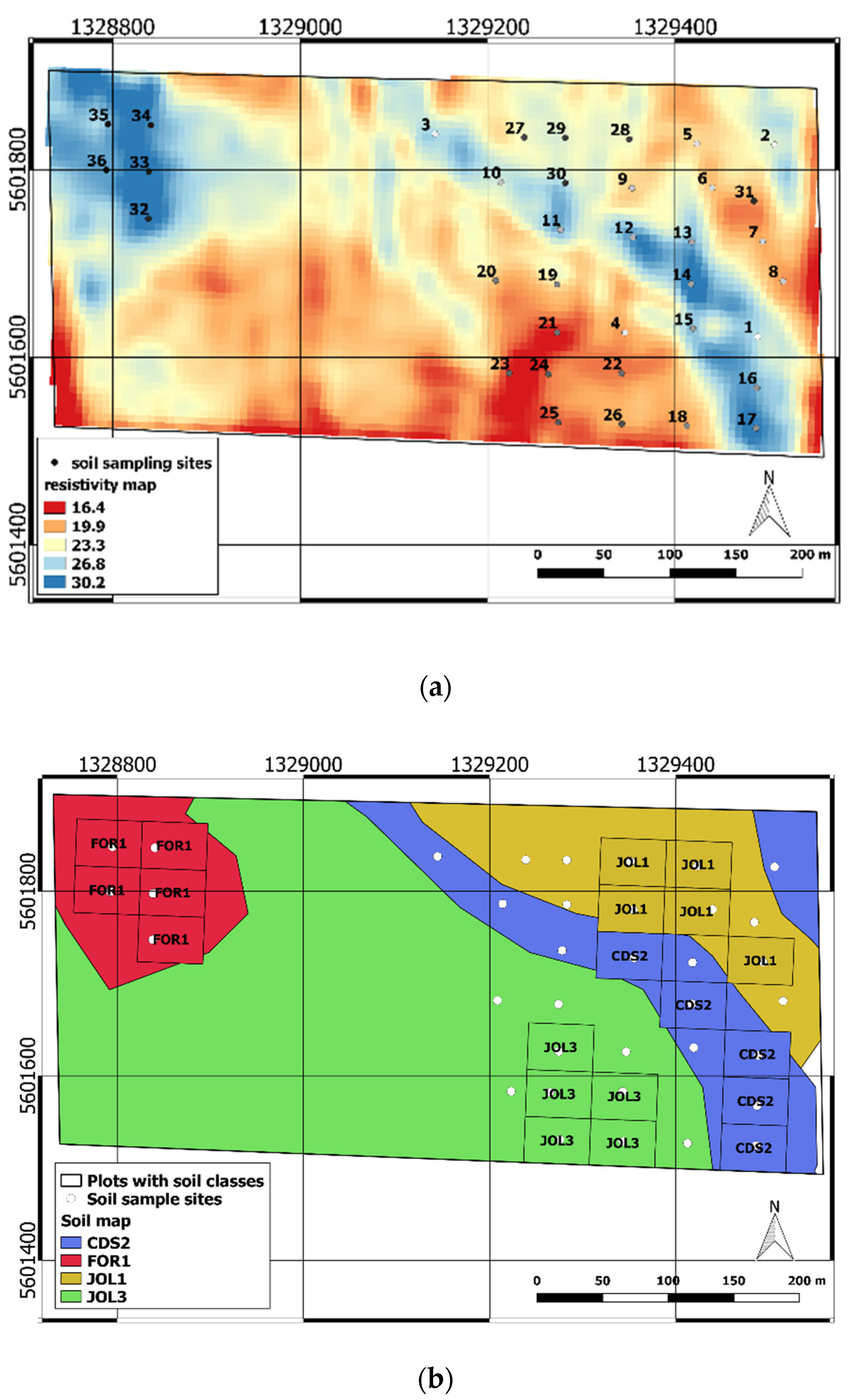
3.1. Soil Variability in the Experimental Field

In general, laboratory analyses revealed that the field had a clay soil (63%) with generally good fertility, as indicated by high total organic carbon (TOC) and soil organic matter (SOM) (6%), moderate total N content (0.34%), and good C/N (10.25%). The comparison among soil classes showed a statistically significant difference in pH and in total N (%) for the FOR1 class with respect to the others (Table 5). The differences in pH, sub-acidic for FOR1 (pH = 5.45) compared to the sub-alkaline of the other classes (pH~7.5), respect to N total content, are considered quite important because of: (i) the general high amount of N total in the soil; (ii) the potential impact of pH on elements availability in the soil for plant nutrition.

3.2. Crop Response to Fertilization and Soil Influence

3.2.1. Plant Growth and Yield

During the 2018 season, maize was harvested at the phenological phase of the milky stage to produce silage of maize mash (grains and maize cob). The harvest was weighed at the farm Weighbridge showing a yield of 14.2 t ha−1. In 2018, the farm harvested 278 ha of silage maize in total, with an overall average yield of 18.22 t ha−1, therefore the experimental field produced less than the farm average (considering FAO 600–700 classes) and less than the variety yield potential (HYDRO FAO 700). The 1st of June 2018 during phase BBCH 15 the whole farm and the experimental field were affected by a hailstorm that caused serious damage to plant foliage with different intensity for each field.
For the maize experiment, crop response to variable N fertilization showed different patterns depending on N rate and soil classes. In general, it is expected that maize biomass would increase with increasing N rates [1,18,31]. In our case, biomass response was strongly influenced by soil properties as shown in Figure 2 and the biomass trends are not always correlated with increasing N rates, indicating that other limiting factors might have affected crop N uptake.
On the first measurement date (09 May, BBCH 12), the effect of N fertilization on maize biomass was still not visible (Figure 2a). On the other dates, whereas for most soil classes, a rate of 90 or 180 kg N ha−1 allowed to reach the maximum biomass, the plots with soil type FOR1 showed a remarkably lower response to N (Figure 2b–d). This effect was probably due to other nutritional limitations, caused by the low pH of this soil class (Table 5). For example, it can be seen from Figure 2, that the JOL1 soil class is characterized by increasing biomass values according to N application on both phases, BBCH 15 (Figure 2b) and BBCH 65 (Figure 2d), whereas the FOR1 soil class remained stable with a lower biomass accumulation. In general, a limited or negative effect on biomass production was obtained for the highest N rates in this experiment. In particular, the range of measured biomass values at flowering (Table 6), which are expected to be related to the final yield, highlights how the biomass values reached in JOL1 almost doubled the biomass level achieved in the FOR1 soil class and how the biomass in the different soil classes are statistically different.
Different N treatments showed a substantial effect on Na% changes across different growth stages, except for the first measurement date (Figure 2). During subsequent growth phases, similar patterns of response of Na% to N rates were observed among the soil classes. Unlike biomass, Na% showed increasing concentration values for increasing N rates in all soil classes. The FOR1 class achieved high concentrations of nitrogen in highly fertilized plots as opposed to what was seen for biomass (Figure 2f–h).
Concerning the durum wheat 2019 experiment, marked effects of different soil classes of the field, on crop response to N rates, were also observed. In Figure 3, the results of only 2 field measurement dates are presented, due to lodging problems caused by wind occurring later in the season. At the BBCH 31 stage, plots in JOL1 registered the highest biomass values (Figure 3b) in all N treatments (reaching 3.24 t ha−1 at the highest N4 rate), while plots in FOR1 yielded the lowest biomass, less than half of the total biomass of JOL1 at the highest N rate (1.1 t ha−1). The interpretation of the Na% trend in wheat is more complex with respect to maize, since no clear response to N rate is visible (Figure 3), especially for the FOR1 soil class, which showed low Na% values for high levels of N fertilization. These results confirm differences of crop response to different soil classes to the N fertilization in both years. In some zones of the field (JOL1, CDS2), the crop manages to reach substantial W and Na% values, even if it is less fertilized, whereas in others, is not able to produce high biomass even if it is highly fertilized (FOR1). An apparent non responsiveness of crop biomass and N content to N fertilization rates in a specific zone of the field, was observed for both seasons and crops, and can be associated to static variables of soil properties, such as in this case, the pH.

3.2.2. Nutritional Status–NNI Values

Figure 4 provides a representation of crop nutritional status for each measured plot in relation to N supply, data are plotted in the W (x-axis) and Na space (y-axis) and compared to the critical N from the dilution curves for maize [16] and durum wheat [18].
The calculated NNI values ranged between 0.42 and 1.12 and 0.43 and 1.15 for maize and wheat respectively, revealing the condition of plot with N deficiency (NNI < 0.9). NNI values under varied N applications did not show a clear gradient as expected and observed in other studies [30].
In Figure 4, the grayscale of the symbols, from light grey to black, is proportional to the N application. It would be expected that brighter grey points (N0 and N1 treatments) are more distant from the critical curve with respect to the darker ones (N3 and N4 treatments). This is visible only for the points corresponding to the low doses (N0-N1-N2), but it is not equally respected for the high doses (N3 and N4), evidencing how other factors might have limited nitrogen uptake and plant growth even in non-limiting N conditions. The NNI values for N0 and N1 generally decreased during all BBCH phases, whereas for N3 and N4 treatment, NNI remained substantially stable (data not shown). NNI values for N3 and N4 treatments in the FOR1 soil class did not reach the value of 1 for both the considered seasons and crops. This finding indicates a sub optimal N condition (Figure 4), whereas CDS2 and JOL2 were very often higher than 0.9. Substantial differences were observed under different soil classes, where classes FOR1 and JOL1 markedly differed in NNI values, especially in N4 treatment. FOR1 had a constant limiting factor that influenced N uptake regardless of N applications.
The boxplot of Figure 5 shows how NNI varied during the growth seasons for maize (2018) and wheat (2019). The general non-optimal nutritional condition of maize and wheat crop in the experiment, especially late in the growth season, is highlighted by many Na% values lower than the critical concentration represented by the dilution curve. Only few plots reached optimal nutritional condition with NNI values greater than 0.9. The effects of soil classes properties on NNI were statistically non-significant (p < 0.05), but FOR1 class, constantly had values unequivocally lower than 0.9 during the season independently of the fertilization rate. Instead, all the plots in classes CDS2 and JOL1 had higher values and no stress for maize (wheat) at BBCH 12 and 30 (25) was detected. The different behavior emerged in the different areas of the field regardless of the nitrogen fertilization class, suggested that the capability of the plants to absorb nutrients and therefore nitrogen depends on different properties of the soil and not only on the quantity of nitrogen that is given with fertilizers. In this case, the sub-acid pH of the FOR1 class limited more the others classes the absorption of nitrogen available in soil and provided by fertilization.

3.3. Remote Sensing Estimation of NNI

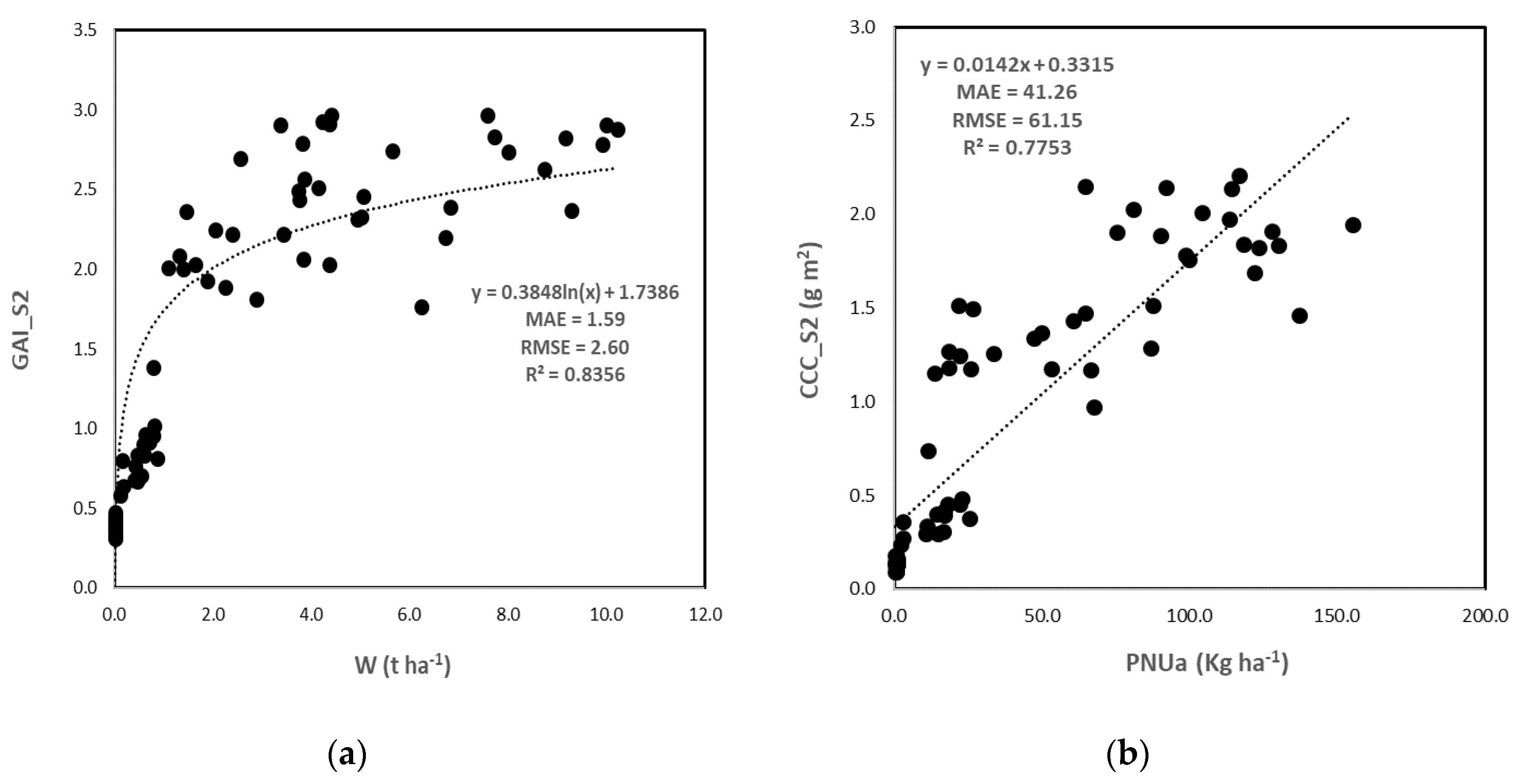
3.3.1. S2 BVs Accuracy

Before considering NNI estimation with indirect methods, S2_BVs retrieval performance was analyzed (Figure 6). From our experimental data, GAI_S2 for maize are well correlated with field estimates (R2 = 0.87 and RMSE = 0.58). Lower performances are obtained for wheat (R2 = 0.41 and RMSE = 0.81), however Sentinel-2 retrievals generally produced higher values than the field measurements, i.e., over-estimation (Figure 6). The obtained accuracy metrics are comparable to those reported by [39], and also in their study, the trend of GAI_S2 values showed some bias (over-estimation).
For what concerns CCC_S2 for maize, the estimations are well correlated with field measurements (R2 = 0.81 and RMSE = 0.67) even though there is an overestimation at the beginning and an underestimation towards the end of the season. Worse performances were obtained for wheat, with R2 = 0.38 and RMSE = 0.72. It is important to note that in 2019 for wheat, a shorter phenological period was monitored due to cloud contamination in EO data that did not allow to analyze images when field data were acquired. These results are in general in agreement with [39,63].

3.3.2. Crop Nutritional Status Estimation

Direct Method

The analyses for maize crop 2018 data (Table 7) show that there were highly significant relationships between NNI and NDRE (R2 = 0.79; RMSE = 0.26; MAE = 0.2) and GNDVI (R2 = 0.77; RMSE = 0.27; MAE = 0.22) (Figure 7). The highest R2 and the smallest RMSE confirm the usefulness of VIs that exploit the red edge spectral region (e.g., NDRE) to provide prediction of leaf N content as mentioned in many studies [36,64,65,66]. We also found a good relationship between Na% and MCARI (R2 = 0.71; RMSE = 2.48; MAE = 2.29), as previously shown for the same crop by [32], but in general, VIs achieved worse results as compared to S2_BV for retrieving BV as W, CCC, and PNUa. For this reason, these results suggest to use VIs to directly derive NNI instead of calculating W and Na% and then indirectly deriving NNI values.
An analysis of the relationships between S2 BV and nutritional status indicators was also performed (Table 7). No index reached the performance of the GAI_S2 for biomass estimation (R2 = 0.68), confirming the correctness in the use of this variable to derive W. Chlorophyll related variables (CCC_S2 and Cab_S2) resulted well correlated with NNI, comparably to VIs analysis, but not so well with Na%. A better relationship was found between NNI and leaf chlorophyll Cab_S2 (R2 = 0.82) where Cab is estimated as the ratio of the two variables output (S2_BVs) from the SNAP Sentinel-2 biophysical processor, i.e., CCC_S2 and GAI_S2. Being Cab_S2 a derived secondary variable, the use of CCC_S2 (R2 = 0.77) in NNI estimation could be preferred to that of the leaf chlorophyll content. In general, good results were found for BV retrieval (W, CCC, PNUa) which suggests the possibility to both use direct or indirect methods to derive NNI.
For wheat crop 2019 data (Table 8), only one S2 image was available during the key phenological phases and close to the field measurements, due to cloud occurrence and the lodging problems that affected the crop before flowering. The partial results for wheat were affected by dependence of the relationship with crop phenology and environmental conditions [39,67] and cannot be a valid exportable predictive model. Despite this, TCARI obtained the best performance in Na% (R2 = 0.61, RMSE = 4.28) and NNI (R2 = 0.61 RMSE = 0.87) retrieval for direct estimation.

Indirect Method

Indirect methods require the capacity to directly estimate different biophysical variables related to crop status. The advantage of using PNUa besides NNI indicator is because it is possible to quantitatively estimate crop N deficit/surplus [15,26] and then use this amount to make N prescription maps. This analysis was performed only on maize data because S2 data were available across the whole 2018 crop season. Figure 8 shows the relationship between GAI_S2 and W for maize, described by a logarithmic function, as expected, with good accuracy R2 = 0.84 and RMSE = 2.60. The variable GAI_S2 can be used to estimate through empirical relationships W. From these estimates, PNUc can be derived using the crop specific critical canopy nitrogen content curve [16,26]. To further calculate ∆PNU, it is crucial to accurately estimate PNUa. The correlation between CCC_S2 and PNUa shows a R2 of 0.77 that is in line with what achieved by [39] and [31], but with an higher RMSE (RMSE = 61.12; MAE = 41.26).
NNI estimates derived from the S2 image of 8th of July with the two methods (direct and indirect) showed similar results if compared with NNI field data. For a single image with direct method and NDRE index, we achieved a R2 of 0.62 (RMSE = 0.21), while when using NNI obtained by the ratio between PNUa and PNUc, we obtained a R2 of 0.63 (RMSE = 0.27).

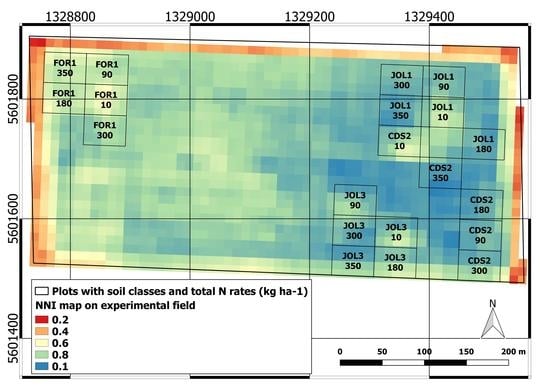
3.3.3. NNI Map and Yield Relation

A NNI map for all the 2018 maize fields of the farm was produced and compared to the reported yield at field level. The S2 image of the 8th of July, corresponding to the end of maize vegetative phase, was used to generate an NNI map using the NDRE relation (Figure 8). The NNI map represents, at the beginning of flowering, when the fertilization period is concluded, a proxy of the potential end-of-season yield if other limiting factors are not occurring (e.g., water stress, pest, disease, or lodging).
The NNI map derived using NDRE showed the variability and the low NNI values of the crop in the experimental field (Figure 9), especially for FOR1 plots (top left of Figure 9). Anova test confirmed that field level NNI values were well correlated with the final yield and maize group (FAO class 600–700) according to nutritional conditions at flowering. The most productive fields had the higher NNI values and vice versa and the NNI map generally predicted well the final yield (Table 9). Correlation analysis between NNI and yield revealed a significant positive correlation (Pearson’s r = 0.6).

4. Discussion

It is recognized that seasonal N status assessment can be performed using the NNI indicator [68], however, not much investigation is present in literature about the interaction between detected crop N deficiency and actual source of crop grow limiting factors. NNI can be used to highlight which zones of a field present crop anomalous conditions: NNI > 1 “luxury consumption” and NNI < 1 “nitrogen deficiency”. Usually this information is used to tactically modulate nitrogen fertilization with VRT machinery, providing the appropriate amount of fertilizer. However, in some cases, plant N deficiency is not related to nitrogen availability, but to other factor that must be identified and taken into account, to support the most appropriate fertilization strategy. The present study highlighted that NNI is an appropriate tool for the diagnosis of the nutritional status of the crops, however, soil properties can have an impact on crop N uptake, showing an effect independent from N rates supply. The capacity of NNI to assess crop nutritional status in relation to soil properties was confirmed for two consecutive crop seasons. In our case, measured NNI showed that the experimental plots located in an area of the field with acidic soil (FOR1) had lower NNI values than all the other plots in the other soils’ types both for maize and wheat. High N rates did not increase Na% and consequently crops biomass in the problematic soil area of the field (FOR1), as expected and as demonstrated by other studies [16,18,29]. In addition to this, the high rate plots in the FOR1 class reached only half of the biomass accumulation (4 t ha−1) as compared to the best performance of JOL1 and CDS2 soil classes (8 t ha−1) and the two classes are statistically different considering this variable. It is well known that most plant nutrients are optimally available to plants within the soil pH range between 6.5 and 7.5 and soil classes of the field experiment belonged to this range except FOR 1. Nutrients absorption depends on elements availability in the root zone and the growth rate potential, even in the N excessive condition, is regulated by the soil N supply [30]. N fertilization can temporarily reduce soil pH in the surface soil layer after the supply, especially at high amounts as demonstrated by [69]. In presence of acidic soils, this effect may be even higher, causing even greater problems in nutrients absorption, with a combination of yield limiting factors. The study of [11] underlined that nitrogen assimilation needs to be considered in the context of inter-regulation of multiple crop physiological processes (i.e., C N assimilation and allocation) and soil N availability.
Besides this consideration, overall, the estimated NNI values during the season have revealed areas with a general sub-optimal crop growth in the experimental field, which resulted in an average yield (14.18 t ha−1) much lower than the average of all the maize fields of the farm (18.22 t ha−1), confirming the goodness of NNI to indicate crop yield potential [14]. NNI calculated from remote sensing during the season resulted in a dynamic diagnostic tool to assess spatial explicit crop N status and limitation in N uptake [14]. NNI calculated from remote sensing during the season resulted in a dynamic diagnostic tool to assess spatial explicit crop N status and limitation in N uptake [14]. Chlorophyll content estimation for crop stress status monitoring has been considered in many studies and for site-specific N management [66,70], but the relationship between chlorophyll content and Na% remains highly empirical [26,71] because it is usually influenced by variety, phenology, and study area, limiting the generalization capability of the method using only chlorophyll content information [39,50]. RS DM are proposed as a rapid and robust way for nutritional status assessment to be used as an alternative to direct field measurements [29,31]. Information on actual nitrogen content or concentration, or direct indication of nitrogen deficiency (NNI) from remote data are of great help in crop monitoring.
From the 2018 maize experiment, we found that the direct estimation of NNI using VIs or S2_BVs derived by Sentinel-2 is feasible as demonstrated by general good correlation metrics comparable to other studies. The best performance was obtained using Cab_S2 secondary variable (R2 = 0.82) slightly better than using CCC_S2 (R2 = 0.77) or NDRE (R2 = 0.79), this performance is similar to what was reported by [65]. Our results indicated also that Na% can be directly derived using MCARI with an agreement of R2 = 0.71, confirming the conclusions of [32]. However, biomass estimation directly from VIs resulted not reliable. So, the direct “mechanistic approach” (DM_2) was not performing as expected. These results confirmed the possibility to directly derive NNI (DM_1) with VIs and/or S2_BVs as a suitable solution for operational crop monitoring to support site-specific nitrogen fertilization. The NNI derived maps showed comparable results in terms of correlation with DM (R2 = 0.62, RMSE = 0.21) and IM (R2 = 0.63, RMSE = 0.27) approaches.
Indirect method (IM) derive NNI from the separate estimations of W and PNUa. The advantage of using such approach is that estimated PNUa can be used to compute ∆PNU, this is a promising quantitative approach to define nitrogen absorption deficit of a crop [14,15,26]. PNUA (kg ha−1) is a quantitative variable preferred over a variable expressed in percentage as Na because it avoids an intermediate step to convert N contents from a mass basis to an area basis to a mass basis [72] as reported by [14]. Experimental results demonstrated that the biophysical variable CCC estimated from S2 is well related with PNUa (R2 = 0.78), confirming the results of previous studies [31,39]. S2 estimated GAI can be used to estimate W (R2 = 0.84), since this variable is necessary to calculate PNUc according to crop specific dilution curves. The quantitative deficit or surplus values given by the indicator ∆PNU is thus suitable for adjusting N supply in site-specific fertilization management.

5. Conclusions

The present study highlighted that soil types have an effect on the diagnosis of the nutritional status of the crops in response to N rates supply. Sentinel-2 data can be exploited to estimate nutritional deficit or surplus computing NNI with direct and indirect methods. In addition to this indicator using indirect methods, it is possible to quantitatively defined the required N amount to supply with VRT machinery by calculating ∆PNU. However, this information is not sufficient and it is necessary to take in account the potential causes of crop nutritional status such as soil properties variability. In the experiment presented here, a limiting factor for optimal crop growth was identified in the soil properties (pH) that reduce the capacity of the crop to uptake N, also in conditions of high N availability in the soil and supplied by fertilization. This influences the interpretation of N status, because even though a nitrogen deficit is detected (i.e., NNI < 0.9) a supplementary provision of fertilizer (∆PNU) would not be efficient. The experiment confirmed that different soils types within a cultivated field can have an effect on growth independently of N rates provided and consequently impact on dry matter production and final yield. Indeed, in the location of a field where yield potential is low, added N fertilizer profitability can be reduced as demonstrated, for example by [73]. The results confirm that, since crop N absorption is a very dynamic and complex process, site-specific management in a precision farming paradigm requires a combination of spatial explicit information: static maps describing variability of soil properties and seasonal information related to actual crop nutritional status achievable from RS data. The information from soil characterization is potentially complementary to crop N status monitoring, and could improve NUE and site-specific N fertilization strategies of cereals cropping systems. Further experiments and tests are needed in different study areas and exploiting data acquired on different seasons to deeply investigate the effect of different soil properties and N supply on crop N deficiency diagnosis and to explore the possibility of using soil and crop derived information in combination.

Author Contributions

“Conceptualization, A.C., R.C. and M.B.; methodology, A.C., R.C. and M.B.; software, A.C and F.N.; validation, A.C., R.C. and M.B.; formal analysis, A.C., R.C., M.B. and F.N.; investigation, A.C., R.C. and F.N.; resources, R.C., M.B. and D.C.; data curation, A.C., R.C., M.B. and F.N.; writing—original draft preparation, A.C.; writing—review and editing, A.C., R.C., M.B., and F.N.; visualization, A.C. and F.N.; supervision, R.C.; project administration, A.C. and R.C; funding acquisition, R.C. All authors have read and agreed to the published version of the manuscript.”

Funding

This research was funded by the company IBF Servizi Spa in the framework of a scientific collaboration agreement with the University of Tuscia. A.C. PhD is funded by University of Tuscia and CNR-IREA.

Acknowledgments

The authors would like to thank the staff of Bonifiche Ferraresi SpA and IBF Servizi SpA for their technical assistance and for their support during the field experiment. The authors would also like to thank Pietro Marino, Paolo Villa, Francesco Mastromauro and Giampiero Ubertini for help with samples analysis and field campaigns. The authors gratefully acknowledge MIUR (Minister for education, University and Research) for financial support (Law 232/216, Department of Excellence) to DAFNE.

Conflicts of Interest

The authors declare no conflict of interest. The funders had no role in the design of the study; in the collection, analyses, or interpretation of data; in the writing of the manuscript, or in the decision to publish the results.

References

  1. Cordero, E.; Longchamps, L.; Khosla, R.; Sacco, D. Spatial management strategies for nitrogen in maize production based on soil and crop data. Sci. Total Environ. 2019, 697, 133854. [Google Scholar] [CrossRef] [PubMed]
  2. Longchamps, L.; Khosla, R. Improving N use efficiency by integrating soil and crop properties for variable rate N management. In Precision Agriculture 2015—Papers Presented at the 10th European Conference on Precision Agriculture, ECPA 2015; Wageningen Academic Publishers: Wageningen, The Netherlands, 2015; pp. 249–255. [Google Scholar]
  3. FAO. World Fertilizer Trends and Outlook to 2018; Food and Agriculture Organization of the United Nations: Rome, Italy, 2015; ISBN 9789251086926. [Google Scholar]
  4. Dordas, C.A. Nitrogen nutrition index and its relationship to N use efficiency in linseed. Eur. J. Agron. 2011, 34, 124–132. [Google Scholar] [CrossRef]
  5. Cui, Z.; Chen, X.; Zhang, F. Current Nitrogen management status and measures to improve the intensive wheat-maize system in China. Ambio 2010, 39, 376–384. [Google Scholar] [CrossRef] [Green Version]
  6. Lassaletta, L.; Billen, G.; Grizzetti, B.; Anglade, J.; Garnier, J. 50 year trends in nitrogen use efficiency of world cropping systems: The relationship between yield and nitrogen input to cropland. Environ. Res. Lett. 2014, 9, 105011. [Google Scholar] [CrossRef]
  7. Caviglia, O.P.; Melchiori, R.J.M.; Sadras, V.O. Nitrogen utilization efficiency in maize as affected by hybrid and N rate in late-sown crops. Field Crops Res. 2014, 168, 27–37. [Google Scholar] [CrossRef]
  8. Stamatiadis, S.; Schepers, J.S.; Evangelou, E.; Tsadilas, C.; Glampedakis, A.; Glampedakis, M.; Dercas, N.; Spyropoulos, N.; Dalezios, N.R.; Eskridge, K. Variable-rate nitrogen fertilization of winter wheat under high spatial resolution. Precis. Agric. 2018, 19, 570–587. [Google Scholar] [CrossRef]
  9. Diacono, M.; Rubino, P.; Montemurro, F. Precision nitrogen management of wheat. A review. Agron. Sustain. Dev. 2013, 33, 219–241. [Google Scholar] [CrossRef]
  10. Bongiovanni, R.; Lowenberg-Deboer, J. Precision agriculture and sustainability. Precis. Agric. 2004, 5, 359–387. [Google Scholar] [CrossRef]
  11. Gastal, F.; Lemaire, G. N uptake and distribution in crops: An agronomical and ecophysiological perspective. J. Exp. Bot. 2002, 53, 789–799. [Google Scholar] [CrossRef] [Green Version]
  12. Körschens, M.; Albert, E.; Armbruster, M.; Barkusky, D.; Baumecker, M.; Behle-Schalk, L.; Bischoff, R.; Čergan, Z.; Ellmer, F.; Herbst, F.; et al. Effect of mineral and organic fertilization on crop yield, nitrogen uptake, carbon and nitrogen balances, as well as soil organic carbon content and dynamics: Results from 20 European long-term field experiments of the twenty-first century. Arch. Agron. Soil Sci. 2013, 59, 1017–1040. [Google Scholar] [CrossRef]
  13. Casa, R.; Castrignanò, A. Analysis of spatial relationships between soil and crop variables in a durum wheat field using a multivariate geostatistical approach. Eur. J. Agron. 2008, 28, 331–342. [Google Scholar] [CrossRef] [Green Version]
  14. Lemaire, G.; Jeuffroy, M.H.; Gastal, F. Diagnosis tool for plant and crop N status in vegetative stage. Theory and practices for crop N management. Eur. J. Agron. 2008, 28, 614–624. [Google Scholar] [CrossRef]
  15. Guerif, M.; Houlès, V.; Baret, F. Remote sensing and detection of nitrogen status in crops. Application to precise nitrogen fertilization. In Proceedings of the 4th International Symposium on Intelligent Information Technology in Agriculture, Beijing, China, 26–29 October 2007; p. 19. [Google Scholar]
  16. Plénet, D.; Lemaire, G. Relationships between dynamics of nitrogen uptake and dry matter accumulation in maize crops. Determination of critical N concentration. Plant Soil 2000, 216, 65–82. [Google Scholar] [CrossRef]
  17. Greenwood, D.J.; Lemaire, G.; Gosse, G.; Cruz, P.; Draycott, A.; Neeteson, J.J. Decline in Percentage N of C3 and C4 Crops with Increasing Plant Mass. Ann. Bot. 1990, 66, 425–436. [Google Scholar] [CrossRef] [Green Version]
  18. Justes, E.; Mary, B.; Meynard, J.-M.; Machet, J.-M.; Thelier-Huche, L. Determination of critical nitrogen dilution curve for winter wheat crops. Ann. Bot. 1994, 74, 397–404. [Google Scholar] [CrossRef]
  19. Williams, J.R.; Jones, C.A.; Kiniry, J.R.; Spanel, D.A. The EPIC Crop Growth Model. Trans. ASAE 1989, 32, 497–511. [Google Scholar] [CrossRef]
  20. Hansen, S.; Jensen, H.E.; Nielsen, N.E.; Svendsen, H. Simulation of nitrogen dynamics and biomass production in winter wheat using the Danish simulation model DAISY. Fertil. Res. 1991, 27, 245–259. [Google Scholar] [CrossRef]
  21. Grindlay, D.J.C.; Sylvester-Bradley, R.; Scott, R.K. Nitrogen uptake of young vegetative plants in relation to green area. J. Sci. Food Agric. 1993, 63, 116. [Google Scholar]
  22. Zhao, B.; Yao, X.; Tian, Y.C.; Liu, X.J.; Ata-Ul-Karim, S.T.; Ni, J.; Cao, W.X.; Zhu, Y. New critical nitrogen curve based on leaf area index for winter wheat. Agron. J. 2014, 106, 379–389. [Google Scholar] [CrossRef]
  23. Ata-Ul-Karim, S.T.; Zhu, Y.; Yao, X.; Cao, W. Determination of critical nitrogen dilution curve based on leaf area index in rice. Field Crops Res. 2014, 167, 76–85. [Google Scholar] [CrossRef]
  24. Confalonieri, R.; Debellini, C.; Pirondini, M.; Possenti, P.; Bergamini, L.; Barlassina, G.; Bartoli, A.; Agostoni, E.G.; Appiani, M.; Babazadeh, L.; et al. A new approach for determining rice critical nitrogen concentration. J. Agric. Sci. 2011, 149, 633–638. [Google Scholar] [CrossRef]
  25. Weiss, M.; Baret, F.; Myneni, R.B.; Pragnère, A.; Knyazikhin, Y. Investigation of a model inversion technique to estimate canopy biophysical variables from spectral and directional reflectance data. Agronomie 2000, 20, 3–22. [Google Scholar] [CrossRef]
  26. Houlès, V.; Guérif, M.; Mary, B. Elaboration of a nitrogen nutrition indicator for winter wheat based on leaf area index and chlorophyll content for making nitrogen recommendations. Eur. J. Agron. 2007, 27, 1–11. [Google Scholar] [CrossRef]
  27. Chen, P. A comparison of two approaches for estimating the wheat nitrogen nutrition index using remote sensing. Remote Sens. 2015, 7, 4527–4548. [Google Scholar] [CrossRef] [Green Version]
  28. Huang, S.; Miao, Y.; Zhao, G.; Yuan, F.; Ma, X.; Tan, C.; Yu, W.; Gnyp, M.L.; Lenz-Wiedemann, V.I.S.; Rascher, U.; et al. Satellite remote sensing-based in-season diagnosis of rice nitrogen status in Northeast China. Remote Sens. 2015, 7, 10646–10667. [Google Scholar] [CrossRef] [Green Version]
  29. Zhao, B.; Duan, A.; Ata-Ul-Karim, S.T.; Liu, Z.; Chen, Z.; Gong, Z.; Zhang, J.; Xiao, J.; Liu, Z.; Qin, A.; et al. Exploring new spectral bands and vegetation indices for estimating nitrogen nutrition index of summer maize. Eur. J. Agron. 2018, 93, 113–125. [Google Scholar] [CrossRef]
  30. Zhao, B.; Ata-Ul-Karim, S.T.; Duan, A.; Liu, Z.; Wang, X.; Xiao, J.; Liu, Z.; Qin, A.; Ning, D.; Zhang, W.; et al. Determination of critical nitrogen concentration and dilution curve based on leaf area index for summer maize. Field Crops Res. 2018, 228, 195–203. [Google Scholar] [CrossRef]
  31. Xia, T.; Miao, Y.; Wu, D.; Shao, H.; Khosla, R.; Mi, G.; Xia, T.; Miao, Y.; Wu, D.; Shao, H.; et al. Active Optical Sensing of Spring Maize for In-Season Diagnosis of Nitrogen Status Based on Nitrogen Nutrition Index. Remote Sens. 2016, 8, 605. [Google Scholar] [CrossRef] [Green Version]
  32. Cilia, C.; Panigada, C.; Rossini, M.; Meroni, M.; Busetto, L.; Amaducci, S.; Boschetti, M.; Picchi, V.; Colombo, R. Nitrogen status assessment for variable rate fertilization in maize through hyperspectral imagery. Remote Sens. 2014, 6, 6549–6565. [Google Scholar] [CrossRef] [Green Version]
  33. Wang, R.; Song, X.; Li, Z.; Yang, G.; Guo, W.; Tan, C.; Chen, L. Estimation of winter wheat nitrogen nutrition index using hyperspectral remote sensing. Trans. Chin. Soc. Agric. Eng. 2014, 30, 191–198. [Google Scholar] [CrossRef]
  34. Nutini, F.; Confalonieri, R.; Crema, A.; Movedi, E.; Paleari, L.; Stavrakoudis, D.; Boschetti, M. An operational workflow to assess rice nutritional status based on satellite imagery and smartphone apps. Comput. Electron. Agric. 2018, 154, 80–92. [Google Scholar] [CrossRef]
  35. Blondlot, A.; Gate, P.; Poilvé, H. Providing operational nitrogen recommendations to farmers using satellite imagery. Precis. Agric. 2005, 5, 345–352. [Google Scholar]
  36. Feng, W.; Guo, B.B.; Zhang, H.Y.; He, L.; Zhang, Y.S.; Wang, Y.H.; Zhu, Y.J.; Guo, T.C. Remote estimation of above ground nitrogen uptake during vegetative growth in winter wheat using hyperspectral red-edge ratio data. Field Crops Res. 2015, 180, 197–206. [Google Scholar] [CrossRef]
  37. Clevers, J.G.P.W.; Kooistra, L.; van den Brande, M.M.M. Using Sentinel-2 data for retrieving LAI and leaf and canopy chlorophyll content of a potato crop. Remote Sens. 2017, 9, 405. [Google Scholar] [CrossRef] [Green Version]
  38. Berger, K.; Atzberger, C.; Danner, M.; D’Urso, G.; Mauser, W.; Vuolo, F.; Hank, T. Evaluation of the PROSAIL model capabilities for future hyperspectral model environments: A review study. Remote Sens. 2018, 10, 85. [Google Scholar] [CrossRef] [Green Version]
  39. Delloye, C.; Weiss, M.; Defourny, P. Retrieval of the canopy chlorophyll content from Sentinel-2 spectral bands to estimate nitrogen uptake in intensive winter wheat cropping systems. Remote Sens. Environ. 2018, 216, 245–261. [Google Scholar] [CrossRef]
  40. Castaldi, F.; Casa, R.; Pelosi, F.; Yang, H. Influence of acquisition time and resolution on wheat yield estimation at the field scale from canopy biophysical variables retrieved from SPOT satellite data. Int. J. Remote Sens. 2015, 36, 2438–2459. [Google Scholar] [CrossRef]
  41. Upreti, D.; Huang, W.; Kong, W.; Pascucci, S.; Pignatti, S.; Zhou, X.; Ye, H.; Casa, R. A comparison of hybrid machine learning algorithms for the retrieval of wheat biophysical variables from sentinel-2. Remote Sens. 2019, 11, 481. [Google Scholar] [CrossRef] [Green Version]
  42. Verrelst, J.; Malenovský, Z.; Van der Tol, C.; Camps-Valls, G.; Gastellu-Etchegorry, J.P.; Lewis, P.; North, P.; Moreno, J. Quantifying Vegetation Biophysical Variables from Imaging Spectroscopy Data: A Review on Retrieval Methods. Surv. Geophys. 2019, 40, 589–629. [Google Scholar] [CrossRef] [Green Version]
  43. Weiss, M.; Baret, F. S2ToolBox Level 2 Products: LAI, FAPAR, FCOVER- VERSION 1.1; INRA: Avignone, France, 2016. [Google Scholar]
  44. Priori, S.; Martini, E.; Andrenelli, M.C.; Magini, S.; Agnelli, A.E.; Bucelli, P.; Biagi, M.; Pellegrini, S.; Costantini, E.A.C. Improving Wine Quality through Harvest Zoning and Combined Use of Remote and Soil Proximal Sensing. Soil Sci. Soc. Am. J. 2013, 77, 1338. [Google Scholar] [CrossRef]
  45. Lancashire, P.D.; Bleiholder, H.; Boom, T.V.D.; Langelüddeke, P.; Stauss, R.; Weber, E.; Witzenberger, A. A uniform decimal code for growth stages of crops and weeds. Ann. Appl. Biol. 1991, 119, 561–601. [Google Scholar] [CrossRef]
  46. Camacho, F.; Lacaze, R.; Latorre, C.; Baret, F.; De la Cruz, F.; Demarez, V.; Di Bella, C.; Fang, H.; García-Haro, J.; Gonzalez, M.P.; et al. A Network of Sites for Ground Biophysical Measurements in support of Copernicus Global Land Product Validation. Fourth Recent Adv. Quant. Remote Sens. 2014, 1, 1–6. [Google Scholar]
  47. Demarez, V.; Duthoit, S.; Baret, F.; Weiss, M.; Dedieu, G. Estimation of leaf area and clumping indexes of crops with hemispherical photographs. Agric. For. Meteorol. 2008, 148, 644–655. [Google Scholar] [CrossRef] [Green Version]
  48. Duveiller, G.; Weiss, M.; Baret, F.; Defourny, P. Retrieving wheat Green Area Index during the growing season from optical time series measurements based on neural network radiative transfer inversion. Remote Sens. Environ. 2011, 115, 887–896. [Google Scholar] [CrossRef]
  49. Ranghetti, L.; Boschetti, M.; Nutini, F.; Busetto, L. “sen2r”: An R toolbox for automatically downloading and preprocessing Sentinel-2 satellite data. Comput. Geosci. 2020, 139, 104473. [Google Scholar] [CrossRef]
  50. Baret, F.; Houlès, V.; Guérif, M. Quantification of plant stress using remote sensing observations and crop models: The case of nitrogen management. J. Exp. Bot. 2007, 58, 869–880. [Google Scholar] [CrossRef] [PubMed] [Green Version]
  51. Green, D.S.; Erickson, J.E.; Kruger, E.L. Foliar morphology and canopy nitrogen as predictors of light-use efficiency in terrestrial vegetation. Agric. For. Meteorol. 2003, 15, 163–171. [Google Scholar] [CrossRef]
  52. Rouse, J.W.; Haas, R.H.; Schell, J.A.; Deering, D.W. Monitoring vegetation systems in the Great Plains with ERTS. In Proceedings of the Third ERTS Symposium, NASA SP-351, Washington, DC, USA, 10–14 December 1973; Volume 1, pp. 309–317. [Google Scholar]
  53. Barnes, E.M.; Clarke, T.R.; Richards, S.E.; Colaizzi, P.D.; Haberland, J.; Kostrzewski, M.; Waller, P.; Choi, C.; Riley, E.; Thompson, T.; et al. Coincident detection of crop water stress, nitrogen status and canopy density using ground-based multispectral data. In Proceedings of the 5th International Conference on Precision Agriculture, Bloomington, MN, USA, 16–19 July 2000; pp. 1–15. [Google Scholar]
  54. Qi, J.; Chehbouni, A.; Huete, A.R.; Kerr, Y.H.; Sorooshian, S. A modified soil adjusted vegetation index. Remote Sens. Environ. 1994, 48, 119–126. [Google Scholar] [CrossRef]
  55. Gitelson, A.A.; Kaufman, Y.J.; Merzlyak, M.N. Use of a green channel in remote sensing of global vegetation from EOS- MODIS. Remote Sens. Environ. 1996, 58, 289–298. [Google Scholar] [CrossRef]
  56. Daughtry, C.S.T.; Walthall, C.L.; Kim, M.S.; De Colstoun, E.B.; McMurtrey, J.E. Estimating corn leaf chlorophyll concentration from leaf and canopy reflectance. Remote Sens. Environ. 2000, 74, 229–239. [Google Scholar] [CrossRef]
  57. Haboudane, D.; Miller, J.R.; Pattey, E.; Zarco-Tejada, P.J.; Strachan, I.B. Hyperspectral vegetation indices and novel algorithms for predicting green LAI of crop canopies: Modeling and validation in the context of precision agriculture. Remote Sens. Environ. 2004, 90, 337–352. [Google Scholar] [CrossRef]
  58. Rondeaux, G.; Steven, M.; Baret, F. Optimization of soil-adjusted vegetation indices. Remote Sens. Environ. 1996, 55, 95–107. [Google Scholar] [CrossRef]
  59. Haboudane, D.; Miller, J.R.; Tremblay, N.; Zarco-Tejada, P.J.; Dextraze, L. Integrated narrow-band vegetation indices for prediction of crop chlorophyll content for application to precision agriculture. Remote Sens. Environ. 2002, 81, 416–426. [Google Scholar] [CrossRef]
  60. Hunt, E.R.; Doraiswamy, P.C.; McMurtrey, J.E.; Daughtry, C.S.T.; Perry, E.M.; Akhmedov, B. A visible band index for remote sensing leaf chlorophyll content at the Canopy scale. Int. J. Appl. Earth Obs. Geoinf. 2012, 21, 103–112. [Google Scholar] [CrossRef] [Green Version]
  61. Ulrich, A. Physiological Bases for Assessing the Nutritional Requirements of Plants. Ann. Rev. Plant Physiol. 1952, 3, 207–228. [Google Scholar] [CrossRef]
  62. R Core Team. R: A Language and Environment for Statistical Computing; R Foundation for Statistical Computing: Vienna, Austria, 2018. [Google Scholar]
  63. Sehgal, V.K.; Chakraborty, D.; Sahoo, R.N. Inversion of radiative transfer model for retrieval of wheat biophysical parameters from broadband reflectance measurements. Inf. Process. Agric. 2016, 3, 107–118. [Google Scholar] [CrossRef] [Green Version]
  64. Cammarano, D.; Fitzgerald, G.; Basso, B.; O’Leary, G.; Chen, D.; Grace, P.; Fiorentino, C. Use of the Canopy Chlorophyl Content Index (CCCI) for remote estimation of wheat nitrogen content in rainfed environments. Agron. J. 2011, 103, 1597–1603. [Google Scholar] [CrossRef]
  65. Li, F.; Miao, Y.; Feng, G.; Yuan, F.; Yue, S.; Gao, X.; Liu, Y.; Liu, B.; Ustin, S.L.; Chen, X. Improving estimation of summer maize nitrogen status with red edge-based spectral vegetation indices. Field Crops Res. 2014, 157, 111–123. [Google Scholar] [CrossRef]
  66. Miao, Y.; Mulla, D.J.; Randall, G.W.; Vetsch, J.A.; Vintila, R. Combining chlorophyll meter readings and high spatial resolution remote sensing images for in-season site-specific nitrogen management of corn. Precis. Agric. 2009, 10, 45–62. [Google Scholar] [CrossRef]
  67. Hamblin, J.; Stefanova, K.; Angessa, T.T. Variation in chlorophyll content per unit leaf area in spring wheat and implications for selection in segregating material. PLoS ONE 2014, 9, e92529. [Google Scholar] [CrossRef] [Green Version]
  68. Lemaire, G.; Meynard, J.M. Use of the Nitrogen Nutrition Index for the Analysis of Agronomical Data. In Diagnosis of the Nitrogen Status in Crops; Lemaire, G., Ed.; Springer: Berlin/Heidelberg, Germany, 1997; pp. 45–55. ISBN 978-3-642-60684-7. [Google Scholar]
  69. Schroder, J.L.; Zhang, H.; Girma, K.; Raun, W.R.; Penn, C.J.; Payton, M.E. Soil acidification from long-term use of nitrogen fertilizers on winter wheat. Soil Sci. Soc. Am. J. 2011, 75, 957–964. [Google Scholar] [CrossRef]
  70. Han, S.; Hendrickson, L.L.; Ni, B. Comparison of satellite and aerial imagery for detecting leaf chlorophyll content in corn. Trans. Am. Soc. Agric. Eng. 2002, 45, 1229–1236. [Google Scholar] [CrossRef]
  71. Lemaire, G.; van Oosterom, E.; Sheehy, J.; Jeuffroy, M.H.; Massignam, A.; Rossato, L. Is crop N demand more closely related to dry matter accumulation or leaf area expansion during vegetative growth? Field Crops Res. 2007, 100, 91–106. [Google Scholar] [CrossRef]
  72. Roderick, M.L.; Berry, S.L.; Noble, I.R.; Farquhar, G.D. A theoretical approach to linking the composition and morphology with the function of leaves. Funct. Ecol. 1999, 13, 683–695. [Google Scholar] [CrossRef]
  73. Ma, B.-L.; Biswas, D.K. Precision Nitrogen Management for Sustainable Corn Production. In Sustainable Agriculture Reviews; Springer: Cham, Switzerland, 2015; pp. 33–62. [Google Scholar]
Figure 1. Experimental field: (a) soil resistivity map (Ω m2) 0–50 cm depth profile and localization of the 36 soil samples collected in the field; (b) localization of the 20 experimental plots, based on the soil map and on contrasting areas of resistivity map (5 plots for each soil class).
Remotesensing 12 02175 g001
Figure 2. Response of maize above ground biomass and Na% to N fertilizer rates, measured during the 2018 field campaigns in the different soil classes (see Table 5): (a) 09-May BBCH 12; (b) 29-May BBCH 15; (c) 18-Jun BBCH 30; (d) 03-Jul BBCH 65. Plant nitrogen concentration (e) 09-May BBCH 12; (f) 29-May BBCH 15; (g) 18-Jun BBCH 30; (h) 03-Jul BBCH 65. * Na% missing values for the FOR1 class due to samples contamination.
Remotesensing 12 02175 g002
Figure 3. Response of wheat above ground biomass (W) and Na% to N fertilizer rates, measured during the 2019 field campaigns in the different soil classes (see Table 5): (a) W at 19 Mar BBCH 25; (b) W at 19 Apr BBCH 31; (c) Na% at 19 Mar BBCH 25; (d) Na% at 19 Apr BBCH 31.
Remotesensing 12 02175 g003
Figure 4. Relationships between biomass and N content for different soil classes at different N rates compared to the crop specific critical N dilution curve for maize and wheat.
Remotesensing 12 02175 g004
Figure 5. Boxplot of Nitrogen Nutrition Index (NNI) values during different phenological phases according to soil classes identified in Table 5. All 5 N treatments are included in each boxplot. Dot lines at NNI of 0.9 and 1.1 represent good nutritional conditions of the crop.
Remotesensing 12 02175 g005
Figure 6. Scatterplot and statistics computed for Green Area Index (GAI) and Canopy Chlorophyll Content (CCC) retrieved from Sentinel-2 images. Relationships in maize crop from the 2nd leaf stage to silking stage (4 S2 images) between: (a) GAI estimated from S2 (GAI_S2) and measured GAI (GAI_DHP_effective); (b) CCC from S2 (CCC_S2) and measured CCC (Cab Dualex × GAI_DHP_eff). Relationships in wheat crop for tillering between: (c) GAI from S2 (GAI_S2) and measured GAI (GAI_DHP_effective); (d) CCC estimated from S2 (CCC_S2) and measured CCC (Cab Dualex × GAI_DHP_eff).
Remotesensing 12 02175 g006
Figure 7. Scatterplots and statistics for S2_BVs and VIs derived from Sentinel-2 data (4 S2 images) and field data from 2nd leaf stage to silking stage in maize crop 2018. Relationships between: (a) normalized difference red edge index (NDRE) and nitrogen nutrition index (NNI) from ground data; (b) modified chlorophyll absorption in reflectance index (MCARI) and plant nitrogen content (Na%) from ground data; (c) chlorophyll content (Cab_S2 from S2 (GAI_S2/CCC_S2) and nitrogen nutrition index (NNI) from ground data; (d) chlorophyll content (Cab_S2 from S2 (GAI_S2/CCC_S2) and plant nitrogen content (Na%).
Remotesensing 12 02175 g007
Figure 8. Relationships between biophysical variables retrieved from Sentinel-2 (4 S2 images) and ground measured in maize crop 2018; (a) above ground biomass (W) and green area index from S2 (GAI_S2); (b) nitrogen uptake (PNUa) and canopy chlorophyll content from S2 (CCC_S2).
Remotesensing 12 02175 g008
Figure 9. NNI map derived on the experimental field with the direct method from the NDRE of the S2 image of 08-July. Rectangles show the locations of the plots, the corresponding soil classes (see Figure 1), and total N rates provided during the season (kg N ha−1).
Remotesensing 12 02175 g009
Table 1. Agronomic details of field experiments for maize in 2018 and wheat in 2019.
VarietyDensity Plowing DatePlanting DateHarvest DateIrrigation
MaizeSY8.8 seeds m22-Apr 201817-Apr 201825-Aug 2018Sub-irrigation
WheatODISSEO200 kg ha−120-Oct 201812-Nov 201815-Jun 2019No irrigation
Table 2. Experimental design details.
YearCropN Treat. CodeN Rate
(kg N ha−1)
BBCH aN Application DateBBCH bField Campaign DateBBCH cS2 Acquisition Date
2018MaizeN010
N19000 d17-Apr1209-May1319-May
N21801321-May1529-May1603-Jun
N33001601-Jun3018-Jun5023-Jun
N43506026-Jun6503-Jul6508-Jul
Standard240
2019Durum WheatN010
N16000 d20-Oct
N21202204-Mar2519-Mar2520-Mar
N318023706-Apr3119-Apr
N42405102-May
Standard160
a Crop growth stage BBCH [45] at the date of the N fertilization. b Crop growth stage BBCH at the date of the field campaign. c Crop growth stage BBCH at the date of the S2 acquisition. d 00 refers to the N application at the sowing date (basal dressing).
Table 3. List of vegetation indices used in the present study.
IndexNameReference
NDVINormalized Difference Vegetation Index[52]
NDRENormalized Difference Red Edge Index[53]
MSAVIModified Soil-Adjusted Vegetation Index[54]
GNDVIGreen Normalized Difference Vegetation Index[55]
MCARIModified Chlorophyll Absorption in Reflectance Index[56]
MCARI2Modified Chlorophyll Absorption in Reflectance Index 2[57]
MTVI2Modified Triangular Vegetation Index 2[57]
OSAVIOptimized Soil Adjusted Vegetation Index[58]
TCARITransformed Chlorophyll Absorption Ratio Index[59]
TCARI/
OSAVI
Transformed Chlorophyll Absorption Ratio Index/Optimized Soil Adjusted Vegetation Index[59]
TCITriangular Chlorophyll Index[60]
Table 4. Statistics used to compare the model’s performance in regression analysis; p is value derived from remote sensing (Vis and S2_BVs) and o is the observed value (BVs). Ō is the mean value of o based on N observations.
StatisticEquation
Coefficient of Determination R 2 = 1 ( p i o i ) 2 ( p i ō i ) 2
Mean Absolute Error MAE = 1 N i = 1 N | p i o i |
Root Mean Square Error RMSE = 1 N i = 1 N ( p i o i ) 2
Table 5. Results of the soil sampling carried out in the experimental field.
Soil ClassN Total (%)TOC
(%)
C/N
(%)
SOM
(%)
Clay
(%)
Silt
(%)
Sand
(%)
pH
(-)
CDS20.33 a3.4410.395.9363.7224.0112.287.56 a
JOL30.33 a3.3010.075.763.8422.7813.397.24 a
JOL10.32 a3.4010.685.8762.2825.6612.067.63 a
FOR10.40 b4.009.866.8962.2426.8510.915.48 b
Mean0.34 *3.5410.256.163.0224.8212.166.98 *
* Significant differences among means (p < 0.05). The letters a, b, represent statistically significant difference among groups (p < 0.05) in post hoc test; * significant differences among means (p < 0.05).
Table 6. Maize above ground biomass (t ha−1) measured during the last field campaign of 2018 (BBCH 65) and analyzed by the ANOVA method (different letters are significantly different at p < 0.05).
Soil ClassMaxMinMeanTukey’s Post-Hoc Test
JOL110.25.08.3a
CDS210.03.47.9ab
JOL38.03.76.1ab
FOR16.31.64.2b
Table 7. Coefficients of determination for the linear regressions between field measured or calculated biophysical variables (BVs) and satellite (S2) derived Vis and S2_BVs for maize crop 2018. Only statistically significant values are reported.
VariableW GAI DHP GAI DHPCabCCC1 aCCC2 bNa NNI PNUa
Unitt ha−1EffectiveTrueµg cm2g m2g m2% Kg ha−1
GAI_S20.680.870.910.250.770.810.560.740.75
CCC_S2 (g m2) c0.650.840.880.280.770.810.460.760.77
Cab_S2 (g m2) d0.540.770.830.300.690.760.470.820.70
GNDVI0.560.780.860.260.670.740.580.770.66
MCARI0.340.480.56 0.320.370.710.330.29
MCARI20.530.760.840.230.640.710.590.740.63
MSAVI0.550.770.850.230.650.720.630.730.63
MTVI20.530.760.840.230.640.710.590.740.63
NDRE0.510.750.830.260.640.710.560.790.64
NDVI0.480.720.800.210.590.660.560.760.60
OSAVI0.530.750.840.240.630.700.610.740.62
SAVI0.560.780.860.240.660.730.610.730.65
TCARI0.430.640.720.280.540.620.540.740.54
TCARI/OSAVI 0.47
a CCC1 expressed as GAI_DHP_effxCab. b CCC2 expressed as GAI_DHP_truexCab. c CCC_S2 expressed as LAIxCab (SNAP BV product). d Cab_S2 expressed as GAI_S2/CCC_S2.
Table 8. Coefficients of determination for the relationship between field measured or calculated BVs and satellite (S2) derived Vis and S2_BVs for wheat crop 2019. Only statistically significant values are reported.
VariableW GAI DHP GAI DHPCabCCC1 aCCC2 bNaNNIPNUa
Unitt ha−1EffectiveTrueµg cm2g m2g m2% Kg ha−1
GAI_S20.360.420.39 0.370.35 0.33
CCC_S2 (g m2) c0.350.370.37 0.370.38 0.27
Cab_S2 (g m2) d0.280.210.27 0.300.38
GNDVI0.450.450.44 0.460.46 0.39
MCARI 0.320.20 0.180.100.480.470.31
MCARI20.360.460.36 0.360.290.350.350.42
MSAVI0.360.460.36 0.360.290.350.350.42
MTVI20.470.460.45 0.480.48 0.39
NDRE0.420.500.43 0.410.360.320.310.45
NDVI0.390.480.39 0.380.310.360.360.44
OSAVI0.360.460.36 0.350.280.380.380.43
SAVI 0.34 0.610.61
TCARI 0.42 0.400.40
TCARI/OSAVI 0.29 0.23 0.540.530.29
a CCC1 expressed as GAI_DHP_effxCab. b CCC2 expressed as GAI_DHP_truexCab. c CCC_S2 expressed as LAIxCab (SNAP BV product). d Cab_S2 expressed as GAI_S2/CCC_S2.
Table 9. Yield and NNI mean values (directly derived using S2 image of 08 July) of each maize field of the farm analyzed using the ANOVA method (different letters are significantly different at p < 0.05).
Maize Field IDNNI Mean ValueTukey’s Post-Hoc TestYield t ha−1
90.90a22.1
1750.90a18.5
100.89a24.2
110.88ab24.1
2580.86bc19.5
80.83cd17.8
3080.83d18.0
3120.82d13.0
3680.78e19.5
Exp. Field0.77e14.2
3310.69f19.5
4670.68f16.0
920.58g10.5
910.5h16.0

