An Effective Cloud Detection Method for Gaofen-5 Images via Deep Learning


Abstract
1. Introduction
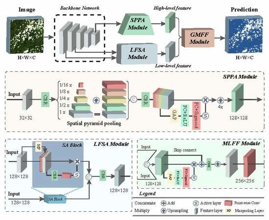
2. Methods
2.1. Backbone Network
2.2. Spatial Pyramid Pooling Attention Module
2.3. Low-Level Feature Spatial Attention Module
2.4. Gated Multilevel Feature Fusion Module
3. Experiments
3.1. Experimental Data
3.1.1. Dataset
3.1.2. Data Processing
3.2. Experiment Settings
3.2.1. Model Training and Prediction
3.2.2. Evaluation Metrics
4. Results
4.1. Evaluation of the MFGNet
4.2. Comparison Results
4.3. Example Scene and Performance
4.4. Efficiency Evaluation
5. Discussion
5.1. Method Advantage Analysis
5.2. Limitation Analysis
5.3. Extended Application
6. Conclusions and Future Developments
Author Contributions
Funding
Acknowledgments
Conflicts of Interest
References
- Yang, Y.; Li, H.; Du, Y.; Cao, B.; Liu, Q.; Sun, L.; Zhu, J.; Mo, F. A temperature and emissivity separation algortihm for chinese gaofen-5 satelltie data. In Proceedings of the 2018 IEEE International Geoscience and Remote Sensing Symposium(IGARSS 2018), Valencia, Spain, 22–27 July 2018; pp. 2543–2546. [Google Scholar]
- Liu, L.; Shang, K. Mineral information extraction based on gaofen-5′s thermal infrared data. Int. Arch. Photogramm. Remote Sens. Spat. Inf. Sci. 2018, XLII-3, 1157–1160. [Google Scholar] [CrossRef]
- Yu, J.C.; Yan, B.K. Efficient solution of large-scale domestic hyperspectral data processing and geological application. In Proceedings of the IEEE 2017 International Workshop on Remote Sensing with Intelligent Processing, Shanghai, China, 18–21 May 2017; pp. 1–4. [Google Scholar]
- King, M.D.; Platnick, S.; Menzel, W.P.; Ackerman, S.A.; Hubanks, P.A. Spatial and temporal distribution of clouds observed by modis onboard the terra and aqua satellites. IEEE Trans. Geosci. Remote Sens. 2013, 51, 3826–3852. [Google Scholar] [CrossRef]
- Irish, R.R.; Barker, J.L.; Goward, S.N.; Arvidson, T. Characterization of the landsat-7 etm+ automated cloud-cover assessment (acca) algorithm. Photogramm. Eng. Remote Sens. 2006, 72, 1179–1188. [Google Scholar] [CrossRef]
- Zhu, Z.; Woodcock, C.E. Object-based cloud and cloud shadow detection in landsat imagery. Remote Sens. Environ. 2012, 118, 83–94. [Google Scholar] [CrossRef]
- Zhu, Z.; Wang, S.; Woodcock, C.E. Improvement and expansion of the fmask algorithm: Cloud, cloud shadow, and snow detection for landsats 4–7, 8, and sentinel 2 images. Remote Sens. Environ. 2015, 159, 269–277. [Google Scholar] [CrossRef]
- Rossow, W.B.; Garder, L.C. Cloud detection using satellite measurements of infrared and visible radiances for isccp. J. Clim. 1993, 6, 2341–2369. [Google Scholar] [CrossRef]
- Gesell, G. An algorithm for snow and ice detection using avhrr data an extension to the apollo software package. Int. J. Remote Sens. 1989, 10, 897–905. [Google Scholar] [CrossRef]
- Stowe, L.; McClain, E.; Carey, R.; Pellegrino, P.; Gutman, G.; Davis, P.; Long, C.; Hart, S. Global distribution of cloud cover derived from noaa/avhrr operational satellite data. Adv. Space Res. 1991, 11, 51–54. [Google Scholar] [CrossRef]
- Qiu, S.; He, B.B.; Zhu, Z.; Liao, Z.M.; Quan, X.W. Improving fmask cloud and cloud shadow detection in mountainous area for landsats 4–8 images. Remote Sens. Environ. 2017, 199, 107–119. [Google Scholar] [CrossRef]
- Qiu, S.; Zhu, Z.; He, B. Fmask 4.0: Improved cloud and cloud shadow detection in landsats 4–8 and sentinel-2 imagery. Remote Sens. Environ. 2019, 231, 1–20. [Google Scholar] [CrossRef]
- Hagolle, O.; Huc, M.; Pascual, D.V.; Dedieu, G. A multi-temporal method for cloud detection, applied to formosat-2, venµs, landsat and sentinel-2 images. Remote Sens. Environ. 2010, 114, 1747–1755. [Google Scholar] [CrossRef]
- Zhu, Z.; Woodcock, C.E. Automated cloud, cloud shadow, and snow detection in multitemporal landsat data: An algorithm designed specifically for monitoring land cover change. Remote Sens. Environ. 2014, 152, 217–234. [Google Scholar] [CrossRef]
- Lin, C.H.; Lin, B.Y.; Lee, K.Y.; Chen, Y.C. Radiometric normalization and cloud detection of optical satellite images using invariant pixels. ISPRS J. Photogramm. Remote Sens. 2015, 106, 107–117. [Google Scholar] [CrossRef]
- Di Vittorio, A.V.; Emery, W.J. An automated, dynamic threshold cloud-masking algorithm for daytime avhrr images over land. IEEE Trans. Geosci. Remote Sens. 2002, 40, 1682–1694. [Google Scholar] [CrossRef]
- Sun, L.; Wei, J.; Wang, J.; Mi, X.; Guo, Y.; Lv, Y.; Yang, Y.; Gan, P.; Zhou, X.; Jia, C. A universal dynamic threshold cloud detection algorithm (udtcda) supported by a prior surface reflectance database. J. Geophys. Res. Atmos. 2016, 121, 7172–7196. [Google Scholar] [CrossRef]
- Luo, Y.; Trishchenko, A.P.; Khlopenkov, K.V. Developing clear-sky, cloud and cloud shadow mask for producing clear-sky composites at 250-meter spatial resolution for the seven modis land bands over canada and north america. Remote Sens. Environ. 2008, 112, 4167–4185. [Google Scholar] [CrossRef]
- Frantz, D.; Haß, E.; Uhl, A.; Stoffels, J.; Hill, J. Improvement of the fmask algorithm for sentinel-2 images: Separating clouds from bright surfaces based on parallax effects. Remote Sens. Environ. 2018, 215, 471–481. [Google Scholar] [CrossRef]
- Bian, J.; Li, A.; Liu, Q.; Huang, C. Cloud and snow discrimination for ccd images of HJ-1A/B constellation based on spectral signature and spatio-temporal context. Remote Sens. 2016, 8, 31. [Google Scholar] [CrossRef]
- Ge, S.L.; Dong, S.Y.; Sun, G.Y.; Du, Y.M.; Lin, Y. Cloud detection algorithm for images of visual and infrared multispectral imager. Aerosp. Shanghai 2019, 36, 204–208. [Google Scholar] [CrossRef]
- Zhan, Y.; Wang, J.; Shi, J.; Cheng, G.; Yao, L.; Sun, W. Distinguishing cloud and snow in satellite images via deep convolutional network. IEEE Geosci. Remote Sens. Lett. 2017, 14, 1785–1789. [Google Scholar] [CrossRef]
- Wang, L.; Chen, Y.; Tang, L.; Fan, R.; Yao, Y. Object-based convolutional neural networks for cloud and snow detection in high-resolution multispectral imagers. Water 2018, 10, 1666. [Google Scholar] [CrossRef]
- Oishi, Y.; Ishida, H.; Nakamura, R. A new landsat 8 cloud discrimination algorithm using thresholding tests. Int. J. Remote Sens. 2018, 39, 9113–9133. [Google Scholar] [CrossRef]
- Shao, Z.; Pan, Y.; Diao, C.; Cai, J. Cloud detection in remote sensing images based on multiscale features-convolutional neural network. IEEE Trans. Geosci. Remote Sens. 2019, 57, 4062–4076. [Google Scholar] [CrossRef]
- Hong, Y.; Hsu, K.L.; Sorooshian, S.; Gao, X. Precipitation estimation from remotely sensed imagery using an artificial neural network cloud classification system. J. Appl. Meteorol. 2004, 43, 1834–1853. [Google Scholar] [CrossRef]
- Hall, D.K.; Riggs, G.A.; Salomonson, V.V. Development of methods for mapping global snow cover using moderate resolution imaging spectroradiometer data. Remote Sens. Environ. 1995, 54, 127–140. [Google Scholar] [CrossRef]
- Ghasemian, N.; Akhoondzadeh, M. Introducing two random forest based methods for cloud detection in remote sensing images. Adv. Space Res. 2018, 62, 288–303. [Google Scholar] [CrossRef]
- Egli, S.; Thies, B.; Bendix, J. A hybrid approach for fog retrieval based on a combination of satellite and ground truth data. Remote Sens. 2018, 10, 628. [Google Scholar] [CrossRef]
- Lee, Y.; Wahba, G.; Ackerman, S.A. Cloud classification of satellite radiance data by multicategory support vector machines. J. Atmos. Ocean. Technol. 2004, 21, 159–169. [Google Scholar] [CrossRef]
- Ishida, H.; Oishi, Y.; Morita, K.; Moriwaki, K.; Nakajima, T.Y. Development of a support vector machine based cloud detection method for modis with the adjustability to various conditions. Remote Sens. Environ. 2018, 205, 390–407. [Google Scholar] [CrossRef]
- Li, Z.; Shen, H.; Cheng, Q.; Liu, Y.; You, S.; He, Z. Deep learning based cloud detection for medium and high resolution remote sensing images of different sensors. ISPRS J. Photogramm. Remote Sens. 2019, 150, 197–212. [Google Scholar] [CrossRef]
- Ma, L.; Liu, Y.; Zhang, X.; Ye, Y.; Yin, G.; Johnson, B.A. Deep learning in remote sensing applications: A meta-analysis and review. ISPRS J. Photogramm. Remote Sens. 2019, 152, 166–177. [Google Scholar] [CrossRef]
- Tsagkatakis, G.; Aidini, A.; Fotiadou, K.; Giannopoulos, M.; Pentari, A.; Tsakalides, P. Survey of deep-learning approaches for remote sensing observation enhancement. Sensors 2019, 19, 3929. [Google Scholar] [CrossRef] [PubMed]
- Zhang, L.; Li, H.; Shen, P.Y.; Zhu, G.M.; Song, J.; Shah, S.A.A.; Bennamoun, M.; Zhang, L. Improving Semantic Image Segmentation With a Probabilistic Superpixel-Based Dense Conditional Random Field. IEEE Access 2018, 6, 15297–15310. [Google Scholar] [CrossRef]
- Hegarat-Mascle, S.L.; Andre, C. Use of markov random fields for automatic cloud/shadow detection on high resolution optical images. ISPRS J. Photogramm. Remote Sens. 2009, 64, 351–366. [Google Scholar] [CrossRef]
- Chen, L.C.; Papandreou, G.; Kokkinos, I.; Murphy, K.; Yuille, A.L. Deeplab: Semantic image segmentation with deep convolutional nets, atrous convolution, and fully connected crfs. IEEE Trans. Pattern Anal. Mach. Intell. 2017, 40, 834–848. [Google Scholar] [CrossRef]
- Chai, D.; Newsam, S.; Zhang, H.K.; Qiu, Y.; Huang, J. Cloud and cloud shadow detection in landsat imagery based on deep convolutional neural networks. Remote Sens. Environ. 2019, 225, 307–316. [Google Scholar] [CrossRef]
- Mohajerani, S.; Saeedi, P. Cloud-net+: A cloud segmentation cnn for landsat 8 remote sensing imagery optimized with filtered jaccard loss function. arXiv 2020, arXiv:2001.08768. [Google Scholar]
- Yang, J.; Guo, J.; Yue, H.; Liu, Z.; Hu, H.; Li, K. Cdnet: Cnn-based cloud detection for remote sensing imagery. IEEE Trans. Geosci. Remote Sens. 2019, 57, 6195–6211. [Google Scholar] [CrossRef]
- Jeppesen, J.H.; Jacobsen, R.H.; Inceoglu, F.; Toftegaard, T.S. A cloud detection algorithm for satellite imagery based on deep learning. Remote Sens. Environ. 2019, 229, 247–259. [Google Scholar] [CrossRef]
- Drönner, J.; Korfhage, N.; Egli, S.; Mühling, M.; Thies, B.; Bendix, J.; Freisleben, B.; Seeger, B. Fast cloud segmentation using convolutional neural networks. Remote Sens. 2018, 10, 1782. [Google Scholar] [CrossRef]
- Liu, H.; Zeng, D.; Tian, Q. In Super-pixel cloud detection using hierarchical fusion cnn. In Proceedings of the 2018 IEEE Fourth International Conference on Multimedia Big Data, Xi’an, China, 13–16 September 2018; pp. 1–6. [Google Scholar]
- Morales, G.; Huamán, S.G.; Telles, J. In Cloud detection in high-resolution multispectral satellite imagery using deep learning. In Proceedings of the International Conference on Artificial Neural Networks, Kuala Lumpur, Malaysia, 21–23 November 2018; pp. 280–288. [Google Scholar]
- Guo, Z.S.; Li, C.H.; Wang, Z.M.; Kwok, E.; Wei, X. A cloud boundary detection scheme combined with aslic and cnn using zy-3, gf-1/2 satellite imagery. In Proceedings of the ISPRS Technical Commission III Midterm Symposium on “Developments, Technologies and Applications in Remote Sensing”, Beijing, China, 5–7 May 2018; pp. 699–702. [Google Scholar] [CrossRef]
- Zi, Y.; Xie, F.; Jiang, Z. A cloud detection method for landsat 8 images based on pcanet. Remote Sens. 2018, 10, 877. [Google Scholar] [CrossRef]
- Chen, Y.; Fan, R.; Bilal, M.; Yang, X.; Wang, J.; Li, W. Multilevel cloud detection for high-resolution remote sensing imagery using multiple convolutional neural networks. ISPRS Int. J. Geo-Inf. 2018, 7, 181. [Google Scholar] [CrossRef]
- Xie, F.; Shi, M.; Shi, Z.; Yin, J.; Zhao, D. Multilevel cloud detection in remote sensing images based on deep learning. IEEE J. Sel. Top. Appl. Earth Obs. Remote Sens. 2017, 10, 3631–3640. [Google Scholar] [CrossRef]
- Ronneberger, O.; Fischer, P.; Brox, T. In U-net: Convolutional networks for biomedical image segmentation. In Proceedings of the International Conference on Medical Image Computing and Computer-Assisted Intervention, Munich, Germany, 5–9 December 2015; pp. 234–241. [Google Scholar]
- Badrinarayanan, V.; Kendall, A.; SegNet, R.C. A deep convolutional encoder-decoder architecture for image segmentation. arXiv 2015, arXiv:1511.00561. [Google Scholar] [CrossRef] [PubMed]
- Simonyan, K.; Zisserman, A. Very deep convolutional networks for large-scale image recognition. arXiv 2014, arXiv:1409.1556. [Google Scholar]
- Hatamizadeh, A.; Terzopoulos, D.; Myronenko, A. Edge-gated cnns for volumetric semantic segmentation of medical images. arXiv 2020, arXiv:2002.04207. [Google Scholar]
- Takikawa, T.; Acuna, D.; Jampani, V.; Fidler, S. In Gated-scnn: Gated shape cnns for semantic segmentation. In Proceedings of the IEEE International Conference on Computer Vision, Seoul, Korea, 20–26 December 2019; pp. 5229–5238. [Google Scholar]
- Yu, C.; Wang, J.; Peng, C.; Gao, C.; Yu, G.; Sang, N. In Bisenet: Bilateral segmentation network for real-time semantic segmentation. In Proceedings of the European Conference on Computer Vision (ECCV 2018), Munich, Germany, 8–14 September 2018; pp. 325–341. [Google Scholar]
- Zhao, H.; Shi, J.; Qi, X.; Wang, X.; Jia, J. In Pyramid scene parsing network. In Proceedings of the IEEE Conference on Computer Vision and Pattern Recognition, Honolulu, HI, USA, 21–26 July 2017; pp. 2881–2890. [Google Scholar]
- Hu, J.; Shen, L.; Sun, G. In Squeeze-and-excitation networks. In Proceedings of the IEEE Conference on Computer Vision and Pattern Recognition, Salt Lake City, UT, USA, 18–22 June 2018; pp. 7132–7141. [Google Scholar]
- Xie, S.; Girshick, R.; Dollár, P.; Tu, Z.; He, K. In Aggregated residual transformations for deep neural networks. In Proceedings of the IEEE Conference on Computer Vision and Pattern Recognition, Honolulu, HI, USA, 21–26 July 2017; pp. 1492–1500. [Google Scholar]
- Zhang, Z.; Zhang, X.; Peng, C.; Xue, X.; Sun, J. In Exfuse: Enhancing feature fusion for semantic segmentation. In Proceedings of the European Conference on Computer Vision (ECCV 2018), Munich, Germany, 8–14 September 2018; pp. 269–284. [Google Scholar]
- Sandler, M.; Howard, A.; Zhu, M.; Zhmoginov, A.; Chen, L.C. In Mobilenetv2: Inverted residuals and linear bottlenecks. In Proceedings of the IEEE Conference on Computer Vision and Pattern Recognition, Salt Lake City, UT, USA, 18–22 June 2018; pp. 4510–4520. [Google Scholar]
- Howard, A.; Sandler, M.; Chu, G.; Chen, L.-C.; Chen, B.; Tan, M.; Wang, W.; Zhu, Y.; Pang, R.; Vasudevan, V. In Searching for mobilenetv3. In Proceedings of the IEEE International Conference on Computer Vision, Seoul, Korea, 20–26 December 2019; pp. 1314–1324. [Google Scholar]
- Chollet, F. In Xception: Deep learning with depthwise separable convolutions. In Proceedings of the IEEE Conference on Computer Vision and Pattern Recognition, Honolulu, HI, USA, 21–26 July 2017; pp. 1251–1258. [Google Scholar]
- Chen, L.-C.; Zhu, Y.; Papandreou, G.; Schroff, F.; Adam, H. In Encoder-decoder with atrous separable convolution for semantic image segmentation. In Proceedings of the European Conference on Computer Vision (ECCV 2018), Munich, Germany, 8–14 September 2018; pp. 801–818. [Google Scholar]
- Kingma, D.P.; Ba, J. Adam: A method for stochastic optimization. arXiv 2014, arXiv:1412.6980. [Google Scholar]
- Glorot, X.; Bengio, Y. In Understanding the difficulty of training deep feedforward neural networks. In Proceedings of the Thirteenth International Conference on Artificial Intelligence and Statistics, Sardinia, Italy, 13–15 May 2010; pp. 249–256. [Google Scholar]
- Sokolova, M.; Lapalme, G. A systematic analysis of performance measures for classification tasks. Inf. Process. Manag. 2009, 45, 427–437. [Google Scholar] [CrossRef]


| Authors | Date | Pixel-/Objectwise | Method | CNN Structure |
|---|---|---|---|---|
| Sorour Mohajerani et al. [39] | 2020 | Pixel | Cloud-Net+ [39] | U-shape + Branches |
| Zhiwei Li et al. [31] | 2019 | Pixel | MSCFF [31] | U-shape + Branches |
| Jingyu Yang et al. [40] | 2019 | Pixel | CDnet [40] | Multi-scale |
| Jacob Hobroe Jeppesen et al. [41] | 2019 | Pixel | RS-Net [41] | U-shape |
| Dengfeng Chai et al. [38] | 2019 | Pixel | Modified SegNet [38] | U-shape |
| Zhengfeng Shao et al. [25] | 2019 | Pixel | MF-CNN [25] | Multi-branch |
| Yongjie Zhan et al. [22] | 2019 | Pixel | FCN [22] | Linear stack + Branches |
| Johannes Dronner et al. [42] | 2018 | Pixel | CS-CNN [42] | U-shape |
| Han Liu et al. [43] | 2018 | Object | SLIC+HFCNN+ Deep Forest [43] | Linear stack |
| Giorgio Morales et al. [44] | 2018 | Object | ASLIC+CNN [44] | Linear stack |
| Lei Wang et al. [23] | 2018 | Object | ASLIC+CNN [23] | Dual-branch |
| Zhengsheng Guo et al. [45] | 2018 | Object | ASLIC+CNN [45] | Dual-branch |
| Yue Zi et al. [46] | 2018 | Object | SLIC+PCANet [46] | Dual-branch |
| Yang Chen et al. [47] | 2018 | Object | SLIC+MCNNNs [47] | Multi-branch |
| Fengying Xie et al. [48] | 2017 | Object | SLIC+Multi-level CNN [48] | Dual-branch |
| Stage | Input | Output | Operator | Filters | SE | Stride | Dilation Rate |
|---|---|---|---|---|---|---|---|
| 1 | 256 | 256 | CBR | 32 | 1 | 1 | |
| 256 | 256 | CBR | 32 | 1 | 1 | ||
| 256 | 128 | CBR | 64 | 2 | 1 | ||
| 2 | 128 | 128 | RCB | 64 | 1 | 1 | |
| 128 | 128 | ICB | 64 | yes | 1 | 1 | |
| 128 | 128 | ICB | 64 | yes | 1 | 1 | |
| 3 | 128 | 64 | RCB | 128 | 2 | 2 | |
| 64 | 64 | ICB | 128 | yes | 1 | 2 | |
| 64 | 64 | ICB | 128 | yes | 1 | 2 | |
| 64 | 64 | ICB | 128 | yes | 1 | 2 | |
| 4 | 64 | 32 | RCB | 256 | 2 | 4 | |
| 32 | 32 | ICB | 256 | yes | 1 | 4 | |
| 32 | 32 | ICB | 256 | yes | 1 | 4 | |
| 32 | 32 | ICB | 256 | yes | 1 | 4 | |
| 32 | 32 | ICB | 256 | yes | 1 | 4 | |
| 32 | 32 | ICB | 256 | yes | 1 | 4 | |
| 5 | 32 | 32 | RCB | 512 | 1 | 5 | |
| 32 | 32 | ICB | 512 | yes | 1 | 5 | |
| 32 | 32 | ICB | 512 | yes | 1 | 5 |
| Model | Accuracy | Precision | Recall | F1 Score | IoU |
|---|---|---|---|---|---|
| FCN8 | 0.96 | 0.96 | 0.80 | 0.83 | 0.73 |
| SegNet | 0.97 | 0.97 | 0.87 | 0.88 | 0.80 |
| PSPNet | 0.96 | 0.96 | 0.81 | 0.84 | 0.74 |
| BiSeNet | 0.97 | 0.97 | 0.88 | 0.89 | 0.81 |
| MFGNet | 0.99 | 0.99 | 0.93 | 0.94 | 0.90 |
| Model | MFLOPs | #Params (106) | Model Size (mb) | Time Cost (Seconds/Scene) |
|---|---|---|---|---|
| FCN8 | 67.18 | 33.60 | 384 | 3.59 |
| SegNet | 35.74 | 10.19 | 116 | 3.75 |
| PSPNet | 44.01 | 21.97 | 251 | 9.90 |
| BiSeNet | 52.53 | 26.19 | 299 | 7.76 |
| MFGNet | 15.72 | 7.83 | 90.5 | 9.87 |
© 2020 by the authors. Licensee MDPI, Basel, Switzerland. This article is an open access article distributed under the terms and conditions of the Creative Commons Attribution (CC BY) license (http://creativecommons.org/licenses/by/4.0/).
Share and Cite
Yu, J.; Li, Y.; Zheng, X.; Zhong, Y.; He, P. An Effective Cloud Detection Method for Gaofen-5 Images via Deep Learning. Remote Sens. 2020, 12, 2106. https://doi.org/10.3390/rs12132106
Yu J, Li Y, Zheng X, Zhong Y, He P. An Effective Cloud Detection Method for Gaofen-5 Images via Deep Learning. Remote Sensing. 2020; 12(13):2106. https://doi.org/10.3390/rs12132106
Chicago/Turabian StyleYu, Junchuan, Yichuan Li, Xiangxiang Zheng, Yufeng Zhong, and Peng He. 2020. "An Effective Cloud Detection Method for Gaofen-5 Images via Deep Learning" Remote Sensing 12, no. 13: 2106. https://doi.org/10.3390/rs12132106
APA StyleYu, J., Li, Y., Zheng, X., Zhong, Y., & He, P. (2020). An Effective Cloud Detection Method for Gaofen-5 Images via Deep Learning. Remote Sensing, 12(13), 2106. https://doi.org/10.3390/rs12132106