Abstract
Adversarial training has demonstrated advanced capabilities for generating image models. In this paper, we propose a deep neural network, named a classified adversarial network (CAN), for multi-spectral image change detection. This network is based on generative adversarial networks (GANs). The generator captures the distribution of the bitemporal multi-spectral image data and transforms it into change detection results, and these change detection results (as the fake data) are input into the discriminator to train the discriminator. The results obtained by pre-classification are also input into the discriminator as the real data. The adversarial training can facilitate the generator learning the transformation from a bitemporal image to a change map. When the generator is trained well, the generator has the ability to generate the final result. The bitemporal multi-spectral images are input into the generator, and then the final change detection results are obtained from the generator. The proposed method is completely unsupervised, and we only need to input the preprocessed data that were obtained from the pre-classification and training sample selection. Through adversarial training, the generator can better learn the relationship between the bitemporal multi-spectral image data and the corresponding labels. Finally, the well-trained generator can be applied to process the raw bitemporal multi-spectral images to obtain the final change map (CM). The effectiveness and robustness of the proposed method were verified by the experimental results on the real high-resolution multi-spectral image data sets.
1. Introduction
With the advances of science and technology, the ability of human beings to develop resources and transform nature has been continuously enhanced. Changes in the natural world and various human activities are changing the surface landscape and its land use forms every day. The rapid growth of the world’s population and the continuous acceleration of urbanization have accelerated the speed of this change. Land cover change research has become the focus of researchers [1,2,3]. Due to the characteristics of remote sensing technology, including real-time, fast, wide coverage, multi-spectral, periodicity, etc. [4], this technology has become the main technical means of change detection [5,6]. Remote sensing image change detection has become an important branch in remote sensing applications.
In recent years, remote sensing change detection has become a research hotspot, and has been widely applied in many fields, including disaster assessment [7], environmental monitoring [8], and urban expansion [9]. Remote sensing change detection could identify differences between images acquired at different times in identical geographic areas [10,11]. A multi-spectral image has abundant spectral information. With developed earth observation technology, we could obtain more and more multi-spectral images for remote sensing change detection; thus, we introduce a novel change detection method in multi-spectral remote sensing imagery.
Traditional change detection methods can be divided into three steps [7]. The first step is image pre-processing, which makes the images as comparable as possible. In this step, co-registration [12] and denoising [13] are widely used for image pre-processing. The second step is the generation of the difference image (DI). In this step, change vector analysis (CVA) [14], based on the Euclidean distance between the pixels, is widely used to generate the difference image. As this method must take all the spectral data into account and the multi-spectral image has many spectra, this could cause many calculations. Therefore, principal component analysis (PCA) is typically used for the feature selection of multi-spectral images [15,16,17], and the most representative features are selected for change detection. However, there are some shortcomings in this method, such as the unbalanced data, which could influence this method. The third step is classification, which is able to distinguish pixels into changed and unchanged. In this step, classification problems can be divided into unsupervised methods and supervised methods. As the unsupervised methods do not need to collect and label the ground truth [18,19], this is widely applied in remote sensing change detection, such as thresholding [20,21] and clustering strategies [22,23].
In recent years, many traditional methods were proposed for remote sensing image change detection and have achieved great performance. Lv et al. [24] combined k-means clustering and adaptive majority voting techniques [25] for remote sensing image change detection, and this method demonstrated better detection accuracy. Zhong et al. [26] proposed a multifeature probabilistic ensemble conditional random field model, which comprehensively considers the spectral characteristics of single pixels and the interactions between domain pixels. Liu et al. [27] proposed an unsupervised change detection method based on a histogram threshold using a Gaussian mixture model. Wan et al. [28] proposed a change detection method based on sorted histograms.
Although these methods have achieved great performance, they have some disadvantages; the unsupervised methods cannot identify the detailed change information, especially when changed and unchanged features overlap or inaccurately model their statistical distributions, or the unsupervised methods could produce poor results. This situation would become worse as the spatial resolution increases. Supervised methods [29,30] mainly use prior information to train the classifier that can classify pixels into changed and unchanged. However, there is great difficulty in labeling the training data. Supervised and unsupervised methods mainly rely on the hand-crafted feature representation; thereby, the performance of modeling complex high-level change information is poor. Multi-spectral images have much spectral information, which means that these traditional methods face many challenges [31]. Thus, it is necessary to explore new methods for multi-spectral image change detection.
Deep learning has been widely applied in remote sensing image processing tasks and has achieved excellent performance [32,33,34]. With the continuous development of deep neural networks, such as AlexNet [35], VGGNet [36], and GoogleNet [37], remote sensing image change detection methods based on deep learning have achieved great success. The change detection methods based on deep learning could be divided into two steps. First, the bitemporal images are handled by traditional methods, like CVA-based [38] and PCA-based [39] approaches, to obtain the initial change detection results. Then, suitable samples are selected from the initial results as the training set, and these samples are fed into the deep neural network to train the network. When the network is trained well, the test images are input into the neural network to obtain the final change detection results [40,41].
Lin et al. [42] adopted an end-to-end bilinear convolutional neural network to detect changes. Liu et al. [43] proposed a deep siamese convolutional network model with dual task constraints that contained three subnets for change detection. Zhang et al. [44] proposed a two-stage object-based deep learning method for multi-temporal Synthetic Aperture Radar (SAR) image change detection. Lu et al. [45] proposed a spectral–spatial joint learning network considering both spectral and spatial information. Although the change detection methods based on deep learning achieved considerable detection results, it is very difficult to produce labeled data; thus, unsupervised methods typically perform better than supervised methods [46].
As it is difficult to obtain sufficiently reliable labeled samples to train a network, the deep-learning-based methods using a single deep neural network cannot adequately learn the concept of changed and unchanged pixels. The generative adversarial networks (GANs) have become a research hotspot and have demonstrated advanced results for image generation models [47,48]. The specific network structure for GANs can be set according to the actual application, rather than a fixed structure. M. Gong et al. explored the GAN-based change detection method (GAND) as multi-spectral change detection [49]. In the method, a better difference image (DI) can be obtained by a generator and, then, can be analyzed with a clustering algorithm to obtain the change detection result. However, the performance of this approach is still affected by the clustering algorithm.
Thus, we developed a new classified adversarial network (CAN) based on GANs for multi-spectral change detection. By adversarial training, a generator can better learn the relationship between the bitemporal multi-spectral image data and the corresponding labels. Finally, the well-trained generator can be applied to process the raw bitemporal multi-spectral images, and the final change map (CM) can be generated. For the whole process, this change detection method is completely unsupervised and can meet specific application needs.
In this paper, we propose a classified adversarial network for multi-spectral remote sensing image change detection. First, the method based CVA was used to generate the initial CM, and then the training sample selection method was used to select the training sample. Secondly, the selected sample was input into the classified adversarial network to train this network. When the discriminator is unable to identify the generated fake data, the data generated by the generator is very similar to the real data. Finally, the generator can output the final change detection result. The contributions of this paper are summarized as follows:
(1) This paper proposed the method named CAN to solve change detection in multi-spectral remote sensing images. Experimental results on the real multi-spectral remote sensing images demonstrated that the proposed CAN trained by unlabeled data and a small amount of labeled data can achieve better performance.
(2) We used a sample selection method based on neighborhood information to select training samples, which made the selected training samples more reliable.
(3) The performance of the classified adversarial network was not affected by the clustering algorithm. The data generated by the generator can be directly used as the final result, and does not need to be processed by the clustering algorithm.
2. Methodology
In this section, we will introduce the procedure of CAN, which includes generative adversarial networks, training sample selection, network establishment, and network training. Figure 1 shows the framework of classified adversarial networks for multi-spectral remote sensing image change detection.
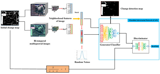
Figure 1.
Flowchart of the classified adversarial network (CAN)-based method for remote sensing image change detection. First, the initial change detection result is obtained using a change vector analysis (CVA)-based method. Then, the reliable, labeled data can be selected according the initial result. Adding noise into the labeled data is regarded as fake data. Labeled data and fake data are used to train the CAN, and the discriminator is used to judge whether the output of the classifier is reliable. Finally, bitemporal multi-spectral remote sensing images are fed into the classifier when it is trained well to obtain the final change map (CM).
2.1. Generative Adversarial Networks
The GANs were proposed by Goodfellow et al. in 2014 [50]. The main structure of GANs includes a G (Generator) and a D (Discriminator). During the training process, the generator gradually becomes stronger in generating realistic images, and the discriminator gradually becomes stronger in the ability to distinguish these images. When the discriminator is no longer able to distinguish between real and fake pictures, the training process is balanced. GANs training is in a state of confrontation, and follows the objective function:
In Equation (1), the x represents real data, z represents the additional noise, and represents the empirical estimate of the expected value of the probability. After continuous adversarial training, the skills of the G (Generator) continue to improve, and finally deceive the discriminator D (Discriminator). Discriminator D improves its own discrimination ability, and finally can accurately judge the fake data. When D cannot identify the fake data generated by G, the data generated by G is very similar to the target data.
2.2. Pre-Classification
Before the selection of training samples, we obtained the initial results using a traditional method. The method based on change vector analysis (CVA) is widely used in change detection, and was used to obtain the initial result for the selection. The two multi-spectral images, registered as and , correspond to different times, and , over the same area. The DI between these two images was obtained by the CVA. The Otsu algorithm is a widely used thresholding approach that is easy to apply and performs well [51]. The Otsu algorithm processes the difference image (DI) obtained by CVA, which gains the initial change map (CM) by classifying the pixels of the DI into changed and unchanged classes. Figure 2 shows the flowchart of generating the initial change map.
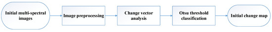
Figure 2.
Flowchart of the CVA-based method for generating the initial change map.
Figure 3, Figure 4 and Figure 5 show the change maps obtained with the CVA-based method and the real results. In Figure 3, compared with the real results, the change maps obtained with the CVA-based method have many white noise points, and some unchanged regions that are incorrectly classified into changed areas. In Figure 4 and Figure 5, due to the geographical environment being more complicated and the pixel value of the area where the image changes not being obvious, the change map obtained with the CVA-based method has a great deal of false detection. Compared with reference images, the change maps obtained with the CVA-based method were not satisfactory. Therefore, the sample selection approach was used to select samples to obtain better results.
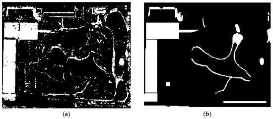
Figure 3.
(a) The change map obtained with the CVA-based method in the Yandu Village data set. (b) The reference image of the Yandu Village data set.
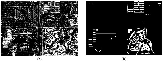
Figure 4.
(a) The change map obtained with the CVA-based method in the Minfeng data set. (b) The reference image of the Minfeng data set.
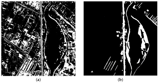
Figure 5.
(a) The change map obtained with the CVA-based method in the Hongqi Canal data set. (b) The reference image of the Hongqi Canal data set.
2.3. Training Samples Selection
The results obtained by the CVA-based method cannot be directly used to train the network. From the pre-processed results, we selected the sample with the highest probability of being classified correctly. For the initial change detection result, we used neighborhood-based criteria to choose the training samples [40].
where the neighborhood of the pixel is in the . In the initial change map, the pixel is at position (i, j), and the is a neighborhood centered on . is the number of pixels in the neighborhood where the label is the same as . is the size of the neighborhood. If the pixel satisfies the condition in Equation (2), it will be selected as the training sample. Figure 6 shows the impact of the threshold on the accuracy of the selected samples. When the threshold is set to 1, the accuracy of selected samples is the highest. Therefore, in this paper, the threshold was set to 1. Figure 7 shows the examples of training samples selected under different thresholds in the Yandu Village data set. When the threshold was set to 1, the size of training sample was the smallest.
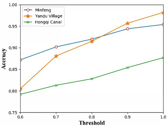
Figure 6.
The impact of the threshold on the accuracy of the selected samples.
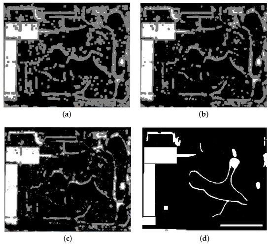
Figure 7.
Examples of the training samples selected under different thresholds in the Yandu Village data set. The white region is the selected changed pixels, the black region is the selected unchanged pixels, and the gray region is the not-selected pixels. (a) The threshold is 1. (b) The threshold is 0.9. (c) The threshold is 0.8. (d) The reference image of the Yandu Village data set.
2.4. Network Establishment
The CAN includes a G and a D, in which G is not only a generator, but also a classifier. The multi-spectral image data of different phases are fed into G, and their corresponding outputs are the categories of the pixels, which are changed or unchanged. The results of G are fed into D as the fake data. In addition, the results obtained by pre-classification are entered into D as the real data. In the CAN, the neighborhood features of the image pixels are fed into G to make use of the spatial information and robust local features of the pixels [41]. The CAN can be built by G and D above, where G and D are composed of multi-layer perceptrons. G is composed of , and D consists of in the proposed framework. The indicates the neighborhood size of pixels and N indicates the number of spectrums. For each pixel location, the neighborhood features of the two phases are connected to the final feature, so the input dimension of G is .
2.5. Network Training
All the training samples obtained from the pre-classification are used for training the CAN, and the training process follows the objective function below:
where
x is the “real” change map, named as the initial change detction result by pre-classification, and y is the bitemporal multi-spectral pixel data and noise-added pixel data. The first term of aims to increase the probability that pixels belong to the real class, and the second term of aims to force D to distinguish between the real data and fake data generated by G, to increase the probability that the generated data belongs to the fake class. G converts the bitemporal multi-spectral data into the data that are similar to the “real” CM. The first term of aims to decrease the probability that generated data belongs to the fake class. The second term of aims to decrease the distance between the generated data and real data to generate data that are closer to the real data. The previous methods have demonstrated the advantages of and distance for the GANs. We applied the distance instead of because brings less blurs [47,48]. The controls the weight of in the objective function in Equation (4).
The specific training process of the CAN is stated as follows. First, the parameters of G and D that contain weights and biases are randomly initialized. Then, G and D are trained with the random gradient descent algorithm. D is trained by optimizing Equation (3) with training samples when G is fixed. This is followed by optimizing Equation (4) to train G when D is fixed. Thus, G and D are alternately trained like this until Equation (3) is convergent. Through the adversarial training between G and D, G can learn the transformation from bitemporal images to the CM.
The output layer of G is a sigmoid function, whose value represents the probability that the pixel belongs to the changed or unchanged class. We can obtain the final change detection result according to the output of G. The behavior of the change map over the evolution of the training process is shown in Figure 8. In Figure 8, we chose four representative change maps generated by G in the Minfeng data set, from which we found that the data generated by G was increasingly similar to the real data. Figure 9 shows the losses of the Generator and Discriminator during the training in the Minfeng data set. With the continuous alternating training of G and D, the ability of D to distinguish the fake and real data becomes stronger and stronger, and the ability of G to capture the data distribution also becomes stronger.
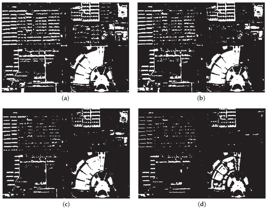
Figure 8.
The behavior of the change map over the evolution of the training process. (a) The output of G in the first iteration (FP:44389; FN:4893; OE:49282; KC:0.3617; :0.4355). (b) The output of G in the tenth iteration (FP:35905; FN:4945; OE:40850; KC:0.4167; :0.4814). (c) The output of G in the twentieth iteration (FP:22824; FN:6182; OE:29006; KC:0.4998; :0.5499). (d) The output of G in the final iteration (FP:9772; FN:7381; OE:17153; KC:0.6272; :0.6583).
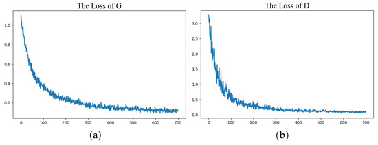
Figure 9.
The losses of the Generator and Discriminator during training. (a) The loss of G. (b) The loss of D.
As the selected pixels and the not-selected pixels are from the same data set, there is similarity between the features. Therefore, the classifier is used to process the not-selected pixels and classify them as changed and unchanged. The entire network can not only be applied to the not-selected pixels but can also reduce the interference of the error information in the training samples to the network performance. The training procedure of the CAN is summarized in Algorithm 1.
| Algorithm 1 The procedure of the CAN. |
| Input: A pair of initial images Output: Final change map (CM) 1. Obtain the difference image (DI) by change vector analysis (CVA). 2. Use Otsu to divide the pixels in the differential image into changed and unchanged, and obtain the initial change map (CM). 3. Use the sample selection algorithm to select training samples in the initial change map. 4. The parameters of G and D randomly initialize. 5. Fix network G, and update the parameters of D by optimizing Equation (3). 6. Fix network D, update the parameters of G by optimizing Equation (4). 7. Alternately perform step 5 and step 6 until Equation (3) is convergent. Return: The final classification result (changed or unchanged) |
3. Experimental Study
In order to verify the effectiveness of our proposed method from multiple aspects, we selected five contrast algorithms to experiment on three multi-spectral remote sensing data sets. The first was the CVA-based method. This method first used change vector analysis (CVA) to obtain the difference images (DI), and then Otsu was used to obtain the final result. The second was a PCA-based method [52]. Principal component analysis (PCA) is typically used for feature selection of multi-spectral images, and the most representative features are selected for change detection. The third was a deep neural network (DNN)-based method, the network structure of the DNN-based method was the same as the G (Generator), and we used labeled data to train this network. The forth was a GAN-based method (GAND) [53]. For the GAN-based method, we selected the best combination in the GAND as a comparative method by training the network with the same data set. The fifth was based on iterative reweighted multivariate change detection (IR-MAD) and GAN [53]. IR-MAD repeatedly assigns different weights to observations until they converge and are more stable.
3.1. Data Sets Description
We selected three representative data sets to verify the proposed method. These three data sets were the Yandu Village data set, Minfeng data set, and Hongqi Canal data set, as shown in Figure 10, Figure 11 and Figure 12. The images on the three data sets had four bands (R, G, B, and NIR). The details of the data sets we used are introduced in Table 1. The false negative (FN) indicates that changed pixels are mistakenly detected as unchanged pixels. The false positive (FP) indicates that unchanged pixels are incorrectly detected as changed pixels. The true positive (TP) indicates the changed pixels that are correctly detected. The true negative indicates the unchanged pixels that are correctly detected. The false positive (FP), false negative (FN), overall error (OE), kappa coefficient (KC), and first error measure can be used to assess the change detection method [54]. Where
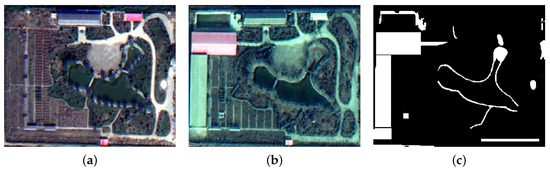
Figure 10.
The Yandu Village data set. (a) Image acquired on 19 September 2012. (b) Image acquired on 10 February 2015. (c) Reference image.
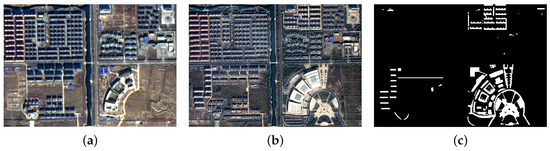
Figure 11.
The Minfeng data set. (a) Image acquired on 9 December 2013. (b) Image acquired on 16 October 2015. (c) Reference image.
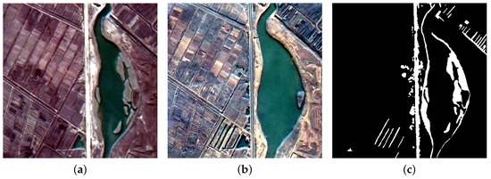
Figure 12.
The Hongqi Canal data set. (a) Image acquired on 9 December 2013. (b) Image acquired on 16 October 2015. (c) Reference image.

Table 1.
Details of the data sets we used.
In Equation (7), represents the percentage of the overall accuracy, and represents the ratio of expected agreement, as follows:
3.2. Parameter Setting
3.2.1. Effects of Parameter
In this paper, the represents the size of the neighborhood. The value of determines how much neighborhood information is included: a larger means richer neighborhood information. Less neighborhood information will make it more difficult to learn the inherent features of the image. Conversely, sufficient feature information can give the network sufficient feature information for training but could generate redundant information. We set as 3, 5, 7, and 9 to obtain change detection results with the proposed method. Figure 13 shows the relationship between KC and and the in the three data sets. According to the line chart, when was set to 5, the change detection results were satisfactory, and the best performance was obtained on three real image data sets. The choice of the size of the neighborhood depends on the type of observed scene; the optimal sizes of the neighborhood will be different. In practical applications, should be set accordingly for the different observed scenes.
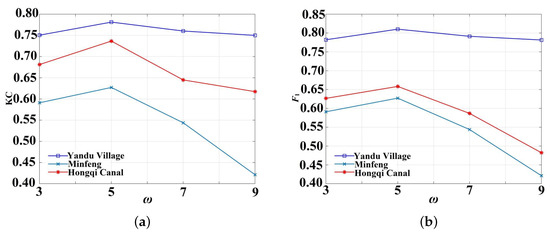
Figure 13.
The impact of on the change detection results. (a) The impact of on KC. (b) The impact of on .
3.2.2. Effects of Parameter
In this paper, the was set from 0 to 100 to obtain the change detection results with the proposed method. The KC and OE became stable when was greater than 15. Figure 14 shows the relationship between KC and OE and the . When was 0, the CM generated by G was different from the real data, and CAN had poor performance on all three data sets. When the was 1, CAN achieved the best performance on the Minfeng and Hongqi Canal data sets. This is because facilitates G to generate data similar to the real data so that more image data are correctly classified into the changed or unchanged classes. When was greater than 1, the KC started to drop, OE started to increase and gradually stabilize when was greater than 7 for these two data sets. The CAN was affected by the noise information in multi-spectral images when was too large so that G could not effectively transform the bitemporal image data into the CM. CAN maintained good performance on the Yandu Village data set when was equal to or greater than 1. Therefore, it was reliable for the three data sets to set to 1 through the above analysis. In practical applications, we should set the value of according to the different observed scenes.
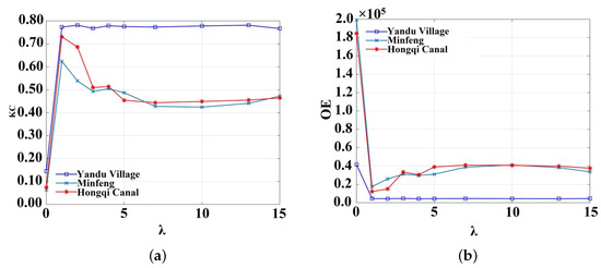
Figure 14.
The impact of on the change detection results. (a) The impact of on KC. (b) The impact of on .
3.2.3. Results on the Yandu Village Data Set
Figure 15 shows the final change map of the Yandu Village data set by various change detection methods. As shown in Figure 15a, the change map obtained with the CVA-based method contains a great deal of noise, and there are a large number of pixels that were erroneously detected in the results obtained by the CVA-based method. Therefore, the change map obtained by CVA-based method still requires improvement. Figure 15b shows the change map gained with the PCA-based method. There is also a greta deal of noise, and some unchanged regions are incorrectly classified into changed areas, which is still unsatisfactory. Figure 15c shows the results obtained by the DNN-based method. All of the selected samples were used to train the DNN. Compared with the CVA-based method and PCA-based method, the results of change detection were greatly improved.
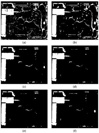
Figure 15.
CMs for the Yandu Village data set produced by various methods. (a) CVA. (b) Principal component analysis (PCA). (c) Deep neural network (DNN). (d) Generative adversarial network (GAN)-based method (GAND). (e) Iterative reweighted multivariate change detection (IR-MAD)+GAN. (f) CAN.
This result demonstrates the powerful learning ability of the DNN. Figure 15d,e shows the results obtained by GAND and IR-MAD+GAN. When there were less noise points in the changed area, this method demonstrated good performance. However, when there were many noise points in the changed area, GAND incorrectly detected some of the changed areas into unchanged areas. CAN could better learn the distribution of the image and transform it into a CM. Thus, CAN could detect more changed areas in comparison with GAND; the CM is shown in Figure 15f. Quantitative analysis for various methods is listed in Table 2. Compared with other methods, the CAN we proposed had the best performance (i.e., the KC was 0.7813, and the was 0.8102).
Table 2.
Evaluation of the experimental results on the Yandu Village data set. False positive (FP), false negative (FN), overall error (OE), kappa coefficient (KC), and first error measure .
3.2.4. Results on the Minfeng Data Set
Changes in the MinFeng data set were mainly changes in buildings in the process of urbanization, and it was more difficult to detect changes in this complex geographic environment. As shown in Figure 16a,b, the CMs generated by the CVA-based method and the CVA-based method had many white noise points and some changed areas were not accurately detected. DNN had poor performance on the Minfeng data set because the training data of the Minfeng data set included many inaccurate datapoints; its CM is shown in Figure 16c. For these two images, as shown in Figure 16d, GAND was able to obtain a more accurate DI, and was able to identify most of the changed areas. Figure 16e shows the results obtained by IR-MAD+GAN. IR-MAD+GNN had poor performance on the Minfeng data set because the IR-MAD incorrectly classified residential areas (upper left corner) as changed areas. Figure 16f shows the CM obtained by CAN, CAN could gain good performance because the G could better learn the relationship between the image data and the CM. Furthermore, according to Table 3, the CAN we proposed had the best performance (i.e., the KC was 0.6272, and the was 0.6583).
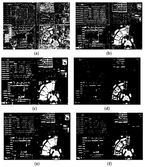
Figure 16.
CMs for the Minfeng data set produced by various methods. (a) CVA. (b) PCA. (c) DNN. (d) GAND. (e) IR-MAD+GAN. (f) CAN.
Table 3.
Evaluation of the experimental results on the Minfeng data set.
3.2.5. Results on the Hongqi Canal Data Set
Changes in the Hongqi Canal data set were mainly changes in the river and land near Xijiu Village. Figure 17a shows the results obtained with the CVA-based method. The CM generated by the CVA-based method had many unchanged regions that were incorrectly detected as changed regions. As shown in Figure 17b, the CM generated by the PCA-based method had some white noise points. Some small changed areas could not be recognized. For example, changes in the lower left corner were not detected. Figure 17c shows the results obtained with the DNN-based method. Compared with the CVA-based method and PCA-based method, the results obtained by the DNN-based method had less noise points, and the small changed area was detected.
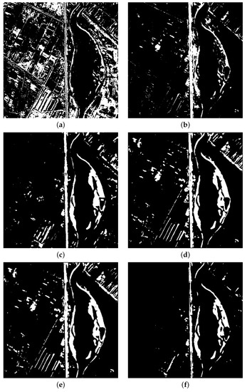
Figure 17.
CMs for the Hongqi data set produced by various methods. (a) CVA. (b) PCA. (c) DNN. (d) GAND. (e) IR-MAD+GAN. (f) CAN.
Figure 17d represents the change detection result of the GAND-based method on this data set. The GAND-based method detected a number of changed areas with some white noise points. Although it achieved a better DI, The performance of the clustering algorithm limited the performance of the GAND-based method. As shown in Figure 17e, the CM generated by IR-MAD+GAN had more pixels that were erroneously detected. The CM obtained by CAN with less noise points is shown in Figure 17f, and could detect major changed areas. The quantitative analysis for various methods is listed in Table 4. Compared with other methods, the CAN we proposed had the best performance (i.e., the KC was 0.7366, and the was 0.7572).
Table 4.
Evaluation of the experimental results on the Hongqi Canal data set.
4. Conclusions
In this paper, a classified adversarial network (CAN) was established for multi-spectral image change detection. The initial change detection results were obtained by pre-classification. Multi-spectral image data were input into the generator and then converted into data similar to the initial change detection results. By adversarial training, the generator could classify the changed pixels and unchanged pixels. When the generator was trained well, the generator had the ability to divide the pixels into two categories: changed and unchanged, and the generator could output the final change map. Although the CAN requires trained samples to be provided through pre-classification, pre-classification only needs to filter the samples by adding constraints, and there is no manual intervention in this process. Therefore, the proposed method is completely unsupervised in the whole process. From the experiments on real multi-spectral image data sets with high resolution, our qualitative and quantitative analysis demonstrated the effectiveness and advantages of the proposed method for multi-spectral image change detection.
Author Contributions
Y.W. and Z.B. conceived and designed the experiments; Y.Y. and Z.B. performed the experiments; Q.M. and M.G. analyzed the data; W.M., M.G. and Q.M. contributed materials; Z.B. wrote the paper. Y.W. supervised the study and reviewed this paper. All authors have read and agreed to the published version of the manuscript.
Funding
This work was supported in part by the National Natural Science Foundation of China under Grant 61702392, and the Natural Science Basic Research Program of Shaanxi (Program No. 2019JQ-189).
Conflicts of Interest
The authors declare no conflict of interest.
References
- Jin, S.; Yang, L.; Zhu, Z.; Homer, C. A land cover change detection and classification protocol for updating Alaska NLCD 2001 to 2011. Remote Sens. Environ. 2017, 195, 44–55. [Google Scholar] [CrossRef]
- Lyu, H.; Lu, H.; Mou, L. Learning a transferable change rule from a recurrent neural network for land cover change detection. Remote Sens. 2016, 8, 506. [Google Scholar] [CrossRef]
- Polykretis, C.; Grillakis, M.G.; Alexakis, D.D. Exploring the impact of various spectral indices on land cover change detection using change vector analysis: A case study of Crete Island, Greece. Remote Sens. 2020, 12, 319. [Google Scholar] [CrossRef]
- Zhao, S.; Wang, Q.; Li, Y.; Liu, S.; Wang, Z.; Zhu, L.; Wang, Z. An overview of satellite remote sensing technology used in China’s environmental protection. Earth Sci. Inform. 2017, 10, 137–148. [Google Scholar] [CrossRef]
- Sofina, N.; Ehlers, M. Building change detection using high resolution remotely sensed data and GIS. IEEE J. Sel. Top. Appl. Earth Obs. Remote Sens. 2016, 9, 3430–3438. [Google Scholar] [CrossRef]
- López-Fandiño, J.; Heras, D.B.; Argüello, F.; Dalla Mura, M. GPU framework for change detection in multitemporal hyperspectral images. Int. J. Parallel Program. 2019, 47, 272–292. [Google Scholar] [CrossRef]
- Aminikhanghahi, S.; Cook, D.J. A survey of methods for time series change point detection. Knowl. Inf. Syst. 2017, 51, 339–367. [Google Scholar] [CrossRef] [PubMed]
- Tan, K.; Zhang, Y.; Wang, X.; Chen, Y. Object-based change detection using multiple classifiers and multi-scale uncertainty analysis. Remote Sens. 2019, 11, 359. [Google Scholar] [CrossRef]
- Kerekes, A.; Alexe, M. Evaluating Urban Sprawl and Land-Use Change Using Remote Sensing, Gis Techniques and Historical Maps. Case Study: The City of Dej, Romania. Analele Univ. Din Oradea Ser. Geogr. 2019, 29, 52–63. [Google Scholar] [CrossRef]
- Liu, S.; Marinelli, D.; Bruzzone, L.; Bovolo, F. A review of change detection in multitemporal hyperspectral images: Current techniques, applications, and challenges. IEEE Geosci. Remote Sens. Mag. 2019, 7, 140–158. [Google Scholar] [CrossRef]
- Tewkesbury, A.P.; Comber, A.J.; Tate, N.J.; Lamb, A.; Fisher, P.F. A critical synthesis of remotely sensed optical image change detection techniques. Remote Sens. Environ. 2015, 160, 1–14. [Google Scholar] [CrossRef]
- Scheffler, D.; Hollstein, A.; Diedrich, H.; Segl, K.; Hostert, P. AROSICS: An automated and robust open-source image co-registration software for multi-sensor satellite data. Remote Sens. 2017, 9, 676. [Google Scholar] [CrossRef]
- Cao, X.; Ji, Y.; Wang, L.; Ji, B.; Jiao, L.; Han, J. SAR image change detection based on deep denoising and CNN. IET Image Process. 2019, 13, 1509–1515. [Google Scholar] [CrossRef]
- Saha, S.; Bovolo, F.; Bruzzone, L. Unsupervised deep change vector analysis for multiple-change detection in VHR images. IEEE Trans. Geosci. Remote Sens. 2019, 57, 3677–3693. [Google Scholar] [CrossRef]
- Dharani, M.; Sreenivasulu, G. Land use and land cover change detection by using principal component analysis and morphological operations in remote sensing applications. Int. J. Comput. Appl. 2019, 1–10. [Google Scholar] [CrossRef]
- Lou, X.; Jia, Z.; Yang, J.; Kasabov, N. Change detection in SAR images based on the ROF model semi-Implicit denoising method. Sensors 2019, 19, 1179. [Google Scholar] [CrossRef]
- Ma, W.; Yang, H.; Wu, Y.; Xiong, Y.; Hu, T.; Jiao, L.; Hou, B. Change Detection Based on Multi-Grained Cascade Forest and Multi-Scale Fusion for SAR Images. Remote Sens. 2019, 11, 142. [Google Scholar] [CrossRef]
- Li, X.; Yuan, Z.; Wang, Q. Unsupervised Deep Noise Modeling for Hyperspectral Image Change Detection. Remote Sens. 2019, 11, 258. [Google Scholar] [CrossRef]
- Chen, H.; Jiao, L.; Liang, M.; Liu, F.; Yang, S.; Hou, B. Fast unsupervised deep fusion network for change detection of multitemporal SAR images. Neurocomputing 2019, 332, 56–70. [Google Scholar] [CrossRef]
- Yetgin, Z. Unsupervised change detection of satellite images using local gradual descent. IEEE Trans. Geosci. Remote Sens. 2011, 50, 1919–1929. [Google Scholar] [CrossRef]
- Ma, W.; Wu, Y.; Gong, M.; Xiong, Y.; Yang, H.; Hu, T. Change detection in SAR images based on matrix factorisation and a Bayes classifier. Int. J. Remote Sens. 2019, 40, 1066–1091. [Google Scholar] [CrossRef]
- Krinidis, S.; Chatzis, V. A robust fuzzy local information C-means clustering algorithm. IEEE Trans. Image Process. 2010, 19, 1328–1337. [Google Scholar] [CrossRef] [PubMed]
- Ghosh, A.; Mishra, N.S.; Ghosh, S. Fuzzy clustering algorithms for unsupervised change detection in remote sensing images. Inf. Sci. 2011, 181, 699–715. [Google Scholar] [CrossRef]
- Lv, Z.; Liu, T.; Shi, C.; Benediktsson, J.A.; Du, H. Novel land cover change detection method based on K-means clustering and adaptive majority voting using bitemporal remote sensing images. IEEE Access 2019, 7, 34425–34437. [Google Scholar] [CrossRef]
- Di Nucci, D.; Palomba, F.; Oliveto, R.; De Lucia, A. Dynamic selection of classifiers in bug prediction: An adaptive method. IEEE Trans. Emerg. Top. Comput. Intell. 2017, 1, 202–212. [Google Scholar] [CrossRef]
- Lv, P.; Zhong, Y.; Zhao, J.; Jiao, H.; Zhang, L. Change detection based on a multifeature probabilistic ensemble conditional random field model for high spatial resolution remote sensing imagery. IEEE Geosci. Remote Sens. Lett. 2016, 13, 1965–1969. [Google Scholar] [CrossRef]
- Liu, Q.; Liu, L.; Wang, Y. Unsupervised change detection for multispectral remote sensing images using random walks. Remote Sens. 2017, 9, 438. [Google Scholar] [CrossRef]
- Wan, L.; Zhang, T.; You, H. Multi-sensor remote sensing image change detection based on sorted histograms. Int. J. Remote Sens. 2018, 39, 3753–3775. [Google Scholar] [CrossRef]
- Chen, H.; Wu, C.; Du, B.; Zhang, L. Deep Siamese Multi-scale Convolutional Network for Change Detection in Multi-temporal VHR Images. In Proceedings of the International Workshop on the Analysis of Multitemporal Remote Sensing Images (MultiTemp), Shanghai, China, 5–7 August 2019; pp. 1–4. [Google Scholar]
- Li, Y.; Gong, M.; Jiao, L.; Li, L.; Stolkin, R. Change-detection map learning using matching pursuit. IEEE Trans. Geosci. Remote Sens. 2015, 53, 4712–4723. [Google Scholar] [CrossRef]
- Ma, W.; Xiong, Y.; Wu, Y.; Yang, H.; Zhang, X.; Jiao, L. Change Detection in Remote Sensing Images Based on Image Mapping and a Deep Capsule Network. Remote Sens. 2019, 11, 626. [Google Scholar] [CrossRef]
- Buslaev, A.; Seferbekov, S.S.; Iglovikov, V.; Shvets, A. Fully Convolutional Network for Automatic Road Extraction From Satellite Imagery. In Proceedings of the 2018 IEEE/CVF Conference on Computer Vision and Pattern Recognition Workshops (CVPRW), Salt Lake City, UT, USA, 18–22 June 2018; Volume 207, p. 210. [Google Scholar]
- Wang, Q.; Liu, S.; Chanussot, J.; Li, X. Scene classification with recurrent attention of VHR remote sensing images. IEEE Trans. Geosci. Remote Sens. 2018, 57, 1155–1167. [Google Scholar] [CrossRef]
- Liu, X.; Liu, Q.; Wang, Y. Remote sensing image fusion based on two-stream fusion network. Inf. Fusion 2020, 55, 1–15. [Google Scholar] [CrossRef]
- Krizhevsky, A.; Sutskever, I.; Hinton, G.E. Imagenet classification with deep convolutional neural networks. In Proceedings of the Advances in Neural Information Processing Systems, Lake Tahoe, NV, USA, 3–6 December 2012; pp. 1097–1105. [Google Scholar]
- Simonyan, K.; Zisserman, A. Very deep convolutional networks for large-scale image recognition. arXiv 2014, arXiv:1409.1556. [Google Scholar]
- Szegedy, C.; Liu, W.; Jia, Y.; Sermanet, P.; Reed, S.; Anguelov, D.; Erhan, D.; Vanhoucke, V.; Rabinovich, A. Going deeper with convolutions. In Proceedings of the IEEE Conference on Computer Vision and Pattern Recognition, Boston, MA, USA, 12 June 2015; pp. 1–9. [Google Scholar]
- Xu, H.; Wang, Y.; Guan, H.; Shi, T.; Hu, X. Detecting Ecological Changes with a Remote Sensing Based Ecological Index (RSEI) Produced Time Series and Change Vector Analysis. Remote Sens. 2019, 11, 2345. [Google Scholar] [CrossRef]
- Qahtan, A.A.; Alharbi, B.; Wang, S.; Zhang, X. A pca-based change detection framework for multidimensional data streams: Change detection in multidimensional data streams. In Proceedings of the 21th ACM SIGKDD International Conference on Knowledge Discovery and Data Mining, Sydney, Australia, 10–13 August 2015; pp. 935–944. [Google Scholar]
- Gong, M.; Zhao, J.; Liu, J.; Miao, Q.; Jiao, L. Change detection in synthetic aperture radar images based on deep neural networks. IEEE Trans. Neural Netw. Learn. Syst. 2015, 27, 125–138. [Google Scholar] [CrossRef] [PubMed]
- Gong, M.; Zhan, T.; Zhang, P.; Miao, Q. Superpixel-based difference representation learning for change detection in multispectral remote sensing images. IEEE Trans. Geosci. Remote Sens. 2017, 55, 2658–2673. [Google Scholar] [CrossRef]
- Lin, Y.; Li, S.; Fang, L.; Ghamisi, P. Multispectral Change Detection With Bilinear Convolutional Neural Networks. IEEE Geosci. Remote Sens. Lett. 2019. [Google Scholar] [CrossRef]
- Liu, Y.; Pang, C.; Zhan, Z.; Zhang, X.; Yang, X. Building Change Detection for Remote Sensing Images Using a Dual Task Constrained Deep Siamese Convolutional Network Model. arXiv 2019, arXiv:1909.07726. [Google Scholar]
- Zhang, X.; Liu, G.; Zhang, C.; Atkinson, P.M.; Tan, X.; Jian, X.; Zhou, X.; Li, Y. Two-phase object-based deep learning for multi-temporal SAR image change detection. Remote Sens. 2020, 12, 548. [Google Scholar] [CrossRef]
- Zhang, W.; Lu, X. The spectral-spatial joint learning for change detection in multispectral imagery. Remote Sens. 2019, 11, 240. [Google Scholar] [CrossRef]
- Samadi, F.; Akbarizadeh, G.; Kaabi, H. Change detection in SAR images using deep belief network: A new training approach based on morphological images. IET Image Process. 2019, 13, 2255–2264. [Google Scholar] [CrossRef]
- Isola, P.; Zhu, J.Y.; Zhou, T.; Efros, A.A. Image-to-image translation with conditional adversarial networks. In Proceedings of the IEEE Conference on Computer Vision and Pattern Recognition, Long Beach, CA, USA, 13–19 June 2017; pp. 1125–1134. [Google Scholar]
- Yi, Z.; Zhang, H.; Tan, P.; Gong, M. Dualgan: Unsupervised dual learning for image-to-image translation. In Proceedings of the IEEE International Conference on Computer Vision, Venice, Italy, 22–29 October 2017; pp. 2849–2857. [Google Scholar]
- Gong, M.; Yang, Y.; Zhan, T.; Niu, X.; Li, S. A generative discriminatory classified network for change detection in multispectral imagery. IEEE J. Sel. Top. Appl. Earth Obs. Remote Sens. 2019, 12, 321–333. [Google Scholar] [CrossRef]
- Goodfellow, I.; Pouget-Abadie, J.; Mirza, M.; Xu, B.; Warde-Farley, D.; Ozair, S.; Courville, A.; Bengio, Y. Generative adversarial nets. In Proceedings of the Advances in Neural Information Processing Systems, Montreal, QC, Canada, 8–13 December 2014; pp. 2672–2680. [Google Scholar]
- Otsu, N. A threshold selection method from gray-level histograms. IEEE Trans. Syst. Man Cybern. 1979, 9, 62–66. [Google Scholar] [CrossRef]
- Deng, J.; Wang, K.; Deng, Y.; Qi, G. PCA-based land-use change detection and analysis using multitemporal and multisensor satellite data. Int. J. Remote Sens. 2008, 29, 4823–4838. [Google Scholar] [CrossRef]
- Gong, M.; Niu, X.; Zhang, P.; Li, Z. Generative adversarial networks for change detection in multispectral imagery. IEEE Geosci. Remote Sens. Lett. 2017, 14, 2310–2314. [Google Scholar] [CrossRef]
- Rosenfield, G.H.; Fitzpatrick-Lins, K. A coefficient of agreement as a measure of thematic classification accuracy. Photogramm. Eng. Remote Sens. 1986, 52, 223–227. [Google Scholar]


© 2020 by the authors. Licensee MDPI, Basel, Switzerland. This article is an open access article distributed under the terms and conditions of the Creative Commons Attribution (CC BY) license (http://creativecommons.org/licenses/by/4.0/).