Abstract
Glacier surface temperature (GST) is influenced by both the energy flux from the atmosphere above and the thermal dynamics at the ice–water–debris interfaces. However, previous studies on GST are inadequate in time series research and mountain glacier surface temperature retrieval. We evaluate the GST variability at Hailuogou glacier, a temperate glacier located in Southeastern Tibetan Plateau, from 1990 to 2018. We utilized a modified mono-window algorithm to calculate the GST using the Landsat 8 thermal infrared sensor (TIRS) band 10 data and Landsat 5 thematic mapper (TM) band 6 data. Three essential parameters, including the emissivity of ice and snow, atmospheric transmittance, and effective mean atmospheric temperature, were employed in the GST algorithm. The remotely-sensed temperatures were compared with two other single-channel algorithms to validate GST algorithm’s accuracy. Results from different algorithms showed a good agreement, with a mean difference of about 0.6 ℃. Our results showed that the GST of the Hailuogou glacier, both in the upper debris-free part and the lower debris-covered tongue, has experienced a slightly increasing trend at a rate of 0.054 ℃ a−1 during the past decades. Atmospheric warming, expanding debris cover in the lower part, and a darkening debris-free accumulation area are the main causes of the warming of the glacier surface.
1. Introduction
Land surface temperature (LST), which is called the skin temperature of the Earth’s surface [1], is an indispensable parameter in the physical, chemical, and biological processes at regional and global scales [2,3]. LST has been widely used in many fields of earth science due to its essential role in the mass balance and energy exchange between the atmosphere and land [4,5,6,7]. Direct field measurements of LST are still limited in regional- and global-scale research; thus, LST retrieval from multisource remotely-sensed thermal infrared data is of great importance in climatological [8], environmental, ecological [9], and meteorological studies [10].
Glaciers are recognized as indicators of climate change [11], and great changes associated with global warming have been occurring in mountain glaciers [12]. Glacier surface temperature (GST), which is strongly correlated with the ablation rate, is extremely sensitive to thermal processes related to both climatic and ice surface conditions. GST is influenced by both the energy flux from the atmosphere above and the thermal dynamics at the ice–water–debris interfaces. GST has, therefore, been used for glacier mass balance and runoff modelling and debris thickness estimations [13,14], highlighting the long-term dynamics of climatic conditions and changes of glacier surface properties.
To date, a large number of algorithms that can be used in retrieving surface temperature have been developed, including the mono-window algorithms, split-window algorithms, and multichannel algorithms [15,16]. The first generalized split-window algorithm for retrieving LST from MODIS was developed by Wan et al. in 1996 [16]. Recently, Wang et al. [17] improved the mono-window algorithm of Qin et al. [18], for which three parameters were needed (ground emissivity, atmospheric transmittance, and effective mean atmospheric temperature), and applied the algorithm to Nanjing and its vicinity in Eastern China. Meanwhile, Cristóbal et al. [19] also improved the generalized single-channel method of Jiménez-Muñoz et al. [10] to retrieve LST from Landsat 8 thermal infrared sensor (TIRS) data. Only two input parameters (near-surface air temperature, as well as integrated atmospheric column water vapor) were needed for this method. A variety of remote sensing retrieval studies based on each sensor type have been carried out on LST [20,21], sea surface temperature (SST) [22,23], and lake surface temperature (LaST) [24], which have been applied in different regions.
As for glaciers, limited investigation has been conducted on GST due to the remote locations of glaciers and the difficulty of determining ice surface emissivity. Stroeve et al. [25] used the advanced very-high resolution radiometer (AVHRR) to retrieve the surface temperatures of the Greenland ice sheet from 1989 to 1993, with the spatio-temporal variability being discussed. An attempt was made to estimate the surface temperature of Gangotri glacier, India, from advanced space-born thermal emission and reflection radiometer (ASTER) and Landsat 5 thematic mapper (TM) data, for which the retrieved temperatures and the observed temperatures showed a good correlation [26]. Additionally, using remote-sensing-retrieved data that was calculated through the single-channel algorithm, Wu et al. [27] studied the surface temperature distribution across the Qiyi glacier, China, from July 2012 to September 2013. With the development of unmanned aerial vehicles (UAVs) [28], ground-based thermal infrared images could be utilized to obtain surface temperatures for alpine glaciers, because of the UAVs’ high resolution [29]. According to the literature, previous studies on GST, however, are inadequate in terms of time series investigations and mountain glacier surface temperature retrieval, and most of the studies concerning GST have concentrated on the polar regions, employing coarse spatial resolutions. Furthermore, the numbers of images in these studies are so few that the temporal variation of the GST is hard to obtain.
To address this shortcoming, this study aims to employ the modified mono-window algorithm to retrieve the surface temperature from Landsat 5 TM band 6 data combined with the Landsat 8 TIRS band 10 data for the Hailuogou glacier, southeastern Tibetan Plateau, from 1990 to 2018. The results are compared with two additional single-channel algorithms to validate their accuracy. The spatial variation coupled with temporal variation (i.e., seasonal variation as well as interannual variation) of GST are analyzed and discussed using these results.
2. Study Area
The Hailuogou glacier (29°34′N, 102°00′E), located on the eastern slope of Mount Gongga, in the Southeastern Tibetan Plateau (Figure 1), is a typical monsoonal temperate glacier, characterized by its high ablation rate and rapid surface velocity [30]. The length of the glacier is 13.1 km, the area is about 25 km2, and the elevation ranges from 2901 to 7556 m a.s.l. [31]. The glacier has a giant icefall (Figure 1) in the middle of the ablation zone between 4900 m and 3850 m, characterized by frequent avalanches, as well as a steep glacier surface [32]. Below the icefall, most of the glacier tongue is debris-covered. The superficial debris covers 9.6% of the entire glacier, based on the latest RGI debris cover inventory [33]. The debris thickness increases from very thin (<1 cm) in the upper ablation area to more extensive cover (>0.5 m) towards the glacier terminus [34]. The local climate is dominated by the strong summer monsoon season. The annual precipitation recorded at 3000 m a.s.l. is about 1960 mm, while the mean annual temperature is 4 ℃. The glacier equilibrium line altitude (ELA) is about 4880 m [35,36]. In the context of global warming, the Hailuogou glacier has experienced remarkable terminus retreat and ice thinning, combined with an increased ablation rate. The glacier tongue has retreated by more than 2 km since the 1820s; the retreat rate was 12.7 m a−1 during 1966–1989 and 27.4 m a−1 during 1998–2008 [31]. The flow velocities of the ice tongue increase with distance from the terminus, ranging from 41 m a−1 near the terminus to 205 m a−1 in the upper glacier tongue below the icefall [37]. It has been shown that an increasing trend of glacier mass loss has emerged since 1999 [38].
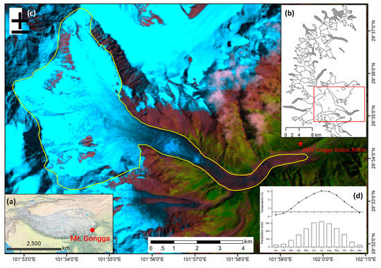
Figure 1.
The location of Mount Gongga (a) and the glacier distribution (b) on the Southeastern Tibetan Plateau. The main panel shows the Hailuogou glacier in a Landsat 5 TM image (combination of bands) acquired on 05 September 1994. The yellow line indicates the glacier extent of Hailuogou glacier in 1994, while the red star represents Mount Gongga Station (c), where the meteorological observations (d) have been recorded since 1987.
3. Materials and Methods
3.1. Satellite Images
Both Landsat 5 TM data and Landsat 8 TIRS data were obtained from the USGS website (https://glovis.usgs.gov/), with pixel resolutions of 120 m and 100 m for the infrared thermal bands (provided by the USGS/NASA at 30-m resolution); the advanced spaceborne thermal emission and reflection radiometer global digital elevation mode (ASTER GDEM) data were obtained in the same manner. A total of 99 clear-sky images spanning 28 complete hydrologic years (from 1990 to 2018) were used to retrieve GST (Table A1) in order to study its temporal variation during this period. Note that all images were selected seasonally (March–May for the spring, June–August for the summer, September–November for the autumn, and December–February for the winter) and based on cloud-free conditions over the glacier. One Sentinel-2 image (23 August 2018) was used to map the 2018 debris cover area, due to the Landsat 8 imagery in the summer of 2018 being relatively cloudy. At the same time, ground-based observation data (including near-surface air temperature, atmospheric water vapor, and groundwater vapor pressure data) were acquired from the Gongga Mountain Alpine Ecosystem Observation Station, Chinese Academy of Sciences (CAS) (elevation: 3000 m a.s.l.), and used for GST calculation.
3.2. GST Algorithms
In this paper, three algorithms were used to retrieve GST from Landsat thermal images. We follow the improved mono-window algorithm developed by Qin et al. [18] and compared the results with the radiative transfer equation (RTE) [39] and Jiménez-Muñoz and Sobrino’s single-channel method (JM_SC) [15]. In this section, we first present the general equation of the improved mono-window algorithm. More details follow regarding the calculation of at-sensor brightness temperature, determination of ground emissivity, estimation of effective mean atmospheric temperature, and estimation of atmospheric transmittance.
3.2.1. The Mono-Window Algorithm
This method is widely used in estimating land surface temperatures and is developed with data specific to only one infrared thermal band [18]. The equation is expressed as follows (i = 6 for Landsat 5 TM band 6, i = 10 for Landsat 8 TIRS band 10):
where Ts is the GST in degrees Celsius; Ti is the brightness temperature of Landsat 5 TM band 6 or Landsat 8 TIRS band 10; Ta is the effective mean atmospheric temperature; ai and bi are the constants used to approximate the derivative of the Planck radiance function for TM band 6 and TIRS band 10, given in Table 1; Ci and Di are the internal parameters for the algorithm, given as follows:
where εi is the ground emissivity and τi is atmospheric transmittance of Landsat 5 TM band 6 or Landsat 8 TIRS band 10. Three significant parameters (Ta, εi and τi) will be presented in the following sections.

Table 1.
Determination of the constants ai and bi for the different sensor types.
3.2.2. Calculation of the At-Sensor Brightness Temperature
The brightness temperature Ti plays an important role in the process of GST retrieval from Landsat infrared thermal band data via the mono-window algorithm (Equation (1)). Firstly, the digital numbers (DNs) will be transformed into thermal radiance, and then the DN value can be converted into the brightness temperature. Considering the differences between Landsat 5 and Landsat 8, the DN values for Landsat 5 TM band 6 and Landsat 8 TIRS band 10 can be converted into thermal radiance by Equation (4a) [40] and Equation (4b), respectively.
where L6 is the at-sensor thermal spectral radiance (m W cm−2 sr−1μm−1); Lmin6 and Lmax6 are the minimum and maximum detected spectral radiance, respectively; Qdn is the grey level for the analyzed pixel of the TM image; and Qmax is the maximum DN value. The values are given in Table 2.
where the L10 is the at-sensor thermal spectral radiance (W m−2 sr−1 μm−1) of TIRS band 10; Qdn is the grey level for the analyzed pixel of the TIRS image; M10 is the band-specific multiplicative rescaling factor for band 10; and A10 is the band-specific additive rescaling factor for band 10. The values of M10 and A10 can be acquired from the metadata file of Landsat 8 image, the values for which are presented in Table 3.
Table 2.
Parameters for computing at-sensor brightness temperatures from Landsat 5 TM band 6 data.
Table 3.
Parameters for computing at-sensor brightness temperature from Landsat 8 TIRS band 10 data.
With the computation of the thermal spectral radiance Li, the at-sensor brightness temperature can be calculated by using the approximation of the Planck radiance function, which is expressed as follows:
where Ti is the at-sensor brightness temperature (K); and K1 and K2 are the band-specific thermal conversion constants. For Landsat 5 TM band 6 data, K1 = 60.776 m W cm−2 sr−1μm−1 and K2 = 1260.56 K, respectively (Table 2). For Landsat 8 TIRS band 10 data, K1 = 774.89 W m−2 sr−1μm−1 and K2 = 1321.08 K, respectively (Table 3), which can also be acquired from the metadata file of the Landsat 8 image.
3.2.3. Determination of Ground Emissivity
Emissivity is related to the temperature, wavelength, surface roughness, observation angle, and composition of the surface, and is a key parameter for the surface temperature estimation. Several methods have been explored to simulate the land surface emissivity [41,42]. Owing to the fact that the NDVI(Normalized Difference Vegetation Index)-based emissivity method (NBEM) is inapplicable to this paper, we aim to calculate the GST by applying the semi-empirical model for the angular-dependent emissivity spectra of snow and ice in the 8–14 μm atmospheric window [43]. Hori et al. classified the transition from snow to ice categories: fine dendrite snow, medium granular snow, coarse-grained snow, sun crust, and bare ice. They assumed that the emissivity of snow and ice surfaces can be expressed by a linear combination of emissivities for the specular and blackbody surfaces, with weighting parameters characterizing the specularity of the bulk surface. The equations are expressed as follows and more details can be found in [27,43]:
where εsnow(λ, θ) is the angular-dependent emissivity of snow; λ is the wavelength; θ is the angle of exitance measured from the normal value; εbb(λ) is the emissivity of the isotropic blackbody (εbb(λ) = 1); fsp is the weighting parameter; εsp_app(λ, θ) is the apparent emissivity of the specular fraction; εsp(λ, θ) is the emissivity of an ideal smooth ice surface simulated with the Fresnel reflectance ρsp(λ, θ).
We used a band ratio approach to eliminate the impact of topography and enhance the discrimination between different snow grains. Based on three types of band ratio images ((Normalized Difference Snow Index, NDSI), Red/(Short-wave Infrared 1, SWIR1), (Near Infrared, NIR)/(Short-wave Infrared 1, SWIR1)), we utilized the K-mean unsupervised classification method together with previous field observations to classify the images into six categories: fine dendrite snow (fsp = 0.22), medium granular snow (fsp = 0.29), coarse-grained snow (fsp = 0.41), sun crust (fsp = 0.53), bare ice (fsp = 0.95), and glacier debris. In this paper, the emissivity of glacier debris has a fixed value of 0.941 [44].
3.2.4. Estimation of Effective Mean Atmospheric Temperature
Ground-based observations of effective atmospheric temperature (Ta) are hard to measure at the satellite pass time. Reviewing the previous literature, there are several methods that can be used to estimate the Ta. Sobrino et al. [45] developed a method that relates to the atmospheric temperature and water vapor content; this method is applicable for the places where the atmospheric profile data can be easily obtained at the satellite pass time. However, atmospheric profile data were lacking in this study. Here, we employ the method of Qin et al. [18], for which the standard atmospheric files and local meteorological data could be applied to estimate Ta. According to Qin et al. [18], the linear relations for approximation of Ta from the near-surface air temperature (To) are given in Table 4.
Table 4.
The linear relations for approximation of effective atmospheric temperature (Ta) from the near-surface air temperature (To) in the mid-latitude zone [18].
3.2.5. Estimation of Atmospheric Transmittance
Atmospheric transmittance is another essential parameter for GST retrieval. The atmospheric transmittance is influenced by the ozone, aerosol, wavelength, atmospheric chemicals, and atmospheric water vapor content (w), indicating the magnitude of thermal radiance absorption in the process of travelling to the sensor. It is commonly agreed that atmospheric water vapor content governs the atmospheric transmittance in the thermal channel. Two approaches could be used to estimate the atmospheric transmittance. The first one is to apply the atmospheric simulation program moderate-resolution atmospheric transmission (MODTRAN4) [46], while the second is to establish a function between atmospheric water vapor content and atmospheric transmittance. Here, we use the latter approach to simulate the atmospheric transmittance. Owing to the differences between Landsat 5 TM band 6 data and Landsat 8 TIRS band 10 data, the relation between atmospheric water vapor content and atmospheric transmittance can be found in Table 5.
Table 5.
The relation between atmospheric water vapor content and atmospheric transmittance for Landsat 5 TM band 6 data and Landsat 8 TIRS data. SEE, standard estimation error [17,18].
In the next step, the atmospheric water vapor content (w), which is unavailable directly, is estimated according to Yang et al. [47], using the equation:
where C0 and C1 are the empirical coefficients; W is the precipitable water. For the investigate area, C0 = 0.1274 and C1 = 0.6878, respectively. W can be estimated as follows:
where
With
and
in the equations above, e is the ground water vapor pressure (hPa); H is the elevation (km); Lat is the geographical latitude (°); a0 and a1 are the empirical coefficients calculated by Equations (11) and (12), respectively.
The near-surface air temperature and ground water vapor pressure recorded by the AWS can be obtained from the Gongga Mountain Alpine Ecosystem Observation Station, Chinese Academy of Sciences (CAS) (elevation: 3000 m a.s.l.).
3.3. Validation of GSTs
Previous studies suggested that the derived temperatures using the single-channel method exhibited a bias of 1 ℃, validated against in situ observation data [19]. By comparing three different methods for LST inversion from TIRS (the single-channel method, the split-window algorithm, and the radiative transfer equation), Yu et al. [39] found that temperatures derived from the radiative transfer equation were accurate, with a RMSE lower than 1 °C. Due to the limited samples of the ground observation data across the Hailuogou glacier, derived GSTs using the mono-window algorithm above were compared with two other single-channel algorithms (Jiménez-Muñoz and Sobrino’s single-channel method and the radiative transfer equation) [15,39] for the accuracy assessment. Here, we analyzed the accuracies across the entire study area over the images acquired in different seasons and from distinct sensor types (9 December 2017; 11 January 2013; 30 August 2006; 9 May 2000) (Table 6). The max bias was 1.3 °C, the average bias was 0.7 °C, and the average root mean square error (RMSE) was 0.7 °C when compared with the JM_SC. The max bias of the differences between derived temperatures and RTE was 3.7 °C, while the average bias and RMSE were 1.7 °C and 1.7 °C, respectively. It is noteworthy that the RTE is not accurate enough to retrieve land surface temperatures [48]. A scatter plot of the data (Figure 2) showed that the derived GSTs were in good agreement with the two other algorithms, indicating that the method mentioned in this paper can be adopted to study the spatial–temporal variations of the GSTs.
Table 6.
The results of the comparison between the remote-sensing-retrieved temperatures in this paper with two other single-channel algorithms. Jiménez-Muñoz et al.’s single-channel algorithm (JM_SC) is the method developed by Jiménez-Muñoz and Sobrino in 2003; RTE, radiative transfer equation.
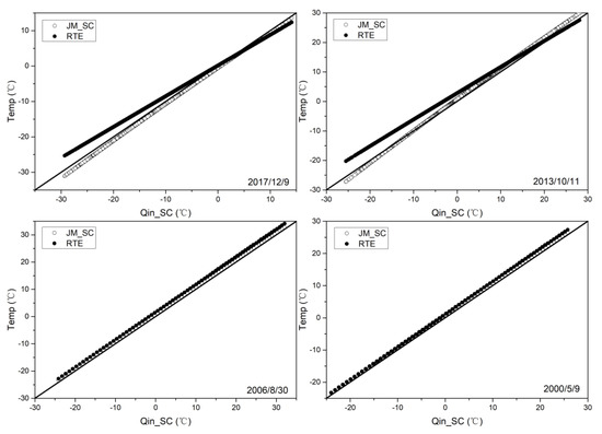
Figure 2.
Glacier surface temperatures (GSTs) calculated by the Qin et al.’s single-channel algorithm (Qin_SC) in this paper versus the JM_SC algorithm and radiative transfer equation (RTE).
4. Results
Here, we analyzed the spatial–temporal variations of Hailuogou glacier. For the spatial variation, we focused on the surface temperature gradient and the anomaly. Temporal variations (i.e., seasonal variation and interannual variation) were emphasized by certain metrics, such as the average surface temperature of the Hailuogou glacier, average temperatures in the debris-covered and debris-free areas, 0 ℃ isotherm elevation, and the extent of the glacier above 0 ℃.
4.1. Spatial Distribution Patterns of GSTs
For this purpose, we analyzed the GST spatial distribution patterns across Hailuogou glacier based on the image obtained by Landsat 8 on 10 November 2018. Looking at the entire glacier, the remote-sensing-retrieved temperature distribution shows that the surface temperature decreases with increasing elevation, while the mean temperature gradient is about −0.61 °C/100 m, which is slightly lower than the air temperature (−0.65 °C/100 m) (Figure 3a, Figure 4 and Figure 5). As can be seen in Figure 4, the lowest temperature is not at the top of glacier, while the highest temperature is located at the north side of glacier tongue, owing to the influences of the local topography (Figure 3b). Accordingly, surface temperatures across the accumulation area in the Hailuogou glacier show strong heterogeneity at the same elevation level (Figure 3a, Figure 4); part of the accumulation area would exceed 0 °C in summer due to the exposure of bedrock (Figure 5). In the ablation area, the surface temperatures on the north marginal area of the glacier tongue are higher than that on the south (Figure 3b,c). Notably, most of the pixels in the glacier tongue yield temperatures larger than 0 °C at the satellite passes, and elevations at which the surface temperature is 0 °C (we call this “0 °C isotherm elevation” in this paper) range from 3500 m a.s.l. to 5000 m a.s.l. (Figure 4 and Figure 5).
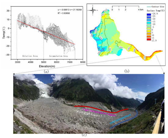
Figure 3.
Spatial patterns of surface temperatures on the Hailuogou glacier in clear daylight (10 November 2018): (a) the variation in the GSTs with elevation; (b) the distribution of GSTs across the Hailuogou glacier; (c) photograph of the glacier tongue.
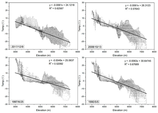
Figure 4.
Spatial patterns of surface temperatures on the Hailuogou glacier for the different seasons and sensor types (9 December 2017; 13 October 2008; 25 June 1997; 5 May 1990).
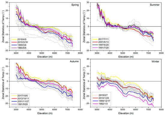
Figure 5.
Variations in the mean surface temperature zonal statistics for every 50 m within the elevation ranges on the Hailuogou glacier in different seasons; four profiles for each season are highlighted with colored lines.
4.2. Variations of GSTs between 1990–2018
A total of 99 cloud-free Landsat images over the glacier were utilized to study the temporal variations of surface temperatures on Hailuogou glacier. GSTs in summer are higher than in winter; the box-chart shows that GSTs change in a seasonal way and the average temperatures show a clear seasonal fluctuation (Figure 6 and Figure 7). A comparison between the station record air temperature and satellite-derived glacier surface temperature shows that the mean surface temperature on debris-covered areas is close to the station-recorded air temperature at 3000 m a.s.l. (Figure 7 and Figure 8a). As shown in Figure 8b, average temperatures in debris-covered and entire glacier areas both showed an increasing trend between 1990 and 2018, however the increase in the debris-covered area is more significant (Figure 8b). The 0 °C isothermal line elevations and extent of the glacier surface above the 0 °C isothermal line show some complexes in their long-term variations. The median value of the 0 °C isothermal line shows some variations between 4200 and 4800 m a.s.l. (Figure 9a), while the area of the glacier surface above the 0 °C isothermal line is more dynamic, but with an overall increasing trend for the median level since 1995 (Figure 9b). The increased extent of the glacier above 0 °C indicates that the ablation area of Hailuogou glacier has increased since 1995.
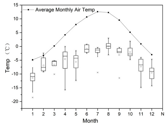
Figure 6.
The average monthly surface temperatures of Hailuogou glacier from 1990 to 2018. Box charts are the average surface temperature of Hailuogou glacier, while the black line with dots is the average monthly air temperature at the Mt. Gongga station (3000 m a.s.l.).
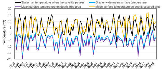
Figure 7.
Temporal variation of the station-recorded air temperatures and satellite-derived glacier surface temperatures.
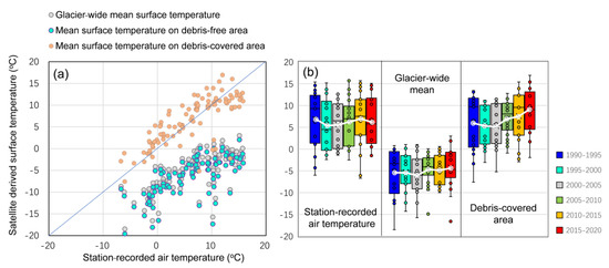
Figure 8.
(a) Comparison between the station-recorded air temperature and satellite-derived glacier surface temperature. (b) Statistics by box plots for the 5-year interval between 1990 and 2018 of station-recorded air temperatures and satellite-derived surface temperatures for the glacier-wide mean and debris-covered area. The dotted white lines indicate variation of means for each 5-year interval.
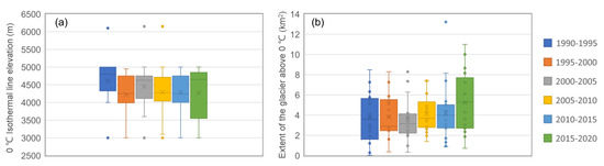
Figure 9.
Statistics by box plots for the 5-year interval between 1990 and 2018 of the 0 ℃ isothermal line elevation (a) and extent of the glacier surface above 0 ℃ (b).
5. Discussion
5.1. Errors in GST Remote Sensing
In this section, we first discussed the sources of errors in retrieving GST from Landsat thermal bands, although the remote-sensing-retrieved temperatures were in good agreement with the two other models. We believe that three major aspects would have important impacts on obtaining accurate GSTs, as follows: (1) The retrieved results would be hampered by cloud cover, which is frequently in the areas of mountain glaciers, resulting in a large number of remote sensing images being unavailable in this study. (2) It is possible that there is a mismatch in the locations of the glacier surfaces and satellite pixels. Additionally, one pixel represents the temperature of a quadrilateral (30 × 30 m), which is different from the measurements taken in the field. (3) Because natural surfaces are heterogeneous in terms of variations in emissivity, it is hard to determine the ground emissivity at the pixel scale; therefore, the derived emissivity should be taken in an effort to validate its accuracy.
5.2. Impacts of Glacier Debris Cover Expansion and Ice Surface Darkening on GSTs
The supraglacial debris plays a significant role in ice melting by controlling the surface temperature of the glacier. A debris layer of several centimeters would accelerate the ice melting owing to the lower albedo of debris cover, causing the surface to absorb more radiation compared to clean ice [34], while the debris layer would also insulate the glacier when the layer exceeded that thickness [49]. In most cases, the termini of debris-covered glaciers remain nearly stagnant, especially in Himalayan regions [50]. In the accumulation area of the Hailuogou glacier, the surface temperature shows great heterogeneity at the same elevation level because part of the area is covered by a debris layer, which is thinner than 3 cm (Figure 10). Both the debris cover in the lower part and the summer darkened ice surface in the upper part of the Hailuogou glacier have shown remarkable expansion since 1990 (Figure 11). Increasing accumulation of black carbon and dust on the glacier surface reduces the glacier albedo, increasing the net shortwave energy and resulting in higher surface temperatures.
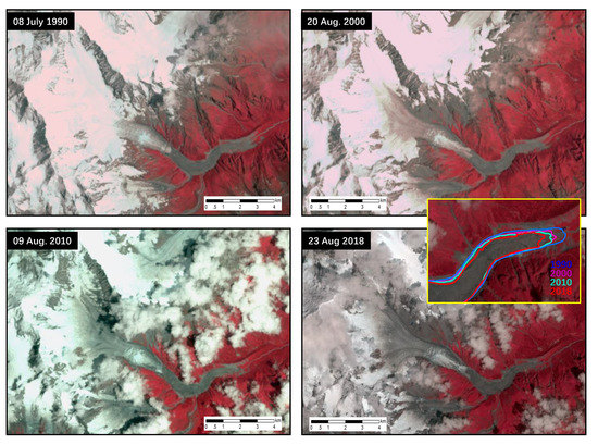
Figure 10.
Repeated summer satellite images between 1990 and 2018. Note the retreating debris-covered ice tongue of the Hailuogou glacier and increasing summer darkened area of the ice fall and the upper accumulation areas (showing the false color composites of TM for 1990, 2000, and 2010, and the false color composite of Sentinel-2 for 2018).
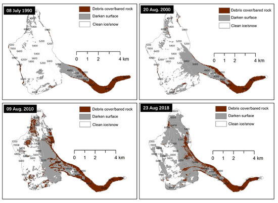
Figure 11.
Changing areas of debris cover, darkened ice surface, and clean ice and snow on the Hailuogou glacier in 1990, 2000, 2010, and 2018. The various areas of the glacier in 1990 are overlaid to highlight the retreating and shrinking ice tongue.
5.3. Effect of Topography on GSTs
The local topography impacts glacier surface temperatures by restricting illumination. There are three shading areas in the Hailuogou glacier—the first one is located near the top of the glacier, the second is at the glacier tongue, and the last is at the southern margin of the accumulation area (Figure 12). In the ablation area of the Hailuogou glacier, the topography dominates the spatial distribution. The glacier tongue surface is affected by thermal emissions from the surrounding topography. The distances between the surrounding cliffs and the glacier itself, however, can influence the magnitude of this effect [27]. Due to the reception of thermal reflection emitted from adjacent slopes, the northern margin of the glacier tongue shows a higher temperature than in the center or at the southern margin of the tongue. The southern margin of the glacier tongue is partly shaded by the north-facing topography (see the second shading area), thus exhibiting a lower surface temperature in most seasons. In the accumulation area of the Hailuogou glacier, the lowest temperature is not at the top of glacier because of the topographic shading (see the first shading area). The last shading area is not an anomaly, owing to the expansion of the exposed bedrock, which stops the occurrence of extremely low temperatures in the daytime (see the third shading area). The subsolar point changes periodically, being located in the northern hemisphere in summer and in the southern hemisphere in winter. The impact of topography in the summer is less than that in winter (Figure 4). Since the air temperature decreases with increasing elevation, the GSTs vary in a corresponding way with the elevation change. The steeper the slope (i.e., icefalls and ice cliffs), the higher the glacier surface temperature gradient. In general, the surface temperature on the south-facing slope is high, while that on the north-facing slope is low.
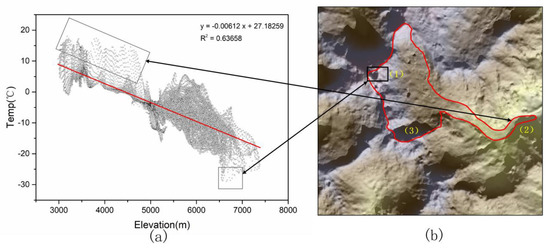
Figure 12.
The relationship between the anomaly and topographic shading: (a) the variation in the GSTs with elevation (10 November 2018); (b) the topographic shading of the Hailuogou glacier.
5.4. Climate as a Major Factor in the Temporal Variation of GSTs
In the context of global climate change, glaciers of the Tibetan Plateau have retreated over the past 50 years, and the retreat speed in the outer edge of this region is faster than that in the inner area [51,52]. Significant warming, especially in winter, is observed in the Tibetan Plateau based on in situ meteorological data from almost every weather station, whereby the annual mean air temperature increased by 0.16 °C per decade during the period 1955–1996 [53] and 0.35 °C per decade in the period 1961–2015 [54,55]. As shown in Figure 7 and Figure 8, the average surface temperature of the Hailuogou glacier varied consistently with air temperature, showing obviously seasonal fluctuations and an increasing trend (Figure 6 and Figure 8). As discussed above, dynamic climate change is a major factor in the temporal variation of glacier surface temperatures.
6. Conclusions
An attempt has been made in this paper to utilize the modified single-channel algorithm for GST retrieval from Landsat 8 TIRS data and Landsat 5 TM data. Three essential parameters (ground emissivity, effective mean atmospheric temperature, and atmospheric transmittance) are needed for GST retrieval with this method, and determinations of the three required parameters are presented with respective details in this study. GST has been used for the glacier mass balance and runoff modelling and debris thickness estimations, so it plays an important role in the evaluating glacier ablation rate and studying the glacier hydrology. In order to fill the gap in the study of long-term glacier surface temperature changes, the primary objective of this study, therefore, was to research the spatial–temporal variations of surface temperature across the Hailuogou glacier during 1990–2018. Although the remote-sensing-retrieved temperatures were not validated by the field measurements, this paper found that the method drives reasonable GSTs and can be applied to the Hailuogou glacier when compared to the two other algorithms.
The derived temperature distribution for the entire glacier shows that the surface temperature of the Hailuogou glacier generally decreases with increasing elevation, with a temperature gradient of −0.61 °C/1000 m. Owing to the presence of debris cover and exposed bedrock, temperatures across the accumulation area of the Hailuogou glacier show strong heterogeneity. In the ablation area, the topography is the main factor in the surface temperature distribution. For the time series of GSTs, both the glacier-wide mean surface temperature and 0 °C isotherm elevation show an increasing trend from 1990 to 2018, with rates of 0.054 °C a−1 and 12.415 m a−1, respectively. If these trends continue, the 0 °C isotherm elevation will rise to about 5100 m and a total area measuring 8 km2 will experience melting year-round in 50 years, which will result in the disappearance of the glacier landscape, a shortage of water resources, as well as frequent regional hazards. In general, the results from this study indicate that the Hailuogou glacier has become warmer and the ablation area has increased since 1990 because of the rising temperatures around the world.
Author Contributions
Conceptualization, Q.L.; methodology, H.L.; software, Y.Z.; validation, H.L. and Y.Z.; formal analysis, H.L. and X.L.; investigation, H.L.; data curation, H.L.; writing—original draft preparation, H.L.; writing—review and editing, Q.L. and X.L.; visualization, Y.Z.; project administration, Q.L.; funding acquisition, Q.L. All authors have read and agreed to the published version of the manuscript.
Funding
This work was funded by the National Natural Science Foundation of China (41871069; 41761144077) and Sichuan Science and Technology Program (2020JDJQ0002).
Acknowledgments
We would like to thank the Gongga Alpine Ecosystem Observation and Research Station, Chinese Academy of Sciences, for offering the meteorological data monitoring and field assistance. Satellite thermal images were from the U.S. Geological Survey (USGS); we thank the USGS for data support.
Conflicts of Interest
The authors declare no conflict of interest.
Appendix A
Details of the Landsat 5 TM data and Landsat 8 TIRS data that were used to derive GSTs in this paper are shown in Table A1.
Table A1.
Descriptions of the Landsat 5 TM data and Landsat 8 TIRS data.
Table A1.
Descriptions of the Landsat 5 TM data and Landsat 8 TIRS data.
| Date Acquired | Sensor Type | Path/ Row | Date Acquired | Sensor Type | Path/ Row | Date Acquired | Sensor Type | Path/ Row |
|---|---|---|---|---|---|---|---|---|
| 1990-05-05 | TM | 131/039 | 2000-08-20 | TM | 131/039 | 2009-11-26 | TM | 130/040 |
| 1990-07-08 | TM | 131/040 | 2000-11-24 | TM | 131/039 | 2010-01-20 | TM | 131/039 |
| 1990-12-24 | TM | 130/040 | 2000-12-26 | TM | 131/040 | 2010-03-18 | TM | 130/040 |
| 1991-04-15 | TM | 130/040 | 2001-05-03 | TM | 131/039 | 2010-08-09 | TM | 130/040 |
| 1991-07-20 | TM | 130/040 | 2001-06-13 | TM | 130/040 | 2010-10-12 | TM | 130/040 |
| 1991-09-29 | TM | 131/039 | 2001-11-27 | TM | 131/040 | 2011-01-07 | TM | 131/039 |
| 1992-01-03 | TM | 131/039 | 2002-01-14 | TM | 131/039 | 2011-04-29 | TM | 131/039 |
| 1992-05-03 | TM | 130/040 | 2002-10-13 | TM | 131/039 | 2011-08-12 | TM | 130/040 |
| 1992-08-07 | TM | 130/040 | 2003-02-18 | TM | 131/039 | 2011-10-06 | TM | 131/039 |
| 1992-11-18 | TM | 131/039 | 2003-04-16 | TM | 130/040 | 2013-04-18 | TIRS | 131/039 |
| 1993-01-30 | TM | 130/040 | 2003-07-21 | TM | 130/040 | 2013-07-07 | TIRS | 131/039 |
| 1993-04-27 | TM | 131/039 | 2003-09-23 | TM | 130/040 | 2013-10-11 | TIRS | 131/039 |
| 1993-07-09 | TM | 130/040 | 2004-02-14 | TM | 130/040 | 2013-12-30 | TIRS | 131/039 |
| 1993-12-07 | TM | 131/039 | 2004-04-25 | TM | 131/039 | 2014-04-14 | TIRS | 130/040 |
| 1994-04-30 | TM | 131/039 | 2004-06-12 | TM | 131/039 | 2014-07-26 | TIRS | 131/039 |
| 1994-06-26 | TM | 130/040 | 2004-11-28 | TM | 130/040 | 2014-11-08 | TIRS | 130/040 |
| 1994-09-05 | TM | 131/040 | 2005-01-06 | TM | 131/039 | 2015-02-03 | TIRS | 131/039 |
| 1994-12-26 | TM | 131/039 | 2005-04-05 | TM | 130/040 | 2015-05-10 | TIRS | 131/039 |
| 1995-04-10 | TM | 130/040 | 2005-09-19 | TM | 131/039 | 2015-07-06 | TIRS | 130/040 |
| 1995-08-07 | TM | 131/039 | 2006-02-26 | TM | 131/039 | 2015-10-26 | TIRS | 130/040 |
| 1995-10-10 | TM | 131/039 | 2006-05-17 | TM | 131/039 | 2016-01-05 | TIRS | 131/039 |
| 1996-02-15 | TM | 131/039 | 2006-08-30 | TM | 130/040 | 2016-03-18 | TIRS | 130/040 |
| 1996-03-02 | TM | 131/039 | 2006-11-18 | TM | 130/040 | 2016-08-16 | TIRS | 131/039 |
| 1996-10-12 | TM | 131/039 | 2006-12-27 | TM | 131/039 | 2016-11-04 | TIRS | 131/039 |
| 1997-06-25 | TM | 131/039 | 2007-04-18 | TM | 131/039 | 2017-01-07 | TIRS | 131/039 |
| 1998-04-09 | TM | 131/039 | 2007-06-14 | TM | 130/040 | 2017-03-28 | TIRS | 131/039 |
| 1998-07-30 | TM | 131/039 | 2007-09-18 | TM | 130/040 | 2017-07-11 | TIRS | 130/040 |
| 1998-09-16 | TM | 131/039 | 2008-04-04 | TM | 131/039 | 2017-10-06 | TIRS | 131/039 |
| 1999-01-22 | TM | 131/039 | 2008-07-18 | TM | 130/040 | 2017-12-09 | TIRS | 131/039 |
| 1999-03-04 | TM | 130/040 | 2008-10-13 | TM | 131/039 | 2018-04-09 | TIRS | 130/040 |
| 1999-11-06 | TM | 131/039 | 2009-02-18 | TM | 131/040 | 2018-08-31 | TIRS | 130/040 |
| 1999-12-17 | TM | 130/040 | 2009-04-16 | TM | 130/040 | 2018-11-10 | TIRS | 131/039 |
| 2000-05-09 | TM | 130/040 | 2009-06-03 | TM | 130/040 | 2019-02-07 | TIRS | 130/040 |
References
- Williamson, S.; Hik, D.; Gamon, J.; Kavanaugh, J.; Flowers, G. Estimating Temperature Fields from MODIS Land Surface Temperature and Air Temperature Observations in a Sub-Arctic Alpine Environment. Remote Sens. 2014, 6, 946–963. [Google Scholar] [CrossRef]
- Li, Z.L.; Tang, B.H.; Wu, H.; Ren, H.; Yan, G.; Wan, Z.; Trig, I.F.; Sobrino, J.A. Satellite-derived land surface temperature: Current status and perspectives. Remote Sens. Environ. 2013, 131, 14–37. [Google Scholar] [CrossRef]
- Kustas, W.; Anderson, M. Advances in thermal infrared remote sensing for land surface modeling. Agric. For. Meteorol. 2009, 149, 2071–2081. [Google Scholar] [CrossRef]
- Du, J.; He, Y.; Li, S.; Wang, S.; Niu, H.; Xin, H.; Pu, T. Mass balance and near-surface ice temperature structure of Baishui Glacier No.1 in Mt. Yulong. J. Geogr. Sci. 2013, 23, 668–678. [Google Scholar] [CrossRef]
- Xiao, H.; Weng, Q. The impact of land use and land cover changes on land surface temperature in a karst area of China. J. Environ. Manag. 2007, 85, 245–257. [Google Scholar] [CrossRef]
- Zhang, X.; Zhong, T.; Feng, X.; Wang, K. Estimation of the relationship between vegetation patches and urban land surface temperature with remote sensing. Int. J. Remote Sens. 2009, 30, 2105–2118. [Google Scholar] [CrossRef]
- Zaksek, K.; Oštir, K. Downscaling land surface temperature for urban heat island diurnal cycle analysis. Remote Sens. Environ. 2012, 117, 114–124. [Google Scholar] [CrossRef]
- Jansson, J.K.; Hofmockel, K.S. Soil microbiomes and climate change. Nat. Rev. Microbiol. 2019, 18, 35–46. [Google Scholar] [CrossRef] [PubMed]
- Albergel, C.; de Rosnay, P.; Gruhier, C.; Muñoz-Sabater, J.; Hasenauer, S.; Isaksen, L.; Kerr, Y.; Wagner, W. Evaluation of remotely sensed and modelled soil moisture products using global ground-based in situ observations. Remote Sens. Environ. 2012, 118, 215–226. [Google Scholar] [CrossRef]
- Nagornov, O.V.; Tyuflin, S.A.; Nikitaev, V.G.; Pronichev, A.N. Comparative analysis of the past glacier surface temperatures based on various probe-functions. J. Phys. Conf. Ser. 2017, 788, 012055. [Google Scholar] [CrossRef]
- Li, X.; Ding, Y.; Ye, B.; Han, T. Changes in physical features of Glacier No. 1 of the Tianshan Mountains in response to climate change. Chin. Sci. Bull. 2011, 56, 2820–2827. [Google Scholar] [CrossRef]
- He, Y.Q.; Li, Z.Q. Changes of the Hailuogou Glacier, Mt. Gongga, China, against the Background of Global Warming in the Last Several Decades. J. China Univ. Geosci. 2008, 19, 271–281. [Google Scholar]
- Mihalcea, C.; Brock, B.W.; Diolaiuti, G.; D’Agata, C.; Citterio, M.; Kirkbride, M.P.; Cutler, M.E.J.; Smiraglia, C. Using ASTER satellite and ground-based surface temperature measurements to derive supraglacial debris cover and thickness patterns on Miage Glacier (Mont Blanc Massif, Italy). Cold Reg. Sci. Technol. 2008, 52, 341–354. [Google Scholar] [CrossRef]
- Groos, A.R.; Mayer, C.; Smiraglia, C.; Diolaiuti, G.; Lambrecht, A. A First Attempt to Model Region-Wide Glacier Surface Mass Balances in the Karakoram: Findings and Future Challenges. Geogr. Fis. Din. Quat. 2017, 40, 137–159. [Google Scholar]
- Jiménez-Muñoz, J.C.; Sobrino, J.A. A generalized single-channel method for retrieving land surface temperature from remote sensing data. J. Geophys. Res. Atmos. 2003. [Google Scholar] [CrossRef]
- Wan, Z.M.; Dozier, J. A generalized split-window algorithm for retrieving land-surface temperature from space. IEEE Trans. Geosci. Remote Sens. 1996, 34, 892–905. [Google Scholar] [CrossRef]
- Wang, F.; Qin, Z.; Song, C.; Tu, L.; Karnieli, A.; Zhao, S. An Improved Mono-Window Algorithm for Land Surface Temperature Retrieval from Landsat 8 Thermal Infrared Sensor Data. Remote Sens. 2015, 7, 4268–4289. [Google Scholar] [CrossRef]
- Qin, Z.; Karnieli, A.; Berliner, P. A mono-window algorithm for retrieving land surface temperature from Landsat TM data and its application to the Israel-Egypt border region. Int. J. Remote Sens. 2010, 22, 3719–3746. [Google Scholar] [CrossRef]
- Cristóbal, J.; Jiménez-Muñoz, J.; Prakash, A.; Mattar, C.; Skoković, D.; Sobrino, J. An Improved Single-Channel Method to Retrieve Land Surface Temperature from the Landsat-8 Thermal Band. Remote Sens. 2018, 10, 431. [Google Scholar] [CrossRef]
- Sobrino, J.A.; Jiménez-Muñoz, J.C.; Paolini, L. Land surface temperature retrieval from LANDSAT TM 5. Remote Sens. Environ. 2004, 90, 434–440. [Google Scholar] [CrossRef]
- Wang, S.; He, L. Practical split-window algorithm for retrieving land surface temperature over agricultural areas from ASTER data. J. Appl. Remote Sens. 2014, 8, 083582. [Google Scholar] [CrossRef]
- Cahyono, A.B.; Saptarini, D.; Pribadi, C.B.; Armono, H.D. Estimation of Sea Surface Temperature (SST) Using Split Window Methods for Monitoring Industrial Activity in Coastal Area. Appl. Mech. Mater. 2017, 862, 90–95. [Google Scholar] [CrossRef]
- Anding, D.; Kauth, R. Estimation of sea surface temperature from space. Remote Sens. Environ. 1970, 1, 217–220. [Google Scholar] [CrossRef]
- Schneider, K.; Mauser, W. Processing and accuracy of Landsat Thematic Mapper data for lake surface temperature measurement. Int. J. Remote Sens. 2007, 17, 2027–2041. [Google Scholar] [CrossRef]
- Stroeve, J.; Steffen, K. Variability of AVHRR-derived clear-sky surface temperature over the Greenland ice sheet. J. Appl. Meteorol. 1998, 37, 23–31. [Google Scholar] [CrossRef]
- Haq, M.A.; Jain, K.; Menon, K.P.R. Surface Temperature Estimation of Gangotri Glacier Using Thermal Remote Sensing. Int. Arch. Photogramm. 2012, 39, 115–119. [Google Scholar]
- Wu, Y.; Wang, N.; He, J.; Jiang, X. Estimating mountain glacier surface temperatures from Landsat-ETM + thermal infrared data: A case study of Qiyi glacier, China. Remote Sens. Environ. 2015, 163, 286–295. [Google Scholar] [CrossRef]
- Kraaijenbrink, P.D.A.; Shea, J.M.; Litt, M.; Steiner, J.F.; Treichler, D.; Koch, I.; Immerzeel, W.W. Mapping Surface Temperature on a Debris-Covered Glacier With an Unmanned Aerial Vehicle. Front. Earth Sci. 2018, 6, 64. [Google Scholar] [CrossRef]
- Aubry-Wake, C.; Baraer, M.; McKenzie, J.M.; Mark, B.G.; Wigmore, O.; Hellström, R.Å.; Lautz, L.; Somers, L. Measuring glacier surface temperatures with ground-based thermal infrared imaging. Geophys. Res. Lett. 2015, 42, 8489–8497. [Google Scholar] [CrossRef]
- He, M.H. Forty Year’s Study of Glacier Temperature Distribution in China: Review and Suggestions. J. Glaciolgy Geocryol. 1999, 21, 310–316. [Google Scholar]
- Zhang, Y.; Fujita, K.; Liu, S.Y.; Liu, Q.; Nuimura, T. Distribution of debris thickness and its effect on ice melt at Hailuogou glacier, southeastern Tibetan Plateau, using in situ surveys and ASTER imagery. J. Glaciol. 2011, 57, 1147–1157. [Google Scholar] [CrossRef]
- Jian-Chen, P.U.; Su, Z.; Yao, T.D.; Xie, Z.C. Mass Balance on Xiao Dongkemadi Glacier and Hailuogou Glacier. J. Glaciolgy Geocryol. 1998, 20, 408–412. [Google Scholar]
- Mlg, N.; Bolch, T.; Rastner, P.; Strozzi, T.; Paul, F. A consistent glacier inventory for the Karakoram and Pamir regions derived from Landsat data: Distribution of debris cover and mapping challenges. Earth Syst. Sci. Data Discuss. 2018, 10, 1807–1827. [Google Scholar] [CrossRef]
- Zhang, Y.; Hirabayashi, Y.; Fujita, K.; Liu, S.Y.; Liu, Q. Heterogeneity in supraglacial debris thickness and its role in glacier mass changes of the Mount Gongga. Sci. China Earth Sci. 2016, 59, 170–184. [Google Scholar] [CrossRef]
- Sun, H.Y.; Wu, Y.H.; Zhou, J.; Bing, H.J. Variations of bacterial and fungal communities along a primary successional chronosequence in the Hailuogou glacier retreat area (Gongga Mountain, SW China). J. Mt. Sci. 2016, 13, 1621–1631. [Google Scholar] [CrossRef]
- Liu, Q.; Liu, S.Y.; Zhang, Y.; Zhang, Y.S. Surface Ablation Teatures and Recent Variation of the Lower Ablation Area of the Hailuogou glacier, Mt. Gongga. J. Glaciol. Geocryol. 2011, 33, 227–236. [Google Scholar]
- Zhang, Y.; Fujita, K.; Liu, S.Y.; Liu, Q.; Wang, X. Multi-decadal ice-velocity and elevation changes of a monsoonal maritime glacier: Hailuogou glacier, China. J. Glaciol. 2010, 56, 65–74. [Google Scholar] [CrossRef]
- Lu, Q.; Liu, S.Y.; Zhang, Y.; Xin, W.; Zhang, Y.; Guo, W.; Xu, J. Recent Shrinkage and Hydrological Response of Hailuogou Glacier, a Monsoon Temperate Glacier on the East Slope of Mount Gongga, China. J. Glaciol. 2010, 56, 215–224. [Google Scholar] [CrossRef]
- Yu, X.; Guo, X.; Wu, Z. Land Surface Temperature Retrieval from Landsat 8 TIRS—Comparison between Radiative Transfer Equation-Based Method, Split Window Algorithm and Single Channel Method. Remote Sens. 2014, 6, 9829–9852. [Google Scholar] [CrossRef]
- Barsi, J.A.; Hook, S.J.; Schott, J.R.; Raqueno, N.G.; Markham, B.L. Landsat-5 Thematic Mapper Thermal Band Calibration Update. IEEE Geosci.Remote Sens. Lett. 2007, 4, 552–555. [Google Scholar] [CrossRef]
- Sobrino, J.A.; Jimenez-Muoz, J.C.; Sòria, G.; Romaguera, M.; Guanter, L.; Moreno, J.; Plaza, A.; Martínez, P. Land surface emissivity retrieval from different VNIR and TIR sensors. IEEE Trans. Geosci. Remote Sens. 2008, 46, 316–327. [Google Scholar] [CrossRef]
- Li, Z.L.; Wu, H.; Wang, N.; Qiu, S.; Sobrino, J.A.; Wan, Z.; Tang, B.H.; Yan, G. Land surface emissivity retrieval from satellite data. Int. J. Remote Sens. 2013, 34, 3084–3127. [Google Scholar] [CrossRef]
- Hori, M.; Aoki, T.; Tanikawa, T. Modeling angular-dependent spectral emissivity of snow and ice in the thermal infrared atmospheric window. Appl. Opt. 2013, 52, 7243–7255. [Google Scholar] [CrossRef]
- Rees, W.G. Infrared emissivities of Arctic land cover types. Int. J. Remote Sens. 2007, 14, 1013–1017. [Google Scholar] [CrossRef]
- Sobrino, J.; Coll, C.; Caselles, V. Atmospheric correction for land surface temperature using NOAA-11 AVHRR channels 4 and 5. Remote Sens. Environ. 1991, 38, 19–34. [Google Scholar] [CrossRef]
- Berk, A.; Anderson, G.P.; Bernstein, L.S.; Acharya, P.K.; Dothe, H.; Matthew, M.W.; Adler-Golden, S.M.; Chetwynd, J.H.; Richtsmeier, S.C.; Pukall, B. MODTRAN4 Radiative Transfer Modeling for Atmospheric Correction. In Proceedings of the Optical Spectroscopic Techniques and Instrumentation for Atmospheric and Space Research III, Denver, CO, USA, 19–21 July 1999. [Google Scholar]
- Yang, J.M.; Qiu, J.H. A Method for Estimating Precipitable Water and Effective Wate Wapor Content from Ground Humidity Parameters. Chin. J. Atmos. Sci. 2002, 26, 9–22. [Google Scholar]
- Huang, M.F.; Xing, X.F.; Wang, P.J.; Wang, C.Z. Comparison between three different methods of retrieving surface temperature from Landsat TM thermal infrared band. Arid Land Geogr. 2006, 19, 132–137. [Google Scholar]
- Rounce, D.R.; Mckinney, D.C. Debris thickness of glaciers in the Everest Area (Nepal Himalaya) derived from satellite imagery using a nonlinear energy balance model. Cryosphere 2014, 8, 1317–1329. [Google Scholar] [CrossRef]
- Jiang, S.; Nie, Y.; Liu, Q.; Wang, J.; Liu, L.; Hassan, J.; Liu, X.; Xu, X. Glacier Change, Supraglacial Debris Expansion and Glacial Lake Evolution in the Gyirong River Basin, Central Himalayas, between 1988 and 2015. Remote Sens. 2018, 10, 986. [Google Scholar] [CrossRef]
- Li, Z.G. Glacier and Lake Changes across the Tibetan Plateau during the Past 50 Years of Climate Change. J. Resour. Ecol. 2014, 5, 123–131. [Google Scholar]
- Sun, Y.; Jiang, L.; Lin, L.; Sun, Q.; Hsu, H. Mapping Glacier Elevations and Their Changes in the Western Qilian Mountains, Northern Tibetan Plateau, by Bistatic InSAR. IEEE J. Sel. Top. Appl. Earth Obs. Remote Sens. 2017, 11, 68–78. [Google Scholar] [CrossRef]
- Liu, X.; Chen, B. Climatic warming in the Tibetan Plateau during recent decades. Int. J. Climatol. 2020, 20, 1729–1742. [Google Scholar] [CrossRef]
- Xu, Y.; Knudby, A.; Ho, H.C.; Shen, Y.; Liu, Y. Warming over the Tibetan Plateau in the last 55 years based on area-weighted average temperature. Reg. Environ. Chang. 2017, 17, 2339–2347. [Google Scholar] [CrossRef]
- Cai, D.; You, Q.; Fraedrich, K.; Guan, Y. Spatiotemporal Temperature Variability over the Tibetan Plateau: Altitudinal Dependence Associated with the Global Warming Hiatus. J. Clim. 2017, 30, 969–984. [Google Scholar] [CrossRef]


© 2020 by the authors. Licensee MDPI, Basel, Switzerland. This article is an open access article distributed under the terms and conditions of the Creative Commons Attribution (CC BY) license (http://creativecommons.org/licenses/by/4.0/).