Abstract
This study aimed to understand which vegetation indices (VIs) are an ideal proxy for describing phenology and interannual variability of Gross Primary Productivity (GPP) in short-rotation coppice (SRC) plantations. Canopy structure- and chlorophyll-sensitive VIs derived from Sentinel-2 images were used to estimate the start and end of the growing season (SOS and EOS, respectively) during the period 2016–2018, for an SRC poplar (Populus spp.) plantation in Lochristi (Belgium). Three different filtering methods (Savitzky–Golay (SavGol), polynomial (Polyfit) and Harmonic Analysis of Time Series (HANTS)) and five SOS- and EOS threshold methods (first derivative function, 10% and 20% percentages and 10% and 20% percentiles) were applied to identify the optimal methods for the determination of phenophases. Our results showed that the MEdium Resolution Imaging Spectrometer (MERIS) Terrestrial Chlorophyll Index (MTCI) had the best fit with GPP phenology, as derived from eddy covariance measurements, in identifying SOS- and EOS-dates. For SOS, the performance was only slightly better than for several other indices, whereas for EOS, MTCI performed markedly better. The relationship between SOS/EOS derived from GPP and VIs varied interannually. MTCI described best the seasonal pattern of the SRC plantation’s GPP (R2 = 0.52 when combining all three years). However, during the extreme dry year 2018, the Chlorophyll Red Edge Index performed slightly better in reproducing growing season GPP variability than MTCI (R2 = 0.59; R2 = 0.49, respectively). Regarding smoothing functions, Polyfit and HANTS methods showed the best (and very similar) performances. We further found that defining SOS as the date at which the 10% or 20% percentile occurred, yielded the best agreement between the VIs and the GPP; while for EOS the dates of the 10% percentile threshold came out as the best.
1. Introduction
Short-rotation coppice (SRC) plantations provide multiple economic and ecological benefits [1]. They are ideal for producing biomass for energy [2] and can, therefore, substitute for fossil fuels to reduce anthropogenic CO2 emissions [3]. They enrich farm-scale biodiversity [4], increase soil organic carbon stock [5,6], improve groundwater quality [7] and help in preventing pests and diseases. Over 16% of woodlands in Europe were managed as coppice in 2000, covering a global area of about 23 million ha [8]. In the last 20 years, SRC plantations increased globally to cover an area of 31.8 million ha in 2016 [9]. Poplars (Populus spp.) are widely used as bioenergy plantations and for wood production in the Northern Hemisphere representing 99% (31.4 million ha) of SRC area worldwide.
Even though the important role of SRC plantations in bioenergy productions and carbon sequestration is well recognized by the scientific community [10,11], data on SRC productivity (e.g., Gross Primary Productivity (GPP)) and phenology are scarce and limited to small experimental areas.
The ecosystem phenology, also defined as carbon flux phenology, describes the seasonality of the gross photosynthesis (i.e., GPP) of an ecosystem. The starting day of the photosynthetic season (SOS) occurs when an ecosystem turns from a carbon source into a carbon sink in spring. Contrary, the end of the season (EOS) identifies the decrease of photosynthetic activity at the beginning of senescence. A shift in the SOS and EOS of a growing season regulates annual GPP [12,13]. A longer growing season increases the annual productivity of deciduous forests [14,15]. The timing of bud bursts and sets depend on local environmental conditions. The plant growth strategy of deciduous trees in temperate regions exploits maximally optimal spring growth conditions [16]. SRC plantations allocate carbon to different tree components at the beginning of the growing season [17] as reported also for beech in Campioli et al. (2011). The photosynthetic activity shows a substantial decline by early mid-September in temperate deciduous species [18]. Contrary, high carbon uptake rates were observed until the end of September for SRC plantations [17,19] and poplar [20]. Furthermore, for agroecosystems such as crops and SRC plantations, management practices also play an important role in determining the annual production. However, few studies focused on the understanding of the effect of coppicing on SRC phenology [21,22]. A clear understanding of how phenology affects the productivity of SRC plantation can effectively support farmers in optimally managing their fields to obtain the most profit from crop production. In addition, it is necessary to improve the model parameterization of global productivity models.
In situ observations provide a robust measurement of plant development and phenology [22], but they can be laborious and expensive when a lot of sites need to be sampled. The eddy covariance (EC) method [23] is suitable for monitoring ecosystem productivity, aspects of phenology and their changes related to abiotic stresses (e.g., drought, management) [24,25]. However, GPP data derived from the EC method are representative of only a small area, roughly speaking 10 to 30 times the measurement height on average, around and mostly upwind of the flux tower [26] and the technique has rarely been applied at SRC plantations. Both EC and in situ observations thus have limitations when data sampling is required at large spatial scales.
Large-scale and continuous observations taken by satellite sensors make remote sensing approaches attractive alternatives for phenology assessment [27,28]. Spectral vegetation indices (VIs) can be used to derive many biophysical and biochemical vegetation parameters (e.g., chlorophyll content, Leaf Area Index (LAI)) and GPP [29,30,31,32,33,34,35]. The Normalized Difference Vegetation Index (NDVI) [36] and the Enhanced Vegetation Index (EVI) [37] (referring to Table 1) are the most commonly used VIs for monitoring canopy greenness, development and phenology [38]. Due to its long time-series, NDVI has been widely used as a proxy for GPP [39,40] and the analysis of ecosystem phenology [28,41,42,43,44]. Research, however, has shown that both NDVI and EVI can fail to predict canopy phenology and productivity when LAI is high and in specific periods of the year, especially when canopy greenness and physiology are decoupled, e.g., during drought [45,46] and senescence [47,48]. Chlorophyll-sensitive VIs appear to be better suited for monitoring the phenology of plants and crops [49], because they are indirect proxies of canopy biochemistry. For example, green NDVI (gNDVI) considers the green band, which is more closely related to chlorophyll (see Table 1) than the red band [50], which is used in NDVI. gNDVI is better correlated with LAI than are NDVI and EVI and improves the modeling of LAI [51]. The Chlorophyll Index (ChlRedEdge) and the MERIS Terrestrial Chlorophyll Index (MTCI) also correlate with chlorophyll content [52,53,54] and should, in theory, be good proxies for phenology and GPP seasonality of crops. Pigment Specific Simple Ratio (PSSR) was reported to have a strong relationship with chlorophyll content [29,55]. Modified Chlorophyll Absorption Ratio (MCARI) is an alternative index that provides a measure of chlorophyll concentration [56,57] but is also sensitive to nonphotosynthetic components of the canopy, especially at low chlorophyll concentrations [58]. The Structure Insensitive Pigment Index (SIPI) is associated with the ratio of carotenoids to chlorophylls and allows mitigating the effects of foliar structural properties on reflectance, because it considers the NIR band [59,60,61]. Thus, a wide suite of RS-based indices can provide information on SRC phenology and possibly productivity. However, to date, the phenology and GPP seasonality of SRC plantations have not yet been widely studied via VIs, probably due to the poor spatial (1 km or larger) and spectral resolution (red and NIR mainly) of satellite sensors (e.g., MODIS/Terra or MODIS/Aqua; SPOT/VGT, NOAA/AVHRR; Landsat) [22].

Table 1.
Vegetation indices (VIs) derived from Sentinel-2. Abbreviations correspond with center wavelengths, in nm: B02 = reflectance at 490 nm; B03 = reflectance at 560 nm; B04 = reflectance at 665 nm; B05 = reflectance at 705 nm; B06 = reflectance at 740 nm; B08 = reflectance at 842 nm. B02, B04 and B08 have a 10 m spatial resolution, while B05 and B06 have a 20 m resolution.
A wide range of time-series smoothing methods and extracting phenological metrics (SOS, EOS) to reconstruct the seasonal patterns of noisy VI time-series have been proposed [27,62,63]. However, there is no single method that always performs better than another for smoothing VI time-series [64]. Large discrepancies in the detection of SOS and EOS have been found by comparing different retrieval methods [65,66,67] and no conclusive evidence favors one method over another. Therefore, combining multiple methods should provide better estimates of phenological metrics.
The recent advent of high-resolution Sentinel-2 satellite imagery, with a spatial resolution of 10, 20 and 60 m offers a new perspective in monitoring ecosystem phenology. This satellite has two main advantages over other high-resolution satellites such as Landsat. The five-day temporal resolution is an advantage for monitoring plants, and the 10 m spatial resolution is more suitable for ecological, agricultural and phenological studies [71,72]. Another interesting feature of Sentinel-2 is the availability of additional red-edge bands, which are available from other few space-borne sensors [73]. These red-edge regions play an important role in estimating the biochemical and biophysical traits of plants [74].
In this study we explored for the first time the use of eight canopy structure- and chlorophyll-sensitive VIs, derived from Sentinel-2, for describing the phenology and seasonal variability of GPP, derived from EC, of an SRC poplar plantation in Belgium. The objectives of this study were three-fold: (i) to understand which VI could be an ideal proxy of GPP phenology of SRC plantations, (ii) to identify optimal filtering and threshold methods for describing phenological metrics and (iii) to analyze the performance of each VI in capturing the seasonal variability of GPP.
2. Materials and Methods
2.1. Site Description
The study site was a poplar based SRC plantation of 8 ha located in Lochristi, Belgium (51°06′44″N, 3°51′02″E; 6 m a.s.l.; Figure 1, red polygon). The plantation was established in April 2010 in the framework of the POPFULL project (https://webhosting.uantwerpen.be/popfull/index.php?page=project&lang=en). A complete description of the experimental site and plant material has been previously published [75,76]. In brief, the plantation consists of 12 poplar (Populus) genotypes planted in monoclonal blocks at a density of 8000 trees ha-1. Poplars are planted in a double-row planting scheme with an alternating interrow spacing of 0.75 m and 1.50 m and an intrarow distance between each tree of 1.10 m. Details of plant development and phenological metrics have been provided by Vanbeveren et al. (2016). The plantation was harvested for the third time in February 2017, after earlier coppices in 2014 and 2012. We focused on the years 2016 (the third and last year of the third rotation), 2017 (the first year of the fourth rotation) and 2018 (the second year of the fourth rotation).
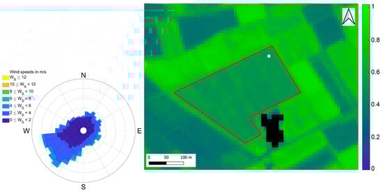
Figure 1.
Normalized Difference Vegetation Index (NDVI) Sentinel-2 image of the short-rotation coppice (SRC) plantation in Lochristi acquired on 7 July 2016, at 10 m resolution. The red polygon is the area of the plantation. The same area was extracted for calculating VIs. The white dot indicates the location of the flux tower. The black pixels represent the outbuildings. On the left, the wind rose for 2016 representing the wind direction distribution for wind speed classes.
2.2. Measurement of CO2 Fluxes and Estimation of GPP
The study site was equipped with an EC system to monitor continuously the CO2 net flux between the surface and atmosphere, also called Net Ecosystem Exchange (NEE). The system was composed of a Gill-HS50 sonic anemometer (Gill Instruments Ltd., Lymington, UK) for measuring 3D wind speed components and sonic temperature and of an LI-7200 enclosed-path infrared gas analyzer (LI-COR Inc., Lincoln, NB, USA) for measuring CO2 and H2O concentrations. Both instruments collected measurements at a frequency of 10 Hz. CO2 and H2O concentrations and fluxes of latent and sensible heat were estimated every 30 min using a standard scheme for processing the raw EC data. Briefly, flux data collected during conditions of well-developed turbulence and a good level of stationarity with sustained mechanical turbulence were used for the analysis according to CARBOEUROPE methodology [77]. The location of the tower was on the north-east edge of the plantation (Figure 1). To maximize the representativeness of flux measurements collected at the EC tower, data with wind direction between 50° and 250° were retained for the analysis [78] (Figure 1, wind rose). A more detailed description of the experimental setup, the calculations applied to the raw EC data and the criteria used to filter the entire data set have been previously reported by [11,19]. Complete details of the EC methodology, processing schemes and corrections are also available [77,79].
Other meteorological variables were continuously measured and averaged every 30 min at the site: global solar radiation (Rg) was measured using a CG3 pyranometer (Kipp and Zonen B.V., Delft, The Netherlands), air temperature and relative humidity were measured using an HMP155A thermohygrometer (Vaisala Oyj, Vantaa, Finland) and soil water content at a depth of 20 cm was measured using CS650 time-domain reflectometric probes (Campbell Scientific Inc., Logan, UT, USA).
GPP was estimated from the measured NEE by partitioning it into its two main components: GPP and ecosystem respiration , following the well-established relationship , where Reco is modeled from NEE night-time data as a function of measured air temperature [80,81]. The full time-series of the three variables have been obtained by filling unavoidable gaps in the measured NEE time-series, using the methodology for gap-filling and partitioning described by Reichstein et al. (2005). Numerical results were obtained using the REddyProc online tool provided by the Max Planck Institute (https://www.bgc-jena.mpg.de/bgi/index.php/Services/REddyProcWeb). We averaged half-hourly GPP values between 10:00 and 14:00 solar local time to allow for direct comparison with the Sentinel-2 satellite data acquisition. These values are indicated hereafter as GPP, while daily sums of GPP are indicated as daily GPP.
2.3. VIs
In this study, we used the European Space Agency Sentinel-2 TOC (Top Of Canopy) satellite images provided by the Terrascope platform (https://www.terrascope.be). This platform provides access to a data set of processed Sentinel-2 images covering Belgium. Sentinel-2 carries a Multispectral Instrument (MSI) that samples 13 spectral bands in the visible and NIR regions at 10, 20 or 60 m resolutions depending on the spectral band (https://sentinel.esa.int/web/sentinel/home). The whole time-series of Sentinel-2 data from 1 January 2016 to 31 December 2018 were used in this study. The long cloudy and rainy periods in this area, mainly in 2016, affected the quality of satellite time-series. After the quality check, 15 images were retained for 2016, 24 for 2017 and 23 in 2018. From the Sentinel-2 time-series an area of 8 ha corresponding to the area of the plantation was extracted first from the Sentinel-2 time-series for each available day (Figure 1, red polygon). A total of about 800 pixels were extracted for the bands at a resolution of 10 m and 200 pixels were extracted for the bands at a resolution of 20 m (see Table 1 for more details). Secondly, using the cloud mask available for this data set, each pixel was quality checked and only cloud-free days were selected for further analysis [82]. Third, the values of the retained good pixels in the extracted area were averaged for each band, and VIs were derived. Eight VIs were calculated over all available images of the time-series: the Normalized Difference Vegetation Index (NDVI), the Enhanced Vegetation Index (EVI), the MERIS Terrestrial Chlorophyll Index (MTCI), the Chlorophyll Red Edge Index (ChlRedEdge), the Modified Chlorophyll Absorption Reflectance Index (MCARI), the Pigment Specific Simple Ratio (PSSR), the Structure Insensitive Pigment Index (SIPI) and the green NDVI (gNDVI). The vegetation indices were calculated with Sentinel-2 bands B02, B03, B04, B05, B06 and B08, using the formulas reported in Table 1. The Sentinel-2 bands have the following band centers; B02: 490 nm; B03: reflectance at 560 nm; B04: reflectance at 665 nm; B05: reflectance at 705 nm; B06: reflectance at 740 nm; B08: reflectance at 842 nm. B02, B04 and B08 have a 10 m spatial resolution, while B05 and B06 have a 20 m resolution.
The NDVI and the EVI are the most known and used spectral indices for monitoring canopy greenness, development and phenology [38]. However, both the NDVI and the EVI have shown to fail in predicting the canopy phenology and productivity in specific periods of the year, especially when canopy greenness and physiology are decoupled, i.e., during drought [45] and senescence [47]. For that reason, in this study, we also considered VIs that correlate with canopy pigments and, therefore, are indirect proxies of canopy biochemistry. In particular, the gNDVI is more sensitive to chlorophyll. The ChlRedEdge and the MTCI indirectly correlate with chlorophyll content [52,53,54]. The PSSR was reported to have a strong relationship with chlorophyll content [29,55] while MCARI correlates to chlorophyll concentration [56,57]; the Structure Insensitive Pigment Index (SIPI) is sensitive to the ratio of carotenoids to chlorophyll [61].
2.4. Extracting Phenology Indicators from GPP and VIs
Dates for SOS and EOS were derived from time-series for both GPP and VIs. Three smoothing methods were applied to the raw time-series data to reduce noise and fill gaps in the occasionally poor coverage: Savitzky–Golay (SavGol), Harmonic Analysis of Time Series (HANTS) and polynomial (Polyfit).
All data of the fitted time-series before the period with the highest GPP (April−June) were selected for identifying SOS while the remaining data were selected for identifying EOS. Five different threshold methods were applied to both data sets to identify SOS and EOS, respectively.
2.4.1. Filtering Methods
The study area was characterized by long rainy and cloudy periods, mainly in the year 2016. For that reason, we selected three smoothing functions, whose in regions with a long period of cloudiness and a high atmospheric variability are well documented [28,83,84]: Savitzky–Golay (SavGol), Harmonic Analysis of Time Series (HANTS) and polynomial (Polyfit).
The SavGol filter is a robust method to reduce efficiently the cloud and snow contamination in the time-series [84,85]. It is a low-pass filter that smooths the time-series applying a polynomial regression function to x data points in a moving window [86]:
For all points within the time window, a polynomial function of n degree was solved. In this study, the window size and the degree of the polynomial fitting function have been defined for each time-series data (i.e., VIs and GPP). In every window, a new polynomial was fitted. Subsequently, the window moved to the next part of the input dataset, a new local polynomial function was fitted to the original data in this window, and a new data point was calculated. This process was repeated for all remaining time windows. The parameters used to smooth both VIs and GPP time-series are reported in Table 2. We obtained these parameters using Python 3.6 package scipy.signal and the function SavGol filter (https://scipy.org/).
Table 2.
Parameters used for Savitzky–Golay (SavGol) and polynomial (Polyfit) methods for filtering time-series of Gross Primary Productivity (GPP) and VIs (see VIs definitions in Table 1) per each year. n—degree of polynomial function; x—data points in the moving window used for the SavGol method.
HANTS filter employs the Harmonic Analysis of Time Series, adapted from the fast Fourier transform [87]. A least-square fit was applied iteratively on all data points of each time-series, the observations were compared to the fitting curve and outliers removed from the time-series [88]. This analysis was done using the HANTS script in MATLAB 6.3 (MathWorks Inc., Sherborn, MA, USA) developed by Mohammad Abouali (https://mabouali.wordpress.com/projects/harmonic-analysis-of-time-series-hants/). For both GPP and VI time-series we used the following default parameters: valid range minimum = 0.0; fit error tolerance = 5.0; degree of over determinedness = 1; delta to suppress high amplitudes = 0.1. The length of the base period was settled to 2. For GPP, the total number of the time-series and the number of frequencies to be considered above the zero frequency were fixed to the total number of days in a year (365 or 366). For VIs, these two last parameters corresponded to the number of Sentinel-2 images available for each year.
Polyfit method was used to apply a n-degree polynomial function (Equation (1)) to fit the whole time-series of data without applying a moving window. The coefficients of the polynomial function were obtained by the least-square fitting method (see Table 2). This analysis was performed using Python 3.6 package scipy.signal and the function polyfit (https://scipy.org/).
The accuracy of each filtering method in describing GPP seasonality for each year was evaluated by the root mean square error (RMSE) between fitted GPP and GPP simulated by a linear model obtained between fitted GPP and VI time-series. For each filtering method and year, this analysis was applied twice for the two periods used to extract the phenological metrics by thresholds: April−June and July–December.
2.4.2. Threshold Definitions
The extraction of phenological metrics (SOS and EOS) from VI time-series is highly uncertain. Large discrepancies in the detection of SOS and EOS have been found by comparing different retrieval methods [65,66,67,89]. We tested three state-of-the-art thresholds (first derivative, percentile and percentage) to perceive their differences and understand which one is the ideal threshold for GPP and VIs.
First derivative. The SOS occurs when the first derivative value of the time-series curve changes from negative to positive, while for EOS is when it changes from positive to negative [90,91,92]. The max and minimum of the first derivative correspond to the faster greening and declining (senescence) rates respectively [93].
Percentile. The percentile method does not have a universal definition. The two data sets for SOS and EOS were ordered from lowest to highest and the percentile was calculated as [94]:
where X is the reference percentage and N is the number of data points [95,96].
Percentage. The percentage considers the difference between the highest and lowest values. The data of each data set were first ordered from lowest to highest, similar to the percentile method [97]. The percentage was calculated as:
where MaximumN and MinimumN are the highest and lowest values among the time-series data (e.g., GPP or VIs) and X is the selected percentage (e.g., 10%, 20%). After applying the equation to both data sets, we selected the corresponding value among the data set (e.g., parameters such as GPP or VIs) equal to or larger than the result of this equation. The days of the year associated with this value were selected as SOS and EOS for that time-series (e.g., GPP or VIs).
For both percentile and percentage threshold methods, the reference percentage X (in Equations (2) and (3)) indicated the point in time when a defined fraction of the seasonal amplitude has been reached. We set X to 10% and 20% because thresholds between 10% to 25% provide more accurate estimates of phenological metrics as previous works have demonstrated [98,99].
2.5. Statistical Analysis
To define which smoothing function or threshold of VIs was most suitable for detecting SOS and EOS of GPP, two statistical analyses were applied for SOS and EOS, separately. First, the perpendicular distance of each threshold (first derivative, percentile 10%, percentile 20%, percentage 10% and percentage 20%) and smoothing methods (SavGol, HANTS, Polyfit) to the 1:1 line was calculated. The least mean distance of threshold and smoothing methods for each year was derived for SOS and EOS, separately. Through this analysis we obtained which threshold, or smoothing method, and which VI-based estimates of the date of SOS/EOS had the least difference with the date of SOS/EOS derived from GPP. For the second method, the mean difference between the SOS/EOS of GPP and the SOS/EOS of each VI for all threshold methods and smoothing functions were calculated for each year, separately. A positive difference illustrated an earlier SOS/EOS derived from VI time-series, while a negative difference was indicative of a delay in SOS/EOS.
Finally, a correlation analysis was performed to investigate the relationship between GPP and VIs. This analysis allowed us to understand if the coppicing in 2017 and drought in 2018 have an effect on the VI−GPP relationships and which VI can explain better this effect. We assumed the existence of a strong linear relationship between VIs and GPP as reported for different ecosystems [44,58]. Furthermore, this analysis was performed using original, not fitted, time-series data of both GPP and VIs to exclude the effect of filtering methods on the VI−GPP relationship. The goodness of the linear model was tested by the following statistics: the coefficient of determination (R2) and root mean square error (RMSE).
3. Results
3.1. GPP Temporal Variability
The SRC plantation showed very high plant photosynthesis, as indicated in Figure 2a by cumulative daily GPP values. The plant photosynthesis varied largely depending on environmental conditions and management activity (Figure 2). The seasonal and interannual variability of photosynthesis was associated mainly with soil water content (SWC, Figure 2b). The 2016 growing season, which corresponds to the third and the last year of the third rotation, showed the highest values of daily GPP. The constant and high values of SWC, for most of the year, did not limit the carbon photosynthesis uptake for that year. In contrast, the photosynthesis in the 2018 growing season, which had the hottest and driest summer, was reduced by a sharp decrease of SWC at the end of the summer and a low SWC until September. Compared to 2016 and 2018, an earlier recharge of SWC was observed after the summer in 2017 (Figure 2b). This increase of SWC arose GPP activity at the end of the 2017 growing season. Air temperature and solar radiation were similar between the three growing seasons (Figure 2a).
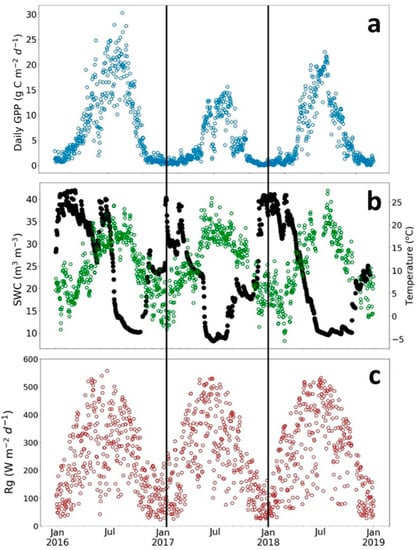
Figure 2.
Seasonal variation of daily sums of Gross Primary Productivity (Daily GPP) and meteorological variables for three growing seasons at the poplar plantation in Lochristi. (a) Daily GPP in gC m−2 d−1; (b) soil water content (SWC in m3 m−3, black dots) and air temperature (green dots); and (c) global radiation (Rg in W m−2 d−1).
The coppicing strongly reduced the photosynthetic activity of the SRC plantation in spring 2017 (Figure 2a). The maximum GPP was only half that in other years (15–30 g C m−2 d−1).
3.2. Describing SOS and EOS Using VIs
The three filtering methods applied to the raw data time-series produced different seasonal patterns (Figure 3). For GPP, the filters HANTS and SavGol described well the GPP pattern at SOS and EOS, while Polyfit did not perform well at EOS (Figure 3a). Furthermore, the HANTS filter captured best the GPP amplitude, and the SavGol filter followed best the interannual variability in GPP (Figure 3a). However, the estimates of phenological metrics of GPP showed a very small variability between years: day of the year (doy) 115 (SD ± 6) for SOS and doy 313 (SD ± 8) for EOS.
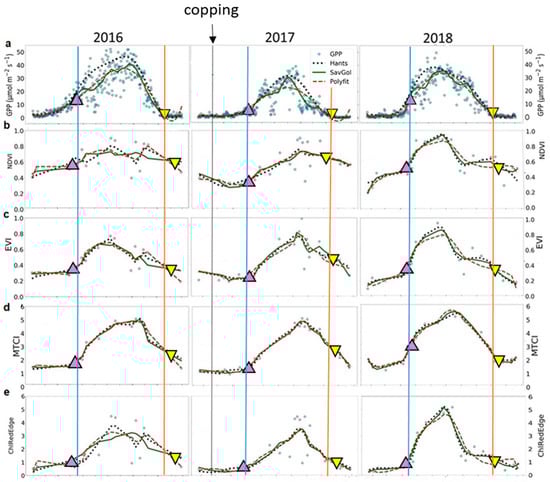
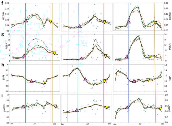
Figure 3.
Time-series of the seasonal variation of midday Gross Primary Productivity (GPP) and vegetation indices derived from Sentinel-2 images. (a) GPP (in μmol m−2 s−1); (b) NDVI—Normalized Difference Vegetation Index; (c) EVI—Enhanced Vegetation Index; (d) MTCI—MERIS Terrestrial Chlorophyll Index; and (e) ChlRedEdge—Chlorophyll red-edge; (f) MCARI—Modified Chlorophyll Absorption Ratio Index; (g) PSSR—Pigment Specific Simple Ratio; (h) SIPI—Structure Insensitive Pigment Index; (i) gNDVI—Green Normalized Difference Vegetation Index. Blue circles represent original data; dotted black lines represent HANTS series fitted data; green lines Savitzky–Golay (SavGol) series fitted data; and dashed red lines polynomial (Polyfit) series fitted data. Up-pointing pink and down-pointing yellow triangles represent mean values, in days, of the start and the end of season, respectively, derived from filtering methods. Blue and orange lines indicate the start and the end of season of GPP, respectively.
The coppicing in 2017 delayed the SOS of about ten days compared to 2018 (Figure 3a; doy 118 (SD ± 3) for 2016 and doy 108 (SD ± 1) for 2018). Very similar SOS dates were obtained for 2016 and 2017: doy 118 (SD ± 3) and doy 120 (SD ± 2) for 2017, respectively. The late start of the growing season in 2016 compared to 2018 related to the lower temperatures in spring (Figure 2b). The estimates of the EOS showed about a one-week difference between the 2016 (doy 320 SD ± 1) and 2017 (doy 313 SD ± 3) growing seasons and two weeks between the 2016 and 2018 growing seasons (doy 305 SD ± 5). The anticipated senescence in 2018 was linked to the low SWC in summer until the end of season (Figure 2b). The SWC recharge after the summer in 2017 prolonged the growing season in that year compared to 2018 (Figure 2b).
For VIs, the three filtering methods showed similar good performance in reproducing seasonal and interannual variability of GPP time-series at SOS (Table 3). The accuracy varied largely among VIs (Table 3, RMSE = 0.09—14.33 μmol m−2 s−1). Better performance in predicting GPP pattern at the SOS than at the EOS (Table 3, RMSE = 0.09—5.65 μmol m−2 s−1 for SOS and, RMSE = 1.12—14.33 μmol m−2 s−1 for EOS) was found. MTCI provided the best results in describing GPP phenology in 2016, ChlRedEdge in 2017 and MCARI predicted GPP well in 2018. Higher values of RMSE were found at EOS, except for MTCI in 2016 and in 2018 and EVI in 2017. Overall, HANTS and SavGol filters describe the GPP seasonality better than Polyfit at SOS and EOS, while HANTS and Polyfit performed slightly better at EOS.
Table 3.
Performance of each vegetation index (VI) and filtering methods (HANTS—Harmonic Analysis of Time Series; Polyfit—polynomial; SavGol—Savitzky–Golay) in simulating GPP time-series for each year and season (SOS—start of season; EOS—end of season), separately (see VI definitions in Table 1). RMSE—root mean squared error, in μmol m−2 s−1.
Scatter plots in Figure 4 shows the comparison between SOS derived from VIs and from GPP, grouped by year for threshold and filtering methods. The results of the same analysis applied to EOS are represented by scatter plots in Figure 5. A good performance in predicting SOS of GPP for all threshold methods and years was obtained for MTCI (Figure 4), points were the closest to the 1:1 line. For MCARI, NDVI, EVI and ChlRedEdge, the first derivative method failed in estimating SOS of GPP in 2016 for all filtering methods (Figure 4). Points for EOS for MTCI and EVI were the closest to the 1:1 line (Figure 5) indicating good performance in predicting EOS of GPP. Except for the first derivative method in 2016 and 2018, MCARI showed good performances too. Among other VIs, NDVI, gNDVI, ChlRedEdge and SIPI showed a clear tendency to predict the EOS later than GPP.
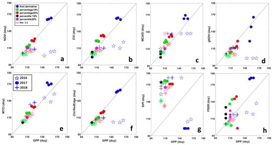
Figure 4.
Relationship between the start of the season (SOS), in days, derived from Gross Primary Productivity (GPP) and different vegetation indices. (a) NDVI—Normalized Difference Vegetation Index; (b) EVI—Enhanced Vegetation Index; (c) MCARI—Modified Chlorophyll Absorption Ratio Index; (d) gNDVI—Green Normalized Difference Vegetation Index; (e) MTCI—MERIS Terrestrial Chlorophyll Index; (f) ChlRedEdge—Chlorophyll red-edge; (g) SIPI—Structure Insensitive Pigment Index; and (h) PSSR—Pigment Specific Simple Ratio. Different colors represent different methods for deriving SOS: blue = first derivative method; green = percentage 10%; red = percentage 20%; black = percentile 10%; pink = percentile 20%. Symbols show different years: stars (☆) are for 2016; circles (●) for 2017 and plus (+) for 2018.
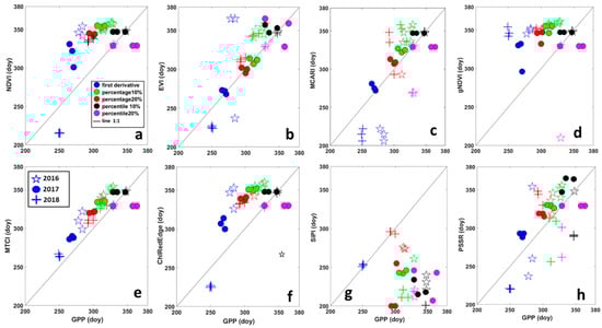
Figure 5.
Relationship between the end of the season (EOS), in days, derived from Gross Primary Productivity (GPP) and different vegetation indices. (a) NDVI—Normalized Difference Vegetation Index; (b) EVI—Enhanced Vegetation Index; (c) MCARI—Modified Chlorophyll Absorption Ratio Index; (d) gNDVI—Green Normalized Difference Vegetation Index; (e) MTCI—MERIS Terrestrial Chlorophyll Index; (f) ChlRedEdge—Chlorophyll red-edge; (g) SIPI—Structure Insensitive Pigment Index; and (h) PSSR—Pigment Specific Simple Ratio. Different colors represent different methods for deriving SOS: blue = first derivative method; green = percentage 10%; red = percentage 20%; black = percentile 10%; pink = percentile 20%. Symbols show different years: stars (☆) are for 2016; circles (●) for 2017 and plus (+) for 2018.
The analysis of the perpendicular distance to the 1:1 line confirmed that HANTS and Polyfit were the most suitable filtering methods for SOS, while for EOS it was not possible to identify only one method (Table 4). For SOS, the MTCI showed the minimum distance to 1:1 line (3.10 days (SD ± 3)), followed by ChlRedEdge (4.7 days), NDVI (5.08 days) and EVI (5.18 days). However, ChlRedEdge and NDVI showed very high variability (SD ± 4.23 and SD ± 4.25, respectively) among the different filtering methods (Figure 3 and Table 4). All other VIs showed larger distances, indicative of poor performance in predicting the SOS of GPP phenology. For EOS, MTCI and EVI showed a small distance to 1:1 line (10.41 days (SD ± 4.18) and 11.78 days (SD ± 5.48), respectively). Bigger distance values were found for other VIs (Table 4). Furthermore, the distance to the 1:1 line was VI-dependent and varied strongly with the filtering method (Table 4). However, the distance analysis confirmed that MTCI predicted well the SOS in 2016 (2.12 days (SD ± 1.81)) and the EOS in 2016 and 2018, the year with limiting SWC at the end of the growing season (Figure 3; 11.03 days (SD ± 2.49) and 6.59 days (SD ± 1.99), respectively). MCARI predicted well GPP at SOS in 2017 (the year of the copping; 1.37 days (SD ± 0.29), gNDVI (1.40 days (SD ± 0.84) at the SOS in 2018, while NDVI showed the best accuracy at the EOS in 2017 (7.68 days (SD ± 2.49; Figure 3, Table 4).
Table 4.
Distance, in days, to the 1:1 line between the start of the season (SOS) and the end of the season (EOS) derived from gross primary productivity (GPP) and VIs (see VIs definitions in Table 1) and for each filtering method (HANTS—Harmonic Analysis of Time Series; SavGol—Savitzky–Golay; and Polyfit—Polynomial). The shortest distances are in bold.
The 20% and 10% percentile were the best threshold for estimating GPP metrics for SOS. The distance between the EOS of GPP and EOS of VIs differed the least using a 10% percentile threshold (Table 5).
Table 5.
Distance, in days, to the 1:1 line between the start of the season (SOS) and the end of the season (EOS) derived from Gross Primary Productivity (GPP) and VIs (see VIs definitions in Table 1) and for each threshold method. The shortest distances are in bold.
Bar plots in Figure 6 show the difference between the SOS/EOS derived from GPP and the SOS/EOS derived from VIs for each year averaged for filtering methods. A positive difference illustrated an earlier SOS/EOS derived from VI time-series, while a negative difference was indicative of a delay in SOS/EOS. SIPI predicted more than one month later the SOS of GPP and about two months earlier the EOS of GPP. All VIs (except SIPI and MCARI) estimated the SOS earlier than GPP in 2016. MTCI showed the smallest difference with the SOS of GPP. This tendency to predict earlier the SOS of GPP was also evident for all VIs, except for MTCI, MCARI and SIPI, in 2018. PSSR predicted about 2 days earlier the SOS of GPP. For the 2017 growing season, the year of the copping, all VIs, except ChlRedEdge and gNDVI, delayed the SOS of GPP. NDVI showed the smallest difference with the SOS of GPP. Clearly, all VIs (except SIPI and MCARI in 2016, and SIPI in 2017) predicted later the EOS than the GPP for all years. The EOS predicted by EVI and MCARI, showed a smaller difference with the EOS of GPP in 2017 and 2018. PSSR differed little to EOS of the GPP in 2016.
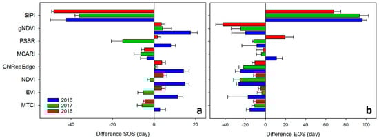
Figure 6.
Difference, in days, between phonological metrics derived from Gross Primary Productivity (GPP) and VIs (see VIs definitions in Table 1) for each year averaged for filtering methods. (a) SOS—start of season; (b) EOS—end of season. Error bars represent the standard deviation between the filtering method estimates.
The VIs performed differently in predicting daily GPP of the SRC plantation across the three growing seasons (Figure 6 and Supplementary material Figure S1). In addition, performances in predicting GPP also varied greatly across the years. MTCI performed best in predicting GPP for the 2016 and 2017 growing seasons (Figure 6) and for all three growing seasons together (R2 = 0.52, RMSE = 22.53 μmol m−2 s−1). In contrast, ChlRedEdge performed slightly better for the 2018 dry growing season (R2 = 0.59, RMSE = 22.86 μmol m−2 s−1). EVI showed a slightly lower performance than ChlRedEdge (R2 = 0.41, RMSE = 25.77 μmol m−2 s−1) while NDVI showed a poor performance in predicting GPP (R2 = 0.31, RMSE = 25.69 μmol m−2 s−1). All other VIs had limitations in predicting GPP seasonality (see Supplementary material Figure S1).
4. Discussion
This analysis explores for the first time the potential of using vegetation indices derived from the Sentinel-2 satellite for describing carbon flux phenology and productivity of SRC plantations.
4.1. GPP Phenology of SRC Plantations
The SRC plantation exhibited strong photosynthetic activity, in terms of GPP, until late in the season (Figure 2a). This was in line with previous studies on the same plantation reporting a net carbon uptake until the end of September [11,19], and on poplar trees [20]. Contrary to SRC plantations, a marked decline of net carbon uptake in early mid-September was observed in deciduous species [18]. The different growth strategy between SRC plantations and other deciduous species could be explained by a high allocation of nitrogen in leaves until late in the growing season, as reported for the same SRC plantation in Broeckx et al. (2014). In addition, in this SRC plantation, the production of new leaves quickly decreases around September [100].
The year-to-year variations in water and temperature regimes (Figure 2b) affected the phenology of the plantation (Figure 2 and Figure 3). Low temperatures in spring 2016 delayed the start of the growing season in that year. Low SWC at the end of season reduced GPP and anticipated the senescence in 2017 and 2018 (Figure 2). However, the SWC recharge after the summer in 2017 contributed to a delay at the end of the season in 2017 compared to 2018. Poplars show a high photosynthetic performance when SWC is not a limiting factor and GPP is controlled by a decrease in solar radiation and air temperature [17]. A reduction of photosynthetic activity under dry conditions might be caused by a decrease in leaf production and stomatal closure during dry periods [17].
Coppicing in 2017 had a distinct impact on GPP seasonality and interannual variability of the plantation (Figure 2). A delay in the start of the season was observed after copping and was documented for the same plantation in the previous study of Vanbeveren et al. (2016). After coppicing, poplars invest energy in the production of new buds from stumps, a process that delays the production of news leaves and the start of photosynthesis. However, this delay in the season start was counterbalanced by rapid growth and resprouting in subsequent growing seasons [101].
We found a delay of EOS in 2017 compared to 2018 and 2016, but there was no evidence that this delay was directly linked to copping. Based on this, and on previous studies reporting that coppicing does not affect autumn senescence [21], it is possible that SWC limitations might rather have contributed to the delay of EOS observed in 2017.
4.2. An Optimal Spectral Proxy for Describing GPP Phenology of SRC Plantations
Overall, our results revealed that MTCI was the most suitable proxy for describing the GPP phenology (i.e., it exhibited the lower distance in identifying the SOS- and EOS-dates (Table 4 and Table 5; Figure 4 and Figure 5), and the highest R² and lowest RMSE in reconstructing the seasonal pattern of GPP of the SRC plantation (Figure 7). MTCI described well the SOS and EOS in 2106 and detected well the EOS of the 2018 growing season (Figure 4 and Figure 5; Table 4). The estimates of phenological metrics derived from MTCI showed small differences with GPP phenology for all years anticipating the SOS and delaying the EOS. Among all other tested VIs SIPI and PSSR failed to reproduce the seasonal GPP pattern and to represent SOS and EOS of the GPP. We found that also EVI provided quite good estimates of SOS and EOS and seasonality of GPP, albeit in all cases lower performance than MTCI. NDVI, ChlRedEdge and MCARI performed a bit weaker than EVI, at both SOS and EOS. NDVI performed weaker than EVI, which performed weaker than ChlRedEdge in simulating GPP seasonal variability (Figure 7).
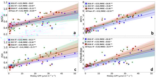
Figure 7.
Linear correlation between Gross Primary Productivity (GPP) and the vegetation indices. (a) NDVI—Normalized Vegetation Difference Index (NDVI); (b) EVI—Enhanced Vegetation Index; (c) MTCI—MERIS Terrestrial Chlorophyll Index; and (d) ChlRedEdge—chlorophyll red-edge index. The blue, green and red dots represent 2016, 2017 and 2018, respectively. The lines represent the linear fitted models. The shaded areas represent the 95% confidence intervals for the slopes of the fitted lines. R2, coefficient of determination; RMSE, root mean square error; * 0.01 < p ≤ 0.05; ** p ≤ 0.01.
MTCI is well known to be a reliable proxy of canopy chlorophyll content [35,52]. It has been successfully used as a proxy of GPP seasonal variability in several biomes [33,53,102,103,104,105]. Changes in canopy chlorophyll content play an important role in controlling ecosystem photosynthetic activity, i.e., GPP [49,105]. We observed an exceptionally good representation of the seasonal GPP pattern by MTCI (Figure 3, Table 3, Figure 7) [34,35,106]. This tight relationship between GPP and MTCI has been attributed to the fact that MTCI does not saturate at higher chlorophyll contents [69,107].
As expected, NDVI was not the best proxy for GPP (Table 4 and Table 5; Figure 7). NDVI index—such as the widely used “greenness indices”—has been demonstrated to be a good proxy of the fraction of absorbed photosynthetically active radiation (i.e., fAPAR) and LAI [108,109]. Changes in LAI among phenophases affect the shape of the relationship between NDVI and LAI that has almost linear trends during the growing season and declining during the senescence period [110,111]. NDVI shows limitations in describing seasonal LAI variations of dense canopies because it responds mainly to variations in the red and it is relatively insensitive to variations in the NIR [37,112]. These SRC plantations reached an LAI of about 10 in 2016 (data not shown), the last year of the third rotation, when the canopies were fully developed. The very high LAI in 2016 can explain the poor performance of NDVI for the SRC plantations. LAI of natural mature forests varies between 2 and 7 [37] and it could explain the better performance of NDVI in describing the phenology of deciduous forests. The same considerations can explain also the poor performance of other VIs calculated using the NIR reflectance (Table 1: SIPI, PSSR and gNDVI).
EVI is assumed to relate to green cover and, therefore, be a useful proxy for canopy phenology [113,114,115,116]. Other studies also reported that EVI well represents the seasonal patterns of GPP [42,117]. EVI was formulated to be less sensitive to atmospheric effects and reflection from soil than other greenness indices such as NDVI, by incorporating blue spectral wavelengths [118] to differentiate soil from vegetation [119].
The chlorophyll red-edge index (ChlRedEdge) is well recognized as a good proxy of chlorophyll content [120] and has been demonstrated to be a valuable descriptor of the seasonal changes in GPP [121]. Also in our study, ChlRedEdge showed good accuracy in predicting SOS and seasonality of GPP, albeit less than MTCI (refer to Table 4 and Table 5; Figure 7). Recently, it has been shown that the ChlRedEdge index can be a reliable proxy for leaf senescence as well for deciduous trees (i.e., European beech, pedunculate oak and silver birch) in the temperate zone [122]. However, this was not the case in our study, as ChlRedEdge did not provide a good estimation of EOS. It is important to note, however, that Mariën et al. (2019) focused on the onset of autumn senescence as identified by the breakpoint technique, whereas we used low percentiles and percentages, which correspond with the later stages of senescence, which could explain the different outcome between both studies. Coppicing strongly affects the canopy structure (i.e., leaf angle and distribution, orientation, leaf density) of the plantation modifying leaf light interception. These changes in canopy structure can strongly modify the spectral response of SRC plantations compared to natural deciduous forests. In addition, canopy structure can have a strong impact on the estimation of canopy nitrogen content [123]. During senescence, SRC plantations allocate a larger amount of nitrogen in leaves than deciduous forests. It could explain the different spectral responses of the SRC plantation compared to deciduous forests.
Sentinel-2 data are now systematically generated and the Level-2A product provides top of canopy reflectance images globally (https://earth.esa.int/web/sentinel/user-guides/sentinel-2-msi/product-types/level-2a). This permits to test the use of Sentinel-2 vegetation indices, in particular the MTCI, over other SRC plantations and different biomes. The recent ESA Sentinel-3 mission offers a unique set of data at the global scale with an improved spectral resolution of about 10 nm that may help to better understand plant traits and plant physiological status. The Sentinel-3 OLCI sensor covers the chlorophyll absorption region between 600 nm and 677 nm and the red-edge region between 697 nm and 755 nm. Sentinel-3 Level-1 OLCI products provide the so-called OLCI Terrestrial Chlorophyll Index (OTCI) which is a chlorophyll index that has the same formula of MTCI but it is calculated using the OLCI bands. OTCI is available at a spatial resolution of 300 m instead of the 20 m of Sentinel-2. Thus, the use of an approach similar to the one based on MTCI and presented here could contribute to the understanding of SRC phenology and GPP at a global scale.
4.3. Quality of Satellite Raw Data, Filtering and Threshold Methods
The filtering methods HANTS and Polyfit reproduced a better method for the seasonal and interannual variability of GPP of the SRC plantation (Figure 3; Table 3) than the SavGol method. Furthermore, both filtering methods were suitable for identifying the start and the end of carbon flux uptake (Table 4), as reported in previous studies [124]. Atkinson et al. (2012) [125] reported that fitting methods where each parameter of the fitting function is estimated by the least-square method are more robust. However, there is not a unique method that always performs better than another for filtering VI time-series [64].
The differences between the different filtering methods in reconstructing VI time-series could be related to their ability in detecting clouds and cloud shadow. The presence of clouds changes the optical properties of the signal. The cloud shadow weakens the light intensity and thus the reflectance of all bands is underestimated [64]. Furthermore, while the presence of clouds causes an underestimation of VIs, cloud shadow can lead to an overestimation of NDVI [64]. A limited description of the EOS in all years by most of the VIs could be also related to the large presence of clouds at the end of the summer and in autumn when senescence started (Figure 3, Table 4).
Another point worth mentioning relates to the accuracy of cloud masks used in the screening of clouds and cloud shadows. In this study, we used postprocessed Sentinel-2 data by Sen2Cor algorithm. The cloud classification generated by Sen2Cor shows limits in accurately identifying the cloud shadows. This classification does not reduce the noise of the time-series data but it produces a misleading classification of the satellite data quality. Therefore the remaining data with low quality but classified as good pixels might affect the patterns of fitted VI time-series (Figure 3, Table 3). The number of high-quality data of the time-series and their distribution in time affects the accuracy of the fitting functions [63]. A comparison of filtering methods is advisable, given their contrasting performance in the literature [64,89,125].
In addition to the quality of VI time-series and the robustness of the filtering functions, the accuracy of the phenophases also depends on the chosen detection method [126], i.e., the selected dates of SOS- and EOS occurrence depend on the thresholds that are chosen to represent them (Figure 4 and Figure 5). In this study, we found that for SOS, the dates at which the 10% and 20% percentile occurred showed very good agreement between VIs and the GPP data, while for EOS the dates of the 10% percentile came out as the best threshold (Table 5). The percentile method focuses on the position of the proxy for a fixed percentage (e.g., 10% and 20%). Several previous studies also obtained good results using such low percentiles as thresholds for determining the dates of SOS and EOS [127,128,129,130,131]. Furthermore, a threshold around 20% is good for estimating the start of greening [132]. Our analysis confirmed also that the extraction of phenological metrics from VI time-series is highly uncertain [65,66,67]. Combining multiple methods is preferred especially for estimating EOS dynamics (Table 5). The first derivative method is very sensitive to the noise in the signal and the temporal filtering and it cannot represent short growing seasons well, especially when the increase and decrease in the annual time-series occur rapidly and abruptly [133]. The percentage method is sensitive to the minimum and maximum values that may be affected by noise in the signal.
5. Conclusions
This study confirmed that VIs can be suitable estimators of the GPP phenology of SRC plantations and are able to detect the effect of coppicing on GPP. Among all investigated vegetation indices, MTCI showed the best fit with the GPP phenology. Additionally, the choice of the filtering method and the thresholds played an important role in defining the dates of SOS and EOS of GPP. These results open up a new possibility to estimate GPP of SRC plantations and should inspire new methods based on optical data for describing GPP and phenology.
Supplementary Materials
The following are available online at https://www.mdpi.com/2072-4292/12/13/2104/s1, Figure S1: Linear correlation between gross primary productivity (GPP) and the vegetation indices.
Author Contributions
M.M. performed all analyses and wrote the text; I.A.J. conceived and designed the experiment and wrote the text, J.M.B. contributed to remote sensing data processing; N.A. processed all eddy covariance data and wrote the text; M.B. conceived and designed the experiment, wrote the text, supervised the whole project and data analysis. M.M., N.A., J.M.B., S.W., Q.L., J.P., I.A.J. and M.B. contributed to discussions and revisions. All authors have read and agreed to the published version of the manuscript.
Funding
This research was funded by Belgian Science Policy Office (BELSPO) in the framework of the STEREO III program (ECOPROPHET project, contract number: SR/00/334). M.B. thanks the financial support provided by the European Union’s Horizon 2020 Research and Innovation program under the Marie Skłodowska-Curie grant (INDRO, grant agreement no. 702717).
Acknowledgments
Authors gratefully acknowledge the technical assistance of Jan Segers in the field.
Conflicts of Interest
The authors declare no conflict of interest.
References
- McEwan, A.; Marchi, E.; Spinelli, R.; Brink, M. Past, present and future of industrial plantation forestry and implication on future timber harvesting technology. J. For. Res. 2020, 31, 339–351. [Google Scholar] [CrossRef]
- Al Afas, N.; Marron, N.; Ceulemans, R. Clonal variation in stomatal characteristics related to biomass production of 12 poplar (populus) clones in a short rotation coppice culture. Environ. Exp. Bot. 2006, 58, 279–286. [Google Scholar] [CrossRef]
- Hall, D.O.; Scrase, J.I. Will biomass be the environmentally friendly fuel of the future? Biomass Bioenergy 1998, 15, 357–367. [Google Scholar] [CrossRef]
- Verheyen, K.; Buggenhout, M.; Vangansbeke, P.; De Dobbelaere, A.; Verdonckt, P.; Bonte, D. Potential of short rotation coppice plantations to reinforce functional biodiversity in agricultural landscapes. Biomass Bioenergy 2014, 67, 435–442. [Google Scholar] [CrossRef]
- Don, A.; Osborne, B.; Hastings, A.; Skiba, U.; Carter, M.S.; Drewer, J.; Flessa, H.; Freibauer, A.; Hyvönen, N.; Jones, M.B.; et al. Land-use change to bioenergy production in europe: Implications for the greenhouse gas balance and soil carbon. GCB Bioenergy 2012, 4, 372–391. [Google Scholar] [CrossRef]
- Berhongaray, G.; Verlinden, M.S.; Broeckx, L.S.; Janssens, I.A.; Ceulemans, R. Soil carbon and belowground carbon balance of a short-rotation coppice: Assessments from three different approaches. GCB Bioenergy 2017, 9, 299–313. [Google Scholar] [CrossRef] [PubMed]
- Dimitriou, I.; Busch, G.; Jacobs, S.; Schmidt-Walter, P.; Lamersdorf, N. A review of the impacts of short rotation coppice cultivation on water issues. Agric. For. Res. 2009, 3, 197–206. [Google Scholar]
- UN/ECE-FAO. Forest Resources of Europe, Cis, North America, Australia, Japan and New Zealand. Main Report; Timber and forest study papers 17; United Nations Publication: Geneva, Switzerland, 2000. [Google Scholar]
- FAO. Poplars and Other Fast-Growing Trees-Renewable Resources for Future Green Economies; Forestry Policy and Resources Division; FAO: Rome, Italy, 13–16 September 2016. [Google Scholar]
- Pietrzykowski, M.; Woś, B.; Tylek, P.; Kwaśniewski, D.; Juliszewski, T.; Walczyk, J.; Likus-Cieślik, J.; Ochał, W.; Tabor, S. Carbon sink potential and allocation in above- and below-ground biomass in willow coppice. J. For. Res. 2020. [Google Scholar] [CrossRef]
- Horemans, J.A.; Arriga, N.; Ceulemans, R. Greenhouse gas budget of a poplar bioenergy plantation in belgium: Co2 uptake outweighs ch4 and n2o emissions. GCB Bioenergy 2019, 11, 1435–1443. [Google Scholar] [CrossRef]
- Richardson, A.D.; Black, T.A.; Ciais, P.; Delbart, N.; Friedl, M.A.; Gobron, N.; Hollinger, D.Y.; Kutsch, W.L.; Longdoz, B.; Luyssaert, S.; et al. Influence of spring and autumn phenological transitions on forest ecosystem productivity. Philos. Trans. R. Soc. Lond. Ser. B Biol. Sci. 2010, 365, 3227–3246. [Google Scholar] [CrossRef]
- Churkina, G.; Schimel, D.; Braswell, B.H.; Xiao, X. Spatial analysis of growing season length control over net ecosystem exchange. Glob. Chang. Biol. 2005, 11, 1777–1787. [Google Scholar] [CrossRef]
- Black, T.A.; Chen, W.J.; Barr, A.G.; Arain, M.A.; Chen, Z.; Nesic, Z.; Hogg, E.H.; Neumann, H.H.; Yang, P.C. Increased carbon sequestration by a boreal deciduous forest in years with a warm spring. Geophys. Res. Lett. 2000, 27, 1271–1274. [Google Scholar] [CrossRef]
- Griffis, T.J.; Black, T.A.; Gaumont-Guay, D.; Drewitt, G.B.; Nesic, Z.; Barr, A.G.; Morgenstern, K.; Kljun, N. Seasonal variation and partitioning of ecosystem respiration in a southern boreal aspen forest. Agric. For. Meteorol. 2004, 125, 207–223. [Google Scholar] [CrossRef]
- Campioli, M.; Gielen, B.; Goeckede, M.; Papale, D.; Bouriaud, O.; Granier, A. Temporal variability of the npp-gpp ratio at seasonal and interannual time scales in a temperate beech forest. Biogeosciences 2011, 8, 2481–2492. [Google Scholar] [CrossRef]
- Broeckx, L.S.; Verlinden, M.S.; Berhongaray, G.; Zona, D.; Fichot, R.; Ceulemans, R. The effect of a dry spring on seasonal carbon allocation and vegetation dynamics in a poplar bioenergy plantation. GCB Bioenergy 2014, 6, 473–487. [Google Scholar] [CrossRef]
- Wilson, K.B.; Baldocchi, D.D.; Hanson, P.J. Spatial and seasonal variability of photosynthetic parameters and their relationship to leaf nitrogen in a deciduous forest. Tree Physiol. 2000, 20, 565–578. [Google Scholar] [CrossRef]
- Zona, D.; Janssens, I.A.; Aubinet, M.; Gioli, B.; Vicca, S.; Fichot, R.; Ceulemans, R. Fluxes of the greenhouse gases (co2, ch4 and n2o) above a short-rotation poplar plantation after conversion from agricultural land. Agric. For. Meteorol. 2013, 169, 100–110. [Google Scholar] [CrossRef]
- Bernacchi, C.J.; Calfapietra, C.; Davey, P.A.; Wittig, V.E.; Scarascia-Mugnozza, G.E.; Raines, C.A.; Long, S.P. Photosynthesis and stomatal conductance responses of poplars to free-air co2 enrichment (popface) during the first growth cycle and immediately following coppice. New Phytol. 2003, 159, 609–621. [Google Scholar] [CrossRef]
- Pellis, A.; Laureysens, I.; Ceulemans, R. Growth and production of a short rotation coppice culture of poplar i. Clonal differences in leaf characteristics in relation to biomass production. Biomass Bioenergy 2004, 27, 9–19. [Google Scholar] [CrossRef]
- Vanbeveren, S.P.P.; Bloemen, J.; Balzarolo, M.; Broeckx, L.S.; Sarzi-Falchi, I.; Verlinden, M.S.; Ceulemans, R. A comparative study of four approaches to assess phenology of populus in a short-rotation coppice culture. iForest 2016, 9, 682–689. [Google Scholar] [CrossRef]
- Aubinet, M.; Grelle, A.; Ibrom, A.; Rannik, Ü.; Moncrieff, J.; Foken, T.; Kowalski, A.S.; Martin, P.; Berbigier, P.; Bernhofer, C.; et al. Estimates of the annual net carbon and water exchange of forests: The euroflux methodology. Adv. Ecol Res 2000, 30, 113–175. [Google Scholar]
- Baldocchi, D.; Chu, H.; Reichstein, M. Inter-annual variability of net and gross ecosystem carbon fluxes: A review. Agric. For. Meteorol. 2018, 249, 520–533. [Google Scholar] [CrossRef]
- Baldocchi, D.; Penuelas, J. The physics and ecology of mining carbon dioxide from the atmosphere by ecosystems. Glob. Chang. Biol. 2019, 25, 1191–1197. [Google Scholar] [CrossRef] [PubMed]
- Arriga, N.; Rannik, Ü.; Aubinet, M.; Carrara, A.; Vesala, T.; Papale, D. Experimental validation of footprint models for eddy covariance co2 flux measurements above grassland by means of natural and artificial tracers. Agric. For. Meteorol. 2017, 242, 75–84. [Google Scholar] [CrossRef]
- Liu, Q.; Fu, Y.S.H.; Zhu, Z.C.; Liu, Y.W.; Liu, Z.; Huang, M.T.; Janssens, I.A.; Piao, S.L. Delayed autumn phenology in the northern hemisphere is related to change in both climate and spring phenology. Glob. Chang. Biol. 2016, 22, 3702–3711. [Google Scholar] [CrossRef] [PubMed]
- Piao, S.; Fang, J.; Zhou, L.; Ciais, P.; Zhu, B. Variations in satellite-derived phenology in china’s temperate vegetation. Glob. Chang. Biol. 2006, 12, 672–685. [Google Scholar] [CrossRef]
- Blackburn, G.A. Quantifying chlorophylls and caroteniods at leaf and canopy scales: An evaluation of some hyperspectral approaches. Remote Sens. Environ. 1998, 66, 273–285. [Google Scholar] [CrossRef]
- Rahman, A.F.; Sims, D.A.; Cordova, V.D.; El-Masri, B.Z. Potential of modis evi and surface temperature for directly estimating per-pixel ecosystem c fluxes. Geophys. Res. Lett. 2005, 32. [Google Scholar] [CrossRef]
- Sims, D.A.; Rahman, A.F.; Cordova, V.D.; El-Masri, B.Z.; Baldocchi, D.D.; Flanagan, L.B.; Goldstein, A.H.; Hollinger, D.Y.; Misson, L.; Monson, R.K.; et al. On the use of modis evi to assess gross primary productivity of north american ecosystems. J. Geophys. Res.-Biogeosci. 2006, 111, 16. [Google Scholar] [CrossRef]
- Saleska, S.R.; Didan, K.; Huete, A.R.; da Rocha, H.R. Amazon forests green-up during 2005 drought. Science 2007, 318, 612. [Google Scholar] [CrossRef]
- Wu, C.; Niu, Z.; Tang, Q.; Huang, W.; Rivard, B.; Feng, J. Remote estimation of gross primary production in wheat using chlorophyll-related vegetation indices. Agric. For. Meteorol. 2009, 149, 1015–1021. [Google Scholar] [CrossRef]
- Balzarolo, M.; Vescovo, L.; Hammerle, A.; Gianelle, D.; Papale, D.; Tomelleri, E.; Wohlfahrt, G. On the relationship between ecosystem-scale hyperspectral reflectance and CO2 exchange in European mountain grasslands. Biogeosciences 2015, 12, 3089–3108. [Google Scholar] [CrossRef]
- Rossini, M.; Cogliati, S.; Meroni, M.; Migliavacca, M.; Galvagno, M.; Busetto, L.; Cremonese, E.; Julitta, T.; Siniscalco, C.; Morra di Cella, U.; et al. Remote sensing-based estimation of gross primary production in a subalpine grassland. Biogeosciences 2012, 9, 2565–2584. [Google Scholar] [CrossRef]
- Rouse, J.W., Jr.; Haas, R.H.; Schell, J.A.; Deering, D.W. Monitoring Vegetation Systems in the Great Plains with ERTS. 1974. Available online: https://ntrs.nasa.gov/archive/nasa/casi.ntrs.nasa.gov/19740022614.pdf (accessed on 9 June 2020).
- Huete, A.R.; Liu, H.Q.; Batchily, K.; van Leeuwen, W. A comparison of vegetation indices over a global set of tm images for eos-modis. Remote Sens. Environ. 1997, 59, 440–451. [Google Scholar] [CrossRef]
- Loranty, M.M.; Davydov, S.P.; Kropp, H.; Alexander, H.D.; Mack, M.C.; Natali, S.M.; Zimov, N.S. Vegetation indices do not capture forest cover variation in upland siberian larch forests. Remote Sens. 2018, 10, 1686. [Google Scholar] [CrossRef]
- Wu, C.; Han, X.; Ni, J.; Niu, Z.; Huang, W. Estimation of gross primary production in wheat from in situ measurements. Int. J. Appl. Earth Obs. Geoinf. 2010, 12, 183–189. [Google Scholar] [CrossRef]
- Peng, Y.; Gitelson, A.A. Remote estimation of gross primary productivity in soybean and maize based on total crop chlorophyll content. Remote Sens. Environ. 2012, 117, 440–448. [Google Scholar] [CrossRef]
- Reed, B.C.; Brown, J.F.; VanderZee, D.; Loveland, T.R.; Merchant, J.W.; Ohlen, D.O. Measuring phenological variability from satellite imagery. J. Veg. Sci. 1994, 5, 703–714. [Google Scholar] [CrossRef]
- Huete, A.; Didan, K.; Miura, T.; Rodriguez, E.P.; Gao, X.; Ferreira, L.G. Overview of the radiometric and biophysical performance of the modis vegetation indices. Remote Sens. Environ. 2002, 83, 195–213. [Google Scholar] [CrossRef]
- Suzuki, R.; Nomaki, T.; Yasunari, T. West–east contrast of phenology and climate in northern asia revealed using a remotely sensed vegetation index. Int. J. Biometeorol. 2003, 47, 126–138. [Google Scholar] [CrossRef]
- Balzarolo, M.; Peñuelas, J.; Veroustraete, F. Influence of landscape heterogeneity and spatial resolution in multi-temporal in situ and modis ndvi data proxies for seasonal GPP dynamics. Remote Sens. 2019, 11, 1656. [Google Scholar] [CrossRef]
- Karkauskaite, P.; Tagesson, T.; Fensholt, R. Evaluation of the plant phenology index (ppi), ndvi and evi for start-of-season trend analysis of the northern hemisphere boreal zone. Remote Sens. 2017, 9, 485. [Google Scholar] [CrossRef]
- Vicca, S.; Balzarolo, M.; Filella, I.; Granier, A.; Herbst, M.; Knohl, A.; Longdoz, B.; Mund, M.; Nagy, Z.; Pinter, K.; et al. Remotely-sensed detection of effects of extreme droughts on gross primary production. Sci. Rep. 2016, 6, 28269. [Google Scholar] [CrossRef]
- Gamon, J.A.; Huemmrich, K.F.; Wong, C.Y.S.; Ensminger, I.; Garrity, S.; Hollinger, D.Y.; Noormets, A.; Peñuelas, J. A remotely sensed pigment index reveals photosynthetic phenology in evergreen conifers. Proc. Natl. Acad. Sci. USA 2016, 113, 13087. [Google Scholar] [CrossRef] [PubMed]
- Ulsig, L.; Nichol, C.; Huemmrich, K.; Landis, D.; Middleton, E.; Lyapustin, A.; Mammarella, I.; Levula, J.; Porcar-Castell, A. Detecting inter-annual variations in the phenology of evergreen conifers using long-term modis vegetation index time series. Remote Sens. 2017, 9, 49. [Google Scholar] [CrossRef]
- Gitelson, A.A.; Viña, A.; Verma, S.B.; Rundquist, D.C.; Arkebauer, T.J.; Keydan, G.; Leavitt, B.; Ciganda, V.; Burba, G.G.; Suyker, A.E. Relationship between gross primary production and chlorophyll content in crops: Implications for the synoptic monitoring of vegetation productivity. J. Geophys. Res. Atmos. 2006, 111. [Google Scholar] [CrossRef]
- Gitelson, A.A.; Stark, R.; Grits, U.; Rundquist, D.; Kaufman, Y.; Derry, D. Vegetation and soil lines in visible spectral space: A concept and technique for remote estimation of vegetation fraction. Int. J. Remote Sens. 2002, 23, 2537–2562. [Google Scholar] [CrossRef]
- Wang, F.-M.; Huang, J.-F.; Tang, Y.-L.; Wang, X.-Z. New vegetation index and its application in estimating leaf area index of rice. Rice Sci. 2007, 14, 195–203. [Google Scholar] [CrossRef]
- Gitelson, A.A.; Merzlyak, M.N.; Lichtenthaler, H.K. Detection of red edge position and chlorophyll content by reflectance measurements near 700 nm. J. Plant Physiol. 1996, 148, 501–508. [Google Scholar] [CrossRef]
- Dash, J.; Jeganathan, C.; Atkinson, P.M. The use of meris terrestrial chlorophyll index to study spatio-temporal variation in vegetation phenology over india. Remote Sens. Environ. 2010, 114, 1388–1402. [Google Scholar] [CrossRef]
- Zhang, W.; Liu, T.; Ren, G.; Hörtensteiner, S.; Zhou, Y.; Cahoon, E.B.; Zhang, C. Chlorophyll degradation: The tocopherol biosynthesis-related phytol hydrolase in arabidopsis seeds is still missing. Plant Physiol. 2014, 166, 70. [Google Scholar] [CrossRef] [PubMed]
- Liu, D.W.; Song, K.S.; Zhang, B.; Li, F.; IEEE. Hyperspectral Approaches for Detecting the Roadside Tree Chlorophyll Content with bp Neural Networks. In Proceedings. 2005 IEEE International Geoscience and Remote Sensing Symposium; IEEE: New York, NY, USA, 2005; pp. 3032–3035. [Google Scholar]
- Blackburn, G.A. Relationships between spectral reflectance and pigment concentrations in stacks of deciduous broadleaves. Remote Sens. Environ. 1999, 70, 224–237. [Google Scholar] [CrossRef]
- Haboudane, D.; Miller, J.R.; Tremblay, N.; Zarco-Tejada, P.J.; Dextraze, L. Integrated narrow-band vegetation indices for prediction of crop chlorophyll content for application to precision agriculture. Remote Sens. Environ. 2002, 81, 416–426. [Google Scholar] [CrossRef]
- Wu, C.; Niu, Z.; Tang, Q.; Huang, W. Estimating chlorophyll content from hyperspectral vegetation indices: Modeling and validation. Agric. For. Meteorol. 2008, 148, 1230–1241. [Google Scholar] [CrossRef]
- Peñuelas, J.; Filella, I.; Lloret, P.; Munoz, F.; Vilajeliu, M. Reflectance assessment of mite effects on apple-trees. Int. J. Remote Sens. 1995, 16, 2727–2733. [Google Scholar] [CrossRef]
- Peñuelas, J.; Filella, I. Visible and near-infrared reflectance techniques for diagnosing plant physiological status. Trends Plant Sci. 1998, 3, 151–3156. [Google Scholar] [CrossRef]
- Fusaro, L.; Salvatori, E.; Mereu, S.; Manes, F. Photosynthetic traits as indicators for phenotyping urban and peri-urban forests: A case study in the metropolitan city of rome. Ecol. Indic. 2019, 103, 301–311. [Google Scholar] [CrossRef]
- Bórnez, K.; Descals, A.; Verger, A.; Peñuelas, J. Land surface phenology from vegetation and proba-v data. Assessment over deciduous forests. Int. J. Appl. Earth Obs. Geoinf. 2020, 84, 101974. [Google Scholar] [CrossRef]
- Jönsson, P.; Cai, Z.; Melaas, E.; Friedl, M.A.; Eklundh, L. A method for robust estimation of vegetation seasonality from landsat and sentinel-2 time series data. Remote Sens. 2018, 10, 635. [Google Scholar] [CrossRef]
- Cai, Z.; Jönsson, P.; Jin, H.; Eklundh, L. Performance of smoothing methods for reconstructing ndvi time-series and estimating vegetation phenology from modis data. Remote Sens. 2017, 9, 1271. [Google Scholar] [CrossRef]
- Liu, Q.; Fu, Y.H.; Zeng, Z.; Huang, M.; Li, X.; Piao, S. Temperature, precipitation, and insolation effects on autumn vegetation phenology in temperate China. Glob. Chang. Biol. 2016, 22, 644–656. [Google Scholar] [CrossRef]
- Zhang, Q.; Kong, D.; Shi, P.; Singh, V.P.; Sun, P. Vegetation phenology on the qinghai-tibetan plateau and its response to climate change (1982–2013). Agric. For. Meteorol. 2018, 248, 408–417. [Google Scholar] [CrossRef]
- Solano-Correa, Y.T.; Bovolo, F.; Bruzzone, L.; Fernández-Prieto, D. Automatic derivation of cropland phenological parameters by adaptive non-parametric regression of sentinel-2 ndvi time series. In IGARSS 2018–2018 IEEE International Geoscience and Remote Sensing Symposium; IEEE: Piscataway, NJ, USA, 2018; pp. 1946–1949. [Google Scholar]
- Rouse, J.W.; Haas, R.H.; Schell, J.A.; Deering, D.W. Monitoring Vegetation Systems in the Great Plains with Erts; Freden, S.C., Mercanti, E.P., Becker, M., Eds.; Third Earth Resources Technology Satellite–1 Symposium, NASA SP-353; US Government Printing Office: Washington, DC, USA, 1974; Volume 1.
- Dash, J.; Curran, P.J. The meris terrestrial chlorophyll index. Int. J. Remote Sens. 2004, 25, 5403–5413. [Google Scholar] [CrossRef]
- Gleason, W.B.; Fu, Z.; Birktoft, J.; Banaszak, L. Refined crystal structure of mitochondrial malate dehydrogenase from porcine heart and the consensus structure for dicarboxylic acid oxidoreductases. Biochemistry 1994, 33, 2078–2088. [Google Scholar] [CrossRef] [PubMed]
- Rad, A.M.; Ashourloo, D.; Shahrabi, H.S.; Nematollahi, H. Developing an automatic phenology-based algorithm for rice detection using sentinel-2 time-series data. IEEE J. Sel. Top. Appl. Earth Obs. Remote Sens. 2019, 12, 1471–1481. [Google Scholar]
- Pinzon, J.E.; Tucker, C.J. A non-stationary 1981–2012 avhrr ndvi3g time series. Remote Sens. 2014, 6, 6929–6960. [Google Scholar] [CrossRef]
- Darvishzadeh, R.; Wang, T.J.; Skidmore, A.; Vrieling, A.; O’Connor, B.; Gara, T.W.; Ens, B.J.; Paganini, M. Analysis of sentinel-2 and rapideye for retrieval of leaf area index in a saltmarsh using a radiative transfer model. Remote Sens. 2019, 11, 671. [Google Scholar] [CrossRef]
- Feilhauer, H.; Schmid, T.; Faude, U.; Sánchez-Carrillo, S.; Cirujano, S. Are remotely sensed traits suitable for ecological analysis? A case study of long-term drought effects on leaf mass per area of wetland vegetation. Ecol. Indic. 2018, 88, 232–240. [Google Scholar] [CrossRef]
- Broeckx, L.S.; Verlinden, M.S.; Ceulemans, R. Establishment and two-year growth of a bio-energy plantation with fast-growing populus trees in flanders (belgium): Effects of genotype and former land use. Biomass Bioenergy 2012, 42, 151–163. [Google Scholar] [CrossRef]
- Verlinden, M.S.; Broeckx, L.S.; Ceulemans, R. First vs. Second rotation of a poplar short rotation coppice: Above-ground biomass productivity and shoot dynamics. Biomass Bioenergy 2015, 73, 174–185. [Google Scholar] [CrossRef]
- Aubinet, M.; Vesala, T.; Papale, D. Eddy Covariance: A Practical Guide to Measurement and Data Analysis; Springer: Dordrecht, The Netherlands, 2012. [Google Scholar]
- Pita, G.; Gielen, B.; Zona, D.; Rodrigues, A.; Rambal, S.; Janssens, I.A.; Ceulemans, R. Carbon and water vapor fluxes over four forests in two contrasting climatic zones. Agric. For. Meteorol. 2013, 180, 211–224. [Google Scholar] [CrossRef]
- Fratini, G.; McDermitt, D.K.; Papale, D. Eddy-covariance flux errors due to biases in gas concentration measurements: Origins, quantification and correction. Biogeosciences 2014, 11, 1037–1051. [Google Scholar] [CrossRef]
- Reichstein, M.; Falge, E.; Baldocchi, D.; Papale, D.; Aubinet, M.; Berbigier, P.; Bernhofer, C.; Buchmann, N.; Gilmanov, T.; Granier, A.; et al. On the separation of net ecosystem exchange into assimilation and ecosystem respiration: Review and improved algorithm. Glob. Chang. Biol. 2005, 11, 1424–1439. [Google Scholar] [CrossRef]
- Lasslop, G.; Reichstein, M.; Papale, D.; Richardson, A.D.; Arneth, A.; Barr, A.; Stoy, P.; Wohlfahrt, G. Separation of net ecosystem exchange into assimilation and respiration using a light response curve approach: Critical issues and global evaluation. Glob. Chang. Biol. 2010, 16, 187–208. [Google Scholar] [CrossRef]
- Barrios, J.M.; Meulenberghs-Gellens, F.; Hamdi, F.; Wieneke, S.; Janssens, I.; Balzarolo, M. Landscape heterogeneity around flux measurement stations investigated through sentinel-2 and proba-v satellite imagery. In Remote Sensing for Agriculture, Ecosystems, and Hydrology xx; Neale, C.M.U., Maltese, A., Eds.; SPIE-International Society Optical Engineering: Bellingham, WA, USA, 2018; Volume 10783. [Google Scholar]
- Jonsson, P.; Eklundh, L. Seasonality extraction by function fitting to time-series of satellite sensor data. Geosci. Remote Sens. IEEE Trans. 2002, 40, 1824–1832. [Google Scholar] [CrossRef]
- Chen, J.; Jönsson, P.; Tamura, M.; Gu, Z.; Matsushita, B.; Eklundh, L. A simple method for reconstructing a high-quality ndvi time-series data set based on the savitzky–golay filter. Remote Sens. Environ. 2004, 91, 332–344. [Google Scholar] [CrossRef]
- Kandasamy, S.; Baret, F.; Verger, A.; Neveux, P.; Weiss, M. A comparison of methods for smoothing and gap filling time series of remote sensing observations – application to modis lai products. Biogeosciences 2013, 10, 4055–4071. [Google Scholar] [CrossRef]
- Savitzky, A.; Golay, M.J.E. Smoothing and differentiation of data by simplified least squares procedures. Anal. Chem. 1964, 36, 1627–1639. [Google Scholar] [CrossRef]
- Menenti, M.; Azzali, S.; Verhoef, W. Fourier analysis of time series of noaa-avhrr ndvi composites to map isogrowth zones. In Studies in Environmental Science; Zwerver, S., van Rompaey, R.S.A.R., Kok, M.T.J., Berk, M.M., Eds.; Elsevier: Amsterdam, The Netherlands, 1995; Volume 65, pp. 425–430. [Google Scholar]
- Verhoef, W.; Menenti, M.; Azzali, S. Cover a colour composite of noaa-avhrr-ndvi based on time series analysis (1981–1992). Int. J. Remote Sens. 1996, 17, 231–235. [Google Scholar] [CrossRef]
- White, M.A.; de Beurs, K.M.; Didan, K.; Inouye, D.W.; Richardson, A.D.; Jensen, O.P.; O’Keefe, J.; Zhang, G.; Nemani, R.R.; van Leeuwen, W.J.D.; et al. Intercomparison, interpretation, and assessment of spring phenology in north america estimated from remote sensing for 1982–2006. Glob. Chang. Biol. 2009, 15, 2335–2359. [Google Scholar] [CrossRef]
- Zhang, X.; Friedl, M.A.; Schaaf, C.B.; Strahler, A.H.; Hodges, J.C.F.; Gao, F.; Reed, B.C.; Huete, A. Monitoring vegetation phenology using modis. Remote Sens. Environ. 2003, 84, 471–475. [Google Scholar] [CrossRef]
- Soudani, K.; le Maire, G.; Dufrêne, E.; François, C.; Delpierre, N.; Ulrich, E.; Cecchini, S. Evaluation of the onset of green-up in temperate deciduous broadleaf forests derived from moderate resolution imaging spectroradiometer (modis) data. Remote Sens. Environ. 2008, 112, 2643–2655. [Google Scholar] [CrossRef]
- Moulin, S.; Kergoat, L.; Viovy, N.; Dedieu, G. Global-scale assessment of vegetation phenology using noaa/avhrr satellite measurements. J. Clim. 1997, 10, 1154–1170. [Google Scholar] [CrossRef]
- Zheng, H.; Cheng, T.; Yao, X.; Deng, X.; Tian, Y.; Cao, W.; Zhu, Y. Detection of rice phenology through time series analysis of ground-based spectral index data. Field Crop. Res. 2016, 198, 131–139. [Google Scholar] [CrossRef]
- Shen, S.S.P.; Yin, H.; Cannon, K.; Howard, A.; Chetner, S.; Karl, T.R. Temporal and spatial changes of the agroclimate in alberta, canada, from 1901 to 2002. J. Appl. Meteorol. 2005, 44, 1090–1105. [Google Scholar] [CrossRef]
- Gordo, O.; Tryjanowski, P.; Kosicki, J.Z.; Fulin, M. Complex phenological changes and their consequences in the breeding success of a migratory bird, the white stork ciconia ciconia. J. Anim. Ecol. 2013, 82, 1072–1085. [Google Scholar] [CrossRef]
- Jain, P.; Wang, X.L.; Flannigan, M.D. Trend analysis of fire season length and extreme fire weather in north america between 1979 and 2015. Int. J. Wildland Fire 2017, 26, 1009–1020. [Google Scholar] [CrossRef]
- Bandoc, G.; Prăvălie, R.; Patriche, C.; Dragomir, E.; Tomescu, M. Response of phenological events to climate warming in the southern and south-eastern regions of romania. Stoch. Environ. Res. Risk Assess. 2018, 32, 1113–1129. [Google Scholar] [CrossRef]
- Jeong, S.-J.; Schimel, D.; Frankenberg, C.; Drewry, D.T.; Fisher, J.B.; Verma, M.; Berry, J.A.; Lee, J.-E.; Joiner, J. Application of satellite solar-induced chlorophyll fluorescence to understanding large-scale variations in vegetation phenology and function over northern high latitude forests. Remote Sens. Environ. 2017, 190, 178–187. [Google Scholar] [CrossRef]
- Gao, F.; Anderson, M.C.; Zhang, X.; Yang, Z.; Alfieri, J.G.; Kustas, W.P.; Mueller, R.; Johnson, D.M.; Prueger, J.H. Toward mapping crop progress at field scales through fusion of landsat and modis imagery. Remote Sens. Environ. 2017, 188, 9–25. [Google Scholar] [CrossRef]
- Broeckx, L.S.; Fichot, R.; Verlinden, M.S.; Ceulemans, R. Seasonal variations in photosynthesis, intrinsic water-use efficiency and stable isotope composition of poplar leaves in a short-rotation plantation. Tree Physiol. 2014, 34, 701–715. [Google Scholar] [CrossRef] [PubMed]
- Vanbeveren, S.P.P.; Ceulemans, R. Genotypic differences in biomass production during three rotations of short-rotation coppice. Biomass Bioenergy 2018, 119, 198–205. [Google Scholar] [CrossRef]
- Peng, Y.; Gitelson, A.A.; Keydan, G.; Rundquist, D.C.; Moses, W. Remote estimation of gross primary production in maize and support for a new paradigm based on total crop chlorophyll content. Remote Sens. Environ. 2011, 115, 978–989. [Google Scholar] [CrossRef]
- Gitelson, A.A.; Peng, Y.; Masek, J.G.; Rundquist, D.C.; Verma, S.; Suyker, A.; Baker, J.M.; Hatfield, J.L.; Meyers, T. Remote estimation of crop gross primary production with landsat data. Remote Sens. Environ. 2012, 121, 404–414. [Google Scholar] [CrossRef]
- Harris, A.; Dash, J. A new approach for estimating northern peatland gross primary productivity using a satellite-sensor-derived chlorophyll index. J. Geophys. Res. Biogeosci. 2011, 116. [Google Scholar] [CrossRef]
- Zhang, S.; Liu, L.Y. The potential of the meris terrestrial chlorophyll index for crop yield prediction. Remote Sens. Lett. 2014, 5, 733–742. [Google Scholar] [CrossRef]
- Sakowska, K.; Vescovo, L.; Marcolla, B.; Juszczak, R.; Olejnik, J.; Gianelle, D. Monitoring of carbon dioxide fluxes in a subalpine grassland ecosystem of the italian alps using a multispectral sensor. Biogeosciences 2014, 11, 4695–4712. [Google Scholar] [CrossRef]
- Dash, J.; Curran, P.J. Evaluation of the meris terrestrial chlorophyll index (mtci). Adv. Space Res. 2007, 39, 100–104. [Google Scholar] [CrossRef]
- Hmimina, G.; Dufrene, E.; Soudani, K. Relationship between photochemical reflectance index and leaf ecophysiological and biochemical parameters under two different water statuses: Towards a rapid and efficient correction method using real-time measurements. Plant Cell Enviorn. 2014, 37, 473–487. [Google Scholar] [CrossRef] [PubMed]
- Soudani, K.; Hmimina, G.; Dufrêne, E.; Berveiller, D.; Delpierre, N.; Ourcival, J.-M.; Rambal, S.; Joffre, R. Relationships between photochemical reflectance index and light-use efficiency in deciduous and evergreen broadleaf forests. Remote Sens. Environ. 2014, 144, 73–84. [Google Scholar] [CrossRef]
- Qiao, K.; Zhu, W.; Xie, Z.; Li, P. Estimating the seasonal dynamics of the leaf area index using piecewise lai-vi relationships based on phenophases. Remote Sens. 2019, 11, 689. [Google Scholar] [CrossRef]
- Towers, P.C.; Strever, A.; Poblete-Echeverría, C. Comparison of vegetation indices for leaf area index estimation in vertical shoot positioned vine canopies with and without grenbiule hail-protection netting. Remote Sens. 2019, 11, 1073. [Google Scholar] [CrossRef]
- Jiang, Z.; Huete, A.R.; Chen, J.; Chen, Y.; Li, J.; Yan, G.; Zhang, X. Analysis of ndvi and scaled difference vegetation index retrievals of vegetation fraction. Remote Sens. Environ. 2006, 101, 366–378. [Google Scholar] [CrossRef]
- Wang, C.; Li, J.; Liu, Q.; Zhong, B.; Wu, S.; Xia, C. Analysis of differences in phenology extracted from the enhanced vegetation index and the leaf area index. Sensors 2017, 17, 1982. [Google Scholar] [CrossRef]
- Klosterman, S.T.; Hufkens, K.; Gray, J.M.; Melaas, E.; Sonnentag, O.; Lavine, I.; Mitchell, L.; Norman, R.; Friedl, M.A.; Richardson, A.D. Evaluating remote sensing of deciduous forest phenology at multiple spatial scales using phenocam imagery. Biogeosciences 2014, 11, 4305–4320. [Google Scholar] [CrossRef]
- Richardson, A.D.; Hufkens, K.; Milliman, T.; Aubrecht, D.M.; Chen, M.; Gray, J.M.; Johnston, M.R.; Keenan, T.F.; Klosterman, S.T.; Kosmala, M.; et al. Tracking vegetation phenology across diverse north american biomes using phenocam imagery. Sci. Data 2018, 5, 180028. [Google Scholar] [CrossRef] [PubMed]
- Richardson, A.D.; Keenan, T.F.; Migliavacca, M.; Ryu, Y.; Sonnentag, O.; Toomey, M. Climate change, phenology, and phenological control of vegetation feedbacks to the climate system. Agric. For. Meteorol. 2013, 169, 156–173. [Google Scholar] [CrossRef]
- Kouadio, L.; Newlands, N.K.; Davidson, A.; Zhang, Y.; Chipanshi, A. Assessing the performance of modis ndvi and evi for seasonal crop yield forecasting at the ecodistrict scale. Remote Sens. 2014, 6, 10193–10214. [Google Scholar] [CrossRef]
- Waring, R.H.; Coops, N.C.; Fan, W.; Nightingale, J.M. Modis enhanced vegetation index predicts tree species richness across forested ecoregions in the contiguous U.S.A. Remote Sens. Environ. 2006, 103, 218–226. [Google Scholar] [CrossRef]
- Hatfield, J.L.; Prueger, J.H. Value of using different vegetative indices to quantify agricultural crop characteristics at different growth stages under varying management practices. Remote Sens. 2010, 2, 562–578. [Google Scholar] [CrossRef]
- Clevers, J.G.P.W.; Gitelson, A.A. Remote estimation of crop and grass chlorophyll and nitrogen content using red-edge bands on sentinel-2 and -3. Int. J. Appl. Earth Obs. Geoinf. 2013, 23, 344–351. [Google Scholar] [CrossRef]
- Lin, S.; Li, J.; Liu, Q.; Li, L.; Zhao, J.; Yu, W. Evaluating the effectiveness of using vegetation indices based on red-edge reflectance from sentinel-2 to estimate gross primary productivity. Remote Sens. 2019, 11, 1303. [Google Scholar] [CrossRef]
- Mariën, B.; Balzarolo, M.; Dox, I.; Leys, S.; Lorène, M.J.; Geron, C.; Portillo-Estrada, M.; AbdElgawad, H.; Asard, H.; Campioli, M. Detecting the onset of autumn leaf senescence in deciduous forest trees of the temperate zone. New Phytol. 2019, 224, 166–176. [Google Scholar] [CrossRef]
- Knyazikhin, Y.; Schull, M.A.; Stenberg, P.; Mõttus, M.; Rautiainen, M.; Yang, Y.; Marshak, A.; Latorre Carmona, P.; Kaufmann, R.K.; Lewis, P.; et al. Hyperspectral remote sensing of foliar nitrogen content. Proc. Natl. Acad. Sci. USA 2013, 110, E185–E192. [Google Scholar] [CrossRef] [PubMed]
- Hird, J.N.; McDermid, G.J. Noise reduction of ndvi time series: An empirical comparison of selected techniques. Remote Sens. Environ. 2009, 113, 248–258. [Google Scholar] [CrossRef]
- Atkinson, P.M.; Jeganathan, C.; Dash, J.; Atzberger, C. Inter-comparison of four models for smoothing satellite sensor time-series data to estimate vegetation phenology. Remote Sens. Environ. 2012, 123, 400–417. [Google Scholar] [CrossRef]
- Ren, J.; Campbell, J.B.; Shao, Y. Estimation of sos and eos for midwestern us corn and soybean crops. Remote Sens. 2017, 9, 14. [Google Scholar]
- Richardson, A.D.; Anderson, R.S.; Arain, M.A.; Barr, A.G.; Bohrer, G.; Chen, G.; Chen, J.M.; Ciais, P.; Davis, K.J.; Desai, A.R.; et al. Terrestrial biosphere models need better representation of vegetation phenology: Results from the north american carbon program site synthesis. Glob. Chang. Biol. 2012, 18, 566–584. [Google Scholar] [CrossRef]
- Sonnentag, O.; Hufkens, K.; Teshera-Sterne, C.; Young, A.M.; Friedl, M.; Braswell, B.H.; Milliman, T.; O’Keefe, J.; Richardson, A.D. Digital repeat photography for phenological research in forest ecosystems. Agric. For. Meteorol. 2012, 152, 159–177. [Google Scholar] [CrossRef]
- White, M.A.; Nemani, R.R. Real-time monitoring and short-term forecasting of land surface phenology. Remote Sens. Environ. 2006, 104, 43–49. [Google Scholar] [CrossRef]
- Zhang, X.; Wang, J.; Gao, F.; Liu, Y.; Schaaf, C.; Friedl, M.; Yu, Y.; Jayavelu, S.; Gray, J.; Liu, L.; et al. Exploration of scaling effects on coarse resolution land surface phenology. Remote Sens. Environ. 2017, 190, 318–330. [Google Scholar] [CrossRef]
- Kross, A.; Fernandes, R.; Seaquist, J.; Beaubien, E. The effect of the temporal resolution of ndvi data on season onset dates and trends across canadian broadleaf forests. Remote Sens. Environ. 2011, 115, 1564–1575. [Google Scholar] [CrossRef]
- Cong, N.; Piao, S.; Chen, A.; Wang, X.; Lin, X.; Chen, S.; Han, S.; Zhou, G.; Zhang, X. Spring vegetation green-up date in china inferred from spot ndvi data: A multiple model analysis. Agric. For. Meteorol. 2012, 165, 104–113. [Google Scholar] [CrossRef]
- Beck, P.S.A.; Atzberger, C.; Høgda, K.A.; Johansen, B.; Skidmore, A.K. Improved monitoring of vegetation dynamics at very high latitudes: A new method using modis ndvi. Remote Sens. Environ. 2006, 100, 321–334. [Google Scholar] [CrossRef]


© 2020 by the authors. Licensee MDPI, Basel, Switzerland. This article is an open access article distributed under the terms and conditions of the Creative Commons Attribution (CC BY) license (http://creativecommons.org/licenses/by/4.0/).