Mapping Winter Wheat with Combinations of Temporally Aggregated Sentinel-2 and Landsat-8 Data in Shandong Province, China

 , ,
, , 
Abstract
1. Introduction
2. Materials
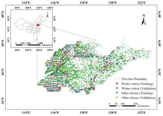
2.1. Study Area
2.2. Data and Preprocessing
2.2.1. Remote Sensing Data
2.2.2. Sample Data Acquisition
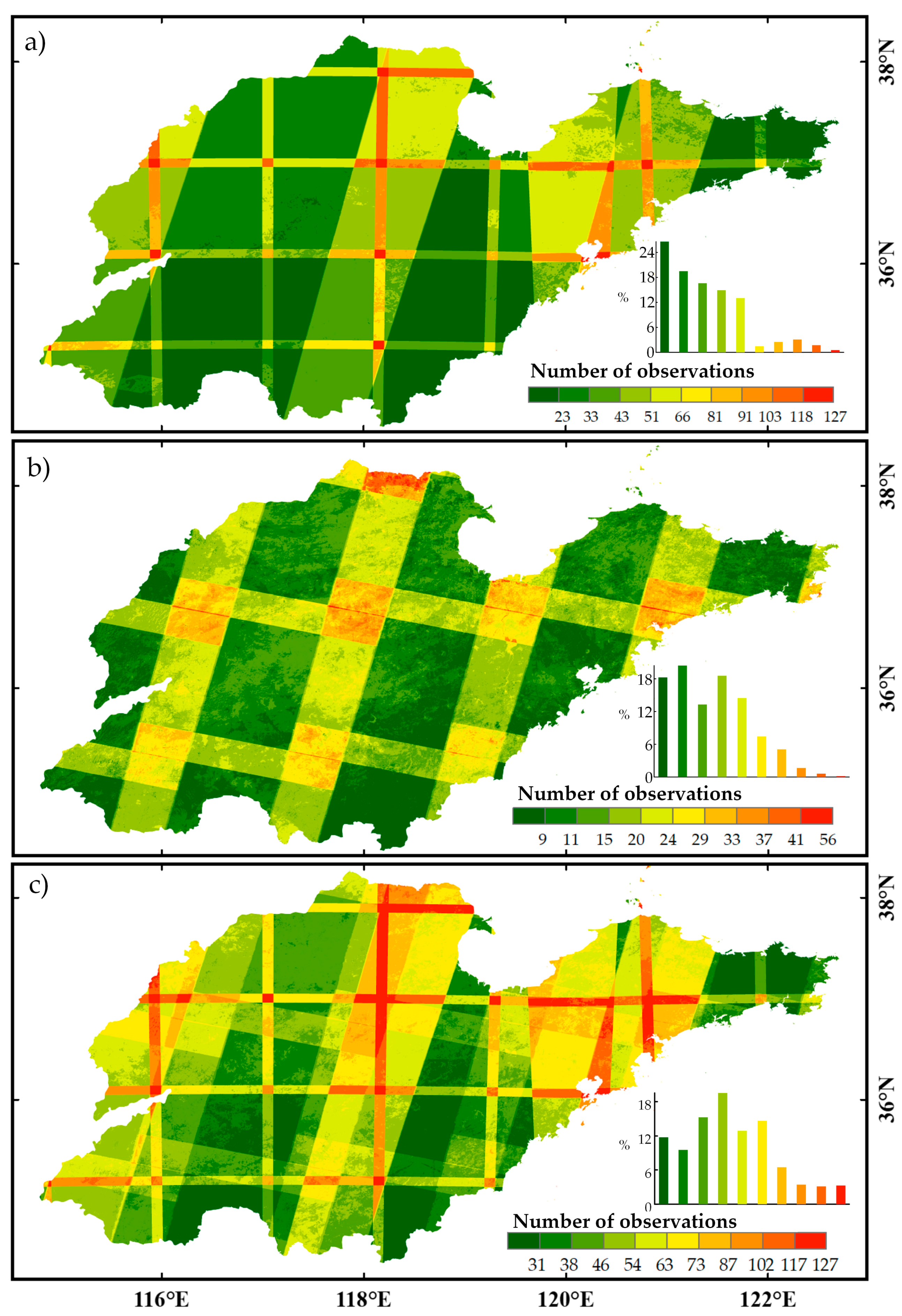
3. Methodology
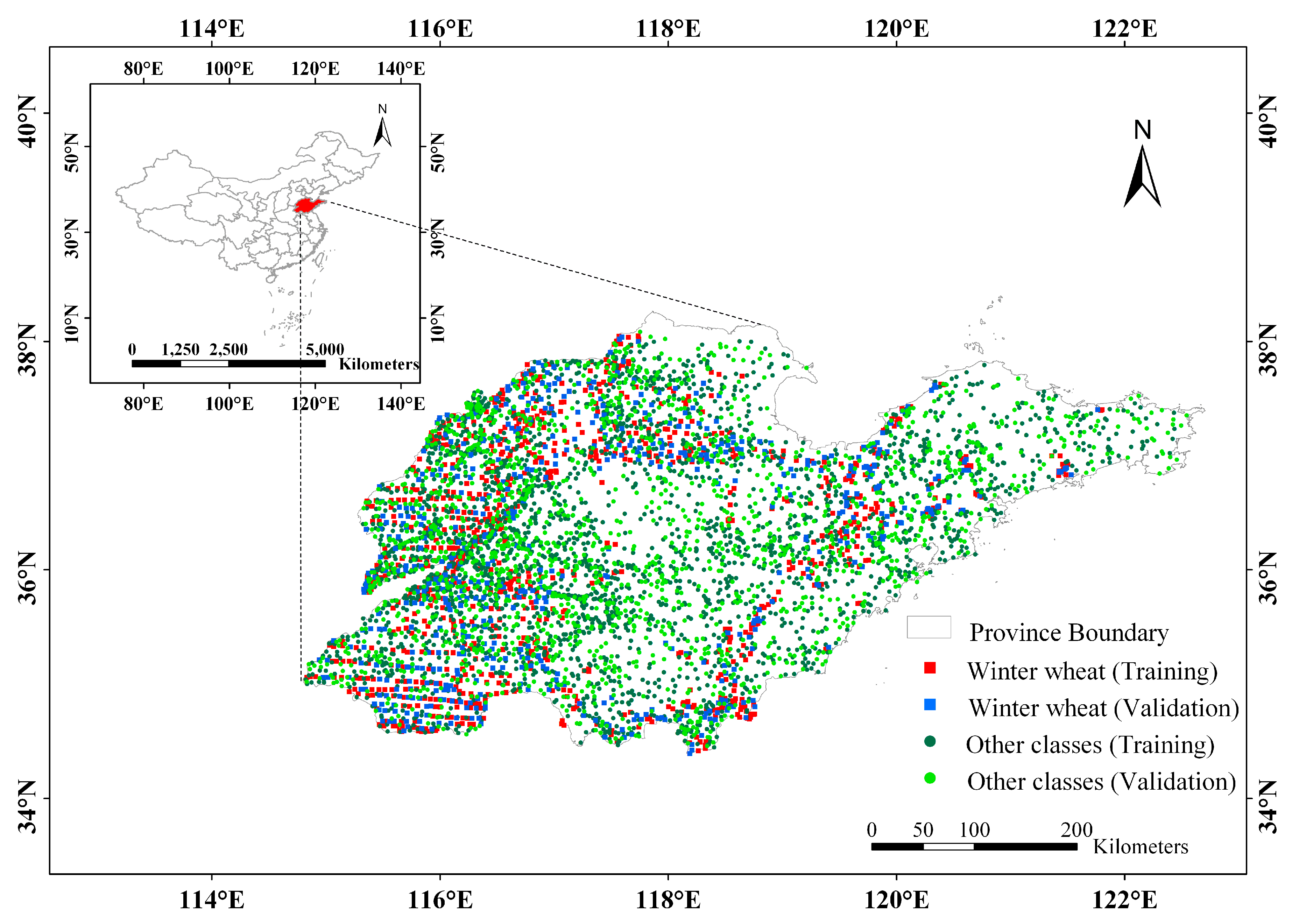
3.1. Temporal Aggregation
3.2. Feature Calculation
3.3. Random Forest Classifier
3.4. Accuracy Assessment
3.5. Feature Importance Assessment
4. Results
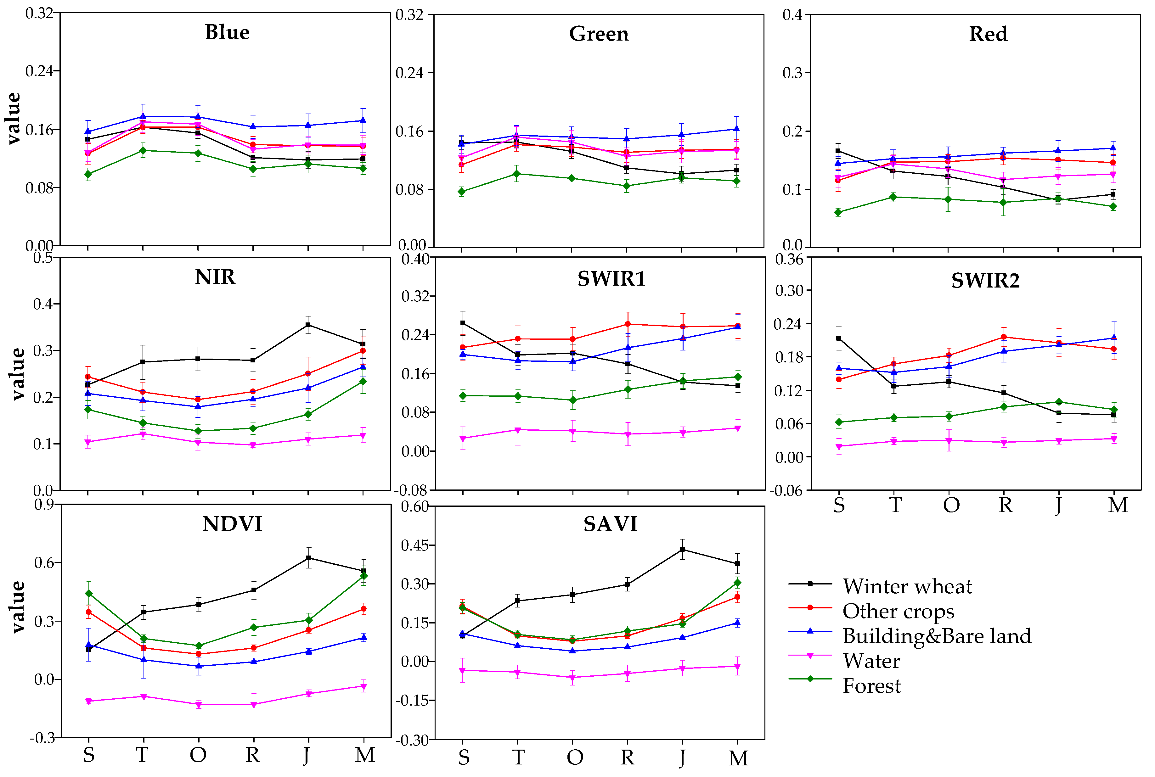
4.1. Spectral Differences of Features
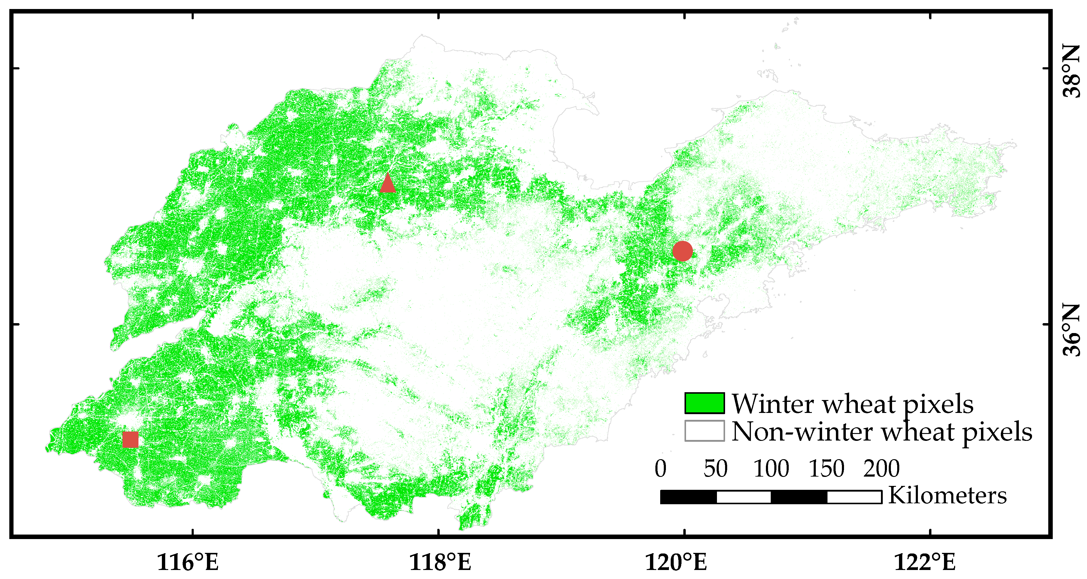
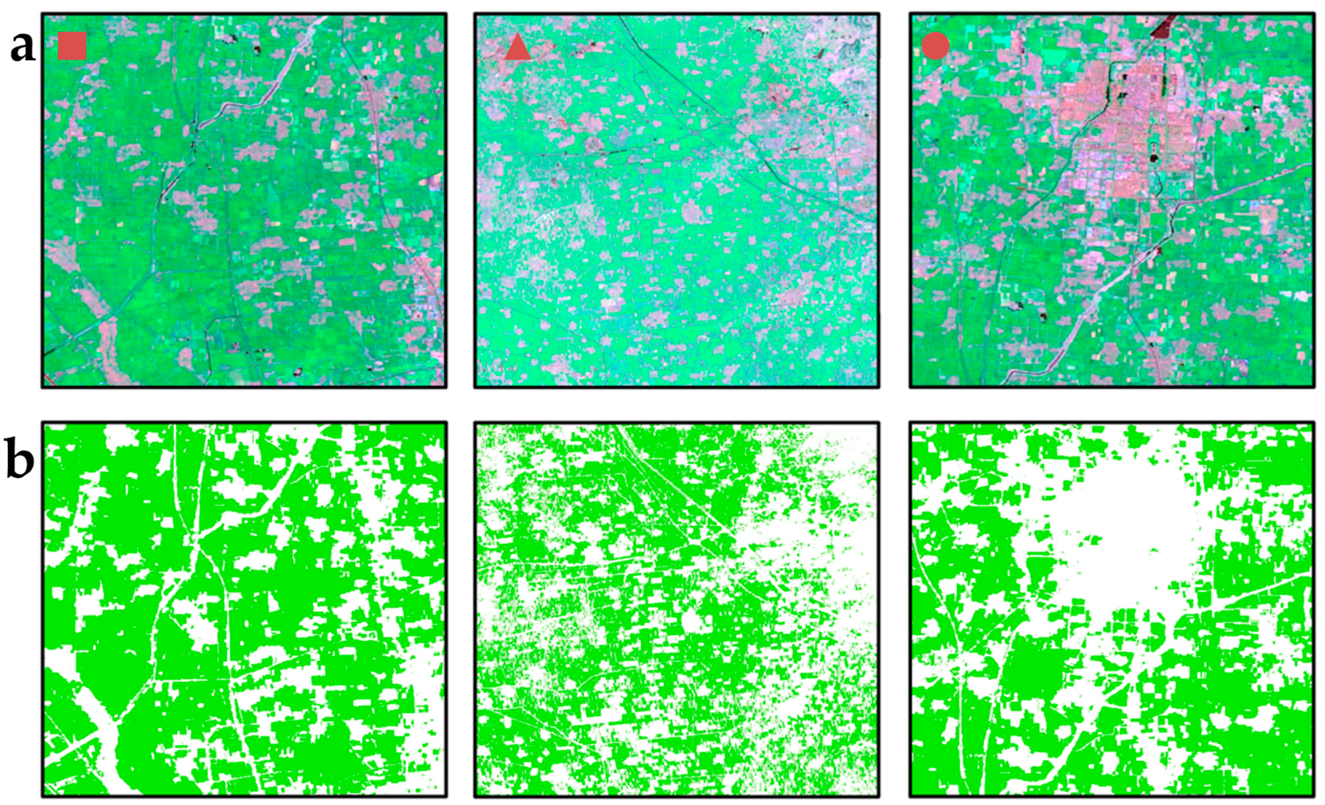
4.2. Winter Wheat Map in Shandong
4.3. Comparison with Mono-Temporal Data
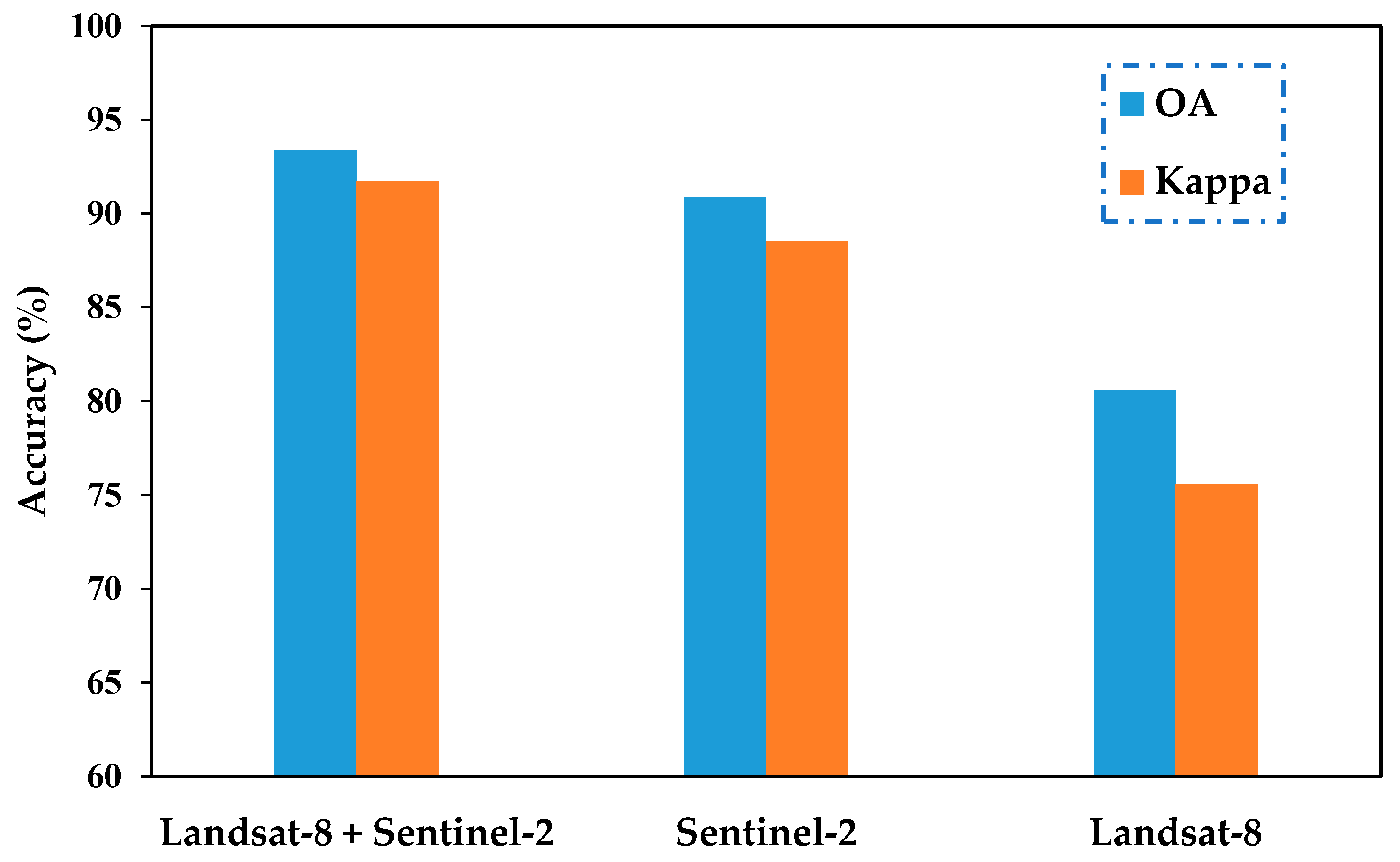
4.4. Comparison with Single Sensors’ Data
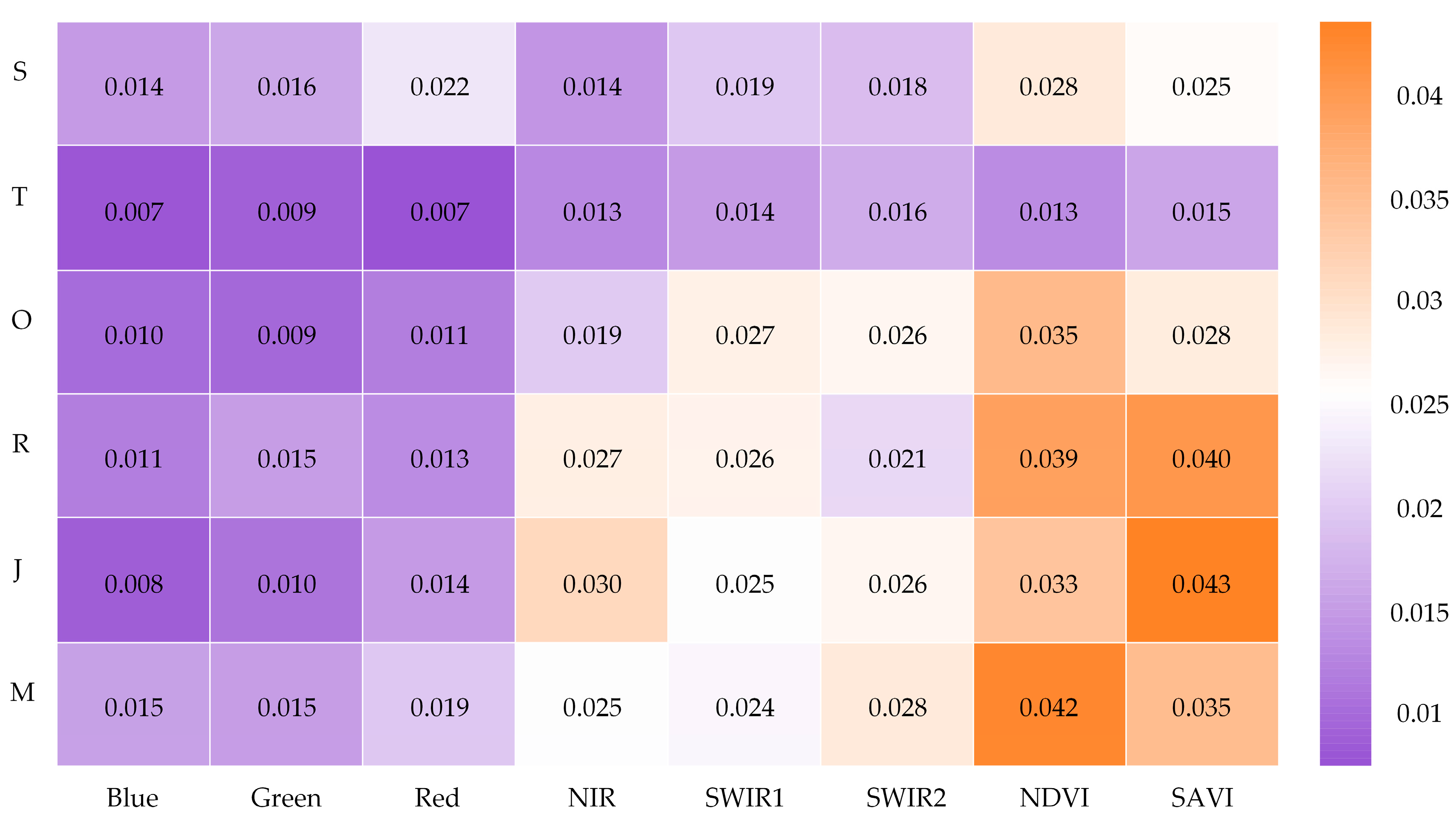
4.5. Feature Importance
5. Discussion
5.1. Combining of Temporally Aggregated Landsat-8 and Sentinel-2 Data
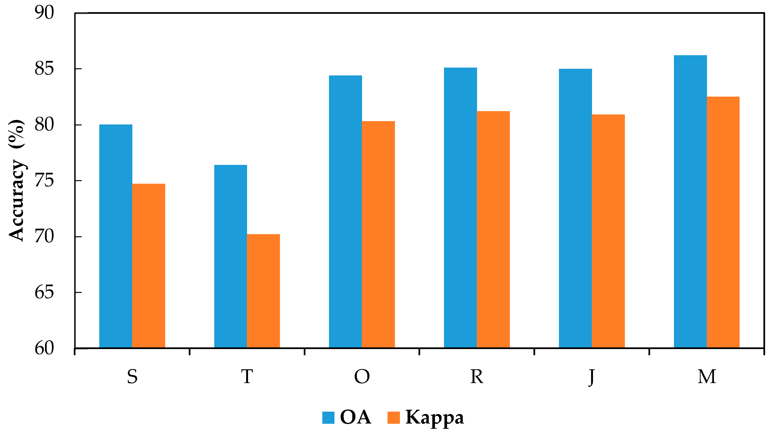
5.2. The Impact of Key Crop Development Phases on Classification Results
5.3. Uncertainty and Outlook
6. Conclusions
Supplementary Materials
Author Contributions
Funding
Acknowledgments
Conflicts of Interest
References
- Food and Agriculture Organization of the United Nations. FAOSTAT Statistics Database, Food Balance Sheets. Available online: www.fao.org/faostat/en/#data/FBS (accessed on 12 September 2019).
- Food and Agriculture Organization of the United Nations, FAOSTAT Statistics Database, Crops. Available online: www.fao.org/faostat/en/#data/QC (accessed on 12 September 2019).
- Qiu, B.; Luo, Y.; Tang, Z.; Chen, C.; Lu, D.; Huang, H.; Chen, Y.; Chen, N.; Xu, W. Winter wheat mapping combining variations before and after estimated heading dates. Isprs J. Photogramm. 2017, 123, 35–46. [Google Scholar] [CrossRef]
- Friedl, M.A.; Sulla-Menashe, D.; Tan, B.; Schneider, A.; Ramankutty, N.; Sibley, A.; Huang, X. MODIS Collection 5 global land cover: Algorithm refinements and characterization of new datasets. Remote Sens. Environ. 2010, 114, 168–182. [Google Scholar] [CrossRef]
- Gong, P.; Wang, J.; Yu, L.; Zhao, Y.; Zhao, Y.; Liang, L.; Niu, Z.; Huang, X.; Fu, H.; Liu, S.; et al. Finer resolution observation and monitoring of global land cover: First mapping results with Landsat TM and ETM+ data. Int. J. Remote Sens. 2013, 34, 2607–2654. [Google Scholar] [CrossRef]
- Yang, L.; Jin, S.; Danielson, P.; Homer, C.; Gass, L.; Bender, S.M.; Case, A.; Costello, C.; Dewitz, J.; Fry, J.; et al. A new generation of the United States National Land Cover Database: Requirements, research priorities, design, and implementation strategies. Isprs J. Photogramm. 2018, 146, 108–123. [Google Scholar] [CrossRef]
- Dong, J.; Xiao, X.; Menarguez, M.A.; Zhang, G.; Qin, Y.; Thau, D.; Biradar, C.; Moore, B. Mapping paddy rice planting area in northeastern Asia with Landsat 8 images, phenology-based algorithm and Google Earth Engine. Remote Sens. Environ. 2016, 185, 142–154. [Google Scholar] [CrossRef] [PubMed]
- He, Y.; Wang, C.; Chen, F.; Jia, H.; Liang, D.; Yang, A. Feature Comparison and Optimization for 30-M Winter Wheat Mapping Based on Landsat-8 and Sentinel-2 Data Using Random Forest Algorithm. Remote Sens. 2019, 11, 535. [Google Scholar] [CrossRef]
- Dong, J.; Xiao, X.; Kou, W.; Qin, Y.; Zhang, G.; Li, L.; Jin, C.; Zhou, Y.; Wang, J.; Biradar, C.; et al. Tracking the dynamics of paddy rice planting area in 1986–2010 through time series Landsat images and phenology-based algorithms. Remote Sens. Environ. 2015, 160, 99–113. [Google Scholar] [CrossRef]
- Zhang, M.; Lin, H. Object-based rice mapping using time-series and phenological data. Adv. Space Res. 2019, 63, 190–202. [Google Scholar] [CrossRef]
- He, T.; Xie, C.; Liu, Q.; Guan, S.; Liu, G. Evaluation and Comparison of Random Forest and A-LSTM Networks for Large-scale Winter Wheat Identification. Remote Sens. 2019, 11, 1665. [Google Scholar] [CrossRef]
- Yang, Y.; Tao, B.; Ren, W.; Zourarakis, D.P.; Masri, B.E.; Sun, Z.; Tian, Q. An Improved Approach Considering Intraclass Variability for Mapping Winter Wheat Using Multitemporal MODIS EVI Images. Remote Sens. 2019, 11, 1191. [Google Scholar] [CrossRef]
- Tao, J.; Wu, W.; Zhou, Y.; Wang, Y.; Jiang, Y. Mapping winter wheat using phenological feature of peak before winter on the North China Plain based on time-series MODIS data. J. Integr. Agric. 2017, 16, 348–359. [Google Scholar] [CrossRef]
- Pan, Y.; Li, L.; Zhang, J.; Liang, S.; Zhu, X.; Sulla-Menashe, D. Winter wheat area estimation from MODIS-EVI time series data using the Crop Proportion Phenology Index. Remote Sens. Environ. 2012, 119, 232–242. [Google Scholar] [CrossRef]
- Liu, J.; Feng, Q.; Gong, J.; Zhou, J.; Liang, J.; Li, Y. Winter wheat mapping using a random forest classifier combined with multi-temporal and multi-sensor data. Int. J. Digit. Earth 2018, 11, 783–802. [Google Scholar] [CrossRef]
- Hao, P.; Wang, L.; Niu, Z. Potential of multitemporal Gaofen-1 panchromatic/multispectral images for crop classification: Case study in Xinjiang Uygur Autonomous Region, China. J. Appl. Remote Sens. 2015, 9. [Google Scholar] [CrossRef]
- Sun, C.; Bian, Y.; Zhou, T.; Pan, J. Using of Multi-Source and Multi-Temporal Remote Sensing Data Improves Crop-Type Mapping in the Subtropical Agriculture Region. Sensors 2019, 19, 2401. [Google Scholar] [CrossRef] [PubMed]
- PaxLenney, M.; Woodcock, C.E. Monitoring Agricultural Lands in Egypt with Multi-temporal Landsat TM Imagery: How Many Images Are Needed? Remote Sens. Environ. 1997, 59, 522–529. [Google Scholar] [CrossRef]
- Prishchepov, A.V.; Radeloff, V.C.; Dubinin, M.; Alcantara, C. The Effect of Landsat ETM/ETM+ Image Acquisition Dates on the Detection of Agricultural Land Abandonment in Eastern Europe. Remote Sens. Environ. 2012, 126, 195–209. [Google Scholar] [CrossRef]
- Alcantara, C.; Kuemmerle, T.; Prishchepov, A.V.; Radeloff, V.C. Mapping abandoned agriculture with multi-temporal MODIS satellite data. Remote Sens. Environ. 2012, 124, 334–347. [Google Scholar] [CrossRef]
- Oetter, D.R.; Cohen, W.B.; Berterretche, M.; Maiersperger, T.K.; Kennedy, R.E. Land cover mapping in an agricultural setting using multiseasonal Thematic Mapper data. Remote Sens. Environ. 2001, 76, 139–155. [Google Scholar] [CrossRef]
- Roy, D.P.; Wulder, M.A.; Loveland, T.R.; Woodcock, C.E.; Allen, R.G.; Anderson, M.C.; Scambos, T.A. Landsat-8: Science and Product Vision for Terrestrial Global Change Research. Remote Sens. Environ. 2014, 145, 154–172. [Google Scholar] [CrossRef]
- Wulder, M.A.; White, J.C.; Loveland, T.R.; Woodcock, C.E.; Belward, A.S.; Cohen, W.B.; Roy, D.P. The global Landsat archive: Status, consolidation, and direction. Remote Sens. Environ. 2016, 185, 271–283. [Google Scholar] [CrossRef]
- Park, S.; Im, J.; Park, S.; Yoo, C.; Han, H.; Rhee, J. Classification and Mapping of Paddy Rice by Combining Landsat and SAR Time Series Data. Remote Sens. 2018, 10, 447. [Google Scholar] [CrossRef]
- Singha, M.; Dong, J.; Zhang, G.; Xiao, X. High resolution paddy rice maps in cloud-prone Bangladesh and Northeast India using Sentinel-1 data. Sci. Data. 2019, 6. [Google Scholar] [CrossRef] [PubMed]
- Zhong, L.; Hu, L.; Zhou, H. Deep learning based multi-temporal crop classification. Remote Sens. Environ. 2019, 221, 430–443. [Google Scholar] [CrossRef]
- Li, J.; Roy, D.P. A Global Analysis of Sentinel-2A, Sentinel-2B and Landsat-8 Data Revisit Intervals and Implications for Terrestrial Monitoring. Remote Sens. 2017, 9, 902. [Google Scholar]
- Zhang, X.; Qiu, F.; Qin, F. Identification and mapping of winter wheat by integrating temporal change information and Kullback-Leibler divergence. Int. J. Appl. Earth Obs. 2019, 76, 26–39. [Google Scholar] [CrossRef]
- Xiong, J.; Thenkabail, P.S.; Tilton, J.C.; Gumma, M.K.; Teluguntla, P.; Oliphant, A.; Congalton, R.G.; Yadav, K.; Gorelick, N. Nominal 30-m Cropland Extent Map of Continental Africa by Integrating Pixel-Based and Object-Based Algorithms Using Sentinel-2 and Landsat-8 Data on Google Earth Engine. Remote Sens. 2017, 9, 1065. [Google Scholar] [CrossRef]
- Carrasco, L.O.; Neil, A.; Morton, R.; Rowland, C. Evaluating Combinations of Temporally Aggregated Sentinel-1, Sentinel-2 and Landsat 8 for Land Cover Mapping with Google Earth Engine. Remote Sens. 2019, 11, 288. [Google Scholar] [CrossRef]
- Löw, F.; Prishchepov, A.V.; Waldner, F.; Dubovyk, O.; Akramkhanov, A.; Biradar, C.; Lamers, J. Mapping Cropland Abandonment in the Aral Sea Basin with MODIS Time Series. Remote Sens. 2018, 10, 159. [Google Scholar] [CrossRef]
- Zhang, X.; Wu, B.; Ponce-Campos, G.; Zhang, M.; Chang, S.; Tian, F. Mapping up-to-Date Paddy Rice Extent at 10 M Resolution in China through the Integration of Optical and Synthetic Aperture Radar Images. Remote Sens. 2018, 10, 1200. [Google Scholar] [CrossRef]
- Tian, F.; Wu, B.; Zeng, H.; Zhang, X.; Xu, J. Efficient Identification of Corn Cultivation Area with Multitemporal Synthetic Aperture Radar and Optical Images in the Google Earth Engine Cloud Platform. Remote Sens. 2019, 11, 629. [Google Scholar] [CrossRef]
- Gorelick, N.; Hancher, M.; Dixon, M.; Ilyushchenko, S.; Thau, D.; Moore, R. Google Earth Engine: Planetary-Scale Geospatial Analysis for Everyone. Remote Sens. Environ. 2017, 202, 18–27. [Google Scholar] [CrossRef]
- Hansen, M.C.; Potapov, P.V.; Moore, R.; Hancher, M.; Turubanova, S.A.; Tyukavina, A.; Kommareddy, A. High-Resolution Global Maps of 21st-Century Forest Cover Change. Science 2013, 342, 850–853. [Google Scholar] [CrossRef] [PubMed]
- Zhang, W.; Brandt, M.; Wang, Q.; Prishchepov, A.V.; Tucker, C.J.; Li, Y.; Lyu, H.; Fensholt, R. From woody cover to woody canopies: How Sentinel-1 and Sentinel-2 data advance the mapping of woody plants in savannas. Remote Sens. Environ. 2019, 234, 111465. [Google Scholar] [CrossRef]
- National Census Data of China. Available online: http://data.stats.gov.cn/ (accessed on 12 September 2019).
- Zhu, Z.; Woodcock, C.E. Object-based cloud and cloud shadow detection in Landsat imagery. Remote Sens. Environ. 2012, 118, 83–94. [Google Scholar] [CrossRef]
- Tucker, C.J. Red and photographic infrared linear combinations for monitoring vegetation. Remote Sens. Environ. 1979, 8, 127–150. [Google Scholar] [CrossRef]
- Huete, A.R.; Hua, G.; Qi, J.; Chehbouni, A.; Van Leeuwen, W.J.D. Normalization of multidirectional red and NIR reflectances with the SAVI. Remote Sens. Environ. 1992, 41, 143–154. [Google Scholar] [CrossRef]
- Feng, Q.; Gong, J.; Liu, J.; Li, Y. Monitoring Cropland Dynamics of the Yellow River Delta based on Multi-Temporal Landsat Imagery over 1986 to 2015. Sustainability 2015, 7, 14834–14858. [Google Scholar] [CrossRef]
- Jin, Z.; Azzari, G.; You, C.; Di Tommaso, S.; Aston, S.; Burke, M.; Lobell, D.B. Smallholder maize area and yield mapping at national scales with Google Earth Engine. Remote Sens. Environ. 2019, 228, 115–128. [Google Scholar] [CrossRef]
- Zurqani, H.A.; Post, C.J.; Mikhailova, E.A.; Schlautman, M.A.; Sharp, J.L. Geospatial analysis of land use change in the Savannah River Basin using Google Earth Engine. Int. J. Appl. Earth Obs. 2018, 69, 175–185. [Google Scholar] [CrossRef]
- Rodriguez-Galiano, V.F.; Ghimire, B.; Rogan, J.; Chica-Olmo, M.; Rigol-Sanchez, J.P. An assessment of the effectiveness of a random forest classifier for land-cover classification. Isprs J. Photogramm. 2012, 67, 93–104. [Google Scholar] [CrossRef]
- Zhong, L.; Gong, P.; Biging, G.S. Efficient corn and soybean mapping with temporal extendability: A multi-year experiment using Landsat imagery. Remote Sens. Environ. 2014, 140, 1–13. [Google Scholar] [CrossRef]
- Pelletier, C.; Valero, S.; Inglada, J.; Champion, N.; Dedieu, G. Assessing the robustness of Random Forests to map land cover with high resolution satellite image time series over large areas. Remote Sens. Environ. 2016, 187, 156–168. [Google Scholar] [CrossRef]
- Congalton, R.G. A review of assessing the accuracy of classifications of remotely sensed data. Remote Sens. Environ. 1991, 37, 35–46. [Google Scholar] [CrossRef]
- Schuster, C.; Schmidt, T.; Conrad, C.; Kleinschmit, B.; Forster, M. Grassland habitat mapping by intra-annual time series analysis—Comparison of RapidEye and TerraSAR-X satellite data. Int. J. Appl. Earth Obs. Geoinf. 2015, 34, 25–34. [Google Scholar] [CrossRef]
- Pedregosa, F.; Varoquaux, G.; Gramfort, A.; Michel, V.; Thirion, B.; Grisel, O.; Blondel, M.; Prettenhofer, P.; Weiss, R.; Dubourg, V.; et al. Scikit-learn: Machine Learning in Python. J. Mach. Learn. Res. 2011, 12, 2825–2830. [Google Scholar]
- Yang, X.; Lo, C.P. Using a time series of satellite imagery to detect land use and land cover changes in the Atlanta, Georgia metropolitan area. Int. J. Remote Sens. 2002, 23, 1775–1798. [Google Scholar] [CrossRef]
- Storey, J.; Roy, D.P.; Masek, J.; Gascon, F.; Dwyer, J.; Choate, M. A note on the temporary misregistration of Landsat-8 Operational Land Imager (OLI) and Sentinel-2 Multi Spectral Instrument (MSI) imagery. Remote Sens. Environ. 2016, 186, 121–122. [Google Scholar] [CrossRef]
- Van der Werff, H.; van der Meer, F. Sentinel-2A MSI and Landsat 8 OLI Provide Data Continuity for Geological Remote Sensing. Remote Sens. 2016, 8, 883. [Google Scholar] [CrossRef]


| Month | Oct | Nov | Dec | Jan | Feb | Mar | Apr | May | Jun | ||||||||||||||||||
|---|---|---|---|---|---|---|---|---|---|---|---|---|---|---|---|---|---|---|---|---|---|---|---|---|---|---|---|
| Ten-day | I | II | III | I | II | III | I | II | III | I | II | III | I | II | III | I | II | III | I | II | III | I | II | III | I | II | III |
| Winter wheat | |||||||||||||||||||||||||||
| Satellite Platform | Landsat-8 | Sentinel-2 |
|---|---|---|
| Sensor | OLI | MSI |
| Image extent | 170 × 185 km | 100 × 100 km |
| Spatial resolution utilized bands | 30 m | 10/20 m |
| Repeat cycle | 16 days | 5 days |
| Utilized bands | Band2 (Blue: 0.49–0.51 μm) | Band 2 (Blue: 0.46–0.52 μm) |
| Band 3 (Green: 0.53–0.59 μm) | Band 3 (Green: 0.54–0.58 μm) | |
| Band 4 (Red: 0.64–0.67 μm) | Band 4 (Red: 0.65–0.69 μm) | |
| Band 5 (NIR: 0.85–0.88 μm) | Band 8A (NIR: 0.86–0.89 μm) | |
| Band 6 (SWIR1: 1.57–1.65 μm) | Band 11 (SWIR1: 1.57–1.66 μm) | |
| Band 7 (SWIR2: 2.11–2.29 μm) | Band 12 (SWIR2: 2.10–2.29 μm) |
| Class | Training Pixels | Validation Pixels |
|---|---|---|
| Winter wheat | 907 | 605 |
| Other crops | 660 | 440 |
| Building and bare land | 871 | 580 |
| Water | 787 | 525 |
| Forest | 486 | 324 |
| Data | Crop Development Phase | Image Acquisition Period | Number of Sentinel-2 MSI Images | Number of Landsat-8 OLI Images | Total Number of Images |
|---|---|---|---|---|---|
| Landsat-8 + Sentinel-2 | Seeding | 1, Oct–31, Oct | 323 | 38 | 361 |
| Tillering | 1, Nov–10, Dec | 255 | 46 | 301 | |
| Over-wintering | 11, Dec–20, Feb | 464 | 72 | 536 | |
| Reviving | 21, Feb–31, Mar | 240 | 44 | 284 | |
| Jointing-Heading | 1, Apr–30, Apr | 230 | 32 | 262 | |
| Maturing | 1, May–10, Jun | 301 | 44 | 345 | |
| Sentinel-2 | Seedling–Tillering | 1, Oct–10, Dec | 578 | 0 | 578 |
| Over-wintering–Reviving | 11, Dec–31, Mar | 704 | 0 | 704 | |
| Jointing-Heading | 1, Apr–30, Apr | 230 | 0 | 230 | |
| Maturing | 1, May–10, Jun | 301 | 0 | 301 | |
| Landsat-8 | Entire growing period | 1, Oct–10, Jun | 0 | 276 | 276 |
| Classification | Validation Samples | Sum | UA | F1 | ||||
|---|---|---|---|---|---|---|---|---|
| Winter Wheat | Other Crops | Building and Bare Land | Water | Forest | ||||
| Winter wheat | 595 | 20 | 4 | 0 | 1 | 620 | 98.3% | 0.97 |
| Other crops | 6 | 353 | 15 | 7 | 20 | 401 | 80.2% | 0.84 |
| Building and bare land | 1 | 24 | 551 | 2 | 2 | 580 | 95% | 0.94 |
| Water | 1 | 2 | 4 | 515 | 4 | 526 | 98.1% | 0.98 |
| Forest | 2 | 41 | 6 | 1 | 297 | 347 | 91.7% | 0.89 |
| Sum | 605 | 440 | 580 | 525 | 324 | 2474 | OA= 93.4% | Kappa = 91.7% |
| PA | 96% | 88% | 95% | 97.9% | 85.6% | |||
© 2020 by the authors. Licensee MDPI, Basel, Switzerland. This article is an open access article distributed under the terms and conditions of the Creative Commons Attribution (CC BY) license (http://creativecommons.org/licenses/by/4.0/).
Share and Cite
Xu, F.; Li, Z.; Zhang, S.; Huang, N.; Quan, Z.; Zhang, W.; Liu, X.; Jiang, X.; Pan, J.; Prishchepov, A.V. Mapping Winter Wheat with Combinations of Temporally Aggregated Sentinel-2 and Landsat-8 Data in Shandong Province, China. Remote Sens. 2020, 12, 2065. https://doi.org/10.3390/rs12122065
Xu F, Li Z, Zhang S, Huang N, Quan Z, Zhang W, Liu X, Jiang X, Pan J, Prishchepov AV. Mapping Winter Wheat with Combinations of Temporally Aggregated Sentinel-2 and Landsat-8 Data in Shandong Province, China. Remote Sensing. 2020; 12(12):2065. https://doi.org/10.3390/rs12122065
Chicago/Turabian StyleXu, Feng, Zhaofu Li, Shuyu Zhang, Naitao Huang, Zongyao Quan, Wenmin Zhang, Xiaojun Liu, Xiaosan Jiang, Jianjun Pan, and Alexander V. Prishchepov. 2020. "Mapping Winter Wheat with Combinations of Temporally Aggregated Sentinel-2 and Landsat-8 Data in Shandong Province, China" Remote Sensing 12, no. 12: 2065. https://doi.org/10.3390/rs12122065
APA StyleXu, F., Li, Z., Zhang, S., Huang, N., Quan, Z., Zhang, W., Liu, X., Jiang, X., Pan, J., & Prishchepov, A. V. (2020). Mapping Winter Wheat with Combinations of Temporally Aggregated Sentinel-2 and Landsat-8 Data in Shandong Province, China. Remote Sensing, 12(12), 2065. https://doi.org/10.3390/rs12122065