Forest Potential Productivity Mapping by Linking Remote-Sensing-Derived Metrics to Site Variables

Abstract

A fine-resolution region-wide map of forest site productivity is an essential need for effective large-scale forestry planning and management. In this study, we incorporated Sentinel-2 satellite data into an increment-based measure of forest productivity (biomass growth index (BGI)) derived from climate, lithology, soils, and topographic metrics to map improved BGI (iBGI) in parts of North American Acadian regions. Initially, several Sentinel-2 variables including nine single spectral bands and 12 spectral vegetation indices (SVIs) were used in combination with forest management variables to predict tree volume/ha and height using Random Forest. The results showed a 10–12 % increase in out of bag (OOB) r² when Sentinel-2 variables were included in the prediction of both volume and height together with BGI. Later, selected Sentinel-2 variables were used for biomass growth prediction in Maine, USA and New Brunswick, Canada using data from 7738 provincial permanent sample plots. The Sentinel-2 red-edge position (S2REP) index was identified as the most important variable over others to have known influence on site productivity. While a slight improvement in the iBGI accuracy occurred compared to the base BGI model (~2%), substantial changes to coefficients of other variables were evident and some site variables became less important when S2REP was included.

1. Introduction

Forest productivity is an important measurement for sustainable forest planning and management and carbon sequestration studies and can be estimated from gross primary productivity (GPP) or potential site quality. While GPP is the ecological measure of productivity that estimates the total amount of organic matter fixed through photosynthesis, site productivity estimates the potential of a particular forest stand to produce aboveground wood and is usually quantified as a site index (SI). Methods based on SI are the most common and widely used measures of forest productivity, but these methods are often site-specific and species-dependent, leading to bias in the comparison of productivity in different regions [1]. In addition, SI estimation in regions dominated by multi-cohort and mixed-species can be challenging. In these regions, a variety of other approaches can be used to determine and quantify potential site productivity [2].

Fine-resolution, region-wide mapping of forest productivity is desired for improved comparison of productivity among and within regions as well as large-scale planning and management, particularly with respect to evaluating the effect of climate change on ecosystems. However, these maps are generally not available for many regions yet. Several attempts have been made to map potential forest productivity at regional scale [3,4,5]. However, updated regional productivity maps across different climatic regions will be more desired for a wide range of disciplines. The production of these maps can be done through process-based models, remote sensing techniques and the merger of both approaches [4,5].

Several studies have related the observed SI to climate variables [1] and soil [6], or modeled potential productivity using process-based ecosystem models [4,7], which allow potential productivity to be mapped across different regions. Remote sensing techniques have been applied more to estimate GPP mainly using two approaches: i) employing remotely sensed indices as proxies for GPP [8,9,10] and ii) using remote sensing variables as inputs for GPP models [11,12,13,14,15,16,17]. Through the concept of linear relationship between SI and leaf area index (LAI) [18], a model was suggested to map SI at 1 km spatial resolution using the MODIS enhanced vegetation index (EVI) for Douglas-fir (Pseudotsuga menziesii (Mirb.) Franco) across the Pacific and Inland Northwest, USA [5]. Optical multispectral data such as Landsat imagery have been used to estimate forest structural attributes such as height, volume, and biomass [19,20,21], which have been previously identified as the best forest productivity indicators [22].

Recently, a fine-resolution region-wide map of forest productivity called the biomass growth index (BGI) was suggested for the quantification of forest site potential productivity for Acadian regions of the USA and Canada [2]. This model is an increment-based index that is a better alternative to SI in forests with complex stand types. Past management practices and naturally-induced disturbances have transformed the transitional Acadian Region into a region with more complex stand structures and species composition, needing alternative methods to account for these key trends in future modeling.

BGI is defined as the maximum stand above-ground biomass net growth rate (kg ha⁻¹ year⁻¹) and is estimated using climatic, lithology, soil, and topographic variables. It offers several advantages over SI as it is a better model for mixed and multi-cohort forests like those in northeastern USA including the state of Maine, has a fine spatial resolution (20 m) and is independent of past management, unlike SI. BGI is also a quantitative, species-independent, and unified site productivity model suitable for use in forests having complex structures, such as those in the Acadian Forest Region of North America. Nonetheless, in its current form, the model explains only approximately 50% of the variation in plot above-ground biomass growth, and is limited by poor soils data resolution, high underlying variability between species, and an incomplete stand development history not fully considered in the model [2]. Knowing that SI can be modeled using remote sensing data [5,23], there is a strong potential for the improvement of the BGI model by the additional incorporation of remotely sensed variables.

In general, limited studies are available that link higher resolution remote sensing imagery with site variables to map potential productivity for regions with multiple tree species. Recently, field inventory, Landsat spectral bands, and ecological variables were used to produce SI and mean annual increment (MAI) maps at 30 m spatial resolution for the Tahoe National Forest (TNF), California, USA [3]. New developments in satellite remote sensing technology have offered greater possibilities for additional improvement of current methodologies. The European Sentinel-2 mission includes the Sentinel-2A and -2B satellites launched in June 2015 and March 2017, respectively. Data from these satellites are free-of-charge and preliminary products are currently available globally. With newly launched Sentinel-2 satellites, we have access to finer spectral (13 spectral bands), temporal (less than five days), and spatial (10–20 m) resolution data compared with Landsat imagery that has a 30 m spatial and 16 days temporal resolutions.

Several spectral vegetation indices (SVIs), such as the normalized difference vegetation index (NDVI) and EVI, have been suggested to estimate forest biophysical variables such as LAI and productivity [24]. Landsat spectral bands have been used for the estimation of forest structural attributes such as height, volume, and biomass [20,21]. Sentinel-2 imagery has spectral bands in the red-edge region that were not available in multi-spectral satellites like Landsat. These spectral bands are more efficient for the quantification of forest biophysical attributes such as leaf chlorophyll content, LAI and fractional vegetation cover [25,26,27], which could be potentially helpful to improve potential forest productivity estimation and have yet to be fully investigated to our knowledge.

This research aimed at employing several remotely sensed variables obtained from Sentinel-2 satellite data to produce an improved BGI model. The specific objectives of this research were: (1) assessing the potential capabilities of several Sentinel-2-derived SVIs and single spectral bands for forest productivity measurement through evaluating the Sentinel-2 variables to predict tree volume and height; (2) using the best Sentinel-2 variables in combination with site variables for modeling and mapping forest potential productivity across New Brunswick, Canada and Maine, USA at 20 m spatial resolution; (3) comparing the improved BGI using remote sensing variables to the original BGI to better understand regional differences and areas of future improvement.

2. Materials and Methods

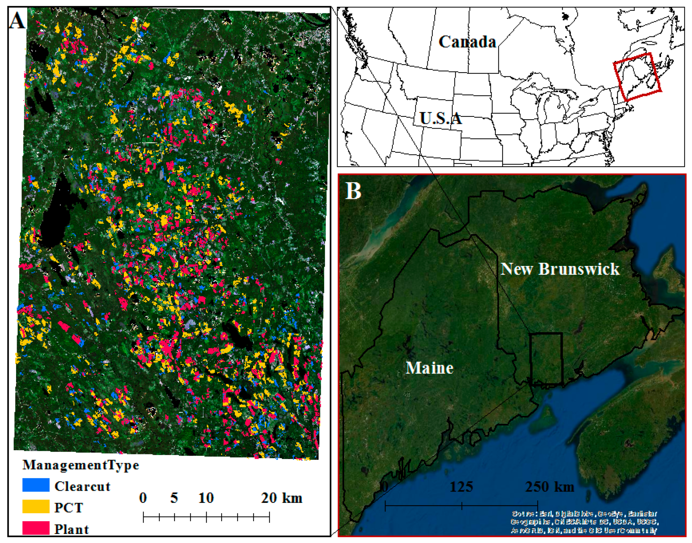
The overall methodology of this study is shown in Figure 1. All components of the workflow are explained in the following sections.

2.1. Study Area

The study area covers parts of the Acadian forest region of the United States and Canada. The Acadian forest region is a transitional zone between two larger forest ecosystems, the northern broadleaf forest to the south and the boreal forest to the north, and encompasses three Canadian Maritime Provinces (New Brunswick, Nova Scotia, and Prince Edward Island), parts of southern Quebec, as well as northern New England states including Maine. Two major predominant forest types are spruce-fir forests comprising in particular red spruce (Picea rubens Sarg.) and balsam fir (Abies balsamea (L.) Mill.), and the northern hardwood forest, where sugar maple (Acer saccharum Marsh.), American beech (Fagus grandifolia Ehrh.), and yellow birch (Betula alleghaniensis Britton) are dominant. Other common tree species are red maple (Acer rubrum L.), eastern hemlock (Tsuga canadensis (L.) Carr.), eastern white pine (Pinus strobus L.), and northern white-cedar (Thuja occidentalis L.) [28]. The Acadian forest has been greatly altered by a long history of human-induced changes such as land clearing, intensive timber harvesting, and silvicultural practices, as well as natural disturbances, windstorms and insect outbreak in particular. Therefore, the majority of the Acadian forest is dominated by naturally-regenerated, mixed-species stands having either even- or uneven-aged structures. Two study area extents were used in this study. Figure 2A shows the extent of the study area in New Brunswick, Canada where several Sentinel-2 variables were evaluated and selected for forest productivity modeling, and Figure 2B shows the extent of the study area where a potential forest productivity map was produced using the suggested model.

2.2. Field Data

For the study area in New Brunswick (Figure 2A), different sets of field data were collected. In particular, New Brunswick Crown Lands’ forest management polygon data [29], which contained photo-interpreted species composition, treatment history, and year of treatment, were used. This information allowed us to determine species percentages, stand age and management type (Mgmt) (i.e., planted, pre-commercial thinning (PCT), clearcut regeneration). BGI data [2] and Light Detection and Ranging (LiDAR)-derived forest inventory predictions, both having 20 m spatial resolution, were also collected [30].

To map forest potential productivity for Maine and New Brunswick (Figure 2B), a total of 7033 existing forest inventory plots, measured by government and industrial forestry organizations across Maine and New Brunswick, were used in this study. These included: (1) New Brunswick Department of Natural Resources and Energy Development (NB-DNRED) provincial permanent sample plots for tree growth research; (2) Acadian Timber Inc. permanent sample plots in northwestern New Brunswick; (3) Maine state continuous forest inventory plots from the Forest Inventory and Analysis Unit, USDA Forest Service.

Biomass growth of surviving trees (BG; kg ha⁻¹ year⁻¹) for all the plots were provided through [2]. BG_pm was calculated using aboveground dry biomass of all trees in a plot (p) that are alive at the start of a plot measurement period (m) between two measurement periods as explained in [2]. Plot measurements prior to 1990 were excluded from the analysis to avoid the possible effects of the 1970–1980s spruce budworm (Choristoneura fumiferana Clem.) outbreak on growth estimates. Pre-commercially thinned and planted stands also were excluded and tree ages between 20 and 100 years were used [2].

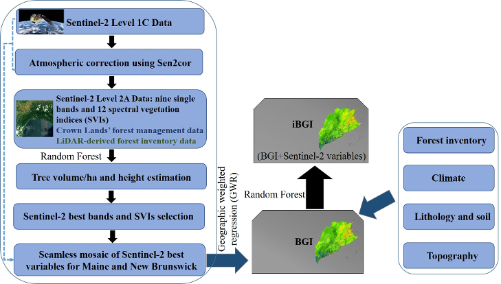
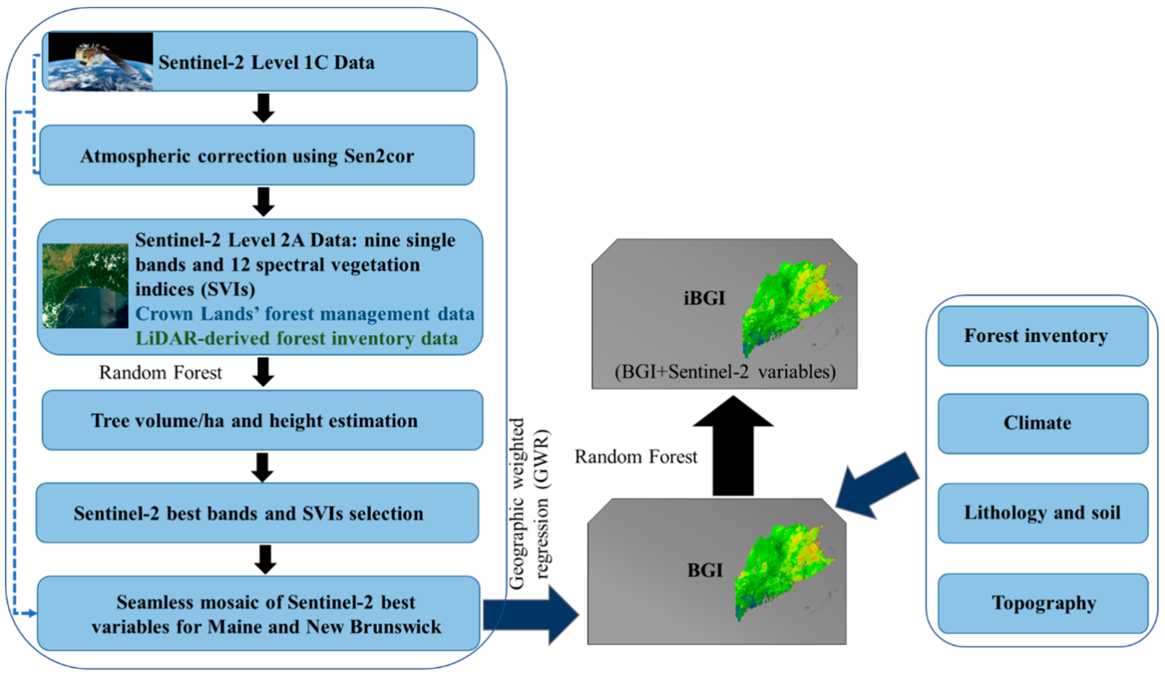
2.3. Remote Sensing Data Collection and Processing

Sentinel-2 A and B Level 1C Top-Of-Atmosphere (L1C-TOA) reflectance products during summer time were collected for this study. For the first part of the study, two cloud-free Sentinel-2 A L1C-TOA images, dated July 31 and September 14, 2017, were collected for our study site, located in the southern parts of New Brunswick, from https://earthexplorer.usgs.gov/ (Figure 2A). No cloud-free imagery was available for the month of August. The Sentinel-2 SNAP toolbox and the Sen2Cor processor were used for atmospheric-, terrain and cirrus cloud corrections of L1C-TOA products. The L1C-TOA imagery were converted to L2A surface reflectance products. Then, several SVIs were computed from Sentinel-2 spectral bands using L2A products at 20 m resolution. The list of SVIs and their equations along with single spectral bands (total of 21 Sentinel-2 satellite derived variables) used in this study is presented in

Table 1. Sentinel-2 variables used in the study (all at 20 m spatial resolution).

No	Band/Index *	Band info/ /Formulation	Reference
1	b2	Blue (490 nm)	-----------
2	b3	Green (560 nm)
3	b4	Red (665 nm)
4	b5	Vegetation Red-Edge (705 nm)
5	b6	Vegetation Red-Edge (740 nm)
6	b7	Vegetation Red-Edge (783 nm)
7	b8a	Near Infrared (NIR) (865 nm)
8	b11	Shortwave Infrared (1610 nm)
9	b12	Shortwave Infrared (2190 nm)
10	CLre	(b7/b5) − 1	[31]
11	EVI7	2.5× (b7 − b4)/(b7 + 6 × b4 − 7.5 × b2 + 1)	[32]
12	EVI8	2.5× (b8a − b4)/(b8a + 6 × b4 − 7.5 × b2 + 1)	[33]
13	GNDVI	(b7 − b3)/(b7 + b3)	[34]
14	IRECI	(b7 − b4)/(b5/b6)	[35]
15	NDVI	(b8a − b4)/(b8a + b4)	[36]
16	NDVI45	(b5 − b4)/(b5 + b4)	[25]
17	NDVI65	(b6 − b5)/(b6 + b5)	[37]
18	MSR	((b7/b4) − 1)/((b7/b4) + 1) 0.5	[38]
19	MTCI	(b6 − b5)/(b5− b4)	[39]
20	S2REP	705 + 35 × ((b4 + b7)/2 − b5)/(b6 − b5)	[40]
21	WDRVI	(0.01 × b7 − b5)/(0.01 × b7 + b5)+(1 − 0.01)/(1 + 0.01)	[32]

* CLre: Red-edge Chlorophyll Index; EVI7: Enhanced Vegetation Index using b5; EVI8a: Enhanced Vegetation Index using b8a; GNDVI: Greenness Normalized Difference Vegetation Index; IRECI: Inverted red-edge chlorophyll index; NDVI: Normalized Difference Vegetation Index using b4 and b8a; NDVI45: NDVI using b4 and b5; NDVI65: NDVI using b6 and b5; MSR: Modified Simple Ratio; MTCI: MERIS terrestrial chlorophyll; S2REP: Sentinel-2 red-edge position; WDRVI: Wide Dynamic Range Vegetation Index.

.

The initial selection of SVIs and band combinations was based on their performance in previous studies to measure vegetation biochemical and biophysical properties such as chlorophyll content, leaf area index (LAI), biomass and volume using Sentinel-2 or other multi- or hyperspectral sensors [27,32,41,42,43]. The red-edge region (spectral range between 690 and 730 nm) is suggested to be more effective for the measurement of vegetation biophysical and biochemical parameters and, in contrast to red (centered at 670 nm) and green (centered at 550 nm) reflectance, has been found to be more sensitive to a wide range of chlorophyll content. For this reason, SVIs derived from red-edge bands are expected to be a better measure for chlorophyll content, LAI, biomass, and tree volume compared with traditional SVIs [26,44,45]. Therefore, in this study several red-edge SVIs were evaluated (Table 1). We used Sentinel-2-derived variables for the prediction of the total bole inside-bark volume (TV) and height of the thickest 100 trees per hectare (HT; i.e. top height) as a proxy of forest productivity [22].

In the second part of the study, which mapped forest potential productivity over the entire study region (Figure 2B), 58 Sentinel-2A and B L1C-TOA images dated between July 20 and September 14 in both 2017 and 2018 were collected from https://earthexplorer.usgs.gov/ to create a seamless mosaic of the best Sentinel-2-derived variables selected from the first part of the study for Maine and New Brunswick. Similarly, as described above, the Sentinel-2 SNAP toolbox was used to convert the LIC-TOA imagery to L2A surface reflectance products.

2.4. Prediction of Total Bole Inside-bark Volume (TV) and Height of Thickest 100 Trees (HT)

LiDAR-derived predictions of TV and HT on a 20 × 20 m point feature grid, acquired from the NB-DNRED, were intersected with the 21 Sentinel-2 variables (nine spectral bands and 12 vegetation indices) from two different dates (July 31 and September 14, 2017). The resulting 20×20 m point layer was intersected again with the New Brunswick crown forest management polygon layer, which contained photo-interpreted species composition, treatment history, as well as year of treatment, and allowed us to determine species percentages, stand age and management type (i.e., planted, PCT and clearcut regeneration) for each point. Sentinel-2-derived variables, in combination with other variables such as photo-interpreted species composition of stands, stand age and management history, and BGI, were used to predict LiDAR-derived TV and HT in our study site in New Brunswick (Figure 2A). In this case, we used TV and HT as if they were measured directly, rather than modeled responses. In New Brunswick, TV and especially HT were predicted at high accuracy from LiDAR point clouds with r² of 0.7–0.8 and 0.8–0.9, respectively [30]. TV and HT were modeled using Random Forests (RF) [46] using stand species composition, stand age, stand management type, BGI, and Sentinel-2 spectral bands and indices. Only stands that were > 1 acre were used in RF models (7400 stands total) [46]. With LiDAR HT and stand age, site index can be calculated. Here we were interested in identifying whether Sentinel-2 variables explain additional variability in point and stand-level LiDAR-TV and -HT beyond what could already be predicted by age, species, management type, and BGI. Bands that showed good predictive power and low auto-correlation could be carried forward to improve the BGI model.

2.5. Site Factors

Site factors (variables) used in this research are the same variables used in [2] to model the base BGI, including climate, lithology, soils, and topography variables. Monthly climate normals (1971–2000) at 800 m resolution were acquired from [47]. Lithology and soil data were obtained from various sources (

Table 2. Site variables used in the study.

Variables		Resolution	Reference/Data Provider
Climate	Mean growing season temperature normals 1971–2000 Frost-free days normals 1971–2000	800 m	[47]
Lithology and soil	Bedrock productivity index (BRI) derived from rock type observed regional effect on site Root growing space index (RGS) derived as a combination of maximum root depth and percent course fragment	resampled to 50 m	[2]
Topography	Depth to water (DTW) predicted at 10 m resolution from DEM Slope in degrees	20 m	[48]

) and resampled to 50 m. A variety a topographic variables were estimated based on existing digital elevation models (DEMs) and resampled to 20 m. Topographical variables consisted of elevation, depth to water (DTW) [48], slope (°), and System for Automated Geoscientific Analyses (SAGA) terrain indices [49] such as topographic wetness, roughness, positive openness, and slope position class.

2.6. Using Sentinel-2 Variables to Improve BGI in Maine and New Brunswick

BG responses to site factors and the best Sentinel-2-derived variables selected from the first part of the study were explored using the nonparametric RF regression tree algorithm [46]. Before using Sentinel-2-derived variables for modeling forest potential productivity, the following procedure was applied to the imagery to normalize and smooth the data.

We noted significant observable differences between Sentinel-2 values captured in July compared to late August and early September. While preference was given to late summer captures, large cloud-free captures in Maine and New Brunswick were unavailable in late summer in certain areas, and for those areas, normalized July images were used. Normalization was performed by linearly regressing late summer imagery against July imagery where spatially coincident for undisturbed forested areas, and then predicting late summer values from the July values where needed.

We used an adaptation of a geographic weighted regression (GWR) technique to develop smoothed Sentinel-2 best variable mosaics for New Brunswick and Maine separately as a function of elevation, slope, and log depth to water + 0.0001 on a 20 m grid by: (1) sampling Sentinel-2 variables, elevation, slope, and depth to water attributes on a 250 m grid; (2) omitting sample points that were: (a) non-forest or wetland, recently harvested (since 1990) based on Landsat-based disturbance history data (up to 2010 for Maine using Forest Disturbance History from Landsat, 1986–2010 [50] and up to 2015 for New Brunswick using Landsat harvest and fire change history products from 1985–2015 [51], (b) recent disturbances identified with Sentinel-2 b3 > 0.06, and (c) areas missing Sentinel-2 coverage (no cloud free days ~ 5% of total area); (3) using least squares to solve approximately 1.5 million liner models, one for each grid-point (966,728 for Maine, 687,876 for New Brunswick), using the closest 30 grid-point attributes as local samples and stepwise backward variable selection using a significance-level < 0.05 as a threshold for variable inclusion, and where no variables were significant, the average observed Sentinel-2 variable value was used for that model; (4) predicting local distance-weighted average Sentinel-2 variables using the closest 30 linear models for each point location on a 20 m grid for the entire New Brunswick and Maine areas.

We trained this model by varying the number of point observations (10–200) used to build each model, and the number of models (10–200) used to predict the Sentinel-2 optimal variables at each grid point, and chose numbers that, on average, minimized predicted Sentinel-2 variable RMSE using ten-fold cross validation. Smoothed Sentinel-2 variables slightly outperformed unsmoothed variables in terms of Random Forest variable importance (always ranked higher), therefore smoothed data were used exclusively for all further analyses. Smoothed variables were added to the original BGI model as an additional asymptotic term and model coefficients were then re-solved for New Brunswick and Maine plots, together.

2.7. Adding Sentinel-2 Terms to Biomass Growth Non-Linear Equation

Smoothed Sentinel-2 variables found useful for predicting biomass growth were introduced as additive asymptotic terms in the original Chapman–Richards biomass growth equation (BG) [2] with the base and new models were refit using only Maine and New Brunswick (Nova Scotia and Prince Edward Island excluded). The revised BG equation (iBG) and refit coefficients were used to map the new Sentinel-2-informed BGI, herein called ‘iBGI’, throughout New Brunswick and Maine. The two equations were then compared and areas of interest were determined for further exploration.

3. Results

3.1. Prediction of TV and HT using Field and Sentinel-2 Variables

A 10–12 % increase in out of bag (OOB) r² was observed when Sentinel-2 variables were included in the prediction of TV (

Table 3. Results of total volume (m³/ha) (TV) prediction by Random Forest using species composition, age, management type, BGI and Sentinel-2 spectral bands and indices.

Response	Predictor Variables	OOB r2	RMSE
Total volume/ha (TV)	Age, Species, Mgmt., BGI	68.8%	24.5
	Age, Species, Mgmt., BGI, July Sentinel-2 (all variables)	80.5%	19.3
	Age, Species, Mgmt., BGI, September Sentinel-2 (all variables)	79.9%	19.7
	Age, Mgmt., BGI, July Sentinel-2 (all variables)	78.7%	20.2
	Age, Mgmt., BGI, July Sentinel-2 (b3, b8a, b11, S2REP, NDVI45)	78.5%	20.3
	Age, Mgmt., BGI, July Sentinel-2 (b3, b8a, S2REP)	77.2%	20.9
	All July Sentinel-2 bands and indices	66.1%	25.5
	July Sentinel-2 (b3, b8a, S2REP)	57.9%	28.4

). The prediction of stand-level TV based on age, species composition, Mgmt, and BGI yielded an OOB r² of 68.8%, whereas the addition of the July and September Sentinel-2 data increased the OOB r² to 80.5%. Additionally, dropping species composition as a predictor variable did not significantly affect the OOB r² (79.9% vs. 78.7%). After reviewing the construction of the correlation matrix of the bands and indices, we dropped all bands and indices with the exception of bands b3, b8a, and b11 and indices S2REP and NDVI45, yielding no change in model results (OOB r²: 78.7% to 78.5%). Partial dependence plots showed a strong relationship between volume and b3, b8a, and S2REP, but a relatively poor relationship with band b11 and NDVI45. Random Forest models using age, Mgmt, BGI, and only b3, b8a, and S2REP resulted in a slight reduction in OOB r² (78.5% vs. 77.2%). Dropping age and Mgmt and running the model on only BGI, b3, b8a, and S2REP yielded an OOB r² of 61.2% and, finally, using only Sentinel-2 best variables (b3, b8a, S2REP) resulted in an OOB r² of around 58%. Results for TV prediction using September Sentinel-2 data were similar to July results where adding September variables in combination with age, species composition, Mgmt, and BGI increased the OOB r² from 68.8% to 79.9% (Table 3).

Results for HT prediction incorporating Sentinal-2 data were similar to those obtained for TV and are presented in

Table 4. Results of height (HT) (m) prediction by Random Forest using species composition, age, management type, BGI and Sentinel-2 spectral bands and indices.

Response	Predictor Variables	OOB r2	RMSE
Height (HT)	Age, Species, Mgmt., BGI	59.7%	1.6
	Age, Species, Mgmt., BGI, July Sentinel-2 (all variables)	70.3%	1.3
	Age, Species, Mgmt., BGI, September Sentinel-2 (all variables)	70.1%	1.3
	Age, Mgmt., BGI, July Sentinel-2 (all variables)	67.4%	1.4
	Age, Mgmt., BGI, July Sentinel-2 (b3, b8a, b11, S2REP, NDVI45)	66.8%	1.4
	Age, Mgmt., BGI, July Sentinel-2 (b3, b8a, S2REP)	64.7%	1.5
	All July Sentinel-2 bands and indices	56.8%	1.6
	July Sentinel-2 (b3, b8a, S2REP)	45.0%	1.8

. Incorporating Sentinel-2 variables increased predication accuracy by 10% (OOB r² from 59.7% to 70.3%). Based on the performance of Sentinel-2 variables to predict TV and HT, two single spectral bands (b3 and b8a) and one SVI (S2REP) were selected to be used for modeling forest potential productivity at landscape scale.

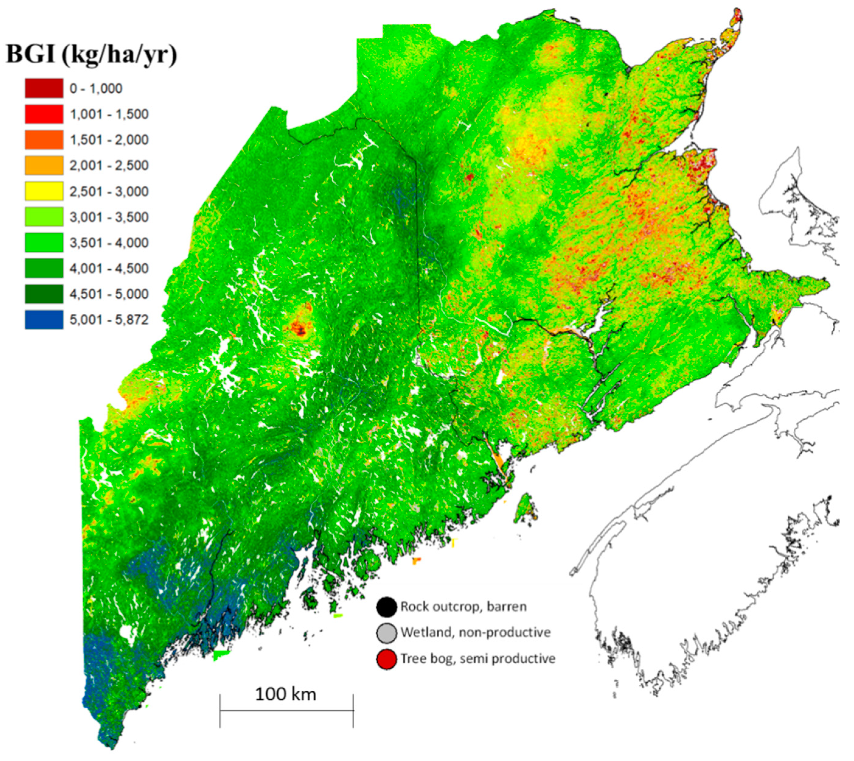
3.2. Improving Biomass Growth Index Model for Maine and New Brunswick

Before incorporating two Sentinel-2 single spectral bands and SVIs to model forest potential productivity, the correlations between the extracted variables were evaluated using 7038 forest inventory plots in Maine and New Brunswick. The results showed that NIR (b8a) reflectance and S2REP were not strongly correlated (r~0.2). However, green reflectance (b3) was correlated with S2REP and b8a (r~0.5). Moreover, b8a and S2REP more strongly correlated with plot biomass growth rate (r~0.25–0.30), but green band were not correlated with plot biomass growth rate. Due to the low performance of b3 to predict plot biomass growth rate and total biomass, only NIR (b8a) and S2REP were used for the addition to the model. The list of the variables used for model selection and the final model is presented in

Table 5. List of the site and Sentinel-2 variables used for model development.

Variable	Used in the Final Model	Description (also See [2])
BM	Yes	Biomass > 9 cm DBH in trees that survive to the next measurement period
HW	No	% hardwood composition by basal area
QMD9	Yes	Quadratic mean diameter (cm) > 9 cm DBH
S2REP_GWR	Yes	S2REP smoothed with GWR
Ffree	Yes	Frost-free days
AvgTempGS	Yes	Average growing season temperature
BRI	Yes	Bed rock fertility index
PO	Yes	% Poplar spp. basal area
Slope	Yes	% Slope
b8a	No	NIR (no smoothing)
Pi	Yes	% Pine basal area
DWT	Yes	Depth to water table
RGS	Yes	Root growing space (0–100 cm)

DBH: diameter at breast height, GWR: geographic weighted regression.

.

The performances of the three variable combinations are presented in

Table 6. Improved biomass growth index (iBGI; kg ha⁻¹ year⁻¹) model performance using Random Forest (RF) as compared with the base biomass growth index (BGI) model.

Model Fit Statistics
Base Model		Base Model +S2REP		Base Model + S2REP + b8a		Base Model + S2REP + b8a+ HW
n	7738	n	7738	n	7738	n	7738
MB	1.08	MB	3.95	MB	2.59	MB	2.80
MAB	673.62	MAB	663.01	MAB	657.80	MAB	653.42
RMSE	862.62	RMSE	852.10	RMSE	845.60	RMSE	840.70
r2	46.6%	r2	47.9%	r2	48.7%	r2	49.3%
Influential variables
Variable	% MSE Incr.	Variable	% MSE Incr.	Variable	% MSE Incr.	Variable	% MSE Incr.
BM	63.49%	BM	54.93%	BM	58.89%	BM	59.16%
Ffree	10.77%	S2REP_GWR	10.59%	b8a	9.11%	HW	11.63%
PO	8.44%	QMD9	7.61%	QMD9	8.24%	QMD9	9.40%
BRI	8.39%	AvgTempGS	7.59%	S2REP_GWR	7.21%	S2REP_GWR	5.97%
QMD9	8.16%	PO	7.25%	Ffree	6.95%	Ffree	5.31%
AvgTempGS	7.16%	Ffree	6.92%	PO	5.64%	AvgTempGS	4.97%
Slope	6.87%	BRI	5.49%	AvgTempGS	5.15%	BRI	4.66%
DWT	4.51%	Slope	4.88%	BRI	5.08%	PO	3.98%
RGS	1.78%	DWT	2.50%	Slope	3.37%	Slope	3.40%
Pi	1.04%	RGS	1.92%	RGS	1.54%	b8a	3.20%
		Pi	0.66%	DWT	1.45%	Pi	1.85%
				Pi	1.02%	DWT	1.54%
						RGS	0.95%

n: number of plots, MB: mean bias, MAB: mean absolute bias, RMSE: root mean square error, % MSE Incr.: percent increase in mean square error (MSE) if the variable is removed from the model.

. When S2REP was added to site variables to predict BG, it resulted in an r² of 47.9%. Adding NIR (b8a) and % hardwood composition by basal area (HW) variables slightly increased the performance of the model to 48.7% and 49.3%, respectively. S2REP was highly significant as an asymptote term in the BGI model and outperformed all site variables when it was added to the model. While only a slight improvement in accuracy occurred, substantial changes to coefficients of other variables were evident; i.e., some variables became less important when S2REP was included. When NIR and S2REP were added to the model, r² increased slightly but NIR showed a high correlation with hardwood content (HW) (Table 6) and therefore was removed from the final model.

Finally, only S2REP was selected for the inclusion in the model used for mapping the improved forest potential productivity index (improved BGI; iBGI). The base model, the new model and their components are presented in Equations (1)–(7).

$$B{G}_{pm}=(CLIMAT{E}_p+SOI{L}_p+TOPOGRAPH{Y}_p+SPECIE{S}_{pm})\times {\left(1-e^{-b_{0}B{M}_{pm}/1000}\right)}^{c_0+c_{1}QM{D}_{PM}}$$

(1)

$$iB{G}_{pm}=(CLIMAT{E}_p+SOI{L}_p+TOPOGRAPH{Y}_p+SPECIE{S}_{pm}+SENTINEL{2}_{pm})\times {\left(1-e^{-b_{0}B{M}_{pm}/1000}\right)}^{c_0+c_{1}QM{D}_{PM}}$$

(2)

$$CLIMATE=a_0+a_1\times Ffre{e}_p+a_2\times AvgTempG{S}_p$$

(3)

$$SOIL=a_3\times \ln \left(RG{S}_p+10\right)+a_4\times BR{I}_p$$

(4)

$$TOPOGRAPHY=a_5\times \ln \left(DW{T}_p+0.0001\right)+a_6\times \left(SLOP{E}_p^{s_0}\times e^{-s_{1}SLOP{E}_p}\right)$$

(5)

$$SPECIES=a_7\times P{O}_{pm}+a_8\times P{i}_{pm}$$

(6)

$$SENTINEL2=a_9\times S2REP\_GW{R}_p$$

(7)

where the asymptote of original BGI and new BGI (iBGI) were defined by a combination of site factors (CLIMATE, SOIL, TOPOGRAPHY; see Table 2), SPECIES (percent basal area of PO and Pi) and SENTINEL-2 (S2REP_GWR) factors with parameters a₀, …,a₉, s₀, and s₁; the growth rate parameter b₀ was influenced by plot aboveground dry biomass (BM) at time 0 surviving to time 1; and the shape parameters c₀ and c₁ were influenced by the quadratic mean diameter (QMD) at time 0 (

Table 7. Biomass growth model variables and nonlinear model parameter estimates for Equations (1)–(7).

Variable (Parameter)	Base BGI Model				iBGI Model				% Change
	Coeff.	SE	T	p-Value	Coeff.	SE	T	p-Value
Intercept (a0)	−4573	445	−10.278	0.000	−272,737	13201	−20.661	0.000	-
Ffree (a1)	18.71	1.28	14.612	0.000	14.75	1.21	12.240	0.000	79%
AveTempGS (a2)	273.13	35.54	7.684	0.000	392.59	34.96	11.230	0.000	144%
DCFI (a3)	296.41	38.39	7.721	0.000	245.70	36.48	6.736	0.000	83%
BRFI (a4)	1234.1	72.25	17.082	0.000	921.52	67.80	13.593	0.000	75%
DWT(a5)	87.72	8.55	10.264	0.000	59.25	8.04	7.368	0.000	68%
Slope (a6)	729.58	150.30	4.854	0.000	636.70	134.62	4.730	0.000	87%
Slope (s0)	0.76	0.17	4.435	0.000	0.78	0.19	4.111	0.000	103%
Slope (s1)	0.16	0.04	4.237	0.000	0.18	0.05	3.946	0.000	110%
PO (a7)	18.18	1.07	16.988	0.000	9.05	1.02	8.838	0.000	50%
Pi (a8)	7.56	1.06	7.123	0.000	16.86	1.02	16.607	0.000	223%
Biomass (b0)	0.01	0.00	11.029	0.000	0.01	0.00	11.946	0.000	83%
QMD (c0)	−0.01	0.05	−0.244	0.807	−0.11	0.06	−1.839	0.066	846%
QMD (c1)	0.05	0.01	8.902	0.000	0.05	0.01	9.580	0.000	111%
S2REP (a9)	-	-	-	-	369.85	18.13	20.405	0.000	-

). All site variable values were bilinearly interpolated for each plot location (p), while stand variables, including BG, were calculated for each plot measurement period (m) [2]. To address heteroscedacity, a variance power function was included in the final model.

The map of base BGI for Maine and New Brunswick is presented in Figure 3. This map was produced based on Maine and New Brunswick permanent sample plots using coefficients presented in Table 7 and therefore can be slightly different from the BGI map presented in [2]. The asymptote of the iBG_pm model with species set at zero (iBGI) was also mapped at 20 m resolution for all of Maine and New Brunswick and is presented in Figure 4. The iBGI map was generally similar to the base BGI map (e.g., highest rates of productivity can be observed in the southern and central parts of Maine attributed to warmer growing conditions, deep soils, and fine sedimentary bedrocks). Lower productivity can be observed in highlands and coastal areas as well as poorly drained local topography, or areas with poor soils or bedrock.

The observed discrepancies between the iBGI and base BGI are related to two different factors: 1) on average, the BG model under-predicted the productivity in New Brunswick by about 235 kg ha⁻¹ year⁻¹ but over-predicted it in Maine by about 150 kg ha⁻¹ year⁻¹, and this difference was not much improved with the addition of S2REP to the iBG model. These differences can be attributed to variations related to the soil and lithology mapping procedures between regions (Maine and New Brunswick) that could not be fully standardized, and/or differences in regional species composition that could not be factored out of the BG model when mapping BGI and iBGI; 2) in general, low productivity (poor) sites, especially those with stocking limitations, in both Maine and New Brunswick are more detectable using Sentinel-2 data compared to high productivity sites; therefore, poor sites experienced the largest index change (reduction) when adding S2REP to the BG model for both regions. Therefore, the new iBGI map addressed the issues caused by rock, semi-barren land, or poor drainage. As an example, Figure 5 shows the new map clearly predicting poorer site productivity in areas of exposed rock in the New Brunswick highlands, when compared to the base BGI map, indicating an improvement.

4. Discussion

Sentinel-2-derived variables were used to predict LiDAR-estimated TV and HT, which were found to be quite effective either by themselves or used in combination with other ancillary data. Optical remote sensing data such as Landsat have been long used by numerous researchers to measure both forest biophysical and structural properties. While the application of SVIs is common for vegetation biophysical properties estimation [24], single spectral bands have commonly been used to measure structural properties [20,21] and productivity [3]. The application of Sentinel-2 data for estimating forest structural information and productivity is relatively new because they are recently-launched satellites. However, research has already shown the superiority of red-edge SVIs that can be calculated from Sentinel-2 data to measure vegetation biophysical variables [25,26,32,45,52].

In our research, two red-edge SVIs, namely S2REP and NDVI45, were identified as the best SVIs for TV and HT prediction among the 12 SVIs evaluated. The prediction of stand-level volume based on only Sentinel-2 variables was relatively promising (all variables OOB r²: 66%; only b3, b8a, S2REP variables OOB r²: 58%) and should be further tested across a broader range of conditions when more data becomes available. In our analysis, incorporating only Sentinel-2 variables with forest management data yielded an OOB r² > 80%. The prediction of HT based on only Sentinel-2 variables was also promising but the results were slightly lower than those for TV (all variables OOB r²: 56%; only b3, b8a, S2REP variables OOB r²: 45%). In contrast to TV, incorporating Sentinel-2 variables with forest management data yielded an OOB r² > 70%. Generally, optical remote sensing data provide more extensive information on forest structural attributes in the horizontal plane but are less effective to measure forest vertical structure, such as canopy height. Therefore, tree biophysical variables, such as LAI, crown size and tree diameter, have shown stronger correlation with optical variables compared to height [19,53].

S2REP was also strongly correlated with plot BG and in the new iBGI model, it was a highly significant variable and outperformed all other site variables when added to the BG model. However, NDVI45 did not have a strong relationship with plot BG and, therefore, was removed from further analysis. S2REP’s strong performance in productivity estimation is in agreement with previous studies that suggested this index as a robust index for LAI and chlorophyll content estimation [26]. To our knowledge, currently there is no literature available on S2REP performance for TV, HT and productivity estimation, but our findings imply a solid and rather encouraging relationship between this index and those parameters, which should be further assessed in future analyses.

Among single spectral bands, NIR (b8a) was identified as a significant variable to be used to estimate structural and biophysical parameters as well as productivity in previous research [3,20], however, as NIR showed high correlation with hardwood content, it was removed from our final model. Sentinel-2 b3 had a good performance to predict TV and HT but exhibited low performance to predict plot BG. This can be explained by the difference in forest maturity between modelled datasets in each analysis. The dataset used for the first part of the study to predict TV and HT was from younger stands but that used to model BGI/iBGI included mostly mature to old trees. However, b3 also was observed to be useful for identifying areas that were recently disturbed. For example, areas that were heavily disturbed (clearcut and roads) in the past 5–10 years nearly always had b3 reflectance values > 0.06. In addition, S2REP values commonly hovered around 716 to 726 for undisturbed productive forest land, but dropped sharply for areas recently disturbed, roads and agriculture. S2REP values were observed to remain lower than surrounding forest for 20–30 years post-harvest based on visual comparisons with Landsat-derived disturbance data from 1984–2015 in New Brunswick. It was visually apparent that, on average, S2REP values declined in areas with poor drainage and on semi-barren sites, and therefore seemed to be correlated to site productivity; however, within a given topographical position and local site, S2REP values were highly variable and probably influenced by other local factors than site, such as canopy gaps, canopy structure and species variation.

Although a slight improvement in the accuracy of the iBGI can be observed (around 2%), changes to coefficients of other site variables were substantial. S2REP was identified as the most important variable and was superior to climate, lithology, soils, and topographic site variables used to predict site productivity. Some soil and topography variables (e.g. RGS and DWT) became less important in the new model. Therefore, while climate variables [1], soil data [6] or a combination of site and climatic variables [2] are commonly used to map potential productivity across different regions, incorporating additional remote sensing data, particularly red-edge SVIs, seems to add an important new source of information for region-wide site productivity mapping. Although a model based on only remote sensing variables cannot explain all the variations in BG, these variables seem to have strong contributions and can potentially replace some of the site variables in the model. The productivity mapping incorporating remote sensing and site variables is promising but further improvements are still needed as our model performance and resulting maps highlight.

Several factors may have introduced errors or affected the performance of the new iBGI model and consequently, addressing these issues will potentially improve future model performance: (1) to produce a seamless mosaic of Sentinel-2 imagery, early summer imagery was employed for some tiles where mid-summer imagery was not available due to severe cloud cover; if those images are replaced by mid-summer images, the performance of the model will likely improve; (2) although several pre-processing steps were applied to produce cloud- and haze-free data for each tile in the mosaic, possible haze issues in 5 out of 26 tiles in each mosaic may still exist; a multi-date approach to produce composite images may address this issue; (3) the base BGI model was developed for Maine, New Brunswick, Nova Scotia, and Prince Edward Island and removing plots from Nova Scotia and Prince Edward Island resulted in less overall accuracy; (4) finally, obtaining higher positional accuracy of provincial permanent sample plot coordinates can improve the model’s overall performance.

5. Conclusions

The iBGI meets the criteria of a good site productivity measure as it incorporates both physical and biophysical characteristics of forest stands and it is species-independent, quantitative and comparable region wide. Seninel-2 satellite data provide useful spectral information and variables for estimating vegetation properties at fine spatial resolution and are a suitable source of information to measure tree structural components and forest site productivity. Among all Sentinel-2 variables, b3, b8a and S2REP were identified as the best variables for predicting TV and HT for young stands, while S2REP was identified as the best Sentinel-2 variable to predict biomass growth rate over all forest conditions.

These findings should help guide future efforts using Sentinel-2 data to predict forest structural attributes. Of particular interest in this region is using Sentinel-2 data to better map species composition and fine-scale, mixed-severity disturbances, which could also likely help to further improve BGI estimates. This, combined with the greater availability of regional LiDAR-derived forest metrics, should also provide better data needed to train and refine future maps of iBGI. Overall, the developed framework of combining remote sensing and site variables in this analysis showed promise and can be further applied in regions dominated by multi-cohort, mixed species forests.

References

1. Weiskittel, A.R.; Crookston, N.L.; Radtke, P.J. Linking climate, gross primary productivity, and site index across forests of the western United States. Can. J. For. Res. 2011, 41, 1710–1721. [Google Scholar] [CrossRef]
2. Hennigar, C.; Weiskittel, A.; Allen, H.L.; MacLean, D.A. Development and evaluation of a biomass increment based index for site productivity. Can. J. For. Res. 2017, 47, 400–410. [Google Scholar] [CrossRef] [Green Version]
3. Huang, S.; Ramirez, C.; Conway, S.; Kennedy, K.; Kohler, T.; Liu, J. Mapping site index and volume increment from forest inventory, Landsat, and ecological variables in Tahoe National Forest, California, USA. Can. J. For. Res. 2017, 47, 113–124. [Google Scholar] [CrossRef] [Green Version]
4. Swenson, J.J.; Waring, R.H.; Fan, W.; Coops, N. Predicting site index with a physiologically based growth model across Oregon, USA. Can. J. For. Res. 2005, 35, 1697–1707. [Google Scholar] [CrossRef] [Green Version]
5. Waring, R.H.; Milner, K.S.; Jolly, W.M.; Phillips, L.; McWethy, D. Assessment of site index and forest growth capacity across the Pacific and Inland Northwest USA with a MODIS satellite-derived vegetation index. For. Ecol. Manag. 2006, 228, 285–291. [Google Scholar] [CrossRef]
6. Jiang, H.; Radtke, P.J.; Weiskittel, A.R.; Coulston, J.W.; Guertin, P.J. Climate-and soil-based models of site productivity in eastern US tree species. Can. J. For. Res. 2015, 45, 325–342. [Google Scholar] [CrossRef]
7. Milner, K.S.; Running, S.W.; Coble, D.W. A biophysical soil–site model for estimating potential productivity of forested landscapes. Can. J. For. Res. 1996, 26, 1174–1186. [Google Scholar] [CrossRef]
8. Bunn, A.G.; Goetz, S.J. Trends in satellite-observed circumpolar photosynthetic activity from 1982 to 2003: The influence of seasonality, cover type, and vegetation density. Earth Interact. 2006, 10, 1–19. [Google Scholar] [CrossRef] [Green Version]
9. Goetz, S.J.; Bunn, A.G.; Fiske, G.J.; Houghton, R.A. Satellite-observed photosynthetic trends across boreal North America associated with climate and fire disturbance. Proc. Natl. Acad. Sci. USA 2005, 102, 13521–13525. [Google Scholar] [CrossRef] [Green Version]
10. Rossini, M.; Cogliati, S.; Meroni, M.; Migliavacca, M.; Galvagno, M.; Busetto, L.; Cremonese, E.; Julitta, T.; Siniscalco, M.C.; Morra di Cella, U. Remote sensing-based estimation of gross primary production in a subalpine grassland. Biogeosciences 2012, 9, 2565–2584. [Google Scholar] [CrossRef] [Green Version]
11. Joiner, J.; Yoshida, Y.; Zhang, Y.; Duveiller, G.; Jung, M.; Lyapustin, A.; Wang, Y.; Tucker, C.J. Estimation of terrestrial global gross primary production (GPP) with satellite data-driven models and eddy covariance flux data. Remote Sens. 2018, 10, 1346. [Google Scholar] [CrossRef] [Green Version]
12. Mahadevan, P.; Wofsy, S.C.; Matross, D.M.; Xiao, X.; Dunn, A.L.; Lin, J.C.; Gerbig, C.; Munger, J.W.; Chow, V.Y.; Gottlieb, E.W. A satellite-based biosphere parameterization for net ecosystem CO2 exchange: Vegetation Photosynthesis and Respiration Model (VPRM). Glob. Biogeochem. Cycles 2008, 22. [Google Scholar] [CrossRef] [Green Version]
13. Potter, C.S.; Randerson, J.T.; Field, C.B.; Matson, P.A.; Vitousek, P.M.; Mooney, H.A.; Klooster, S.A. Terrestrial ecosystem production: A process model based on global satellite and surface data. Glob. Biogeochem. Cycles 1993, 7, 811–841. [Google Scholar] [CrossRef]
14. Prince, S.D.; Goward, S.N. Global primary production: A remote sensing approach. J. Biogeogr. 1995, 2, 815–835. [Google Scholar] [CrossRef]
15. Running, S.W.; Nemani, R.R.; Heinsch, F.A.; Zhao, M.; Reeves, M.; Hashimoto, H. A continuous satellite-derived measure of global terrestrial primary production. Bioscience 2004, 54, 547–560. [Google Scholar] [CrossRef]
16. Sims, D.A.; Rahman, A.F.; Cordova, V.D.; El-Masri, B.Z.; Baldocchi, D.D.; Bolstad, P.V.; Flanagan, L.B.; Goldstein, A.H.; Hollinger, D.Y.; Misson, L. A new model of gross primary productivity for North American ecosystems based solely on the enhanced vegetation index and land surface temperature from MODIS. Remote Sens. Environ. 2008, 112, 1633–1646. [Google Scholar] [CrossRef]
17. Zhao, M.; Running, S.W. Remote sensing of terrestrial primary production and carbon cycle. In Advances in Land Remote Sensing; Springer: Berlin/Heidelberg, Germany, 2008; pp. 423–444. [Google Scholar]
18. McLeod, S.D.; Running, S.W. Comparing site quality indices and productivity in ponderosa pine stands of western Montana. Can. J. For. Res. 1988, 18, 346–352. [Google Scholar] [CrossRef]
19. Cohen, W.B.; Spies, T.A. Estimating structural attributes of Douglas-fir/western hemlock forest stands from Landsat and SPOT imagery. Remote Sens. Environ. 1992, 41, 1–17. [Google Scholar] [CrossRef]
20. Hall, R.; Skakun, R.; Arsenault, E.; Case, B. Modeling forest stand structure attributes using Landsat ETM+ data: Application to mapping of aboveground biomass and stand volume. For. Ecol. Manag. 2006, 225, 378–390. [Google Scholar] [CrossRef]
21. Hansen, M.C.; Potapov, P.V.; Goetz, S.J.; Turubanova, S.; Tyukavina, A.; Krylov, A.; Kommareddy, A.; Egorov, A. Mapping tree height distributions in Sub-Saharan Africa using Landsat 7 and 8 data. Remote Sens. Environ. 2016, 185, 221–232. [Google Scholar] [CrossRef] [Green Version]
22. Skovsgaard, J.P.; Vanclay, J.K. Forest site productivity: A review of the evolution of dendrometric concepts for even-aged stands. For. Int. J. For. Res. 2008, 81, 13–31. [Google Scholar] [CrossRef] [Green Version]
23. Ma, M.; Jiang, H.; Liu, S.; Zhu, C.; Liu, Y.; Wang, J. Estimation of forest-ecosystem site index using remote-sensed data. Acta Ecol. Sin. 2006, 26, 2810–2815. [Google Scholar] [CrossRef]
24. Pfeifer, M.; Gonsamo, A.; Disney, M.; Pellikka, P.; Marchant, R. Leaf area index for biomes of the Eastern Arc Mountains: Landsat and SPOT observations along precipitation and altitude gradients. Remote Sens. Environ. 2012, 118, 103–115. [Google Scholar] [CrossRef] [Green Version]
25. Delegido, J.; Verrelst, J.; Alonso, L.; Moreno, J. Evaluation of sentinel-2 red-edge bands for empirical estimation of green LAI and chlorophyll content. Sensors 2011, 11, 7063–7081. [Google Scholar] [CrossRef] [Green Version]
26. Frampton, W.J.; Dash, J.; Watmough, G.; Milton, E.J. Evaluating the capabilities of Sentinel-2 for quantitative estimation of biophysical variables in vegetation. ISPRS J. Photogramm. Remote Sens. 2013, 82, 83–92. [Google Scholar] [CrossRef] [Green Version]
27. Rahimzadeh-Bajgiran, P.; Munehiro, M.; Omasa, K. Relationships between the photochemical reflectance index (PRI) and chlorophyll fluorescence parameters and plant pigment indices at different leaf growth stages. Photosynth. Res. 2012, 113, 261–271. [Google Scholar] [CrossRef]
28. Seymour, R.S. Integrating natural disturbance parameters into conventional silvicultural systems: Experience from the Acadian forest of northeastern North America. U. S. Dep. Agric. For. Serv. Gen. Tech. Rep. Pnw 2005, 635, 41. [Google Scholar]
29. NB-DNRED. New Brunswick Landbase Polygon Inventory Shapefile and Stand Attributes (2018 Version); Accessed through digital communication with New Brunswick Department Natural Resources and Energy Development on 4 May 2018; New Brunswick Department Natural Resources and Energy Development (NB-DNRED): Fredericton, NB, Canada, 2018.
30. NB-DNRED. New Brunswick Enhanced Forest Inventory Predictions for 2015 and 2014 LiDAR Acquisition Areas; Accessed through digital communication with New Brunswick Department Natural Resources and Energy Development on 4 May 2018; New Brunswick Department Natural Resources and Energy Development (NB-DNRED): Fredericton, NB, Canada, 2018.
31. Gitelson, A.A.; Viña, A.; Arkebauer, T.J.; Rundquist, D.C.; Keydan, G.; Leavitt, B. Remote estimation of leaf area index and green leaf biomass in maize canopies. Geophys. Res. Lett. 2003, 30. [Google Scholar] [CrossRef] [Green Version]
32. Majasalmi, T.; Rautiainen, M. The potential of Sentinel-2 data for estimating biophysical variables in a boreal forest: A simulation study. Remote Sens. Lett. 2016, 7, 427–436. [Google Scholar] [CrossRef]
33. Huete, A.; Didan, K.; Miura, T.; Rodriguez, E.P.; Gao, X.; Ferreira, L.G. Overview of the radiometric and biophysical performance of the MODIS vegetation indices. Remote Sens. Environ. 2002, 83, 195–213. [Google Scholar] [CrossRef]
34. Gitelson, A.A.; Kaufman, Y.J.; Merzlyak, M.N. Use of a green channel in remote sensing of global vegetation from EOS-MODIS. Remote Sens. Environ. 1996, 58, 289–298. [Google Scholar] [CrossRef]
35. Clevers, J.; De Jong, S.; Epema, G.; Addink, E.; Van Der Meer, F.; Skidmore, A. Meris and the Red-Edge Index; Second EARSeL workshop on Imaging spectroscopy; EARSeL: Enschede, The Netherlands, 2000; pp. 1–16. [Google Scholar]
36. Rouse, J.; Haas, R.; Schell, J.; Deering, D. Monitoring vegetation systems in the Great Plains with ERTS. NASA Spec. Publ. 1974, 351, 309. [Google Scholar]
37. Gitelson, A.; Merzlyak, M.N. Quantitative estimation of chlorophyll-ausing reflectance spectra: Experiments with autumn chestnut and maple leaves. J. Photochem. Photobiol. B Biol. 1994, 22, 247–252. [Google Scholar] [CrossRef]
38. Chen, J.M. Evaluation of vegetation indices and a modified simple ratio for boreal applications. Can. J. Remote Sens. 1996, 22, 229–242. [Google Scholar] [CrossRef]
39. Dash, J.; Curran, P. Evaluation of the MERIS terrestrial chlorophyll index (MTCI). Adv. Space Res. 2007, 39, 100–104. [Google Scholar] [CrossRef]
40. Guyot, G.; Baret, F. Utilisation de la haute resolution spectrale pour suivre l’etat des couverts vegetaux. In Spectral Signatures of Objects in Remote Sensing; 1988; p. 279. Available online: https://www.researchgate.net/publication/234432105_Utilisation_de_la_Haute_Resolution_Spectrale_pour_Suivre_L%27etat_des_Couverts_Vegetaux (accessed on 24 June 2020).
41. Korhonen, L.; Packalen, P.; Rautiainen, M. Comparison of Sentinel-2 and Landsat 8 in the estimation of boreal forest canopy cover and leaf area index. Remote Sens. Environ. 2017, 195, 259–274. [Google Scholar] [CrossRef]
42. Rahimzadeh-Bajgiran, P.; Weiskittel, A.R.; Kneeshaw, D.; MacLean, D.A. Detection of annual spruce budworm defoliation and severity classification using Landsat imagery. Forests 2018, 9, 357. [Google Scholar] [CrossRef] [Green Version]
43. Verrelst, J.; Camps-Valls, G.; Muñoz-Marí, J.; Rivera, J.P.; Veroustraete, F.; Clevers, J.G.; Moreno, J. Optical remote sensing and the retrieval of terrestrial vegetation bio-geophysical properties–A review. ISPRS J. Photogramm. Remote Sens. 2015, 108, 273–290. [Google Scholar] [CrossRef]
44. Eitel, J.U.; Vierling, L.A.; Litvak, M.E.; Long, D.S.; Schulthess, U.; Ager, A.A.; Krofcheck, D.J.; Stoscheck, L. Broadband, red-edge information from satellites improves early stress detection in a New Mexico conifer woodland. Remote Sens. Environ. 2011, 115, 3640–3646. [Google Scholar] [CrossRef]
45. Schumacher, P.; Mislimshoeva, B.; Brenning, A.; Zandler, H.; Brandt, M.; Samimi, C.; Koellner, T. Do red edge and texture attributes from high-resolution satellite data improve wood volume estimation in a semi-arid mountainous region? Remote Sens. 2016, 8, 540. [Google Scholar] [CrossRef] [Green Version]
46. Breiman, L. Random Forests. Mach. Learn. 2001, 45, 5–32. [Google Scholar] [CrossRef] [Green Version]
47. McKenney, D.W.; Pedlar, J.H.; Papadopol, P.; Hutchinson, M.F. The development of 1901–2000 historical monthly climate models for Canada and the United States. Agric. For. Meteorol. 2006, 138, 69–81. [Google Scholar] [CrossRef]
48. Murphy, P.N.C.; Ogilvie, J.; Arp, P. Topographic modelling of soil moisture conditions: A comparison and verification of two models. Eur. J. Soil Sci. 2009, 60, 94–109. [Google Scholar] [CrossRef]
49. Böhner, J.; McCloy, K.R. SAGA-analysis and modelling applications. Collect. Göttinger Geogr. Abh. 2006, 115, 130. [Google Scholar]
50. Goward, S.; Huang, C.; Zhao, F.; Schleeweis, K.; Rishmawi, K.; Lindsey, M.; Dungan, J.; Michaelis, A. NACP NAFD project: Forest disturbance history from Landsat, 1986–2010. ORNL DAAC 2016. [Google Scholar] [CrossRef]
51. White, J.C.; Wulder, M.A.; Hermosilla, T.; Coops, N.C.; Hobart, G.W. A nationwide annual characterization of 25 years of forest disturbance and recovery for Canada using Landsat time series. Remote Sens. Environ. 2017, 194, 303–321. [Google Scholar] [CrossRef]
52. Bhattarai, R.; Rahimzadeh-Bajgiran, P.; Weiskittel, A.; MacLean, D. Sentinel-2 based prediction of spruce budworm defoliation using red-edge spectral vegetation indices. Remote Sens. Lett. 2020, 11, 777–786. [Google Scholar] [CrossRef]
53. Hudak, A.T.; Lefsky, M.A.; Cohen, W.B.; Berterretche, M. Integration of lidar and Landsat ETM+ data for estimating and mapping forest canopy height. Remote Sens. Environ. 2002, 82, 397–416. [Google Scholar] [CrossRef] [Green Version]
Figure 1. Flowchart showing the methodology of the study (BGI: biomass growth index; iBGI: improved BGI).
Remotesensing 12 02056 g001
Figure 2. Extents of the study sites used for variable selection (A) and model creation and application (B). PCT: pre-commercial thinning, Plant: plantation.
Remotesensing 12 02056 g002
Figure 3. Base biomass growth index (BGI; kg ha−1 year−1) map estimated at 20 m resolution over the study area.
Remotesensing 12 02056 g003
Figure 4. Improved biomass growth index (iBGI; kg ha−1 year−1) map estimated at 20 m resolution over the study area.
Remotesensing 12 02056 g004
Figure 5. Fine resolution presentation of (A) base biomass growth index (BGI), (B) improved biomass growth index (iBGI), (C) the % difference [(iBGI − BGI)/BGI × 100] at (D), a sample area with central coordinates of 47.3° N, 66.3° W that is part of the highlands ecoregion in New Brunswick, and shows barren-rock-outcrop (greyish) ground. There was better classification of these poor sites in the iBGI mapping (B) compared to the base BGI map (A).
Remotesensing 12 02056 g005