Abstract
Chlorophyll content in plant leaves is an essential indicator of the growth condition and the fertilization management effect of naked barley crops. The soil plant analysis development (SPAD) values strongly correlate with leaf chlorophyll contents. Unmanned Aerial Vehicles (UAV) can provide an efficient way to retrieve SPAD values on a relatively large scale with a high temporal resolution. But the UAV mounted with high-cost multispectral or hyperspectral sensors may be a tremendous economic burden for smallholder farmers. To overcome this shortcoming, we investigated the potential of UAV mounted with a commercial digital camera for estimating the SPAD values of naked barley leaves. We related 21 color-based vegetation indices (VIs) calculated from UAV images acquired from two flight heights (6.0 m and 50.0 m above ground level) in four different growth stages with SPAD values. Our results indicated that vegetation extraction and naked barley ears mask could improve the correlation between image-calculated vegetation indices and SPAD values. The VIs of ‘L*,’ ‘b*,’ ‘G − B’ and ‘2G − R − B’ showed significant correlations with SPAD values of naked barley leaves at both flight heights. The validation of the regression model showed that the index of ‘G-B’ could be regarded as the most robust vegetation index for predicting the SPAD values of naked barley leaves for different images and different flight heights. Our study demonstrated that the UAV mounted with a commercial camera has great potentiality in retrieving SPAD values of naked barley leaves under unstable photography conditions. It is significant for farmers to take advantage of the cheap measurement system to monitor crops.
1. Introduction
Barley is the fourth largest cereal crop after maize, wheat and rice globally, with 7 percent of global cereal production. Barley production around the world is 159.0 million tons in 2019 [1]. It is a major food source for the people in the cool and semi-arid areas of the world, where wheat and other cereals are less adapted [2]. Due to the relatively harsh growing conditions, some suitable managements, especially nitrogen fertilizer, are necessary to sustain healthy growth and maximum yield production [3]. Moreover, leaf chlorophyll content has been proved to be related to nitrogen content in the crops and can be used as a fertilizer indicator during crop management [4,5,6,7,8]. The traditional chemical analysis of chlorophyll content has limitations of labor intensity, destruction and small measurement area. The soil and plant analysis development (SPAD) values measured by SPAD-502Plus Chlorophyll Meter (KONICA MINOLTA, Japan) can provide an accurate assessment of chlorophyll content in plant leaf in a non-destructive way [9,10,11,12,13]. But the measurement area of SPAD-502 is still limited and the meter can only be conducted on leaves one by one [14]. The method that could estimate SPAD values of leaves on a large scale and short time would help crop fertilizer management in the field.
Nowadays, due to the development in color image acquirement, the color-based vegetation indices (VIs) from digital color cameras have been widely used in diagnosing crop physiological characteristics, including texture and shape features, leaf nitrogen and chlorophyll content [14,15,16,17]. For example, the vegetation indices based on red, green and blue (RGB) color system, such as ‘G/R,’ ‘R − B,’ ‘2G − R − B’ and ‘(R − B)/(R + B)’ are usually called “about-greenness” indices for analyzing plant characteristics, for estimating leaf chlorophyll and nitrogen contents or for distinguishing plant from the non-plant background [18,19,20,21,22]. In addition to the RGB-based vegetation indices, the vegetation indices based on other color systems, like International Commission on Illumination (CIE) L*a*b* color system and hue-saturation-intensity color system, also have been used in estimating vegetation status, like diagnosing macronutrient contents (nitrogen, phosphorus, potassium and magnesium) in crop leaves [23,24]. For a digital color camera, the image appearance (such as brightness and color temperature) would be influenced easily by illumination. The stable light condition could generally provide optimal light intensity and stability for the digital image capture and then the digital image would be convenient for the data analysis. On the contrary, the sunlight intensity changes would lead to different image appearances in different images [25].
In recent years, Unmanned Aerial Vehicles (UAV) have received more attention for their capability of covering a relatively large area in a short time and unlimited capture time, which could minimize the measurement error caused by changes in environmental factors [26,27,28,29,30]. Due to the advantages of low cost, portable and high spatial and temporal resolution (compared to satellite remote sensing), UAV has been widely used in agriculture to estimate crop traits, such as chlorophyll and nitrogen content, plant height, above-ground biomass, yield and fractional vegetation cover [31,32,33,34,35,36]. However, UAV mounted with multispectral or hyperspectral sensors would lead to high expense, which is not friendly to the ordinary farmers. Hence, the low-cost UAV systems mounted with a commercial digital color camera would be an alternative and cost-prohibitive method to make UAV popular among average farmers [37,38,39].
A lot of previous studies about retrieving crop characteristics (like estimating plant growth parameters, biomass, nitrogen and chlorophyll content and so on) by UAV-derived images, which included red, green and blue channels, were mostly based on the image acquired at the same flight height [40,41,42,43,44,45]. The photography time of all UAV images in these studies was no more than 30 min to ensure the images could be successfully overlapped with others; thus, the photography condition (like sunlight intensity and solar elevation angle) of all images was similar. There was no need to consider these variances among different images during image analysis. But for the study based on UAV-images acquired on different days, the solar intensity and elevation angle among images may not be consistent and become an influencing factor on the biophysical parameter retrieval from the image because of the necessity of combining all images. Moreover, different flight heights would also affect analysis results based on UAV-images [46,47]. However, the different environments during the image acquirements, such as photography conditions of solar and flight heights, on the SPAD values estimation were not profoundly studied. Therefore, a color-based vegetation index that can estimate leaf SPAD values independent of the solar condition and the photography height during UAV image acquisition by a commercial digital color camera is necessary.
Therefore, the objectives of this study were (1) to establish the optimal image processing methods for deriving good relationships between naked barley leaf SPAD values and vegetation indices using different UAV images and (2) to find a robust vegetation index for estimating the naked barley leaf SPAD values using UAV images taken at different photography conditions of solar and fight heights.
2. Materials and Method
2.1. Experimental Field Design
The study area is located at the experimental station of Ehime Research Institute of Agriculture, Forestry and Fisheries in Matsuyama City, Ehime Prefecture, Japan (33°58′ N, 132°48′ E, World Geodetic System 1984). The area is belonged to a temperate zone, with an average yearly temperature of 16 °C and the precipitation of 1300 mm. The experiment was conducted from December 2018 to March 2019.
The experiment included 6 experimental groups (Group A, Group B, Group C, Group D, Group E, Group F) for different fertilization treatments. The fertilization details of each group are shown in Table 1. Each group has an area of 5.4 m × 9.0 m and repeats three times (Repeat 1, Repeat 2, Repeat 3). The field map is shown in Figure 1.

Table 1.
The description of fertilization details in the field.

Figure 1.
Experimental field map.
The naked barley measured in the experiment was Haruhimeboshi (Hordeum vulgare L. var. nudum). The sowing rate was 10 kg/10a.
2.2. Data Collection and Analysis
The SPAD values of naked barley leaves and UAV images of the canopy were acquired at different growth stages. The timings of collecting SPAD values and capturing UAV images and other managements (fertilizer application, sowing and harvesting) are described in Figure 2. The data was acquired at the growth stage (December), stem elongation stage (January and February) and flowering stage (March) according to the BBCH (Biologische Bundesanstalt, Bundessortenamt und CHemische Industrie)-scale [48].
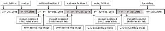
Figure 2.
Timetable of the experiment.
SPAD-502Plus Chlorophyll Meter was used to measure the SPAD values of naked barley leaves in the field. The meter has a measuring area of 2 mm × 3 mm and a measuring accuracy within 1.0 SPAD unit. The average SPAD value by 3 random measurements at different places in one leaf was used as the leaf’s measured SPAD value. The average SPAD value by 10 naked barley leaves in each group was used as the experimental group’s measured SPAD value.
DJI Phantom3 Professional (Da-Jiang Innovations Science and Technology Co., China) was the UAV system to acquire naked barley canopy images in the RGB wavelengths in this study. The camera uploaded on the UAV uses a 1/2.3 complementary metal-oxide-semiconductor (CMOS) with 12.4 megapixels (4000 × 3000) and the shooting direction is perpendicular to it. The field of view of the camera is 94°, the focal length is 20 mm, the f-number is f/2.8 and focus at the infinite point (∞). The camera uses automatic exposure during the image acquirement. The reflectance was not obtained by the reference normalization because the atmospheric effect was regarded very little due to the low flight heights in this study. Thus, the DN values of R, G and B channels of UAV images represented the relative radiance. The images were obtained at two different flight heights above ground level of 6.0 m and 50.0 m with an accuracy of flight altitude of 0.1 m. For the images at 6.0 m, each image only included one experimental group and there were no overlapped parts among different group images. Whereas the images at 50.0 m included all experimental groups (18 groups) for one day.
The measured SPAD value in the field and UAV images at 6.0 m and 50.0 m of one group were used as one set of data samples in the study. There were 18 samples per day and 4 flight days. Nevertheless, the data of ‘Repeat 2’ of ‘Group C’ on 8 December 2018 was deleted from the sample set because of the damaged UAV image at 6.0 m, so that the total sample number was 71.
2.3. Data Processing
2.3.1. Flowchart of Data Processing
The whole data processing was illustrated in Figure 3. Firstly, the image classification by Maximum likelihood classification (MLC) was conducted to extract vegetation parts on the UAV images of both flight heights; secondly, the naked barley ear was subsequently masked for the images at 6.0 m; thirdly, the VIs were calculated for the original, vegetation extracted without the ear masked and vegetation extracted with the ear masked images; fourthly, linear regression models were developed to relate the VIs with the field measured SPAD values; fifthly, the SPAD values prediction models were validated by an independent dataset; lastly, a robust VI for predicting SPAD values was selected for different photography conditions (including solar and flight height).

Figure 3.
Flowchart of the study.
2.3.2. Image Segmentation
MLC was used to extract the vegetation cover by classifying UAV-derived RGB images at both flight heights by the ENVI 5.5 (Harris Geospatial Solutions) software [49]. At first, for both flight heights, the UAV-images were classified into three categories: naked barley, soil and shadow. Then, the soil and shadow parts were masked and the vegetation cover was left in the images. Moreover, the naked barley ear was additionally masked after vegetation extraction for the images of 6.0 m flight height by ‘MLC’ and ‘Mask’ applications in ENVI 5.5 because the ear was very evident in the image of the lower flight height but was not detailed captured by the image of higher flight. Example images for image segmentation procedure at the flight height of 6.0 m are shown in Figure 4.
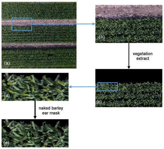
Figure 4.
Example images for image segmentation at the flight height of 6.0 m. (a) Unmanned Aerial Vehicle (UAV)-derived RGB image; (b) partially enlarged UAV-derived RGB image; (c) image of vegetation extraction by masking the soil and shadow; (d) partially zoom in for vegetation extraction result; (e) image after vegetation extraction and naked barley ear mask.
According to the different image segmentation procedure, there were five kinds of UAV images in our study: (1) original images at 6.0 m; (2) images by vegetation extraction but without naked barley ear mask processing at 6.0 m; (3) images by vegetation extraction with naked barley ear masked at 6.0 m; (4) original images at 50.0 m; and (5) images by vegetation extraction but without naked barley ear mask processing at 50.0 m.
2.3.3. Color-Based Vegetation Indices
A 5 m × 4.5 m image area was used for VIs calculation for each group. Due to the different photography area in one image at different flight heights, 3.6 megapixels (2000 × 1800) were used for each experimental group at 6.0 m flight height and 28.8 thousand pixels (180 × 160) were used for each group at 50.0 m flight height. The marginal areas of each group were cut from the images to eliminate the effect of fertilization on naked barley growth in different groups because the fertilization details were different among the neighboring groups. The cut-images would be called UAV images below.
Twenty one VIs derived from 2 color systems were calculated for all the UAV images. The VIs used in our study were shown in Table 2. For the images after vegetation extraction or naked barley mask, the masked pixels were excluded in the VIs calculation.
Table 2.
Color-based vegetation indices.
The RGB color system is the most common color system for the digital image. It describes one color by using three different (red, green, blue) values. The representation for the darkest black is (0, 0, 0) and the brightest white is (255, 255, 255) [50]. ‘R,’ ‘G’ and ‘B’ are the mean of the red, green and blue channels in UAV images [51]. ‘(R + G + B)/3’ is the average of ‘R,’ ‘G’ and ‘B’ values [17]. ‘R/(R + G + B),’ ‘G/(R + G + B),’ ‘B/(R + G + B)’ are normalized redness intensity, normalized greenness intensity and normalized blueness intensity, respectively [20]. ‘G/R,’ ‘B/G,’ ‘B/R’ are green-red ratio index, blue-green ration index and blue-red ratio index, respectively [22,52,53]. ‘G − B’ and ‘R − B’ are difference vegetation indices [20,21]. ‘2G − R − B’ is the excess green index [19]. ‘(R − B)/(R + B),’ ‘(G − B)/(G + B),’ ‘(G − R)/(G + R)’ are normalized red-blue difference index, normalized green-blue difference index and normalized green-red difference index, respectively [18,54,55]. ‘(2G − R − B)/(2G + R + B)’ is the visible-channel difference vegetation index [56].
The CIE L*a*b* color system is designed to approximate human vision. It describes color by three values: (1) L* represents the human perception of lightness from black (0) to white (100), (2) a* represents the visual perception from green (−a*) to red (+a*) and (3) b* means for the visual perception from blue (−b*) to yellow (+b*). L*, a* and b* are computed from tristimulus values X, Y and Z as following equations:
where , and describe a specified gray object-color stimulus [23,24,57].
2.3.4. Data Analysis
71 samples of ‘Repeat 1,’ ‘Repeat 2’ and ‘Repeat 3’ were used to detect the significance of one-way analysis of variance of SPAD values for different fertilizer treatments and growth stages after checking the normality assumption for groups and SPAD values at 0.05 probability level.
48 samples of ‘Repeat 1’ and ‘Repeat 3’ were used to detect the relationship between VIs and measured SPAD values by Pearson correlation and regression analyses after checking the normality assumption. Linear regression models were fitted to each VI. The significance of linear regressions was evaluated using Student’s t-test at 95% confidence levels. The data analysis was done by IBM SPSS Statistics (International Business Machines Corporation). 23 samples of ‘Repeat 2’ were used to validate regression models.
For each regression model, the root mean square error (RMSE) and normalized root mean square error (NRMSE) were used to validate using 23 samples of ‘Repeat 2.’ The equations of RMSE and NRMSE are presented in Equations (8) and (9).
in which, is the measured SPAD value of sample , is the predicted SPAD value of sample and is the number of validation samples.
3. Results
3.1. SPAD Values for Different Fertilizer Treatments
The measured SPAD values of each experimental group in the field at different dates were shown in Figure 5. The lowest SPAD value (26.30) occurred at Repeat 2, Group C, January 2019 and the highest (55.95) appeared at Repeat 1, Group C, March 2019. The SPAD value range was not much different from that in other researches, for example, 2~60 for sugar beet and 2.88~53.43 for potato [58,59]. For the SPAD values measured on the same date, the maximum difference occurred on 8 January 2019, from 26.30 (Repeat 2, Group C) to 36.30 (Repeat 1, Group B). The results of one-way analysis of variance of SPAD values for different fertilizer treatments and growth stages were shown in Table 3. Only the SPAD values in Jan. 2019 showed a significant difference for different fertilizer treatments. In contrast, there were significant differences among different growth stages for all fertilizer treatments. The overview for all experimental groups is displayed in Figure 6 by the UAV-RGB images derived at the flight height of 50.0 m. The parts corresponding to the low SPAD values showed light green, even close to yellow, while the regions with high SPAD values displayed green or dark green in the images (Figure 6). The maximum difference in the scene due to the fertilizer treatments occurred on 8 January 2019 (Figure 6b).

Figure 5.
Measured soil and plant analysis development (SPAD) values of each experimental group on 8 December 2018 (a); 8 January 2019 (b); 5 February 2019 (c) and 14 March 2019 (d).
Table 3.
The result of one-way analysis of variance of SPAD values for different fertilizer treatments and growth stages at 0.05 probability level.
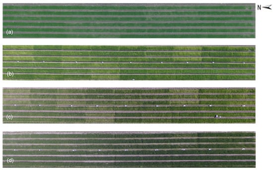
Figure 6.
UAV-derived RGB images at 50.0 m on 8 December 2018 (a); 8 January 2019 (b); 5 February 2019 (c) and 14 March 2019 (d).
However, there are some slight color differences among the same experimental groups on the same date or even in the same sample plot. Generally, the solid fertilizer used in our study can only be absorbed by the crop after being dissolved. Precipitation is one of the most critical impact factors on the degree of fertilizer dissolved under the rainwater irrigation system. Moreover, the naked barley growth density for different experimental groups in our study was not the same, caused by the inhomogeneity of nutrient, moisture and other soil characteristics. All these factors would lead to different fertilizer utilization rates of the naked barley, even for the same fertilizer treatment, in the field. Therefore, growth status variances occurred to the same fertilizer treatment experimental groups in our study and showed different greenness in the overview image on the same date.
3.2. Optimal Image Processing for Best Relating SPAD Values with Vegetation Indices
The VIs were calculated from the original image, the image with vegetation extraction without naked barley ears mask and the image with the vegetation extraction and naked barley ears mask, respectively, for the 6.0 m height images. Simultaneously, the vegetation indices were calculated only on the original image and the image with vegetation extraction for the 50.0 m height because the ears mask was not applied on it. Correlation between measured SPAD values and VIs of sample sets of ‘Repeat 1’ and ‘Repeat 3’ were displayed by correlation coefficient (r) in Table 4. The correlation coefficients after applying vegetation extraction were higher than that in the original imagery data for most VIs at both flight heights. Moreover, for the VIs calculated from UAV images at 6.0 m, the correlation coefficients showed even higher on the images after vegetation extraction and naked barley ears masked than that with the only vegetation extraction. In other words, the VIs had a better correlation with SPAD values of naked barley leaves after applying both vegetation extraction and naked barley ears masked.
Table 4.
Correlation coefficients between SPAD values and vegetation indices derived from UAV images.
3.3. Relationships between SPAD Values and Vegetation Indices
The different VIs showed various relationships with SPAD values. It seemed that most of the VIs did not perform consistently on the images from different flight heights. For the VIs derived from the image with vegetation extraction and naked barley ears mask at the flight height of 6.0 m, the index of ‘R,’ ‘G,’ ‘B,’ ‘L*,’ ‘b*,’ ‘b*/a*,’ ‘G − B,’ ‘R − B,’ ‘2G − R − B,’ ‘(R + G + B)/3’ and ‘R/(R + G + B)’ showed significant correlation with SPAD values of naked barley leaves (r > 0.70). For the VIs derived from the image with the processing of vegetation extraction at the flight height of 50.0 m, the index of ‘L*,’ ‘b*,’ ‘B/G,’ ‘G − B,’ ‘2G − R − B,’ ‘B/(R + G + B),’ ‘(G − B)/(G + B)’ and ‘(2G − R − B)/(2G + R + B)’ showed significant correlation with SPAD values of naked barley leaves (r > 0.70). The high correlation between these VIs and SPAD values at different flight heights suggested that the color-based VIs calculated from UAV images could indicate SPAD values of naked barley leaves, even at different photography conditions.
To determine a robust and generic vegetation index for SPAD values estimation on naked barley leaves for the images from different flight heights, we selected VIs that showed significant correlations with SPAD values at both flight heights to compare. The relationships between measured SPAD values and the index of ‘L*,’ ‘b*,’ ‘G − B’ and ‘2G − R − B’ calculated from the UAV image after vegetation extraction and naked barley ears mask at 6.0 m and 50.0 m were shown in Figure 7 and Figure 8, respectively. Among these 4 VIs in Figure 7 and Figure 8, the VI of ‘G − B’ performed the best correlation with SPAD values of naked barley leaves at both flight heights.
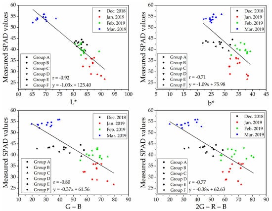
Figure 7.
Relationships between measured SPAD values and UAV images (with vegetation extraction and naked barley ear masked)-derived vegetation indices at the flight height of 6.0 m (n = 48).
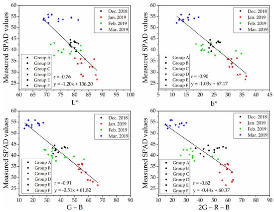
Figure 8.
Relationships between measured SPAD values and UAV images (with vegetation extraction but without naked barley ear masked)-derived vegetation indices at the flight height of 50.0 m (n = 48).
3.4. Validation of the Linear Regression Models for Predicting SPAD Values
The validation of the linear regression models for predicting SPAD values was conducted by an independent dataset of ‘Repeat 2’ (n = 23). The RMSE and NRMSE of regression models were shown in Table 5. The table suggested that the RMSE and NRMSE of the indices, which performed better correlations with SPAD values (Table 4), were lower than those which were not significantly correlated to SPAD values. The validations of the index of ‘L*,’ ‘b*,’ ‘G − B’ and ‘2G − R − B,’ which displayed significant correlations with SPAD values at 6.0 m (with vegetation extraction and naked barley ears mask) and 50.0 m (for the images with vegetation extraction only), were illustrated in Figure 9 for 6.0 m and Figure 10 for 50.0 m. For these 4 VIs, NRMSE varied from 8.79% to 16.06% at 6.0 m and from 6.51% to 17.77% at 50.0 m. Only the model of ‘G − B’ performed reasonably well at both flight heights. Therefore, the index of ‘G − B’ could be regarded as the robust vegetation index to estimate SPAD values of naked barley leaves independent of the flight heights and photography conditions.
Table 5.
RMSE (NRMSE) of the validation for SPAD values estimation with vegetation indices derived from UAV images.
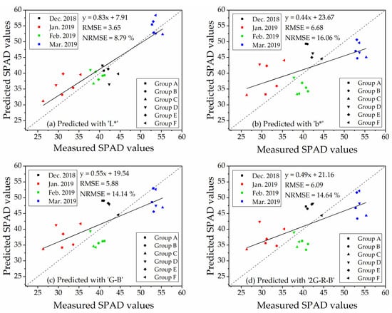
Figure 9.
Validation of the four models for estimating of SPAD values at the flight height of 6.0 m (n = 23).
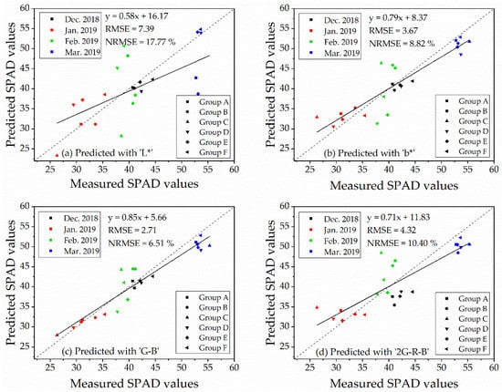
Figure 10.
Validation of the four models for estimating of SPAD values at the flight height of 50.0 m (n = 23).
Subsequently, we made distribution maps of estimated SPAD values (Figure 11) from overviewed UAV RGB image (vegetation extraction applied) at the flight height of 50.0 m via the linear regression equation derived from the measured SPAD values and the VI of ‘G − B.’ By comparing Figure 11 with Figure 6, we could find that the SPAD value image roughly corresponded to the colors and tones of the RGB image. The pixels with low SPAD values in Figure 11 corresponded to the light green area, even similar to yellow color, in Figure 6. The pixels with high SPAD values in Figure 11 corresponded to the green or dark green area in Figure 6.
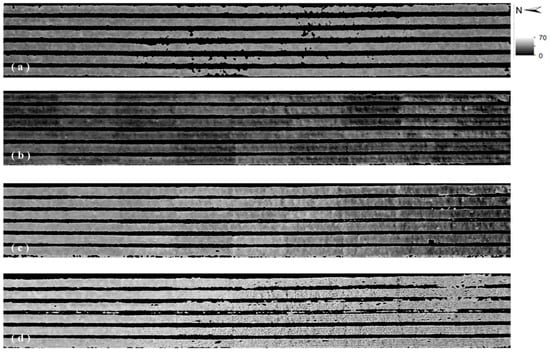
Figure 11.
Estimated SPAD value images at 50.0 m by using the VI of ‘G-B’ on 8 December 2018 (a); 8 January 2019 (b); 5 February 2019 (c) and 14 March 2019 (d).
4. Discussion
4.1. The SPAD Value Estimation Improvements by Vegetation Extraction and Naked Barley Ears Mask
The vegetation extraction and naked barley ears mask have improved the SPAD value estimation (Table 4) because they removed most of the soil, shadow and naked barley ears in the image. The soil, shadow and naked barley ears parts were considered as the background noise in our study because that they were irrelevant to SPAD values of naked barley and would affect the vegetation discrimination in the image [60,61]. Thus the image-based VIs can have a stronger correlation with SPAD values after the background was masked. Therefore, we consider that the vegetation extraction (soil and shadow masked) and naked barley ears mask as an optimal image processing method for correlating color-based vegetation indices calculated from UAV images with SPAD values of naked barley leaves.
4.2. Performance of the Color-Based VIs on Estimating SPAD Values
According to Table 4, we could find that very high differences occurred on the relationships between the SPAD values and the VIs of ‘R,’ ‘G’ and ‘B’ from images at different flight heights in our study. At the flight height of 6.0 m, correlation coefficients of the ‘R,’ ‘G’ and ‘B’ after vegetation extraction and naked barley ears mask were very high (‘−0.97,’ ‘−0.95’ and ‘−0.80’) but at the flight height of 50.0 m, they decreased to ‘−0.41,’ ‘−0.70’ and ‘0.33’ after vegetation extraction. In other words, there was a significant relationship between ‘R,’ ‘G,’ ‘B’ and SPAD values at 6.0 m but not a strong correlation at 50.0 m, especially for ‘R’ and ‘B.’ For the UAV images acquired at 50.0 m, the north area in the image showed a little higher brightness than the south area, especially for the image of February 2019 and March 2019 (Figure 6), which would lead to some errors in the image-based vegetation indices calculation on the images at 50.0 m height [62,63,64]. This inconsistent brightness in the whole image may be caused by the unstable flight status and camera’s internal parameter adjustment in a large photography area of the commercial digital camera mounted on the UAV in our study. The UAV images at 50.0 m in our study had a large image area, including the experimental area with low reflectance and some bare sandy soil with a high reflectance located in the north of our experimental area. In the south area of the image at 50.0 m, only farmland with low reflectance was included. For the north area in the image, the camera’s internal parameters might be difficult to adjust due to the clear difference in the brightness between the bare sandy soil and farmland in the north of the image, especially on clear days. Therefore, the inconsistent brightness occurred to the image at 50.0 m due to the digital camera’s internal parameter adjustment during photographing. However, for the images at 6.0 m, there was only the experimental area in each image. For the UAV images captured at the flight height of 6.0 m, compared to the images at 50.0 m, a smaller photographic area was performed in each image. There was only the experimental area in each image of 6.0 m. It may be easy for the commercial digital camera to adjust its internal parameters to a more suitable condition to acquire the image at a lower flight height. As a result, there was no apparent non-uniform brightness in the images at 6.0 m. Therefore, the distinctly inconsistent brightness throughout the whole RGB image at the flight height of 50.0 m could be considered as the reason for variances between the relationship of SPAD values and the index of ‘R,’ ‘G,’ ‘B’ in two different flight heights in our study.
For the color-based VIs calculated from UAV images at 6.0 m and 50.0 m, the index of ‘L*,’ ‘b*,’ ‘G − B’ and ‘2G − R − B’ performed significant correlations with SPAD values of naked barley leaves at these two flight heights in our study and ‘G−B’ was the most robust one among them. For the VIs of ‘G − B’ and ‘2G − R − B,’ they could be regarded as corrected values for the form of subtracting the ‘B’ channel value from the ‘G’ channel value or subtracting the ‘R’ and ‘B’ channel values from the ‘G’ channel value during the VI calculations. They may eliminate the brightness unbalance within one image for different experimental groups at 50.0 m height in our study. Consequently, the correlations between the index of ‘G − B’ and ‘2G − R − B’ with SPAD values were strong at 50.0 m, even under the whole image’s different brightness. Further research that focuses on the brightness calibration among whole UAV-derived images should be expected.
The index of ‘L*’ and ‘b*,’ which were based on CIE L*a*b* color system, also showed reasonable performance for estimating SPAD values. During the calculation from RGB values (Equations (1)–(7)), the ‘G’ value took up a large proportion of the index of ‘L*’ and the index of ‘b*’ responded to the index of ‘G − B’. Also, the index of ‘L*’ and ‘b*’ was divided by a gray board during calculating, which might normalize the index. Therefore, the index of ‘L*’ and ‘b*’ also performed significant correlations with SPAD values.
Moreover, for the relationship of ‘R,’ ‘G,’ ‘B’ indices with SPAD values of naked barley leaves in our study, there was also one more point that should be noted. The order of relevancy for these three single channels with SPAD values was not the same in our study’s two flight heights. The ‘R’ and ‘G’ had a much higher correlation with SPAD values than ‘B’ and ‘R’ was a little higher than ‘G’ for the UAV-image at the flight height of 6.0 m, whereas ‘G’ had much higher correlation than ‘R’ and ‘B’ and ‘R’ was a few higher than ‘B’ for the UAV-image at 50.0 m. Furthermore, neither of these two correlations was consistent with a previous study about correlation analysis of total chlorophyll content with ‘R,’ ‘G’ and ‘B’ indices, which were derived from the multispectral TV camera and conducted under constant lighting in the laboratory through various interference filters in a silicon vidicon camera [65]. The index of ‘B’ showed the best correlation and ‘R’ was the third in the previous study. Hunt has indicated that the vegetation indices, which usually showed good performance at the leaf scale, may not perform well at the canopy level [54]. Generally, the ‘B’ value of targets, one of the RGB color system parameters, seldom can be stably measured under solar light. The ‘B’ value is a channel easily affected by the atmospheric conditions because of the scattering; meanwhile, the ‘R’ and ‘G’ are not easily affected by atmospheric scattering when compared with the ‘B’ channel, especially on a clear day [66]. The indices used in our study were based on the UAV-derived images in the field under the sunlight. The reflected light from the naked barley canopy and the scattered light from the atmosphere were included during vegetation index calculation for the ‘B’ channel’s value. This would lower the precision of ‘B’ values in our images and lead to the instability of chlorophyll content estimation accuracy among different light sources during photography.
Although the commercial digital color camera has the advantages of low cost, convenient operation and simple data processing, exposure time and internal parameters adjustment, which would be set based on the weather conditions, would significantly affect image quality such as brightness and color temperature [67]. The unstable photographic condition, including weather and atmospheric conditions described above, may result in the instability of a single channel’s color-based index calculation. On the contrary, the vegetation indices of ‘G − B’ and ‘2G − R − B’, the adjusted indices, obtained a relatively high correlation with SPAD values of naked barley leaves in our study.
5. Conclusions
The present study suggested that the application of vegetation extraction and naked barley ears mask can improve the correlation between color-based vegetation indices calculated from UAV-mounted commercial digital camera and SPAD values of the naked barley leaves. Although vegetation indices had different correlations between SPAD values for different UAV flight heights and photography conditions, ‘L*,’ ‘b*,’ ‘G − B’ and ‘2G − R − B’ had significant correlations with SPAD values under different conditions. The index of ‘G − B’ can be regarded as the best vegetation index for estimating SPAD values of naked barley leaf from UAV-derived RGB images in our study because of the excellent performance in the validation. This vegetation index could be used for different photography conditions (including sunlight condition, camera’s internal parameter and UAV flight height).
This research provided a method to estimate SPAD values of naked barley in a wide range by UAV. The method could reduce the influence of UAV photography conditions, which can make environmental conditions for acquiring UAV images less strict and did not require multispectral or hyperspectral sensors, which are very high expenses for ordinary farmers. The commercial digital camera usage, which showed a reasonable estimation of SPAD values of the naked barley crop, could be regarded as a low-cost method. Hence, its affordability may increase its application in the crop monitoring practice.
From a longer-term perspective, more deeply research about the relationship between crop biophysical parameters (not only SPAD values but also above-ground biomass, yield and so on) and color-based vegetation indices derived from UAV-mounted commercial digital camera and crop biophysical parameters is expected.
Author Contributions
Y.L., K.H. and K.O. designed the experiment; Y.L., K.H., T.A. (Takanori Aihara), S.K., T.A. (Tsutomu Akiyama) and Y.K. performed the experiment; Y.L., K.H., S.L. and K.O. performed the data analysis, Y.L., K.H. and T.A. (Takanori Aihara) prepared the original draft; and K.O. and S.L. revised. All authors have read and agreed to the published version of the manuscript.
Funding
This research received no external funding.
Conflicts of Interest
The authors declare no conflict of interest.
References
- Food and Agriculture Organization of the United Nations. Available online: http://www.fao.org/faostat/zh/#data/QC/visualize (accessed on 22 December 2020).
- Vinesh, B.; Prasad, L.; Prasad, R.; Madhukar, K. Association studies of yield and it’s attributing traits in indigenous and exotic Barley (Hordeum vulgare L.) germplasm. J. Pharmacogn. Phytochem. 2018, 7, 1500–1502. [Google Scholar]
- Agegnehu, G.; Nelson, P.N.; Bird, M.I. Crop yield, plant nutrient uptake and soil physicochemical properties under organic soil amendments and nitrogen fertilization on Nitisols. Soil Tillage Res. 2016, 160, 1–13. [Google Scholar] [CrossRef]
- Spaner, D.; Todd, A.G.; Navabi, A.; McKenzie, D.B.; Goonewardene, L.A. Can leaf chlorophyll measures at differing growth stages be used as an indicator of winter wheat and spring barley nitrogen requirements in eastern Canada? J. Agron. Crop Sci. 2005, 191, 393–399. [Google Scholar] [CrossRef]
- Houles, V.; Guerif, M.; Mary, B. Elaboration of a nitrogen nutrition indicator for winter wheat based on leaf area index and chlorophyll content for making nitrogen recommendations. Eur. J. Agron. 2007, 27, 1–11. [Google Scholar] [CrossRef]
- Clevers, J.G.P.W.; Kooistra, L. Using hyperspectral remote sensing data for retrieving canopy chlorophyll and nitrogen content. IEEE J. Sel. Top. Appl. Earth Obs. Remote Sens. 2011, 5, 574–583. [Google Scholar] [CrossRef]
- Yu, K.; Lenz-Wiedemann, V.; Chen, X.; Bareth, G. Estimating leaf chlorophyll of barley at different growth stages using spectral indices to reduce soil background and canopy structure effects. ISPRS J. Photogramm. Remote Sens. 2014, 97, 58–77. [Google Scholar] [CrossRef]
- Shah, S.H.; Houborg, R.; McCabe, M.F. Response of chlorophyll, carotenoid and SPAD-502 measurement to salinity and nutrient stress in wheat (Triticum aestivum L.). Agronmy 2017, 7, 61. [Google Scholar] [CrossRef]
- Follett, R.; Follett, R.; Halvorson, A. Use of a chlorophyll meter to evaluate the nitrogen status of dryland winter wheat. Commun. Soil Sci. Plant Anal. 1992, 23, 687–697. [Google Scholar] [CrossRef]
- Li, G.; Ding, Y.; Xue, L.; Wang, S. Research progress on diagnosis of nitrogen nutrition and fertilization recommendation for rice by use chlorophyll meter. Plant Nutr. Fert. Sci. 2005, 11, 412–416. [Google Scholar]
- Lu, X.; Lu, S. Effects of adaxial and abaxial surface on the estimation of leaf chlorophyll content using hyperspectral vegetation indices. Int. J. Remote Sens. 2015, 36, 1447–1469. [Google Scholar] [CrossRef]
- Jiang, C.; Johkan, M.; Hohjo, M.; Tsukagoshi, S.; Maruo, T. A correlation analysis on chlorophyll content and SPAD value in tomato leaves. HortResearch 2017, 71, 37–42. [Google Scholar]
- Minolta, C. Manual for Chlorophyll Meter SPAD-502 Plus; Minolta Camera Co.: Osaka, Japan, 2013. [Google Scholar]
- Pagola, M.; Ortiz, R.; Irigoyen, I.; Bustince, H.; Barrenechea, E.; Aparicio-Tejo, P.; Lamsfus, C.; Lasa, B. New method to assess barley nitrogen nutrition status based on image colour analysis: Comparison with SPAD-502. Comput. Electron. Agr. 2009, 65, 213–218. [Google Scholar] [CrossRef]
- Golzarian, M.R.; Frick, R.A. Classification of images of wheat, ryegrass and brome grass species at early growth stages using principal component analysis. Plant Methods 2011, 7, 28. [Google Scholar] [CrossRef]
- Rorie, R.L.; Purcell, L.C.; Mozaffari, M.; Karcher, D.E.; King, C.A.; Marsh, M.C.; Longer, D.E. Association of “greenness” in corn with yield and leaf nitrogen concentration. Agron. J. 2011, 103, 529–535. [Google Scholar] [CrossRef]
- Wang, Y.; Wang, D.; Shi, P.; Omasa, K. Estimating rice chlorophyll content and leaf nitrogen concentration with a digital still color camera under natural light. Plant Methods 2014, 10, 36. [Google Scholar] [CrossRef]
- Peñuelas, J.; Gamon, A.; Fredeen, A.; Merino, J.; Field, C. Reflectance indices associated with physiological changes in nitrogen-and water-limited sunflower leaves. Remote Sens. Environ. 1994, 48, 135–146. [Google Scholar] [CrossRef]
- Woebbecke, D.M.; Meyer, G.E.; Von Bargen, K.; Mortensen, D.A. Color indices for weed identification under various soil, residue, and lighting conditions. Trans. ASAE 1995, 38, 259–269. [Google Scholar] [CrossRef]
- Kawashima, S.; Nakatani, M. An algorithm for estimating chlorophyll content in leaves using a video camera. Ann. Bot. 1998, 81, 49–54. [Google Scholar] [CrossRef]
- Wang, F.; Wang, K.; Li, S.; Chen, B.; Chen, J. Estimation of chlorophyll and nitrogen contents in cotton leaves using digital camera and imaging spectrometer. Acta Agron. Sin. 2010, 36, 1981–1989. [Google Scholar]
- Wei, Q.; Li, L.; Ren, T.; Wang, Z.; Wang, S.; Li, X.; Cong, R.; Lu, J. Diagnosing nitrogen nutrition status of winter rapeseed via digital image processing technique. Sci. Agric. Sin. 2015, 48, 3877–3886. [Google Scholar]
- Graeff, S.; Pfenning, J.; Claupein, W.; Liebig, H.-P. Evaluation of image analysis to determine the N-fertilizer demand of broccoli plants (Brassica oleracea convar. botrytis var. italica). Adv. Opt. Technol. 2008, 2008, 359760. [Google Scholar] [CrossRef]
- Wiwart, M.; Fordoński, G.; Żuk-Gołaszewska, K.; Suchowilska, E. Early diagnostics of macronutrient deficiencies in three legume species by color image analysis. Comput. Electron. Agr. 2009, 65, 125–132. [Google Scholar] [CrossRef]
- Sulistyo, S.B.; Woo, W.L.; Dlay, S.S. Regularized neural networks fusion and genetic algorithm based on-field nitrogen status estimation of wheat plants. IEEE Trans. Ind. Informat. 2016, 13, 103–114. [Google Scholar] [CrossRef]
- Kanning, M.; Kühling, I.; Trautz, D.; Jarmer, T. High-resolution UAV-based hyperspectral imagery for LAI and chlorophyll estimations from wheat for yield prediction. Remote Sens. 2018, 10, 2000. [Google Scholar] [CrossRef]
- Hunt Jr, E.R.; Daughtry, C.S. What good are unmanned aircraft systems for agricultural remote sensing and precision agriculture? Int. J. Remote Sens. 2018, 39, 5345–5376. [Google Scholar] [CrossRef]
- Guo, Y.; Senthilnath, J.; Wu, W.; Zhang, X.; Zeng, Z.; Huang, H. Radiometric calibration for multispectral camera of different imaging conditions mounted on a UAV platform. Sustainability 2019, 11, 978. [Google Scholar] [CrossRef]
- Han-Ya, I.; Ishii, K.; Noguchi, N. Satellite and aerial remote sensing for production estimates and crop assessment. Environ. Control. Biol. 2010, 48, 51–58. [Google Scholar] [CrossRef]
- Gevaert, C.M.; Suomalainen, J.; Tang, J.; Kooistra, L. Generation of spectral–temporal response surfaces by combining multispectral satellite and hyperspectral UAV imagery for precision agriculture applications. IEEE J. Sel. Top. Appl. Earth Obs. Remote Sens. 2015, 8, 3140–3146. [Google Scholar] [CrossRef]
- Yue, J.; Yang, G.; Li, C.; Li, Z.; Wang, Y.; Feng, H.; Xu, B. Estimation of winter wheat above-ground biomass using unmanned aerial vehicle-based snapshot hyperspectral sensor and crop height improved models. Remote Sens. 2017, 9, 708. [Google Scholar] [CrossRef]
- Zheng, H.; Cheng, T.; Li, D.; Zhou, X.; Yao, X.; Tian, Y.; Cao, W.; Zhu, Y. Evaluation of RGB, color-infrared and multispectral images acquired from unmanned aerial systems for the estimation of nitrogen accumulation in rice. Remote Sens. 2018, 10, 824. [Google Scholar] [CrossRef]
- Teng, P.; Zhang, Y.; Shimizu, Y.; Hosoi, F.; Omasa, K. Accuracy assessment in 3D remote sensing of rice plants in paddy field using a small UAV. Eco-Engineering 2016, 28, 107–112. [Google Scholar]
- Teng, P.; Ono, E.; Zhang, Y.; Aono, M.; Shimizu, Y.; Hosoi, F.; Omasa, K. Estimation of ground surface and accuracy assessments of growth parameters for a sweet potato community in ridge cultivation. Remote Sens. 2019, 11, 1487. [Google Scholar] [CrossRef]
- Liebisch, F.; Kirchgessner, N.; Schneider, D.; Walter, A.; Hund, A. Remote, aerial phenotyping of maize traits with a mobile multi-sensor approach. Plant Methods 2015, 11, 9. [Google Scholar] [CrossRef] [PubMed]
- Candiago, S.; Remondino, F.; De Giglio, M.; Dubbini, M.; Gattelli, M. Evaluating multispectral images and vegetation indices for precision farming applications from UAV images. Remote Sens. 2015, 7, 4026–4047. [Google Scholar] [CrossRef]
- Lu, N.; Zhou, J.; Han, Z.; Li, D.; Cao, Q.; Yao, X.; Tian, Y.; Zhu, Y.; Cao, W.; Cheng, T. Improved estimation of aboveground biomass in wheat from RGB imagery and point cloud data acquired with a low-cost unmanned aerial vehicle system. Plant Methods 2019, 15, 17. [Google Scholar] [CrossRef] [PubMed]
- Shimojima, K.; Ogawa, S.; Naito, H.; Valencia, M.O.; Shimizu, Y.; Hosoi, F.; Uga, Y.; Ishitani, M.; Selvaraj, M.G.; Omasa, K. Comparison between rice plant traits and color indices calculated from UAV remote sensing images. Eco-Engineering 2017, 29, 11–16. [Google Scholar]
- Escalante, H.; Rodríguez-Sánchez, S.; Jiménez-Lizárraga, M.; Morales-Reyes, A.; De La Calleja, J.; Vazquez, R. Barley yield and fertilization analysis from UAV imagery: A deep learning approach. Int. J. Remote Sens. 2019, 40, 2493–2516. [Google Scholar] [CrossRef]
- Bendig, J.; Bolten, A.; Bennertz, S.; Broscheit, J.; Eichfuss, S.; Bareth, G. Estimating biomass of barley using crop surface models (CSMs) derived from UAV-based RGB imaging. Remote Sens. 2014, 6, 10395–10412. [Google Scholar] [CrossRef]
- Bendig, J.; Yu, K.; Aasen, H.; Bolten, A.; Bennertz, S.; Broscheit, J.; Gnyp, M.L.; Bareth, G. Combining UAV-based plant height from crop surface models, visible, and near infrared vegetation indices for biomass monitoring in barley. Int. J. Appl. Earth Obs. 2015, 39, 79–87. [Google Scholar] [CrossRef]
- Holman, F.H.; Riche, A.B.; Michalski, A.; Castle, M.; Wooster, M.J.; Hawkesford, M.J. High throughput field phenotyping of wheat plant height and growth rate in field plot trials using UAV based remote sensing. Remote Sens. 2016, 8, 1031. [Google Scholar] [CrossRef]
- Li, J.; Shi, Y.; Veeranampalayam-Sivakumar, A.-N.; Schachtman, D.P. Elucidating sorghum biomass, nitrogen and chlorophyll contents with spectral and morphological traits derived from unmanned aircraft system. Front. Plant Sci. 2018, 9, 1406. [Google Scholar] [CrossRef]
- Wang, Y.; Zhang, K.; Tang, C.; Cao, Q.; Tian, Y.; Zhu, Y.; Cao, W.; Liu, X. Estimation of rice growth parameters based on linear mixed-effect model using multispectral images from fixed-wing unmanned aerial vehicles. Remote Sens. 2019, 11, 1371–1392. [Google Scholar] [CrossRef]
- Mincato, R.L.; Parreiras, T.C.; Lense, G.H.E.; Moreira, R.S.; Santana, D.B. Using unmanned aerial vehicle and machine learning algorithm to monitor leaf nitrogen in coffee. Coffee Sci. 2020, 15, 1–9. [Google Scholar]
- Mesas-Carrascosa, F.-J.; Torres-Sánchez, J.; Clavero-Rumbao, I.; García-Ferrer, A.; Peña, J.-M.; Borra-Serrano, I.; López-Granados, F. Assessing optimal flight parameters for generating accurate multispectral orthomosaicks by UAV to support site-specific crop management. Remote Sens. 2015, 7, 12793–12814. [Google Scholar] [CrossRef]
- Avtar, R.; Suab, S.A.; Syukur, M.S.; Korom, A.; Umarhadi, D.A.; Yunus, A.P. Assessing the influence of UAV altitude on extracted biophysical parameters of young oil palm. Remote Sens. 2020, 12, 3030. [Google Scholar] [CrossRef]
- Meier, U. Growth stages of mono-and dicotyledonous plants. In BCH-Monograph, Federal Biological Research Centre for Agriculture and Forestry; Blackwell Science: Berlin, Germany, 2001. [Google Scholar]
- Lu, S.; Oki, K.; Shimizu, Y.; Omasa, K. Comparison between several feature extraction/classification methods for mapping complicated agricultural land use patches using airborne hyperspectral data. Int. J. Remote Sens. 2007, 28, 963–984. [Google Scholar] [CrossRef]
- Robertson, A.R. The CIE 1976 color-difference formulae. Color Res. Appl. 1977, 2, 7–11. [Google Scholar] [CrossRef]
- Pearson, R.L.; Miller, L.D.; Tucker, C.J. Hand-held spectral radiometer to estimate gramineous biomass. Appl. Opt. 1976, 15, 416–418. [Google Scholar] [CrossRef] [PubMed]
- Gamon, J.; Surfus, J. Assessing leaf pigment content and activity with a reflectometer. New Phytol. 1999, 143, 105–117. [Google Scholar] [CrossRef]
- Sellaro, R.; Crepy, M.; Trupkin, S.A.; Karayekov, E.; Buchovsky, A.S.; Rossi, C.; Casal, J.J. Cryptochrome as a sensor of the blue/green ratio of natural radiation in Arabidopsis. Plant Physiol. 2010, 154, 401–409. [Google Scholar] [CrossRef] [PubMed]
- Hunt, E.R.; Cavigelli, M.; Daughtry, C.S.; Mcmurtrey, J.E.; Walthall, C.L. Evaluation of digital photography from model aircraft for remote sensing of crop biomass and nitrogen status. Precis. Agric. 2005, 6, 359–378. [Google Scholar] [CrossRef]
- Gitelson, A.A.; Kaufman, Y.J.; Stark, R.; Rundquist, D. Novel algorithms for remote estimation of vegetation fraction. Remote Sens. Environ. 2002, 80, 76–87. [Google Scholar] [CrossRef]
- Wang, X.; Wang, M.; Wang, S.; Wu, Y. Extraction of vegetation information from visible unmanned aerial vehicle images. Trans. Chin. Soc. Agric. Eng 2015, 31, 152–159. [Google Scholar]
- Kirillova, N.; Vodyanitskii, Y.N.; Sileva, T. Conversion of soil color parameters from the Munsell system to the CIE-L* a* b* system. Eurasian Soil Sci. 2015, 48, 468–475. [Google Scholar] [CrossRef]
- Moghaddam, P.A.; Derafshi, M.H.; Shirzad, V. Estimation of single leaf chlorophyll content in sugar beet using machine vision. Turk. J. Agrci. For 2011, 35, 563–568. [Google Scholar]
- El-Mageed, A.; Ibrahim, M.; Elbeltagi, A. The effect of water stress on nitrogen status as well as water use efficiency of potato crop under drip irrigation system. Misr J. Ag. Eng. 2017, 34, 1351–1374. [Google Scholar] [CrossRef]
- Huete, A.; Post, D.; Jackson, R. Soil spectral effects on 4-space vegetation discrimination. Remote Sens. Environ. 1984, 15, 155–165. [Google Scholar] [CrossRef]
- Zhang, X.; Zhang, F.; Qi, Y.; Deng, L.; Wang, X.; Yang, S. New research methods for vegetation information extraction based on visible light remote sensing images from an unmanned aerial vehicle (UAV). Int. J. Appl. Earth Obs. 2019, 78, 215–226. [Google Scholar] [CrossRef]
- Hanan, N.; Prince, S.; Hiernaux, P.H. Spectral modelling of multicomponent landscapes in the Sahel. Int. J. Remote Sens. 1991, 12, 1243–4258. [Google Scholar] [CrossRef]
- Jiang, Z.; Huete, A.R.; Chen, J.; Chen, Y.; Li, J.; Yan, G.; Zhang, X. Analysis of NDVI and scaled difference vegetation index retrievals of vegetation fraction. Remote Sens. Environ. 2006, 101, 366–378. [Google Scholar] [CrossRef]
- Du, M.; Noguchi, N. Monitoring of wheat growth status and mapping of wheat yield’s within-field spatial variations using color images acquired from UAV-camera system. Remote Sens. 2017, 9, 289. [Google Scholar] [CrossRef]
- Omasa, K. Image instrumentation methods of plant analysis. In Physical Methods in Plant Sciences; Springer: Berlin/Heidelberg, Germany, 1990; Volume 11, pp. 203–243. [Google Scholar]
- Chavez Jr, P.S. An improved dark-object subtraction technique for atmospheric scattering correction of multispectral data. Remote Sens. Environ. 1988, 24, 459–479. [Google Scholar] [CrossRef]
- Yang, G.; Liu, J.; Zhao, C.; Li, Z.; Huang, Y.; Yu, H.; Xu, B.; Yang, X.; Zhu, D.; Zhang, X. Unmanned aerial vehicle remote sensing for field-based crop phenotyping: Current status and perspectives. Front. Plant Sci. 2017, 8, 1111. [Google Scholar] [CrossRef]


Publisher’s Note: MDPI stays neutral with regard to jurisdictional claims in published maps and institutional affiliations. |
© 2021 by the authors. Licensee MDPI, Basel, Switzerland. This article is an open access article distributed under the terms and conditions of the Creative Commons Attribution (CC BY) license (http://creativecommons.org/licenses/by/4.0/).