Article

Long-Term Trends in Root-Zone Soil Moisture across CONUS Connected to ENSO

1
Center for Earth and Environmental Studies, Texas A&M International University, Laredo, TX 78041-1900, USA
2
US Department of Agriculture Hydrology and Remote Sensing Laboratory, Beltsville, MD 20705, USA
*
Author to whom correspondence should be addressed.
Remote Sens. 2020, 12(12), 2037; https://doi.org/10.3390/rs12122037
Submission received: 17 April 2020 / Revised: 5 June 2020 / Accepted: 22 June 2020 / Published: 24 June 2020
(This article belongs to the Section Environmental Remote Sensing)

Abstract

:
Root zone soil moisture (RZSM) is one of the least-monitored variables within the hydrologic cycle. Given the importance of RZSM to agriculture, more effort is needed to understand the potential impacts of the El Niño southern oscillation (ENSO), Pacific decadal oscillation (PDO), and Atlantic multidecadal oscillation (AMO) on this critical variable. This study focused on the CONtiguous United States (CONUS) RZSM (0 to 40 cm depth) over nearly three decades (1992 to 2018). Basic trend analysis with the Mann–Kendall test and wavelet transform coherence (WTC) was utilized. The RZSM product examined was Soil MERGE (SMERGE 2.0). More CONUS pixels exhibited drying (56 to 75%) versus wetting (25 to 44%) trends between 1992 and 2018. Seasonal wetting trends were observed particularly during winter in the Southwest and Northwest regions associated with El Nino and La Nina episodes, respectively. The noted long-term RZSM trends are more clearly attributable to oceanic-atmospheric teleconnections than global climate change. The most significant result was the strong drying trend in central CONUS reflected a shift to La Nina and cool PDO conditions during the 2000s, further amplified by a change to positive AMO corresponding with this period.

1. Introduction

Root zone soil moisture (RZSM) is a key variable that controls the rainfall–runoff relationship and mediates the impact of water limitations on evapotranspiration at a watershed scale. As such, RZSM plays a pivotal role in modulating terrestrial water and energy fluxes [1]. However, RZSM is one of the least-monitored variables within the hydrologic cycle. Traditionally, RZSM has been monitored with in situ measurements which might not be representative over larger spatial scales [2]. The direct remote sensing of RZSM is a long-term goal of the community that has yet to be achieved. Preliminary RZSM results from NASA’s Airborne Microwave Observatory of Subcanopy and Subsurface (AirMOSS) initiative were a step in this direction [3]; yet, at present, no clear path exists for continuous space-based monitoring of this variable. Land surface models can provide spatially continuous estimates of RZSM; however, their output can be strongly influenced by errors in forcing data [4,5].
Given the importance of soil moisture to agricultural and water resource applications, more effort is needed to understand the impacts of climate change on trends in RZSM. Previous efforts have connected long-term changes in the terrestrial hydrologic cycle to anthropogenic forcing [6,7,8,9]. However, a problem with linking any long-term trend to climate change is that natural cyclic processes may mask the signal. A prime example of this is the El Niño Southern Oscillation (ENSO); an ocean phenomenon localized in the eastern equatorial Pacific with a pronounced two to seven year periodicity. The impact of ENSO on soil moisture has been studied using data from space-based remote sensing [10], sparse in situ sites [11], or model-based estimates of RZSM [12,13,14,15,16]. In this unique contribution, a recently developed RZSM product (Soil MERGE or SMERGE) that optimally leverages remotely sensed and land surface modeled data [17] was used to examine trends in RZSM between 1992 and 2018. As such, SMERGE combines the strengths of remote sensing and land surface modeling approaches. Additionally, this product facilitated an examination of RZSM across all of the conterminous United States (CONUS)—unlike most other studies that were limited to a specific watershed or region [12,13,14,15,16]. Therefore, the research objectives of this study were to identify trends in RZSM across CONUS from 1992 to 2018 and to link these trends with potential causal mechanisms. The remainder of this paper discusses the datasets utilized (Section 2), methodologies applied (Section 3), results obtained (Section 4), discussion (Section 5), and key conclusions (Section 6).

2. Dataset Description

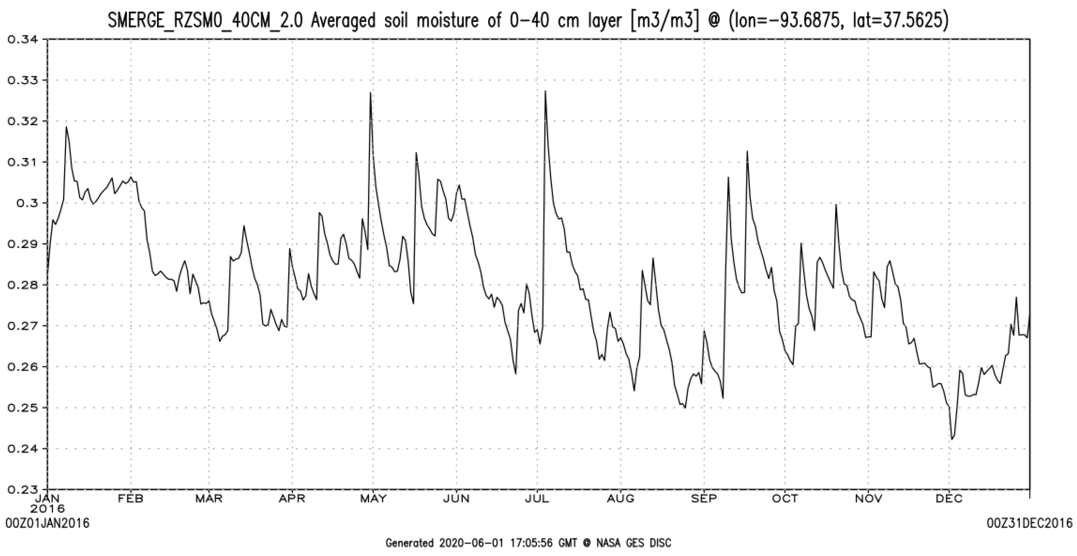
2.1. Root Zone Soil Moisture (RZSM)

SMERGE 2.0 combined two RZSM inputs for the 1992 to 2018 period. (1) Land surface model estimates acquired from Noah Land Surface Model (version 2.8) produced by the North American Land Data Assimilation System, Phase 2 (NLDAS-2, NOAH0125_H.002; DOI 10.5067/47Z13FNQODKV), which is referred to as NLDAS Noah. (2) Satellite-based soil moisture retrievals obtained from the European Space Agency Climate Change Initiative (ESA-CCI) Combined Version 3.3). The merger of these products produced a 0.125-degree, daily, shallow (0 to 40 cm) RZSM product within the conterminous United States (CONUS). The weighting procedure utilized in the combining the two parent inputs to make SMERGE RZSM was detailed in [17]. Additional details about NLDAS Noah and ESA-CCI Combined products are given below. An example of a time series for the SMERGE RZSM product is given in Figure 1.
NLDAS Noah is a daily product with a 0.125-degree spatial resolution [18]. Data from the top two layers (0 to 10 cm; 10 to 40 cm) of this model were combined by simple weighted averaging generating an estimate of overall soil moisture for the shallow root zone (0 to 40 cm). Noah version 2.8 was selected as the backbone for SMERGE 2.0 RZSM because of its consistent performance across CONUS [19].
The ESA-CCI Combined product represented a surface (0–5 cm) soil moisture retrieval. This product combines retrievals from active and passive microwave orbiting sensors. [20] described the harmonization procedure used to generate this dataset. The ESA-CCI Combined product is a daily product with a courser 0.25-degree spatial resolution compared with NLDAS-2 Noah. [17] described in detail how ESA-CCI surface soil moisture is converted into an estimate of RZSM between 0 and 40 cm. Basically, the approach used the exponential filter [21,22] combined with bilinear interpolation to fill in temporal data gaps.

2.2. Normalized Difference Vegetation Index (NDVI)

The normalized difference vegetation index, third generation using the Global Inventory Monitoring and Modeling System (GIMMS) from 1992 to 2015 was selected [23] to provide an independent estimate of land surface conditions across CONUS. This vegetation index reflects a corrected composite from an array of advanced very high-resolution radiometer (AVHRR) sensors, which is referred to below as AVHRR NDVI. The product is daily and has a 0.125-degree spatial resolution similar to SMERGE 2.0 RZSM.

2.3. ENSO, PDO, and AMO Indices

National Weather Service, Climate Prediction Center ENSO indices for cold and warm episodes for the period 1992–2018 were used in this study (Table 1). The episodes are defined based on a “threshold of ± 0.5 °C for the oceanic Niño index, which is a three-month running mean of Extended Reconstructed Sea Surface Temperature anomalies in the Niño 3.4 region (5°N–5°S, 120°–170°W) based on the 1971–1999 base period” (NOAA, 2005). El Niño, La Niña, and neutral episodes were designated based on the average seasonal sea water temperature for northern hemisphere winter (DJF), spring (MAM), summer (JJA), and fall (SON) seasons. The only significant protracted periods of warm Pacific decadal oscillation (PDO) anomalies (based on the same 0.5 °C threshold as ENSO) corresponded with most of 1992 to early 1994, the mid-1997 to early 1998 strong El Niño episode, and 2014 to 2016. Several studies [24,25] have indicated that, during the late 1990s, there was a general shift to cool-PDO conditions. These conditions dominated during the following years (late 1998 to 2002 and 2005 to 2014). Finally, the Atlantic multidecadal oscillation (AMO) recorded negative anomalies from 1992 to early 1997 and turned mainly positive afterward through 2018 [26].

3. Methods

Our approach is twofold. (1) To examine the long-term RZSM anomaly record across CONUS to determine regions with significant drying and wetting trends and (2) to use wavelet transform coherence (WTC) to elucidate connections between RZSM and ENSO based on sampled ranked correlation coefficients at 61 sites scattered across CONUS that have a robust record of in situ RZSM observations [17].

3.1. Trend Analysis

The Mann–Kendall test has been widely used to discern the significance of monotonic trends present in hydrological and hydrometeorological time series datasets [27,28]. This is a nonparametric test supporting the analysis of data distributions that do not necessarily have a normal distribution. The test compares a time series against a null hypothesis where the data was distributed so that there was no trend. The Mann–Kendall test has been commonly applied in the analysis of precipitation time series e.g., [29,30,31,32,33] and streamflow [34]. However, application of this test for soil moisture datasets has been more limited e.g., [35] especially for RZSM [36]. Trend analysis was conducted at a seasonal time scale corresponding with northern hemisphere winter (DJF), spring (MAM), summer (JJA), and fall (SON), and focused on RZSM anomalies.
To document teleconnections (sea surface temperature indexes lagged –12 months compared with RZSM anomalies) based on the Multivariate ENSO Index Version 2 (MEI.v2; El Niño, La Niña, neutral) was utilized. This approach calculates trends for each specific ENSO phase and each season. Since hydrologic response occurs up to 12 months behind atmospheric forcing [12], the lagged analysis approach is justified. Analysis for a specific ENSO phase was completed only if at least six years of that phase were available. This eliminated MAM from both El Nino and La Nina from consideration.
Finally, trend analysis of AVHRR NDVI (no lag and +1 month lag) at the above seasonal timescales were completed for comparison purposes. Across CONUS, we have noted a nominal one-month lag between RZSM and vegetation response [17]. All datasets examined the period 1992 to 2018 except NDVI, which is limited to the period between 1992 and 2015 by the availability of this product. Percentage of pixels with drying (wetting) trends and absolute trend correlation (r value), based on the linear trend between RZSM anomalies and time, were used for evaluation. Analysis included all CONUS pixels and only pixels that exhibited a significant trend (P < 0.10). Additionally, the distribution of r values was examined. Finally, to provide a more focused analysis, trends were examined within four CONUS states that have a particularly strong response to ENSO, PDO, and AMO (Arizona, Georgia, Iowa, Texas).

3.2. Wavelet Transform Analysis

Wavelet transform coherence (WTC) elucidated teleconnections present between ENSO and RZSM anomalies [37]. This approach has been used in previous studies examining trends in soil moisture and groundwater [15,38]. We applied WTC to a total of 77 time series from 61 sites. Locations corresponded with Soil Climate Analysis Network (SCAN) and the U.S. Climate Reference Network (USCRN) sites across CONUS that have been previously screened [17] as having at least five years of reasonable complete and accurate in situ RZSM data (Figure 2).
WTC analysis allowed us to determine the periodicity at which ENSO was modulating RZSM across CONUS between 1992 and 2018. The continuous WTC method selected was an appropriate choice to analyze nonstationary signals like soil moisture. In addition, this method identified the time scale associated with forcing events that produced nonstationary signals. Specifically, the Morse wavelet transform applied was appropriate for analyzing signals with time-varying amplitude and frequency. Also, this approach was useful for analyzing datasets with localized discontinuities. This approach has the advantage that it is a balanced method that allows for delineation of variability properties based on both time and frequency and is adept at capturing the oscillatory characteristics of a dynamic system. A Spearman’s rank correlation coefficient was applied to determine the rank correlation (R value) of the two-time series. The scale-averaged wavelet power was determined by analysis of ENSO versus RZSM anomalies (and NDVI) at 61 sites (77 time series) scattered across CONUS (Figure 2).

4. Results

4.1. Trend Analysis

CONUS-wide, the number of pixels with a long-term drying trend outnumbers those with a wetting trend for SMERGE 2.0 RZSM (Table 2). This tendency was more evident when examining pixels that have a significant trend and was particularly pronounced during JJA, where the number of pixels with a significant drying trend exceeded wetting by almost 50% of CONUS. The drying tendency was mirrored by AVHRR NVDI retrievals that records significant browning, especially during the warm season across CONUS (Table 2). For all seasons, the absolute r values yielded from trend analysis for all CONUS pixels on a seasonal basis were higher when focusing on significant pixels (p < 0.10; average r = 0.4 to 0.5) as opposed to all CONUS pixels (average r = 0.2 to 0.3). A more detailed analysis by season and ENSO phase follows.

4.1.1. Winter (DJF)

During winter (DJF) there were a greater number of pixels that exhibit drying (browning) versus wetting (greening) for all products (Table 2). Overall spatial variations of these trends were as follows. SMERGE 2.0 RZSM had scattered significant drying localized in the central Mississippi Valley and California (Figure 3a). In addition, drying was noted in the Northern Plains (Minnesota and the Dakotas). One-month lagged NVDI AVHRR had a greater number of significant pixels with scattered browning and greening across all of CONUS (Table 2). A coherent area of browning extended from the Great Plains (Kansas) eastward into the Great Lakes region (Michigan; Figure 3b).
Examination of spatial trends based on ENSO phase provided a more nuanced portrayal. High absolute r values obtained from trend analysis were noted for each ENSO phase (CONUS-wide average = 0.3 to 0.4; significant pixels average = 0.7; Figure 4a). During El Nino episodes, SMERGE 2.0 RZSM had significant wetting in the Southwest and drying along the Pacific Northwest coast and in an area that extended from the central Mississippi Valley into the Mid-Atlantic states (Figure 3c). La Nina phases exhibited discontinuous areas of wetting scattered across the Northwest (Figure 3d). Finally, during neutral phases, there were a fewer number of significant pixels (Table 2), and no coherent large-scale regional trends were noted.

4.1.2. Spring (MAM)

During spring (MAM), the CONUS bias toward drying (browning) over wetting (greening) was noted for both SMERGE 2.0 RZSM and AVHRR NDVI (Table 2). Spatial variations in these trends were illustrated in Figure 5. SMERGE 2.0 RZSM exhibited significant wetting trends that were spatially scattered across the Pacific Northwest (Figure 5a). In addition, SMERGE 2.0 RZSM had wetting across the Appalachian region of eastern CONUS (Figure 5a). The NDVI AVHRR product had significant greening in the upper Great Plains (Montana to Dakotas; Figure 5b). Significant drying (browning) was scattered throughout the Southwest and upper Great Plains regions for SMERGE 2.0 RZSM and NDVI AVHRR (Figure 5). In terms of ENSO phase, there were an insufficient number of El Nino and La Nina events to support analysis. Not surprisingly, the neutral ENSO phase strongly mirrored the overall MAM results (Figure 4c).

4.1.3. Summer (JJA)

Summer (JJA) was the season with the most pronounced drying (browning) and this was noted by both SMERGE 2.0 RZSM and AVHRR NDVI (Table 2). For SMERGE 2.0, RZSM drying was scattered across the west (California to the Pacific Northwest) and upper Great Plains region (Figure 6a). Conversely, SMERGE 2.0 RZSM recorded an overall propensity for wetting scattered across the Northeast (Figure 6a). NDVI AVHRR had a more widespread distribution of significant pixels with browning in southern and eastern CONUS with greening concentrated in the upper Great Plains to Great Lakes regions (Figure 6b).
Focusing on ENSO phase, only La Nina and neutral episodes exhibited large clusters of significant pixels (Figure 6c–d). The La Nina phase had a higher average absolute r value than JJA averages (CONUS-wide = 0.4; significant pixels = 0.8; Figure 7a). SMERGE 2.0 RZSM showed significant areas of drying scattered from the southern Great Plains into Great Lakes regions (Figure 7c) during La Nina episodes. The neutral phase largely mirrored overall JJA results with absolute r values based on trend analysis (CONUS-wide = 0.3; significant pixels = 0.6; Figure 7a). SMERGE 2.0 RZSM showed drying scattered across the west (California to the Pacific Northwest), the upper Great Plains, and to a lesser extent, the lower Mississippi Valley regions (Figure 6d). SMERGE 2.0 RZSM also had some wetting across the Southwest and Northeast (Figure 6d).

4.1.4. Fall (SON)

Finally, during fall (SON), SMERGE 2.0 RZSM exhibited a bias toward drying while AVHRR NDVI had close to an equal proportion of pixels with drying and wetting (Table 2). Strong significant drying was noted in the Southeast and Upper Great Plains (Minnesota, Dakotas) for SMERGE 2.0 RZSM (Figure 8a). Throughout the west, there were small areas of both drying and wetting present. SMERGE 2.0 RZSM also had significant wetting in the Northeast (Figure 8a). AVHRR NDVI also had small areas of browning and greening scattered across much of CONUS with larger areas of greening noted in the northern Great Plains (Montana to Minnesota) and the Northeast (Figure 8b).
In terms of ENSO significant spatial trends were noted during all three phases. El Nino absolute r values based on trend analysis were higher than SON averages (overall CONUS = 0.4; significant pixels = 0.8; Figure 7c). SMERGE 2.0 RZSM had drying concentrated in the Southeast (Figure 8c). La Nina episodes had similar relatively high average absolute r values based on trend analysis (overall CONUS = 0.3; significant pixels = 0.7; Figure 7c). SMERGE 2.0 RZSM had both highly scattered drying and wetting in the west (Figure 8d). In addition, SMERGE 2.0 RZSM exhibited areas of significant wetting in eastern CONUS. Finally, SON neutral average absolute r values based on trend analysis were also higher than seasonal averages (overall CONUS = 0.3; significant pixels = 0.7; Figure 7c). Areas of drying and wetting were more scattered with SMERGE 2.0 RZSM exhibiting significant drying in central CONUS (Figure 8e).

4.2. Wavelet Transform Analysis

The higher absolute r values based on trend analysis exhibited by ENSO phases compared with overall seasonal averages hints that ENSO had a strong influence in modulating long-term RZSM trends. This assertion was validated by using WTC analysis. Three regions were examined (Southwest, Great Plains, Southeast). ENSO exhibits a cyclicity between two to seven years. Years with a strong signal were determined within a particular region if greater or equal than 50% of the 77 examined ground-based soil moisture time series across CONUS had a strong R value (>0.5) determined based in WTC analysis.
In the Southwest, SMERGE 2.0 RZSM had years with a strong signal for every cyclicity period examined (Table 3; Figure 9a). For two-to-three-year cyclicities, SMERGE 2.0 RZSM had a strong signal between 2005 and 2012. The ENSO signal with a four-year periodicity shifted to earlier in the time series (1994 to 1998). A similar strong ENSO signal also is present at a five-year cyclicity (1995, 1997 to 2000). At six years, the influence of ENSO shifted back to later years in the time series (2010 to 2015). Finally, seven-year cyclicity ENSO was strong during three distinct periods (1997–1998, 2000–2003, and 2011–2014).
In the Great Plains region, there was no significant ENSO signal with a two-to-four-year or seven-year cyclicity (Table 3). Periodicity at five years has a limited strong ENSO signal (2014 to 2015). At six years, a strong ENSO signal is present both early (1995–1996, 1998) and late (2010-2015) within the time period examined (Figure 9b).
Finally, in the Southeast region, there was a difference between two-to-three and four-to-seven-year cyclicities (Table 3; Figure 9c). At two years, a strong ENSO signal was noted between 2006 and 2010 and during 2017. Three-year cyclicity was strong between 2007 and 2008 and during 2010. The strong ENSO signal shifted to earlier in the time series for four-to-seven-year cyclicities. For a four-year cyclicity the ENSO signal was strong between 1994 and 2000. At a five-to-six-year cyclicity, strong ENSO years were present between 1995 and 2002 with a cyclicity noted at seven years between 1996 and 2000.

5. Discussion

This paper documents a bias toward drying of RZSM and browning of vegetation across CONUS between 1992 and 2018, which was most pronounced during JJA (Table 2). An interesting question is whether these long-term trends can be connected to a reorganization of the terrestrial hydrologic cycle forced by global warming or instead reflect natural multidecadal cyclicity associated with atmospheric teleconnections associated with oceanic phenomena such as ENSO, PDO, and/or AMO. On a warming world, increased temperatures should support greater evaporation, atmospheric moisture, and precipitation reflective of a general acceleration of the terrestrial hydrologic cycle [6,7,8,9]. An overall increase of roughly 1 °C per decade with greater warm season increases has been observed across much of CONUS during 1989 to 2018 [39]. However, strong support for the hydrologic cycle acceleration is not consistently found across the literature [40,41,42,43,44,45]. Specifically, soil moisture provides the reservoir from which atmospheric moisture is derived in the terrestrial realm. The positive feedback relationship resulting from increased warm season air temperatures and soil moisture deficits is also well documented in the literature e.g., [46,47]. So, the question remains: can the long-term trends in RZSM be clearly connected to a causative agent?
Clear signals related to ENSO were noted on a seasonal basis. During DJF, significant long-term wetting of RZSM moisture was noted both during the El Nino (Southwest; Figure 3c) and La Nina (Northwest; Figure 3d) phases, which have been documented in numerous previous studies [48,49,50,51,52]. WTC analysis in the Southwest region revealed many years with a strong ENSO signal within the two-to-seven-year cyclicity band (Table 3). During MAM and JJA, the ENSO signal was not as coherent as during winter. For example, in the Southeast region, El Nino periods during JJA can support more localized convective systems, but at the same time, this phase also suppresses large-scale tropical cyclone development e.g., [53]. Summer (JJA) La Nina episodes recorded significant drying across the Great Plains (Figure 6c). This trend has been noted by [54] and is particularly amplified by a positive AMO that has dominated since the late 1990’s. In the Southwest, neutral ENSO periods produced scattered wetting during JJA (Figure 6d) that is perhaps linked to the development of the Pineapple Express that transports tropical Pacific moisture to western CONUS during periods that immediately precedes a strong El Nino episode [55,56].
The above-described winter and summer trends can be further understood by considering the interplay between ENSO and PDO. [57] explained how warm PDO eras can amplify the magnitude of El Nino with cool PDO enhancing the effect of La Nina. In-phase ENSO and PDO periods (12-month lagged) were noted during 1998–2001, 2011–2013, and 2016–2017. It is noteworthy to mention that during these years most of the strong ENSO signals were recorded in Southwest, Great Plains, and Southeast CONUS regions (Table 3).
The strong evidence supporting the influence of ENSO on CONUS RZSM does not necessarily negate the hypothesis that global warming plays a role in amplifying the observed trends. To further elucidate this possibility, SMERGE 2.0 RZSM anomaly trends were analyzed for four CONUS states that have a particularly strong response to ENSO (Figure 10). These states (Arizona, Georgia, Iowa, Texas) all had negative long-term trends, but only Iowa and Texas had statistically significant (p < 0.05) trends.
In-phase ENSO and PDO had a distinct signal particularly between 2011 and 2013. During this period, La Nina coupled with cool PDO conditions produced exceptional negative RZSM anomalies in central CONUS (Iowa, Texas). These conditions were likely further amplified by a warm AMO that has been documented to favor drought conditions [54]. Negative anomalies in all four states were also present during the La Nina–cool PDO period from 1998 to 2000. The 2016 to 2017 El Nino–warm PDO was muted compared to the response during the previous La Nina–cool PDO event during 2011 to 2013. This was perhaps due to positive temperature anomalies in the Atlantic causing a very warm AMO that was out-of-phase with the ENSO and PDO signals. The interplay of ENSO, PDO, and AMO seem to be a significant driver in influencing long-term RZSM response that obscures the potential presence of long-term, secular trends in RZSM.
The seasonal and spatial trends of RZSM and NDVI largely mirror previous studies that focused on how ENSO can influence precipitation and runoff across CONUS. For example, [10] documented trends in soil moisture that largely mirror Global Precipitation Climatology Centre precipitation anomalies. Despite this fact this study remains significant. RZSM plays a large role in modulating the rainfall–runoff relationship that impacts flooding and groundwater recharge. Soil moisture has the ability to memorize the variability of climate signals making it more useful for long-term trend analysis than runoff [12]. At a watershed scale, soil moisture acts as a buffer better preserving long-term trends than precipitation. In addition, soil moisture is a more robust drought indicator than precipitation. So, RZSM provides an observation that is more directly relevant to agricultural and water resource applications than either precipitation or runoff, bolstering the significance of the results presented.

6. Conclusions

Key results and conclusions from this study are therefore summarized below:
(1)
Long-term trends across CONUS between 1992 and 2018 RZSM favor drying over wetting and were particularly strong during JJA in which 75% of CONUS exhibited a drying trend; in 22% of pixels were significant (Table 2).
(2)
These trends cannot be clearly connected to climate change and instead have a more obvious link to oceanic-atmospheric teleconnections connected to ENSO (Table 3; Figure 9). In particular, amplification of ENSO by cool PDO and warm AMO can explain in part the pronounced drying noted during the early 21st century, particularly in central CONUS (Figure 10c,d). This is particularly evident during the 2011–2013 La Nina, which was amplified by in-phase cool PDO and warm AMO conditions.
(3)
WTC analysis documents a robust ENSO signal across much of CONUS. Wetting was noted during DJF during El Nino (La Nina) episodes in the Southwest and Northwest regions, respectively (Figure 3d). A pronounced drying trend in the southeast was also noted during SON El Nino (Figure 8c).

Author Contributions

Conceptualization, K.J.T.; methodology, K.J.T., R.T.; validation, K.J.T., J.D. and W.T.C.; formal analysis, K.J.T.; investigation, K.J.T.; resources, K.J.T.; data curation, K.J.T.; writing—original draft preparation, K.J.T. and R.T.; writing—review and editing, K.J.T., M.E.B., J.D. and W.T.C.; visualization, K.J.T.; supervision, K.J.T.; project administration, K.J.T.; funding acquisition, K.T. and W.T.C. All authors have read and agreed to the published version of the manuscript.

Funding

NASA Climate Indicator and Data Products for Future National Climate Assessments program through award # NNX16AH30G and NSF Geoscience Equipment (Award Number 1636769).

Acknowledgments

The assistance of Sugam Pokharel and Arturo Diaz (Texas A&M International University) is greatly appreciated.

Conflicts of Interest

The authors declare no conflict of interest. The funders had no role in the design of the study; in the collection, analyses, or interpretation of data; in the writing of the manuscript, or in the decision to publish the results.

References

  1. Seneviratne, S.I.; Corti, T.; Davin, E.L.; Hirschi, M.; Jaeger, E.B.; Lehner, I.; Orlowsky, B.; Teuling, A.J. Investigating soil moisture climate interactions in a changing climate: A review. Earth-Sci. Rev. 2010, 99, 125–161. [Google Scholar] [CrossRef]
  2. Chen, F.; Crow, W.T.; Cosh, M.H.; Colliander, A.; Asanuma, J.; Berg, A.; Bosch, D.D.; Caldwell, T.G.; Collins, C.H.; Jensen, K.H.; et al. Uncertainty of Reference Pixel Soil Moisture Averages Sampled at SMAP Core Validation Sites. J. Hydrometeorol. 2019, 20, 1553–1569. [Google Scholar] [CrossRef]
  3. Tabatabaeenejad, A.; Burgin, M.; Duan, X.; Moghaddam, M. P-Band Radar Retrieval of Subsurface Soil Moisture Profile as a Second-Order Polynomial: First AirMOSS Results. IEEE Trans. Geosci. Remote Sens. 2015, 53, 645–658. [Google Scholar] [CrossRef]
  4. Bolten, J.; Crow, W. Improved prediction of quasi-global vegetation conditions using remotely-sensed surface soil moisture. Geophys. Res. Lett. 2012, 39, L19406. [Google Scholar] [CrossRef] [Green Version]
  5. Reichle, R.H.; De Lannoy, G.J.; Liu, Q.; Koster, R.D.; Kimball, J.S.; Crow, W.T.; Ardizzone, J.V.; Chakraborty, P.; Collins, D.W.; Conaty, A.L.; et al. Global assessment of the SMAP Level-4 surface and root-zone soil moisture product using assimilation diagnostics. J. Hydrometeorol. 2017, 18, 3217–3237. [Google Scholar] [CrossRef] [PubMed]
  6. Trenberth, K.E. Changes in precipitation with climate change. Clim. Res. 2011, 47, 123–138. [Google Scholar] [CrossRef] [Green Version]
  7. Allen, M.R.; Ingram, W.J. Constraints on future changes in climate and the hydrologic cycle. Nature 2002, 419, 224–232. [Google Scholar] [CrossRef]
  8. Huntington, T.G. Evidence for intensification of the global water cycle: Review and synthesis. J. Hydrol. 2006, 319, 83–95. [Google Scholar] [CrossRef]
  9. Wild, M.; Grieser, J.; Schaer, C. Combined surface solar brightening and increasing greenhouse effect support recent intensification of the global land-based hydrological cycle. Geophys. Res. Lett. 2008, 35, L17706. [Google Scholar] [CrossRef]
  10. Kuenzer, C.; Zhao, D.; Scipal, K.; Sabel, D.; Naeimi, V.; Bartalis, Z.; Hasenauer, S.; Mehl, H.; Dech, S.; Wagner, W. El Nino southern oscillation influences represented in ERS scatterometer-derived soil moisture data. Appl. Geogr. 2009, 29, 463–477. [Google Scholar] [CrossRef]
  11. Svoma, B.M.; Balling, R.C., Jr.; Ellis, A.W. Analysis of soil moisture trends in the Salt River watershed of central Arizona. Theor. Appl. Climatol. 2010, 102, 159–169. [Google Scholar] [CrossRef]
  12. Tang, C.; Piechota, T.C.; Chen, D. Relationships between oceanic-atmospheric patterns and soil moisture in the Upper Colorado River Basin. J. Hydrol. 2011, 411, 77–90. [Google Scholar] [CrossRef]
  13. Tang, C.; Chen, D.; Crosby, B.T.; Piechota, T.C.; Wheaton, J.M. Is the PDO or AMO the climate driver of soil moisture in the Salmon River Basin, Idaho? Glob. Planet. Chang. 2014, 120, 16–23. [Google Scholar] [CrossRef]
  14. Poveda, G.; Jaramillo, A.; Gil, M.M.; Quiceno, N.; Mantilla, R.I. Seasonality in ENSO-related precipitation, river discharges, soil moisture, and vegetation index in Colombia. Water Resour. Res. 2002, 37, 2169–2178. [Google Scholar] [CrossRef]
  15. Niu, J.; Chen, J.; Sivakumar, B. Teleconnection analysis of runoff and soil moisture over the Pearl River basin in southern China. Hydrol. Earth Syst. Sci. 2014, 18, 1475–1492. [Google Scholar] [CrossRef] [Green Version]
  16. Peng, J.; Loew, A.; Crueger, T. The relationship between the Madden-Julian oscillation and the land surface soil moisture. Remote Sens. Environ. 2017, 203, 226–239. [Google Scholar] [CrossRef]
  17. Tobin, K.J.; Crow, W.T.; Dong, J.; Bennett, M.E. Validation of a new soil moisture product Soil MERGE or SMERGE. IEEE J. Sel. Top. Appl. Earth Obs. Remote Sens. 2019, 12, 3351–3365. [Google Scholar] [CrossRef]
  18. Cosgrove, B.A.; Lohmann, D.; Mitchell, K.E.; Houser, P.R.; Wood, E.F.; Schaake, J.C.; Robock, A.; Marshall, C.; Sheffield, J.; Duan, Q.Y.; et al. Real-time and retrospective forcing in the North American Land Data Assimilation System (NLDAS) project. J. Geophys. Res. Atmos. 2003, 108, 8842. [Google Scholar] [CrossRef] [Green Version]
  19. Crow, W.T.; Su, C.-H.; Ryu, D.; Yilmaz, M.T. Optimal averaging of soil moisture predications from ensemble land surface model simulations. Water Resour. Res. 2015, 51, 9273–9289. [Google Scholar] [CrossRef] [Green Version]
  20. Liu, Y.Y.; Dorigo, W.A.; Parinussa, R.M.; de Jeu, R.A.M.; Wagner, W.; McCabe, M.F.; Evans, J.P.; Van Dijk, A.I.J.M. Trend-preserving blending of passive and active microwave soil moisture retrievals. Remote Sens. Environ. 2012, 123, 280–297. [Google Scholar] [CrossRef]
  21. Wagner, W.; Lemoine, G.; Rott, H. A method for estimating soil moisture from ERS scatterometer and soil data. Remote Sens. Environ. 1999, 70, 191–207. [Google Scholar] [CrossRef]
  22. Albergel, C.; Rüdiger, C.; Pellarin, T.; Calvet, J.C.; Fritz, N.; Froissard, F.; Suquia, D.; Petitpa, A.; Piguet, B.; Martin, E. From near-surface to root-zone soil moisture using an exponential filter: An assessment of the method based on in-situ observations and model simulations. Hydrol. Earth Syst. Sci. 2008, 12, 1323–1337. [Google Scholar] [CrossRef] [Green Version]
  23. Pinzon, J.E.; Tucker, C.J. A Non-Stationary 1981-2012 AVHRR NDVI3g Time Series. Remote Sens. 2014, 6, 6929–6960. [Google Scholar] [CrossRef] [Green Version]
  24. Hare, S.R.; Mantua, N.J. Empirical evidence for North Pacific regime shifts in 1977 and 1989. Prog. Oceanogr. 2000, 47, 103–145. [Google Scholar] [CrossRef]
  25. Schwing, F.B.; Moore, C.S.; Ralston, S.; Sakuma, K.M. Record coastal upwelling in the California Current in 1999. Calif. Coop. Fish. Investig. Rep. 2000, 41, 148–160. [Google Scholar]
  26. Enfield, D.B.; Mestas-Nunez, A.M.; Trimble, P.J. The Atlantic multidecadal oscillation and its relation to rainfall and river flows in the continental US. Geophys. Res. Lett. 2001, 28, 2077–2080. [Google Scholar] [CrossRef] [Green Version]
  27. Mann, H.B. Nonparametric tests against trend. Econometrica 1945, 13, 245–259. [Google Scholar] [CrossRef]
  28. Kendall, M.G. Rank Correlation Methods; Griffin: London, UK, 1975; 202p. [Google Scholar]
  29. Yue, S.; Wang, C.Y. The Mann-Kendall test modified by effective sample size to detect trend in serially correlated hydrological series. Water Resour. Manag. 2004, 18, 201–218. [Google Scholar] [CrossRef]
  30. Partal, T.; Kahya, E. Trend analysis in Turkish precipitation data. Hydrol. Process. 2006, 20, 2011–2026. [Google Scholar] [CrossRef]
  31. Hamed, K.H. Trend detection in hydrologic data: The Mann-Kendall trend test under the scaling hypothesis. J. Hydrol. 2008, 349, 350–363. [Google Scholar] [CrossRef]
  32. Gocic, M.; Trajkovic, S. Analysis of precipitation and drought data in Serbia over the period 1980-2010. J. Hydrol. 2013, 494, 32–42. [Google Scholar] [CrossRef]
  33. Westra, S.; Alexander, L.V.; Zwiers, F.W. Global increasing trends in annual maximum daily precipitation. J. Clim. 2013, 26, 3904–3918. [Google Scholar] [CrossRef] [Green Version]
  34. Sagarika, S.; Kalra, A.; Ahmad, S. Evaluating the effect of persistence on long-term trends and analyzing step changes in streamflows of the continental United States. J. Hydrol. 2014, 517, 36–53. [Google Scholar] [CrossRef]
  35. Mishra, V.; Cherkauer, K.A.; Shukla, S. Assessment of drought due to historic climate variability and projected future climate change in the Midwestern United States. J. Hydrometeorol. 2010, 11, 46–68. [Google Scholar] [CrossRef] [Green Version]
  36. Cammalleri, C.; Micale, F.; Vogt, J. Recent temporal trend in modelled soil water deficit over Europe driven by meteorological observations. Int. J. Climatol. 2016, 36, 4903–4912. [Google Scholar] [CrossRef] [Green Version]
  37. Lau, K.M.; Weng, H. Climate signal detection using wavelet transform: How to make a time series sing. Bull. Am. Meteorol. Soc. 1995, 76, 2391–2402. [Google Scholar] [CrossRef] [Green Version]
  38. Kuss, A.J.M.; Gurdak, J.J. Groundwater level response in US principal aquifers to ENSO, NAO, PDO, and AMO. J. Hydrol. 2014, 519, 1939–1952. [Google Scholar] [CrossRef]
  39. NOAA National Centers for Environmental Information: National Trends. Available online: https://www.ncdc.noaa.gov/temp-and-precip/us-trends/tavg/ann (accessed on 12 March 2020).
  40. Zhang, X.; Zwiers, F.W.; Hegerl, G.C.; Lambert, F.H.; Gillett, N.P.; Solomon, S.; Stott, P.A.; Nozawa, T. Detection of human influence on twentieth-century precipitation trends. Nature 2007, 419, 224–232. [Google Scholar] [CrossRef]
  41. Dolman, A.J.; De Jeu, R.A.M. Evaporation in focus. Nat. Geosci. 2010, 3, 296. [Google Scholar] [CrossRef]
  42. Durack, P.J.; Wiljffels, S.E.; Matear, R.J. Ocean salinities reveal strong global water cycle intensification during 1950 to 2000. Science 2012, 336, 455–458. [Google Scholar] [CrossRef] [Green Version]
  43. Chou, C.; Chiang, J.C.H.; Lan, C.W.; Chung, C.H.; Liao, Y.C.; Lee, C.J. Increase in the range between wet and dry season precipitation. Nat. Geosci. 2013, 6, 263–267. [Google Scholar] [CrossRef]
  44. Yeh, P.J.F.; Wu, C.H. Recent acceleration of the terrestrial hydrologic cycle in the US Midwest. J. Geophys. Res. Atmos. 2018, 123, 2993–3008. [Google Scholar] [CrossRef]
  45. Fischer, E.M.; Seneviratne, S.I.; Vidale, P.L.; Luethi, D.; Schaer, C. Soil moisture—Atmosphere interactions during the 2003 European summer heat wave. J. Clim. 2007, 20, 5081–5099. [Google Scholar] [CrossRef]
  46. Peterson, T.C.; Stott, P.A.; Herring, S.; Zwiers, F.W.; Hegerl, G.C.; Min, S.-K.; Zhang, X.; van Oldenborgh, G.J.; van Urk, A.; Allen, M.; et al. Explaining Extreme events of 2011 from a climate perspective. Bull. Am. Meteorol. Soc. 2012, 93, 1041–1067. [Google Scholar] [CrossRef] [Green Version]
  47. Whan, K.; Zscheischler, J.; Orth, R.; Shongwe, M.; Rahimi, M.; Asare, E.; Seneviratne, S. Impact of soil moisture on extreme maximum temperatures in Europe. Weather Clim. Extrem. 2015, 9, 57–67. [Google Scholar] [CrossRef] [Green Version]
  48. Kiladis, G.N.; Diaz, H.F. Global climatic anomalies associated with extremes in the Southern Oscillation. J. Clim. 1989, 2, 1069–1090. [Google Scholar] [CrossRef] [Green Version]
  49. Gershunov, A.; Barnett, T.P. Interdecadal modulation of ENSO teleconnections. Bull. Am. Meteorol. Soc. 1998, 79, 2715–2725. [Google Scholar] [CrossRef] [Green Version]
  50. McCabe, G.J.; Dettinger, M.D. Decadal variations in the strength of ENSO teleconnections with precipitation in the western United States. Int. J. Climatol. 1999, 19, 1399–1410. [Google Scholar] [CrossRef]
  51. Smith, S.R.; Legler, D.M.; Remigio, M.J.; O’Brien, J.J. Comparison of 1997-98 US temperature and precipitation anomalies to historical ENSO warm phases. J. Clim. 1999, 12, 3507–3515. [Google Scholar] [CrossRef]
  52. Castro, C.L.; McKee, T.B.; Pielke, R.A. The relationship of the North American monsoon to tropical and North Pacific Sea surface temperatures as revealed by observational analyses. J. Clim. 2001, 14, 4449–4473. [Google Scholar] [CrossRef]
  53. Patricola, C.; Chang, P.; Saravanan, R. Degree of simulated suppression of Atlantic tropical cyclones modulated by flavour of El Nino. Nat. Geosci. 2016, 9, 155–160. [Google Scholar] [CrossRef]
  54. Mo, K.C.; Schemm, Y.-K.E.; Yoo, S.-H. Influence of ENSO and the Atlantic Multidecadal Oscillation on Drought over the United States. J. Clim. 2009, 22, 5962–5982. [Google Scholar] [CrossRef] [Green Version]
  55. Higgins, R.W.; Schemm, J.K.E.; Shi, W.; Leetmaa, A. Extreme precipitation events in the western United States related to tropical forcing. J. Clim. 2000, 13, 793–820. [Google Scholar] [CrossRef]
  56. Cavazos, T.; Rivas, D. Variability of extreme precipitation events in Tijuana, Mexico. Clim. Res. 2004, 25, 229–242. [Google Scholar] [CrossRef] [Green Version]
  57. Mantua, N.J.; Hare, S.R. The Pacific decadal oscillation. J. Oceanogr. 2002, 58, 35–44. [Google Scholar] [CrossRef]
Figure 1. Representative time series for a SMERGE (a root zone soil moisture product) pixel (Latitude 37.5625 N; Longitude 93.6875 W) for calendar year 2016.
Remotesensing 12 02037 g001
Figure 2. CONtiguous United States (CONUS) locality map with the location of sites analyzed using wavelet transform coherence (WTC) and five CONUS regions are shown (Northeast, Southeast, Great Plains, Southwest, Northwest).
Remotesensing 12 02037 g002
Figure 3. Trend correlation (r value) of all significant pixels for across CONUS. Blue indicates pixels that exhibit long-term wetting (or greening) and red pixels with long-term drying (or browning). (a) DJF Overall SMERGE 2.0, (b) JFM AVHRR NDVI, (c) DJF SMERGE 2.0—El Nino, and (d) DJF SMERGE 2.0—La Nina.
Remotesensing 12 02037 g003
Figure 4. Frequency of number of pixels and absolute r value based on trend analysis for (red—AVHRR NVDI and overall SMERGE 2.0, black—SMERGE 2.0 El Nino, dark gray—SMERGE 2.0 La Nina, light gray—SMERGE 2.0 Neutral) with average r indicated on the top of each graph. Thin lines represent all CONUS pixels and thicker lines for only pixels that have a significant (Sign.) trend (p < 0.10). (a) DJF SMERGE 2.0, (b) JFM AVHRR NDVI, (c) MAM SMERGE 2.0, and (d) AMJ AVHRR NDVI.
Remotesensing 12 02037 g004
Figure 5. Trend correlation (r value) of all significant pixels for across CONUS. Blue indicates pixels that exhibit long-term wetting (or greening) and red pixels with long-term drying (or browning). (a) MAM Overall SMERGE 2.0 and (b) AMJ NDVI AVHRR.
Remotesensing 12 02037 g005
Figure 6. Trend correlation (r value) of all significant pixels for across CONUS. Blue indicates pixels that exhibit long-term wetting (or greening) and red pixels with long-term drying (or browning). (a) JJA Overall SMERGE 2.0, (b) JAS NDVI AVHRR, (c) JJA SMERGE 2.0—La Nina, and (d) JJA SMERGE 2.0—neutral.
Remotesensing 12 02037 g006
Figure 7. Frequency of number of pixels and absolute r value based on trend analysis for (red—AVHRR NVDI and overall SMERGE 2.0, black—SMERGE 2.0 El Nino, dark gray—SMERGE 2.0 La Nina, light gray—SMERGE 2.0 Neutral) with average r indicated on the top of each graph. Thin lines represent all CONUS pixels and thicker lines for only pixels that have a significant (Sign.) trend (p < 0.10). (a) JJA SMERGE 2.0, (b) JAS AVHRR NDVI, (c) SON SMERGE 2.0, and (d) OND AVHRR NDVI.
Remotesensing 12 02037 g007
Figure 8. Trend correlation (r value) of all significant pixels for across CONUS. Blue indicates pixels that exhibit long-term wetting (or greening) and red pixels long-term drying (or browning). (a) SON Overall SMERGE 2.0, (b) OND NDVI AVHRR, (c) SON SMERGE 2.0—El Nino, (d) SON SMERGE 2.0—La Nina, and (e) SON SMERGE 2.0—Neutral.
Remotesensing 12 02037 g008
Figure 9. WTC analysis between SMERGE 2.0 and ENSO for three representative sites within the (a) Southwest, (b) Great Plains, and (c) Southeast regions. White dashed line represents the cone of influence, inside which edge effects are not negligible. The relative phase of the relationship between SMERGE 2.0 and ENSO is shown by arrows for domains with a magnitude-squared coherence in excess of 0.5. In phase relationship is reflected by arrows pointing to the right and anti-phase pointing to the left. Straight down arrows indicate SMERGE 2.0 leading ENSO by 90 degrees and straight up arrows depict ENSO leading SMERGE 2.0 by 90 degrees.
Remotesensing 12 02037 g009
Figure 10. Root zone soil moisture (RZSM) anomaly averaged by state between 1992 and 2018 based on the SMERGE 2.0 product. R value of long-term trend is indicated as is in-phase ENSO and PDO periods. (a) Iowa, (b) Texas, (c) Arizona, (d) Georgia.
Remotesensing 12 02037 g010
Table 1. El Niño Southern Oscillation–Pacific decadal oscillation (ENSO–PDO) phases by season (E—El Nino, L—La Nina, N—neutral, W—warm, C—cold). In phases ENSO–PDO, episodes are in bold.
YearDJFMAMJJASON
1991N–CN–CE–CE–N
1992E–NE–WN–WN–W
1993
1994
N–NN–WN–WN–W
1994N–WN–NN–CE–C
1995E–CN–NN–NL–N
1996L–WN–WN–NN–N
1997
1998
N–NN–WE–WE–W
1998E–WE–NL–CL–C
1999L–CL–CL–CL–C
2000L–CL–CL–CL–C
2001L–NN–CN–CN–C
2002N–CN–CE–CE–N
2003E–WN–NN–NN–N
2004N–NN–NE–NE–N
2005E–NN–WN–NN–C
2006L–NN–CN–NE–C
2007E–CN–CL–NL–C
2008L–CL–CN–NN–N
2009L–CN–CE–CE–N
2010E–NN–NL–CL–C
2011L–CL–CL–CL–C
2012L–CN–CN–CN–C
2013N–CN–CN–CN–C
2014N–CN–WN–NN–W
2015E–WE–WE–WE–W
2016E–WE–WN–NL–N
2017N–NN–NN–NL–N
2018L–NN–CN–NE–C
Table 2. CONUS seasonal trends. Numbers reflect percentage of CONUS pixels with a wetting (left number)/drying (right number) trend for SMERGE 2.0 anomaly and greening (left number)/browning (right number) for normalized difference vegetation index (NDVI).
ProductOverall
CONUS
Sign. CONUSOverall
El Nino
Sign. El NinoOverall
La Nina
Sign. La NinaOverall
Neutral
Sign. Neutral
SMERGE 2.0
RZSM
   DJF40.1/59.93.5/10.550.8/49.210.2/7.956.3/43.77.5/2.547.8/52.23.1/3.7
   MAM43.6/56.49.5/14.3------------47.8/52.28.8/9.4
JJA25.1/74.9 5.0/21.534.4/65.61.2/2.030.5/69.51.2/7.132.5/67.55.6/16.9
   SON41.1/58.95.7/11.340.7/59.33.1/7.854.8/45.23.0/2.742.5/57.53.7/6.9
AVHRR NDVI (No Lag)
   DJF42.2/57.89.6/18.4
   MAM33.2/66.86.4/25.6
JJA45.2/54.816.0/21.1
   SON49.3/50.721.0/16.2
AVHRR NDVI (+1 month lag)
   JFM40.2/59.88.8/22.8
   AMJ42.7/57.311.6/20.1
   JAS37.6/62.411.8/25.9
   OND49.0/51.017.7/16.2
Significance is calculated at an Alpha = 0.1. Significant is indicated by Sign. Months used to define seasons are abbreviated (DJF—December, January, February; JFM—January, February, and March; MAM—March, April, May; AMM—April, May, June; JJA—June, July, August; JAS—July, August, September; SON—September, October, November; OND—October, November, December).
Table 3. WTC by region. Only years indicated with greater or equal than 50% of time series within a region.
Cyclicity (Years)Southwest (n=25)Great Plains (n = 13)Southeast (n = 25)
22005–2010---2006–2010, 2017
32007–2012---2007–2008, 2010
41994–1998---1994–2000
51995, 1997–20002014–20151995–2002
62010–20151995–1996, 1998, 2010–20151995–2001
71997–1998, 2000–2003,
2011–2014
---1996–2000

