Alfalfa Yield Prediction Using UAV-Based Hyperspectral Imagery and Ensemble Learning


 , , and
Abstract
:1. Introduction
2. Materials and Methods
2.1. Experimental Design and Field Data Collection
2.2. Hyperspectral Image Acquisition and Pre-Processing
2.3. Spectral Feature Extraction and Reduction
2.4. Ensemble Model Development
3. Results
3.1. Yield Statistics and Spectral Profiles
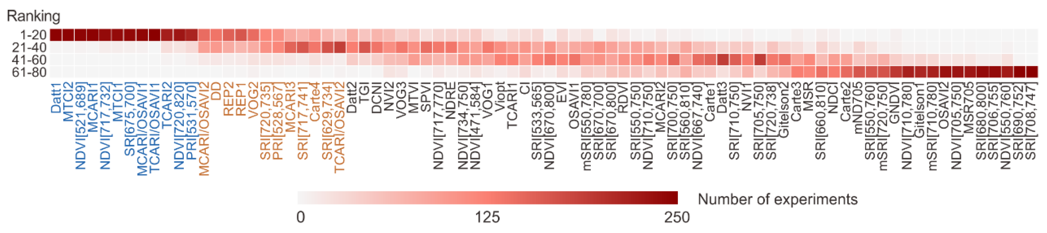
3.2. Feature Importance
3.3. Model Comparison and Performance
3.4. Model Adaptability for Different Compaction Treatments
4. Discussion
4.1. Selection of the Vegetation Indices
4.2. Advantages of the Ensemble Model
4.3. Effects of Machinery Compaction
5. Conclusions
Author Contributions
Funding
Acknowledgments
Conflicts of Interest
Appendix

| Feature | Model | R2 | RMSE (kg/ha) | MAE (kg/ha) |
|---|---|---|---|---|
| First derivatives of full bands | RF | 0.848 | 249.623 | 187.215 |
| SVR | 0.845 | 251.307 | 198.938 | |
| KNN | 0.823 | 267.859 | 210.981 | |
| Ensemble | 0.869 | 231.887 | 180.150 | |
| Second derivatives of full bands | RF | 0.820 | 270.324 | 209.001 |
| SVR | 0.814 | 275.077 | 217.356 | |
| KNN | 0.800 | 283.308 | 217.900 | |
| Ensemble | 0.836 | 258.841 | 201.951 | |
| First and second derivatives of full bands | RF | 0.856 | 241.011 | 181.244 |
| SVR | 0.854 | 243.162 | 195.826 | |
| KNN | 0.803 | 281.108 | 217.741 | |
| Ensemble | 0.874 | 226.434 | 177.255 | |
| Selected VIs | RF | 0.833 | 252.912 | 185.317 |
| SVR | 0.842 | 247.593 | 185.869 | |
| KNN | 0.850 | 241.430 | 183.557 | |
| Ensemble | 0.874 | 220.799 | 164.787 |
References
- Radović, J.; Sokolović, D.; Marković, J. Alfalfa-most important perennial forage legume in animal husbandry. Biotechnol. Anim. Husb. 2009, 25, 465–475. [Google Scholar] [CrossRef]
- United States Department of Agriculture National Agricultural Statistics Service. Available online: https://www.nass.usda.gov/ (accessed on 3 March 2020).
- Andrzejewska, J.; Contreras-Govea, F.E.; Albrecht, K.A. Field prediction of alfalfa (Medicago sativa L.) fibre constituents in northern Europe. Grass Forage Sci. 2014, 69, 348–355. [Google Scholar] [CrossRef]
- Noland, R.L.; Wells, M.S.; Coulter, J.A.; Tiede, T.; Baker, J.M.; Martinson, K.L.; Sheaffer, C.C. Estimating alfalfa yield and nutritive value using remote sensing and air temperature. Field Crops Res. 2018, 222, 189–196. [Google Scholar] [CrossRef]
- Summers, C.G.; Putnam, D.H. Irrigated Alfalfa Management for Mediterranean and Desert Zones; UCANR Publications: Davis, CA, USA, 2008; Volume 3512. [Google Scholar]
- Gląb, T. Effect of Soil Compaction on Root System Morphology and Productivity of Alfalfa (Medicago sativa L.). Pol. J. Environ. Stud. 2011, 20, 1473–1480. [Google Scholar]
- Harris, P.A.; Ellis, A.D.; Fradinho, M.J.; Jansson, A.; Julliand, V.; Luthersson, N.; Santos, A.S.; Vervuert, I. Feeding conserved forage to horses: Recent advances and recommendations. Animal 2017, 11, 958–967. [Google Scholar] [CrossRef] [Green Version]
- Manyawu, G. Principles of Silage Making; International Livestock Research Institute (ILRI): Nairobi, Kenya, 2016. [Google Scholar]
- Undersander, D.; Cosgrove, D. Alfalfa Management Guide; American Society of Agronomy Crop Science Society of America Soil Science: Madison, WI, USA, 2011. [Google Scholar]
- Schmierer, J.; Putnam, D.; Undersander, D.; Liu, J.; Meister, H. Wheel Traffic in Alfalfa–What do We Know? What Can We Do About It? In Proceedings of the National Alfalfa Symposium, San Diego, CA, USA, 13–15 December 2004; pp. 13–15. [Google Scholar]
- Rechel, E.A.; Meek, B.D.; DeTar, W.R.; Carter, L.M. Alfalfa yield as affected by harvest traffic and soil compaction in a sandy loam soil. J. Prod. Agric. 1991, 4, 241–246. [Google Scholar] [CrossRef]
- Undersander, D.; Moutray, J. Effect of Wheel Traffic on Alfalfa Yield. Available online: https://fyi.extension.wisc.edu/forage/effect-of-wheel-traffic-on-alfalfa/ (accessed on 3 March 2020).
- Orloff, S.; Putnam, D. Adjusting alfalfa cutting schedules for economic conditions. In Proceedings of the 40th California Alfalfa & Forage and Corn/Cereal Silage Mini-Symposium, Visalia, CA, USA, 1 December 2010; pp. 1–2. [Google Scholar]
- Undersander, D. Alfalfa Yield and Stand. Available online: https://fyi.extension.wisc.edu/forage/alfalfa-yield-and-stand/ (accessed on 3 March 2020).
- Daughtry, C.S.T.; Walthall, C.L.; Kim, M.S.; De Colstoun, E.B.; McMurtrey Iii, J.E. Estimating corn leaf chlorophyll concentration from leaf and canopy reflectance. Remote Sens. Environ. 2000, 74, 229–239. [Google Scholar] [CrossRef]
- Geipel, J.; Link, J.; Claupein, W. Combined spectral and spatial modeling of corn yield based on aerial images and crop surface models acquired with an unmanned aircraft system. Remote Sens. 2014, 6, 10335–10355. [Google Scholar] [CrossRef] [Green Version]
- Lauer, J. Methods for Calculating Corn Yield. 2002, Volume 33. Available online: http://corn.agronomy.wisc.edu/AA/A033.aspx (accessed on 3 March 2020).
- Ma, Y.; Kang, Y.; Ozdogan, M.; Zhang, Z. County-level corn yield prediction using deep transfer learning. AGUFM 2019, 2019, B54D-02. [Google Scholar]
- Wang, Y.; Zhang, Z.; Feng, L.; Du, Q.; Runge, T. Combining Multi-Source Data and Machine Learning Approaches to Predict Winter Wheat Yield in the Conterminous United States. Remote Sens. 2020, 12, 1232. [Google Scholar] [CrossRef] [Green Version]
- Pan, G.; Sun, G.-J.; Li, F.-M. Using QuickBird imagery and a production efficiency model to improve crop yield estimation in the semi-arid hilly Loess Plateau, China. Environ. Model. Softw. 2009, 24, 510–516. [Google Scholar] [CrossRef]
- Wahab, I.; Hall, O.; Jirström, M. Remote Sensing of Yields: Application of UAV Imagery-Derived NDVI for Estimating Maize Vigor and Yields in Complex Farming Systems in Sub-Saharan Africa. Drones 2018, 2, 28. [Google Scholar] [CrossRef] [Green Version]
- Su, W.; Zhang, M.; Bian, D.; Liu, Z.; Huang, J.; Wang, W.; Wu, J.; Guo, H. Phenotyping of Corn Plants Using Unmanned Aerial Vehicle (UAV) Images. Remote Sens. 2019, 11, 2021. [Google Scholar] [CrossRef] [Green Version]
- Kayad, A.G.; Al-Gaadi, K.A.; Tola, E.; Madugundu, R.; Zeyada, A.M.; Kalaitzidis, C. Assessing the spatial variability of alfalfa yield using satellite imagery and ground-based data. PLoS ONE 2016, 11, e0157166. [Google Scholar] [CrossRef]
- Sanches, G.M.; Duft, D.G.; Kölln, O.T.; Luciano, A.C.d.S.; De Castro, S.G.Q.; Okuno, F.M.; Franco, H.C.J. The potential for RGB images obtained using unmanned aerial vehicle to assess and predict yield in sugarcane fields. Int. J. Remote Sens. 2018, 39, 5402–5414. [Google Scholar] [CrossRef]
- Yun, H.S.; Park, S.H.; Kim, H.-J.; Lee, W.D.; Lee, K.D.; Hong, S.Y.; Jung, G.H. Use of unmanned aerial vehicle for multi-temporal monitoring of soybean vegetation fraction. J. Biosyst. Eng. 2016, 41, 126–137. [Google Scholar] [CrossRef] [Green Version]
- Zhou, X.; Zheng, H.B.; Xu, X.Q.; He, J.Y.; Ge, X.K.; Yao, X.; Cheng, T.; Zhu, Y.; Cao, W.X.; Tian, Y.C. Predicting grain yield in rice using multi-temporal vegetation indices from UAV-based multispectral and digital imagery. ISPRS J. Photogramm. Remote Sens. 2017, 130, 246–255. [Google Scholar] [CrossRef]
- Hassan, M.; Yang, M.; Rasheed, A.; Jin, X.; Xia, X.; Xiao, Y.; He, Z. Time-series multispectral indices from unmanned aerial vehicle imagery reveal senescence rate in bread wheat. Remote Sens. 2018, 10, 809. [Google Scholar] [CrossRef] [Green Version]
- Romero, M.; Luo, Y.; Su, B.; Fuentes, S. Vineyard water status estimation using multispectral imagery from an UAV platform and machine learning algorithms for irrigation scheduling management. Comput. Electron. Agric. 2018, 147, 109–117. [Google Scholar] [CrossRef]
- Maresma, Á.; Ariza, M.; Martínez, E.; Lloveras, J.; Martínez-Casasnovas, J. Analysis of vegetation indices to determine nitrogen application and yield prediction in maize (Zea mays L.) from a standard UAV service. Remote Sens. 2016, 8, 973. [Google Scholar] [CrossRef] [Green Version]
- Cárdenas, D.A.G.; Valencia, J.A.R.; Velásquez, D.F.A.; Gonzalez, J.R.P. Dynamics of the Indices NDVI and GNDVI in a Rice Growing in Its Reproduction Phase from Multi-spectral Aerial Images Taken by Drones. In Advances in Intelligent Systems and Computing, Proceedings of the 2nd International Conference of ICT for Adapting Agriculture to Climate Change (AACC’18), Cali, Colombia, 21–23 November 2018; Springer: Cham, Switzerland, 2018; pp. 106–119. [Google Scholar]
- Shen, X.; Cao, L.; Yang, B.; Xu, Z.; Wang, G. Estimation of forest structural attributes using spectral indices and point clouds from UAS-based multispectral and RGB imageries. Remote Sens. 2019, 11, 800. [Google Scholar] [CrossRef] [Green Version]
- Nidamanuri, R.R.; Zbell, B. Use of field reflectance data for crop mapping using airborne hyperspectral image. ISPRS J. Photogramm. Remote Sens. 2011, 66, 683–691. [Google Scholar] [CrossRef]
- Yang, C.; Everitt, J.H.; Bradford, J.M. Airborne hyperspectral imagery and linear spectral unmixing for mapping variation in crop yield. Precis. Agric. 2007, 8, 279–296. [Google Scholar] [CrossRef]
- Mewes, T.; Franke, J.; Menz, G. Spectral requirements on airborne hyperspectral remote sensing data for wheat disease detection. Precis. Agric. 2011, 12, 795. [Google Scholar] [CrossRef]
- Ray, S.S.; Jain, N.; Arora, R.K.; Chavan, S.; Panigrahy, S. Utility of hyperspectral data for potato late blight disease detection. J. Indian Soc. Remote Sens. 2011, 39, 161. [Google Scholar] [CrossRef]
- Kim, Y.; Glenn, D.M.; Park, J.; Ngugi, H.K.; Lehman, B.L. Hyperspectral image analysis for water stress detection of apple trees. Comput. Electron. Agric. 2011, 77, 155–160. [Google Scholar] [CrossRef]
- Ranjan, R.; Chopra, U.K.; Sahoo, R.N.; Singh, A.K.; Pradhan, S. Assessment of plant nitrogen stress in wheat (Triticum aestivum L.) through hyperspectral indices. Int. J. Remote Sens. 2012, 33, 6342–6360. [Google Scholar] [CrossRef]
- Jin, X.; Kumar, L.; Li, Z.; Xu, X.; Yang, G.; Wang, J. Estimation of winter wheat biomass and yield by combining the AquaCrop model and field hyperspectral data. Remote Sens. 2016, 8, 972. [Google Scholar] [CrossRef] [Green Version]
- Montesinos-López, O.A.; Montesinos-López, A.; Crossa, J.; de los Campos, G.; Alvarado, G.; Suchismita, M.; Rutkoski, J.; González-Pérez, L.; Burgueño, J. Predicting grain yield using canopy hyperspectral reflectance in wheat breeding data. Plant Methods 2017, 13, 4. [Google Scholar]
- Aguate, F.M.; Trachsel, S.; Pérez, L.G.; Burgueño, J.; Crossa, J.; Balzarini, M.; Gouache, D.; Bogard, M.; Campos, G.D.L. Use of hyperspectral image data outperforms vegetation indices in prediction of maize yield. Crop Sci. 2017, 57, 2517–2524. [Google Scholar] [CrossRef] [Green Version]
- Kawamura, K.; Ikeura, H.; Phongchanmaixay, S.; Khanthavong, P. Canopy hyperspectral sensing of paddy fields at the booting stage and PLS regression can assess grain yield. Remote Sens. 2018, 10, 1249. [Google Scholar] [CrossRef] [Green Version]
- Yang, C.; Everitt, J.H.; Bradford, J.M.; Murden, D. Comparison of airborne multispectral and hyperspectral imagery for estimating grain sorghum yield. Trans. ASABE 2009, 52, 641–649. [Google Scholar] [CrossRef]
- Oehlschläger, J.; Schmidhalter, U.; Noack, P.O. UAV-Based Hyperspectral Sensing for Yield Prediction in Winter Barley. In Proceedings of the 2018 9th Workshop on Hyperspectral Image and Signal Processing: Evolution in Remote Sensing (WHISPERS), Amsterdam, The Netherlands, 23–26 September 2018; pp. 1–4. [Google Scholar]
- Kanning, M.; Kühling, I.; Trautz, D.; Jarmer, T. High-resolution UAV-based hyperspectral imagery for LAI and chlorophyll estimations from wheat for yield prediction. Remote Sens. 2018, 10, 2000. [Google Scholar] [CrossRef] [Green Version]
- Moghimi, A.; Yang, C.; Anderson, J.A. Aerial hyperspectral imagery and deep neural networks for high-throughput yield phenotyping in wheat. arXiv 2019, arXiv:1906.09666. [Google Scholar]
- Zhao, J.; Karimzadeh, M.; Masjedi, A.; Wang, T.; Zhang, X.; Crawford, M.M.; Ebert, D.S. FeatureExplorer: Interactive Feature Selection and Exploration of Regression Models for Hyperspectral Images. In Proceedings of the 2019 IEEE Visualization Conference (VIS), Vancouver, BC, Canada, 20–25 October 2019; pp. 161–165. [Google Scholar]
- Schreiber, M.M.; Miles, G.E.; Holt, D.A.; Bula, R.J. Sensitivity Analysis of SIMED 1. Agron. J. 1978, 70, 105–108. [Google Scholar] [CrossRef]
- Fick, G.W. ALSIM 1 (Level 2) User’s Manual; Department of Agronomy, Cornell University: Ithaca, NY, USA, 1981. [Google Scholar]
- Denison, R.F.; Loomis, R.S. An Integrative Physiological Model of Alfalfa Growth and Development; Publication/University of California, Division of Agriculture and Natural Resources (USA): Davis, CA, USA, 1989. [Google Scholar]
- Bourgeois, G.; Savoie, P.; Girard, J.-M. Evaluation of an alfalfa growth simulation model under Quebec conditions. Agric. Syst. 1990, 32, 1–12. [Google Scholar] [CrossRef]
- Malik, W.; Boote, K.J.; Hoogenboom, G.; Cavero, J.; Dechmi, F. Adapting the CROPGRO model to simulate alfalfa growth and yield. Agron. J. 2018, 110, 1777–1790. [Google Scholar] [CrossRef] [Green Version]
- Cai, Y.; Moore, K.; Pellegrini, A.; Elhaddad, A.; Lessel, J.; Townsend, C.; Solak, H.; Semret, N. Crop yield predictions-high resolution statistical model for intra-season forecasts applied to corn in the US. In Proceedings of the American Geophysical Union 2017 Fall Meeting, New Orleans, LA, USA, 13 December 2017. [Google Scholar]
- Zhang, Z.; Jin, Y.; Chen, B.; Brown, P. California Almond Yield Prediction at the Orchard Level With a Machine Learning Approach. Front. Plant Sci. 2019, 10, 809. [Google Scholar] [CrossRef] [Green Version]
- Michel, L.; Makowski, D. Comparison of statistical models for analyzing wheat yield time series. PLoS ONE 2013, 8, e78615. [Google Scholar] [CrossRef] [Green Version]
- Gandhi, N.; Armstrong, L.J.; Petkar, O.; Tripathy, A.K. Rice crop yield prediction in India using support vector machines. In Proceedings of the 2016 13th International Joint Conference on Computer Science and Software Engineering (JCSSE), Khon Kaen, Thailand, 13–15 July 2016; pp. 1–5. [Google Scholar]
- Ali, I.; Cawkwell, F.; Green, S.; Dwyer, N. Application of statistical and machine learning models for grassland yield estimation based on a hypertemporal satellite remote sensing time series. In Proceedings of the 2014 IEEE Geoscience and Remote Sensing Symposium, Quebec City, QC, Canada, 13–18 July 2014; pp. 5060–5063. [Google Scholar]
- Pal, M. Ensemble learning with decision tree for remote sensing classification. World Acad. Sci. Eng. Technol. 2007, 36, 258–260. [Google Scholar]
- Zhang, Z.; Pasolli, E.; Crawford, M.M.; Tilton, J.C. An active learning framework for hyperspectral image classification using hierarchical segmentation. IEEE J. Sel. Top. Appl. Earth Obs. Remote Sens. 2015, 9, 640–654. [Google Scholar] [CrossRef]
- Zhang, Z.; Pasolli, E.; Crawford, M.M. An Adaptive Multiview Active Learning Approach for Spectral-Spatial Classification of Hyperspectral Images. IEEE Trans. Geosci. Remote Sens. 2019, 58, 2557–2570. [Google Scholar] [CrossRef]
- Zhou, Z.-H. Ensemble Learning. Encycl. Biom. 2009, 1, 270–273. [Google Scholar]
- Aghighi, H.; Azadbakht, M.; Ashourloo, D.; Shahrabi, H.S.; Radiom, S. Machine Learning Regression Techniques for the Silage Maize Yield Prediction Using Time-Series Images of Landsat 8 OLI. IEEE J. Sel. Top. Appl. Earth Obs. Remote Sens. 2018, 11, 4563–4577. [Google Scholar] [CrossRef]
- Feng, P.; Ma, J.; Sun, C.; Xu, X.; Ma, Y. A novel dynamic Android malware detection system with ensemble learning. IEEE Access 2018, 6, 30996–31011. [Google Scholar] [CrossRef]
- Ju, C.; Bibaut, A.; van der Laan, M. The relative performance of ensemble methods with deep convolutional neural networks for image classification. J. Appl. Stat. 2018, 45, 2800–2818. [Google Scholar] [CrossRef]
- U.S. Climate Data. Available online: https://www.usclimatedata.com/# (accessed on 3 March 2020).
- Habib, A.; Zhou, T.; Masjedi, A.; Zhang, Z.; Flatt, J.E.; Crawford, M. Boresight calibration of GNSS/INS-assisted push-broom hyperspectral scanners on UAV platforms. IEEE J. Sel. Top. Appl. Earth Obs. Remote Sens. 2018, 11, 1734–1749. [Google Scholar] [CrossRef]
- Peñuelas, J.; Filella, I. Visible and near-infrared reflectance techniques for diagnosing plant physiological status. Trends Plant Sci. 1998, 3, 151–156. [Google Scholar] [CrossRef]
- Thompson, W.M.O. The Whitefly, Bemisia Tabaci (Homoptera: Aleyrodidae) Interaction with Geminivirus-Infected Host Plants: Bemisia Tabaci, Host Plants and Geminiviruses; Springer Science & Business Media: Berlin/Heidelberg, Germany, 2011. [Google Scholar]
- Liang, L.; Di, L.; Zhang, L.; Deng, M.; Qin, Z.; Zhao, S.; Lin, H. Estimation of crop LAI using hyperspectral vegetation indices and a hybrid inversion method. Remote Sens. Environ. 2015, 165, 123–134. [Google Scholar] [CrossRef]
- Van Der Meij, B.; Kooistra, L.; Suomalainen, J.; Barel, J.M.; De Deyn, G.B. Remote sensing of plant trait responses to field-based plant-soil feedback using UAV-based optical sensors. Biogeosciences 2017, 14, 733. [Google Scholar] [CrossRef] [Green Version]
- Zhao, B.; Ma, B.L.; Hu, Y.; Liu, J. Characterization of nitrogen and water status in oat leaves using optical sensing approach. J. Sci. Food Agric. 2015, 95, 367–378. [Google Scholar] [CrossRef]
- Yu, K.; Gnyp, M.L.; Gao, J.; Miao, Y.; Chen, X.; Bareth, G. Using Partial Least Squares (PLS) to Estimate Canopy Nitrogen and Biomass of Paddy Rice in China’s Sanjiang Plain. In Proceedings of the Workshop on UAV-based Remote Sensing Methods for Monitoring Vegetation, Cologne, Germany, 14 April 2014; pp. 99–103. [Google Scholar]
- Tucker, C.J. Red and Photographic Infrared Linear Combinations for Monitoring Vegetation; NASA Goddard Space Flight Center: Greenbelt, MD, USA, 1978.
- Gitelson, A.; Merzlyak, M.N. Quantitative estimation of chlorophyll-ausing reflectance spectra: Experiments with autumn chestnut and maple leaves. J. Photochem. Photobiol. B Biol. 1994, 22, 247–252. [Google Scholar] [CrossRef]
- Wu, C.; Niu, Z.; Tang, Q.; Huang, W.; Rivard, B.; Feng, J. Remote estimation of gross primary production in wheat using chlorophyll-related vegetation indices. Agric. For. Meteorol. 2009, 149, 1015–1021. [Google Scholar] [CrossRef]
- Kooistra, L.; Suomalainen, J.; Iqbal, S.; Franke, J.; Wenting, P.; Bartholomeus, H.; Mücher, S.; Becker, R. Crop monitoring using a light-weight hyperspectral mapping system for unmanned aerial vehicles: First results for the 2013 season. In Proceedings of the Proceedings of 2013 Workshop on UAV-Based Remote Sensing Methods for Monitoring Vegetation, Cologne, Germany, 9–10 September 2013; p. 5158. [Google Scholar]
- Mutanga, O.; Skidmore, A.K. Narrow band vegetation indices overcome the saturation problem in biomass estimation. Int. J. Remote Sens. 2004, 25, 3999–4014. [Google Scholar] [CrossRef]
- Thenkabail, P.S.; Smith, R.B.; De Pauw, E. Hyperspectral vegetation indices and their relationships with agricultural crop characteristics. Remote Sens. Environ. 2000, 71, 158–182. [Google Scholar] [CrossRef]
- Gamon, J.A.; Penuelas, J.; Field, C.B. A narrow-waveband spectral index that tracks diurnal changes in photosynthetic efficiency. Remote Sens. Environ. 1992, 41, 35–44. [Google Scholar] [CrossRef]
- Penuelas, J.; Baret, F.; Filella, I. Semi-empirical indices to assess carotenoids/chlorophyll a ratio from leaf spectral reflectance. Photosynthetica 1995, 31, 221–230. [Google Scholar]
- Rodriguez, D.; Fitzgerald, G.J.; Belford, R.; Christensen, L.K. Detection of nitrogen deficiency in wheat from spectral reflectance indices and basic crop eco-physiological concepts. Aust. J. Agric. Res. 2006, 57, 781–789. [Google Scholar] [CrossRef] [Green Version]
- Sims, D.A.; Gamon, J.A. Relationships between leaf pigment content and spectral reflectance across a wide range of species, leaf structures and developmental stages. Remote Sens. Environ. 2002, 81, 337–354. [Google Scholar] [CrossRef]
- Gitelson, A.A.; Kaufman, Y.J.; Merzlyak, M.N. Use of a green channel in remote sensing of global vegetation from EOS-MODIS. Remote Sens. Environ. 1996, 58, 289–298. [Google Scholar] [CrossRef]
- Roujean, J.-L.; Breon, F.-M. Estimating PAR absorbed by vegetation from bidirectional reflectance measurements. Remote Sens. Environ. 1995, 51, 375–384. [Google Scholar] [CrossRef]
- Marshak, A.; Knyazikhin, Y.; Davis, A.B.; Wiscombe, W.J.; Pilewskie, P. Cloud-vegetation interaction: Use of normalized difference cloud index for estimation of cloud optical thickness. Geophys. Res. Lett. 2000, 27, 1695–1698. [Google Scholar] [CrossRef] [Green Version]
- Zarco-Tejada, P.J.; Pushnik, J.C.; Dobrowski, S.; Ustin, S.L. Steady-state chlorophyll a fluorescence detection from canopy derivative reflectance and double-peak red-edge effects. Remote Sens. Environ. 2003, 84, 283–294. [Google Scholar] [CrossRef]
- Datt, B. A new reflectance index for remote sensing of chlorophyll content in higher plants: Tests using Eucalyptus leaves. J. Plant Physiol. 1999, 154, 30–36. [Google Scholar] [CrossRef]
- Le Maire, G.; Francois, C.; Dufrene, E. Towards universal broad leaf chlorophyll indices using PROSPECT simulated database and hyperspectral reflectance measurements. Remote Sens. Environ. 2004, 89, 1–28. [Google Scholar] [CrossRef]
- Chen, P.; Haboudane, D.; Tremblay, N.; Wang, J.; Vigneault, P.; Li, B. New spectral indicator assessing the efficiency of crop nitrogen treatment in corn and wheat. Remote Sens. Environ. 2010, 114, 1987–1997. [Google Scholar] [CrossRef]
- Gitelson, A.A.; Buschmann, C.; Lichtenthaler, H.K. The chlorophyll fluorescence ratio F735/F700 as an accurate measure of the chlorophyll content in plants. Remote Sens. Environ. 1999, 69, 296–302. [Google Scholar] [CrossRef]
- Gitelson, A.A.; Gritz, Y.; Merzlyak, M.N. Relationships between leaf chlorophyll content and spectral reflectance and algorithms for non-destructive chlorophyll assessment in higher plant leaves. J. Plant Physiol. 2003, 160, 271–282. [Google Scholar] [CrossRef]
- Carter, G.A. Ratios of leaf reflectances in narrow wavebands as indicators of plant stress. Remote Sens. 1994, 15, 697–703. [Google Scholar] [CrossRef]
- Tian, Y.C.; Yao, X.; Yang, J.; Cao, W.X.; Hannaway, D.B.; Zhu, Y. Assessing newly developed and published vegetation indices for estimating rice leaf nitrogen concentration with ground-and space-based hyperspectral reflectance. Field Crops Res. 2011, 120, 299–310. [Google Scholar] [CrossRef]
- Gitelson, A.A.; Merzlyak, M.N. Remote estimation of chlorophyll content in higher plant leaves. Int. J. Remote Sens. 1997, 18, 2691–2697. [Google Scholar] [CrossRef]
- Xue, L.; Cao, W.; Luo, W.; Dai, T.; Zhu, Y. Monitoring leaf nitrogen status in rice with canopy spectral reflectance. Agron. J. 2004, 96, 135–142. [Google Scholar] [CrossRef]
- Zhu, Y.; Yao, X.; Tian, Y.; Liu, X.; Cao, W. Analysis of common canopy vegetation indices for indicating leaf nitrogen accumulations in wheat and rice. Int. J. Appl. Earth Obs. Geoinf. 2008, 10, 1–10. [Google Scholar] [CrossRef]
- McMurtrey Iii, J.E.; Chappelle, E.W.; Kim, M.S.; Meisinger, J.J.; Corp, L.A. Distinguishing nitrogen fertilization levels in field corn (Zea mays L.) with actively induced fluorescence and passive reflectance measurements. Remote Sens. Environ. 1994, 47, 36–44. [Google Scholar] [CrossRef]
- Chappelle, E.W.; Kim, M.S.; McMurtrey Iii, J.E. Ratio analysis of reflectance spectra (RARS): An algorithm for the remote estimation of the concentrations of chlorophyll a, chlorophyll b, and carotenoids in soybean leaves. Remote Sens. Environ. 1992, 39, 239–247. [Google Scholar] [CrossRef]
- Gupta, R.K.; Vijayan, D.; Prasad, T.S. Comparative analysis of red-edge hyperspectral indices. Adv. Space Res. 2003, 32, 2217–2222. [Google Scholar] [CrossRef]
- Zarco-Tejada, P.J.; Miller, J.R. Land cover mapping at BOREAS using red edge spectral parameters from CASI imagery. J. Geophys. Res. Atmos. 1999, 104, 27921–27933. [Google Scholar] [CrossRef]
- Gitelson, A.A.; Vina, A.; Ciganda, V.; Rundquist, D.C.; Arkebauer, T.J. Remote estimation of canopy chlorophyll content in crops. Geophys. Res. Lett. 2005, 32. [Google Scholar] [CrossRef] [Green Version]
- Gitelson, A.A.; Viña, A.; Arkebauer, T.J.; Rundquist, D.C.; Keydan, G.; Leavitt, B. Remote estimation of leaf area index and green leaf biomass in maize canopies. Geophys. Res. Lett. 2003, 30. [Google Scholar] [CrossRef] [Green Version]
- Chen, J.M. Evaluation of vegetation indices and a modified simple ratio for boreal applications. Can. J. Remote Sens. 1996, 22, 229–242. [Google Scholar] [CrossRef]
- Gupta, R.K.; Vijayan, D.; Prasad, T.S. New hyperspectral vegetation characterization parameters. Adv. Space Res. 2001, 28, 201–206. [Google Scholar] [CrossRef]
- Huete, A.; Justice, C.; Liu, H. Development of vegetation and soil indices for MODIS-EOS. Remote Sens. Environ. 1994, 49, 224–234. [Google Scholar] [CrossRef]
- Haboudane, D.; Miller, J.R.; Tremblay, N.; Zarco-Tejada, P.J.; Dextraze, L. Integrated narrow-band vegetation indices for prediction of crop chlorophyll content for application to precision agriculture. Remote Sens. Environ. 2002, 81, 416–426. [Google Scholar] [CrossRef]
- Wu, C.; Niu, Z.; Tang, Q.; Huang, W. Estimating chlorophyll content from hyperspectral vegetation indices: Modeling and validation. Agric. For. Meteorol. 2008, 148, 1230–1241. [Google Scholar] [CrossRef]
- Rondeaux, G.; Steven, M.; Baret, F. Optimization of soil-adjusted vegetation indices. Remote Sens. Environ. 1996, 55, 95–107. [Google Scholar] [CrossRef]
- Hunt, E.R., Jr.; Doraiswamy, P.C.; McMurtrey, J.E.; Daughtry, C.S.T.; Perry, E.M.; Akhmedov, B. A visible band index for remote sensing leaf chlorophyll content at the canopy scale. Int. J. Appl. Earth Obs. Geoinf. 2013, 21, 103–112. [Google Scholar] [CrossRef] [Green Version]
- Haboudane, D.; Miller, J.R.; Pattey, E.; Zarco-Tejada, P.J.; Strachan, I.B. Hyperspectral vegetation indices and novel algorithms for predicting green LAI of crop canopies: Modeling and validation in the context of precision agriculture. Remote Sens. Environ. 2004, 90, 337–352. [Google Scholar] [CrossRef]
- Dash, J.; Curran, P.J. The MERIS terrestrial chlorophyll index. Int. J. Remote Sens. 2004, 25, 5403–5413. [Google Scholar] [CrossRef]
- Main, R.; Cho, M.A.; Mathieu, R.; O’Kennedy, M.M.; Ramoelo, A.; Koch, S. An investigation into robust spectral indices for leaf chlorophyll estimation. ISPRS J. Photogramm. Remote Sens. 2011, 66, 751–761. [Google Scholar] [CrossRef]
- Guyot, G.; Baret, F. Utilisation de la haute resolution spectrale pour suivre l’etat des couverts vegetaux. In Proceedings of the Spectral Signatures of Objects in Remote Sensing, Aussois (Modane), France, 18–22 January 1988; p. 279. [Google Scholar]
- Vogelmann, J.E.; Rock, B.N.; Moss, D.M. Red edge spectral measurements from sugar maple leaves. TitleREMOTE Sens. 1993, 14, 1563–1575. [Google Scholar] [CrossRef]
- Reyniers, M.; Walvoort, D.J.J.; De Baardemaaker, J. A linear model to predict with a multi-spectral radiometer the amount of nitrogen in winter wheat. Int. J. Remote Sens. 2006, 27, 4159–4179. [Google Scholar] [CrossRef]
- Moghimi, A.; Yang, C.; Marchetto, P.M. Ensemble feature selection for plant phenotyping: A journey from hyperspectral to multispectral imaging. IEEE Access 2018, 6, 56870–56884. [Google Scholar] [CrossRef]
- Cai, J.; Luo, J.; Wang, S.; Yang, S. Feature selection in machine learning: A new perspective. Neurocomputing 2018, 300, 70–79. [Google Scholar] [CrossRef]
- Johannes, M.; Brase, J.C.; Fröhlich, H.; Gade, S.; Gehrmann, M.; Fälth, M.; Sültmann, H.; Beißbarth, T. Integration of pathway knowledge into a reweighted recursive feature elimination approach for risk stratification of cancer patients. Bioinformatics 2010, 26, 2136–2144. [Google Scholar] [CrossRef] [Green Version]
- Zhang, C.; Li, Y.; Yu, Z.; Tian, F. Feature selection of power system transient stability assessment based on random forest and recursive feature elimination. In Proceedings of the 2016 IEEE PES Asia-Pacific Power and Energy Engineering Conference (APPEEC), Xi’an, China, 25–28 October 2016; pp. 1264–1268. [Google Scholar]
- Feng, L.; Li, Y.; Wang, Y.; Du, Q. Estimating hourly and continuous ground-level PM2. 5 concentrations using an ensemble learning algorithm: The ST-stacking model. Atmos. Environ. 2020, 223, 117242. [Google Scholar] [CrossRef]
- González Sánchez, A.; Frausto Solís, J.; Ojeda Bustamante, W. Predictive ability of machine learning methods for massive crop yield prediction. SJAR 2014, 12, 313–328. [Google Scholar] [CrossRef] [Green Version]
- Jaikla, R.; Auephanwiriyakul, S.; Jintrawet, A. Rice yield prediction using a support vector regression method. In Proceedings of the 2008 5th International Conference on Electrical Engineering/Electronics, Computer, Telecommunications and Information Technology, Krabi, Thailand, 14–17 May 2008; pp. 29–32. [Google Scholar]
- Chlingaryan, A.; Sukkarieh, S.; Whelan, B. Machine learning approaches for crop yield prediction and nitrogen status estimation in precision agriculture: A review. Comput. Electron. Agric. 2018, 151, 61–69. [Google Scholar] [CrossRef]
- Awad, M.; Khanna, R. Support vector regression. In Efficient Learning Machines; Springer: Berlin/Heidelberg, Germany, 2015; pp. 67–80. [Google Scholar]
- Breiman, L. Random forests. Mach. Learn. 2001, 45, 5–32. [Google Scholar] [CrossRef] [Green Version]
- Zhou, X.; Zhu, X.; Dong, Z.; Guo, W. Estimation of biomass in wheat using random forest regression algorithm and remote sensing data. Crop J. 2016, 4, 212–219. [Google Scholar]
- Wang, Y.; Wu, X.; Chen, Z.; Ren, F.; Feng, L.; Du, Q. Optimizing the Predictive Ability of Machine Learning Methods for Landslide Susceptibility Mapping Using SMOTE for Lishui City in Zhejiang Province, China. Int. J. Environ. Res. Public Health 2019, 16, 368. [Google Scholar] [CrossRef] [Green Version]
- Yang, Q.; Shi, L.; Han, J.; Zha, Y.; Zhu, P. Deep convolutional neural networks for rice grain yield estimation at the ripening stage using UAV-based remotely sensed images. Field Crops Res. 2019, 235, 142–153. [Google Scholar] [CrossRef]
- Dayananda, S.; Astor, T.; Wijesingha, J.; Chickadibburahalli Thimappa, S.; Dimba Chowdappa, H.; Nidamanuri, R.R.; Nautiyal, S.; Wachendorf, M. Multi-Temporal Monsoon Crop Biomass Estimation Using Hyperspectral Imaging. Remote Sens. 2019, 11, 1771. [Google Scholar] [CrossRef] [Green Version]
- Wilkerson, S. Application of the Paired t-test. XULAneXUS 2008, 5, 7. [Google Scholar]
- Hansen, P.M.; Schjoerring, J.K. Reflectance measurement of canopy biomass and nitrogen status in wheat crops using normalized difference vegetation indices and partial least squares regression. Remote Sens. Environ. 2003, 86, 542–553. [Google Scholar] [CrossRef]
- Cazenave, A.-B.; Shah, K.; Trammell, T.; Komp, M.; Hoffman, J.; Motes, C.M.; Monteros, M.J. High-Throughput Approaches for Phenotyping Alfalfa Germplasm under Abiotic Stress in the Field. Plant Phenome J. 2019, 2, 1–13. [Google Scholar] [CrossRef]
- Cho, M.A.; Skidmore, A.; Corsi, F.; Van Wieren, S.E.; Sobhan, I. Estimation of green grass/herb biomass from airborne hyperspectral imagery using spectral indices and partial least squares regression. Int. J. Appl. Earth Obs. Geoinf. 2007, 9, 414–424. [Google Scholar] [CrossRef]
- Clevers, J.G.P.W. Imaging spectrometry in agriculture-plant vitality and yield indicators. In Imaging Spectrometry—A Tool for Environmental Observations; Springer: Berlin/Heidelberg, Germany, 1994; pp. 193–219. [Google Scholar]
- Gabriel, J.L.; Zarco-Tejada, P.J.; López-Herrera, P.J.; Pérez-Martín, E.; Alonso-Ayuso, M.; Quemada, M. Airborne and ground level sensors for monitoring nitrogen status in a maize crop. Biosyst. Eng. 2017, 160, 124–133. [Google Scholar] [CrossRef]
- Frame, J.; Merrilees, D.W. The effect of tractor wheel passes on herbage production from diploid and tetraploid ryegrass swards. Grass Forage Sci. 1996, 51, 13–20. [Google Scholar] [CrossRef]
- Meek, B.D.; Carter, L.M.; Garber, R.H.; Rechel, E.A.; DeTar, W.R.; Shatter, C.A. Regrowth and Yield of Alfalfa as Influenced by Wheel Traffic. Available online: http://works.bepress.com/william_detar/24/ (accessed on 3 March 2020).


| Treatment | Name | Simulated Traffic | Description |
|---|---|---|---|
| T1 | Single Pass Silage/Hay | Mower | One application of compaction immediately after harvest covering the entire plot. |
| T2 | Three Passes Silage | Mower, merger, forage harvester | Three applications of compaction. One immediately after harvest, one 24 h after harvest, and one 26 h after harvest. Full plot application. |
| T3 | Five Passes Silage | Mower, merger, rake, forage harvester, transport vehicle | Five applications of compaction. One immediately after harvest, two passes 24 h after harvest, and two passes 26 h after harvest. Full plot application. |
| T4 | Simulated Silage producer | Mower, merger or rake, forage harvester, transport vehicle | Two-wheel tracks applied within the plot. One pass immediately after harvest, one pass 24 h after harvest, and two passes 26 h after harvest. |
| T5 | Three Passes Hay | Mower, merger or rake, bailer | Three applications of compaction. One immediately after harvest, one 48 h after harvest, and one 72 h after harvest. Full plot application. |
| T6 | Five Passes Hay | Mower, merger, rake, bailer, transport vehicle | Five applications of compaction. One immediately after harvest, two passes 48 h after harvest, and two passes 72 h after harvest. Full plot application. |
| T7 | Zero Passes | No | No machine traffic applied. |
| Full Form | Index | Formula | Reference |
|---|---|---|---|
| Normalized difference vegetation index | NDVI[471,584] | (R584 − R471)/(R584 + R471) | [69] |
| NDVI[521,689] | (R689 − R521)/(R689 + R521) | [69] | |
| NDVI[550,760] | (R760 − R550)/(R760 + R550) | [70] | |
| NDVI[667,740] | (R740 − R667)/(R740 + R667) | [71] | |
| NDVI[670,800] | (R800 − R670)/(R800 + R670) | [72] | |
| NDVI[705,750] | (R750 − R705)/(R750 + R705) | [73] | |
| NDVI[710,750] | (R750 − R710)/(R750 + R710) | [74] | |
| NDVI[710,780] | (R780 − R710)/(R780 + R710) | [75] | |
| NDVI[717,732] | (R750 − R710)/(R750 + R710) | [76] | |
| NDVI[717,770] | (R732 − R717)/(R732 + R717) | [76] | |
| NDVI[720,820] | (R820 − R720)/(R820 + R720) | [77] | |
| NDVI[734,750] | (R750 − R735)/(R750 + R734) | [76] | |
| Physiological reflectance index | PRI[528,567] | (R528 − R567)/(R528 + R567) | [78] |
| PRI[531,570] | (R570 − R531)/(R531 + R570) | [79] | |
| Normalized difference red edge | NDRE | (R790 − R720)/(R790 + R720) | [80] |
| Modified normalized difference vegetation index | mND705 | (R750 − R705)/(R750 + R705 − 2R445) | [81] |
| Green normalized difference vegetation index | GNDVI | (R750 − R550)/(R750 + R550) | [82] |
| Renormalized difference vegetation index | RDVI | ) | [83] |
| Normalized difference cloud index | NDCI | (R762 − R527)/(R762 + R527) | [84] |
| Curvature index | CI | R675 × R690/R6832 | [85] |
| - | Datt1 | (R850 − R710)/(R850 − R680) | [86] |
| Datt2 | R850/R710 | ||
| Datt3 | R754/R704 | ||
| Double Difference index | DD | (R749 − R720) − (R701 − R672) | [87] |
| Double peak canopy nitrogen index | DCNI | (R720 − R700)/[(R700 − R670)(R720 − R670 + 0.03)] | [88] |
| - | Gitelson1 | 1/R700 | [89] |
| Gitelson2 | (R750-R800/R695-R740) − 1 | [90] | |
| - | Carte1 | R695/R760 | [91] |
| Carte2 | R605/R760 | ||
| Carte3 | R710/R760 | ||
| Carte4 | R695/R670 | ||
| Simple ratio index | SRI[533,565] | R565/R533 | [92] |
| SRI[550,750] | R750/R550 | [93] | |
| SRI[550,760] | R760/R550 | [70] | |
| SRI[560,810] | R810/R560 | [94] | |
| SRI[629,734] | R734/R629 | [71] | |
| SRI[660,810] | R810/R660 | [95] | |
| SRI[670,700] | R700/R670 | [96] | |
| SRI[670,800] | R800/R670 | [88] | |
| SRI[675,700] | R675/R700 | [97] | |
| SRI[680,800] | R800/R680 | [81] | |
| SRI[690,752] | R752/R690 | [93] | |
| SRI[700,750] | R750/R700 | [93] | |
| SRI[705,750] | R750/R705 | [73] | |
| SRI[706,755] | R706/R755 | [76] | |
| SRI[708,747] | R747/R708 | [98] | |
| SRI[710,750] | R750/R710 | [99] | |
| SRI[717,741] | R741/R717 | [98] | |
| SRI[720,735] | R735/R720 | [98] | |
| SRI[720,738] | R738/R720 | [98] | |
| Modified simple ratio index | mSRI[550,780] | R780/R550-1 | [100] |
| mSRI[710,780] | R780/R710-1 | [101] | |
| mSRI[720,750] | R750/R720-1 | [100] | |
| mSR705 | (R750 − R445)/(R705 − R445) | [86] | |
| mSR | [102] | ||
| New vegetation index | NVI1 | (R777 − R747)/R673 | [103] |
| NVI2 | R705/(R717 + R491) | [92] | |
| Enhanced vegetation index | EVI | 2.5(R800 − R670)/(R800 − 6R670 − 7.5R475 + 1) | [104] |
| Transformed Chlorophyll absorption in reflectance index | TCARI1 | 3[(R700 − R670) − 0.2(R700 − R550)(R700/R670)] | [105] |
| TCARI2 | 3[(R750 − R705) − 0.2(R750 − R550)(R750/R705)] | [106] | |
| Modified chlorophyll absorption ratio index | MCARI1 | [(R700 − R670) − 0.2(R700 − R550)](R700/R670) | [15] |
| MCARI2 | [(R750 − R705) − 0.2(R750 − R550)](R750/R705) | [106] | |
| MCARI3 | [(R750 − R710) − 0.2(R750 − R550)](R750/R715) | [106] | |
| Optimized soil-adjusted vegetation index | OSAVI1 | (1 + 0.16)(R800 − R670)/(R800 + R670 + 0.16) | [107] |
| OSAVI2 | (1 + 0.16)(R750 − R705)/(R750 + R705 + 0.16) | [106] | |
| Combined TCARI/OSAVI | TCARI/OSAVI1 | TCARI1/OSAVI1 | [105] |
| TCARI/OSAVI2 | TCARI2/OSAVI2 | [106] | |
| Combined MCARI/OSAVI | MCARI/OSAVI1 | MCARI1/OSAVI1 | [106] |
| MCARI/OSAVI2 | MCARI2/OSAVI2 | [106] | |
| Triangular greenness index | TGI | −0.5[190(R670-R550) − 120(R670 − R480)] | [108] |
| Modified triangular vegetation index | MTVI | 1.2[1.2(R800 − R550) − 2.5(670 − R550)] | [109] |
| MERIS terrestrial chlorophyll index | MTCI1 | (R750 − R710)/(R710 − R680) | [110] |
| MTCI2 | (R754 − R709)/(R709 − R681) | ||
| Spectral polygon vegetation index | SPVI | 0.4 × [3.7(R800 − R670) − 1.2|R550 − R670|] | [111] |
| Red edge position index | REP1 | 700 + 45[(R670 + R780)/2 − R700]/(R740 − R700) | [69] |
| REP2 | 700 + 40[(R670 + R780)/2 − R700]/(R740 − R700) | [112] | |
| - | VOG1 | R740/R720 | [113] |
| VOG2 | (R734 − R747)/(R715 + R726) | ||
| VOG3 | (R734 − R747)/(R715 + R720) | ||
| Optimal vegetation index | Viopt | (1 + 0.45)(R8002 + 1)/(R670 + 0.45) | [114] |
| Harvesting Time | Treatment | Mean (kg/ha) | Max. (kg/ha) | Min. (kg/ha) | STD (kg/ha) |
|---|---|---|---|---|---|
| August | T1 | 2256.319 | 3170.609 | 1333.134 | 450.226 |
| T2 | 2172.798 | 2495.764 | 1066.013 | 383.013 | |
| T3 | 2074.944 | 2447.826 | 1282.724 | 324.696 | |
| T4 | 2150.558 | 2752.013 | 923.186 | 500.141 | |
| T5 | 2037.878 | 2729.032 | 1436.424 | 373.870 | |
| T6 | 1808.317 | 2453.262 | 1095.171 | 357.561 | |
| T7 | 2215.053 | 2686.530 | 1328.933 | 359.785 | |
| September | T1 | 1282.477 | 1528.347 | 1012.144 | 172.232 |
| T2 | 1077.874 | 1441.119 | 295.044 | 304.434 | |
| T3 | 951.109 | 1262.709 | 510.520 | 230.796 | |
| T4 | 1171.774 | 1475.466 | 386.226 | 284.171 | |
| T5 | 868.823 | 1182.646 | 678.304 | 170.256 | |
| T6 | 701.285 | 1049.704 | 256.495 | 228.078 | |
| T7 | 1241.705 | 1439.142 | 562.412 | 228.325 |
| Feature | Ranking | Feature | Ranking |
|---|---|---|---|
| Datt1 | 1 | SPVI | 41 |
| MCARI1 | 2 | mSRI[720,750] | 42 |
| MTCI2 | 3 | VOG1 | 43 |
| MCARI/OSAVI1 | 4 | Carte2 | 44 |
| MTCI1 | 5 | TCARI1 | 45 |
| REP2 | 6 | MCARI2 | 46 |
| PRI[531,570] | 7 | Carte1 | 47 |
| SR[675,700] | 8 | NVI1 | 48 |
| NDVI[521,689] | 9 | NDVI[471,584] | 49 |
| NDVI[717,732] | 10 | NDVI[667,740] | 50 |
| REP1 | 11 | Datt2 | 51 |
| TCARI/OSAVI1 | 12 | mSR | 52 |
| NVI2 | 13 | RDVI | 53 |
| TCARI2 | 14 | SRI[560,810] | 54 |
| TCARI/OSAVI2 | 15 | NDVI[710,750] | 55 |
| NDVI[720,820] | 16 | SRI[710,750] | 56 |
| Carte4 | 17 | Datt3 | 57 |
| NDVI[734,750] | 18 | mND705 | 58 |
| VOG3 | 19 | mSRI[710,780] | 59 |
| PRI[528,567] | 20 | Gitelson1 | 60 |
| VOG2 | 21 | OSAVI1 | 61 |
| NDRE | 22 | SRI[705,750] | 62 |
| SRI[533,565] | 23 | Gitelson2 | 63 |
| EVI | 24 | NDVI[717,770] | 64 |
| SRI[720,735] | 25 | SRI[670,800] | 65 |
| SRI[629,734] | 26 | NDCI | 66 |
| DD | 27 | Carte3 | 67 |
| MCARI/OSAVI2 | 28 | SRI[660,810] | 68 |
| CI | 29 | OSAVI2 | 69 |
| SRI[670,700] | 30 | mSRI[550,780] | 70 |
| MTVI | 31 | NDVI[705,750] | 71 |
| SRI[700,750] | 32 | NDVI[710,780] | 72 |
| NDVI[550,760] | 33 | SRI[550,750] | 73 |
| MCARI3 | 34 | SRI[706,755] | 74 |
| SRI[717,741] | 35 | SRI[550,760] | 75 |
| DCNI | 36 | SRI[708,747] | 76 |
| TGI | 37 | mSR705 | 77 |
| NDVI[670,800] | 38 | SRI[680,800] | 78 |
| SRI[720,738] | 39 | GNDVI | 79 |
| Viopt | 40 | SRI[690,752] | 80 |
| Feature | Model | R2 | RMSE (kg/ha) | MAE (kg/ha) |
|---|---|---|---|---|
| Selected features | RF | 0.833 | 252.912 | 185.317 |
| (0.052) | (36.243) | (27.611) | ||
| SVR | 0.842 | 247.593 | 185.869 | |
| (0.042) | (36.269) | (27.128) | ||
| KNN | 0.850 | 241.430 | 183.557 | |
| (0.035) | (31.183) | (25.998) | ||
| Ensemble | 0.874 | 220.799 | 164.787 | |
| (0.034) | (32.169) | (24.673) | ||
| Full features | RF | 0.822 | 261.552 | 191.602 |
| (0.054) | (35.718) | (28.109) | ||
| SVR | 0.829 | 257.408 | 191.590 | |
| (0.042) | (30.260) | (23.569) | ||
| KNN | 0.822 | 262.907 | 198.293 | |
| (0.044) | (35.417) | (28.847) | ||
| Ensemble | 0.854 | 237.906 | 175.575 | |
| (0.036) | (32.152) | (25.300) |
| Feature | Model | t | p-Value |
|---|---|---|---|
| Selected features | Ensemble vs. RF | 18.355 | 0.000 |
| Ensemble vs. SVR | 16.890 | 0.000 | |
| Ensemble vs. KNN | 17.059 | 0.000 | |
| Full features | Ensemble vs. RF | 15.935 | 0.000 |
| Ensemble vs. SVR | 13.957 | 0.000 | |
| Ensemble vs. KNN | 20.255 | 0.000 |
| Model | Metrics | T1 | T2 | T3 | T4 | T5 | T6 | T7 |
|---|---|---|---|---|---|---|---|---|
| RF | R2 | 0.863 | 0.852 | 0.908 | 0.762 | 0.880 | 0.731 | 0.759 |
| RMSE (kg/ha) | 221.319 | 249.490 | 190.915 | 310.648 | 226.252 | 327.119 | 281.774 | |
| MAE (kg/ha) | 170.618 | 192.834 | 132.685 | 216.692 | 154.630 | 229.184 | 196.870 | |
| SVR | R2 | 0.845 | 0.889 | 0.871 | 0.702 | 0.906 | 0.801 | 0.784 |
| RMSE (kg/ha) | 235.242 | 215.894 | 225.637 | 347.210 | 200.501 | 281.140 | 266.777 | |
| MAE (kg/ha) | 166.508 | 168.490 | 172.771 | 254.350 | 162.607 | 228.031 | 185.659 | |
| KNN | R2 | 0.851 | 0.831 | 0.900 | 0.850 | 0.891 | 0.774 | 0.745 |
| RMSE (kg/ha) | 230.624 | 266.081 | 198.819 | 246.571 | 216.394 | 299.885 | 289.737 | |
| MAE (kg/ha) | 185.806 | 222.928 | 151.893 | 172.299 | 166.075 | 240.781 | 210.967 | |
| Ensemble | R2 | 0.873 | 0.869 | 0.918 | 0.839 | 0.914 | 0.837 | 0.778 |
| RMSE (kg/ha) | 212.574 | 234.157 | 180.469 | 255.500 | 192.307 | 254.738 | 270.159 | |
| MAE (kg/ha) | 159.047 | 185.788 | 126.512 | 191.685 | 142.453 | 191.387 | 189.763 |
© 2020 by the authors. Licensee MDPI, Basel, Switzerland. This article is an open access article distributed under the terms and conditions of the Creative Commons Attribution (CC BY) license (http://creativecommons.org/licenses/by/4.0/).
Share and Cite
Feng, L.; Zhang, Z.; Ma, Y.; Du, Q.; Williams, P.; Drewry, J.; Luck, B. Alfalfa Yield Prediction Using UAV-Based Hyperspectral Imagery and Ensemble Learning. Remote Sens. 2020, 12, 2028. https://doi.org/10.3390/rs12122028
Feng L, Zhang Z, Ma Y, Du Q, Williams P, Drewry J, Luck B. Alfalfa Yield Prediction Using UAV-Based Hyperspectral Imagery and Ensemble Learning. Remote Sensing. 2020; 12(12):2028. https://doi.org/10.3390/rs12122028
Chicago/Turabian StyleFeng, Luwei, Zhou Zhang, Yuchi Ma, Qingyun Du, Parker Williams, Jessica Drewry, and Brian Luck. 2020. "Alfalfa Yield Prediction Using UAV-Based Hyperspectral Imagery and Ensemble Learning" Remote Sensing 12, no. 12: 2028. https://doi.org/10.3390/rs12122028
APA StyleFeng, L., Zhang, Z., Ma, Y., Du, Q., Williams, P., Drewry, J., & Luck, B. (2020). Alfalfa Yield Prediction Using UAV-Based Hyperspectral Imagery and Ensemble Learning. Remote Sensing, 12(12), 2028. https://doi.org/10.3390/rs12122028