Improved Ice Velocity Measurements with Sentinel-1 TOPS Interferometry

 , , and
Abstract
:
1. Introduction
2. Data and Methods
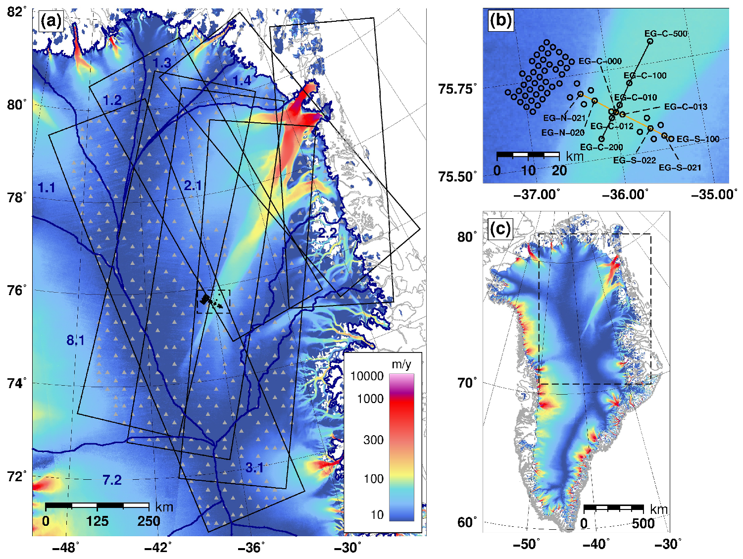
2.1. Data
2.2. Intensity Offset Tracking
2.3. Sentinel-1 TOPS Interferometry
2.3.1. Theoretical Background
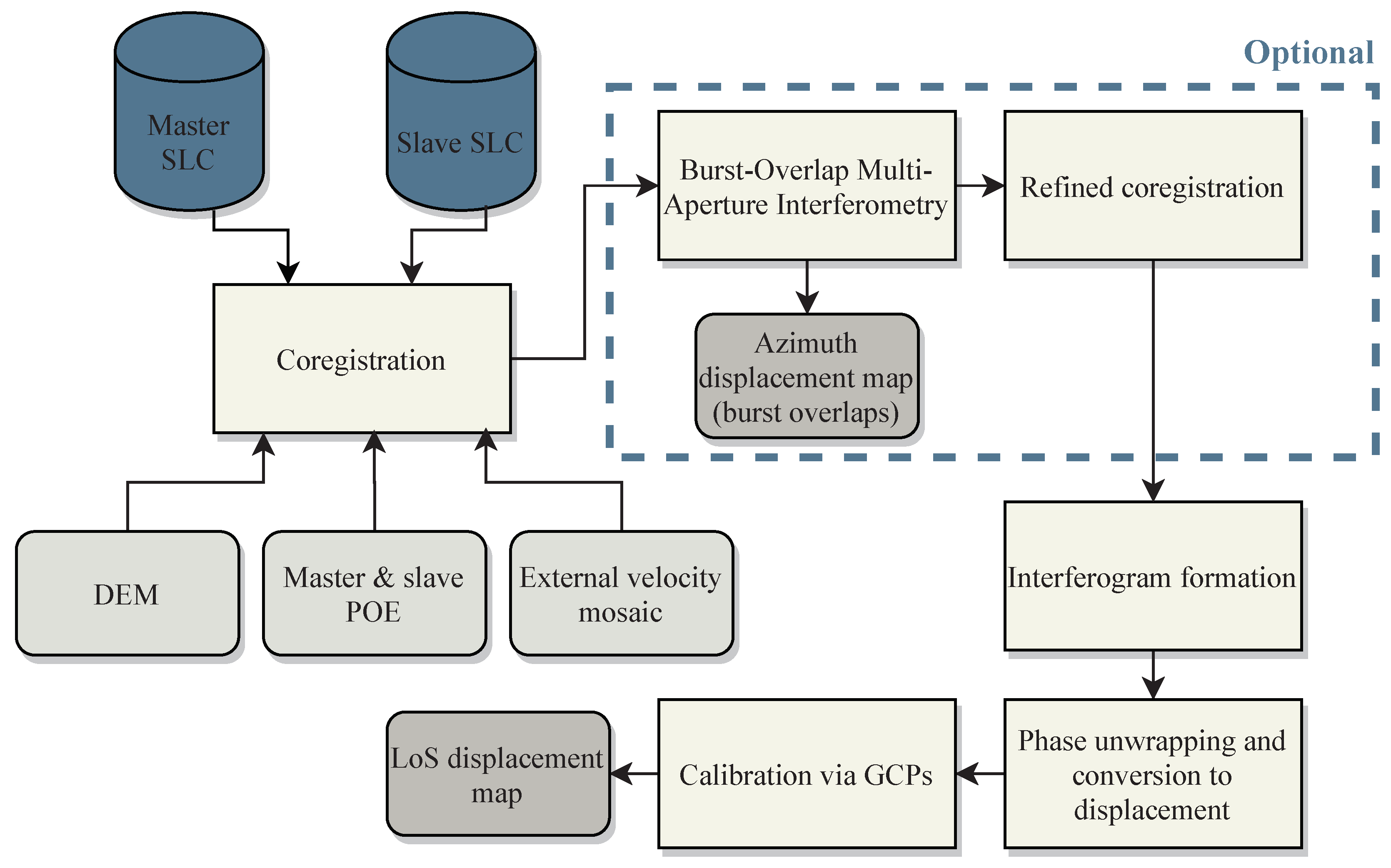
2.3.2. Processing Algorithm
2.4. Calibration and Error Estimation
2.5. Fusion of Velocity Measurements
3. Results
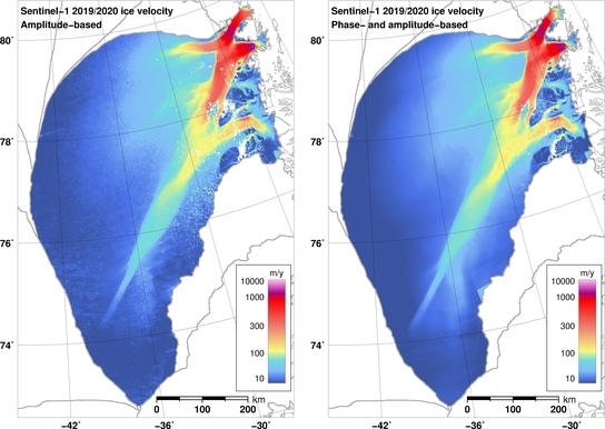
3.1. SAR-Based Ice Velocity Mosaics
3.2. Validation
4. Discussion
5. Conclusions
Supplementary Materials
Author Contributions
Funding
Acknowledgments
Conflicts of Interest
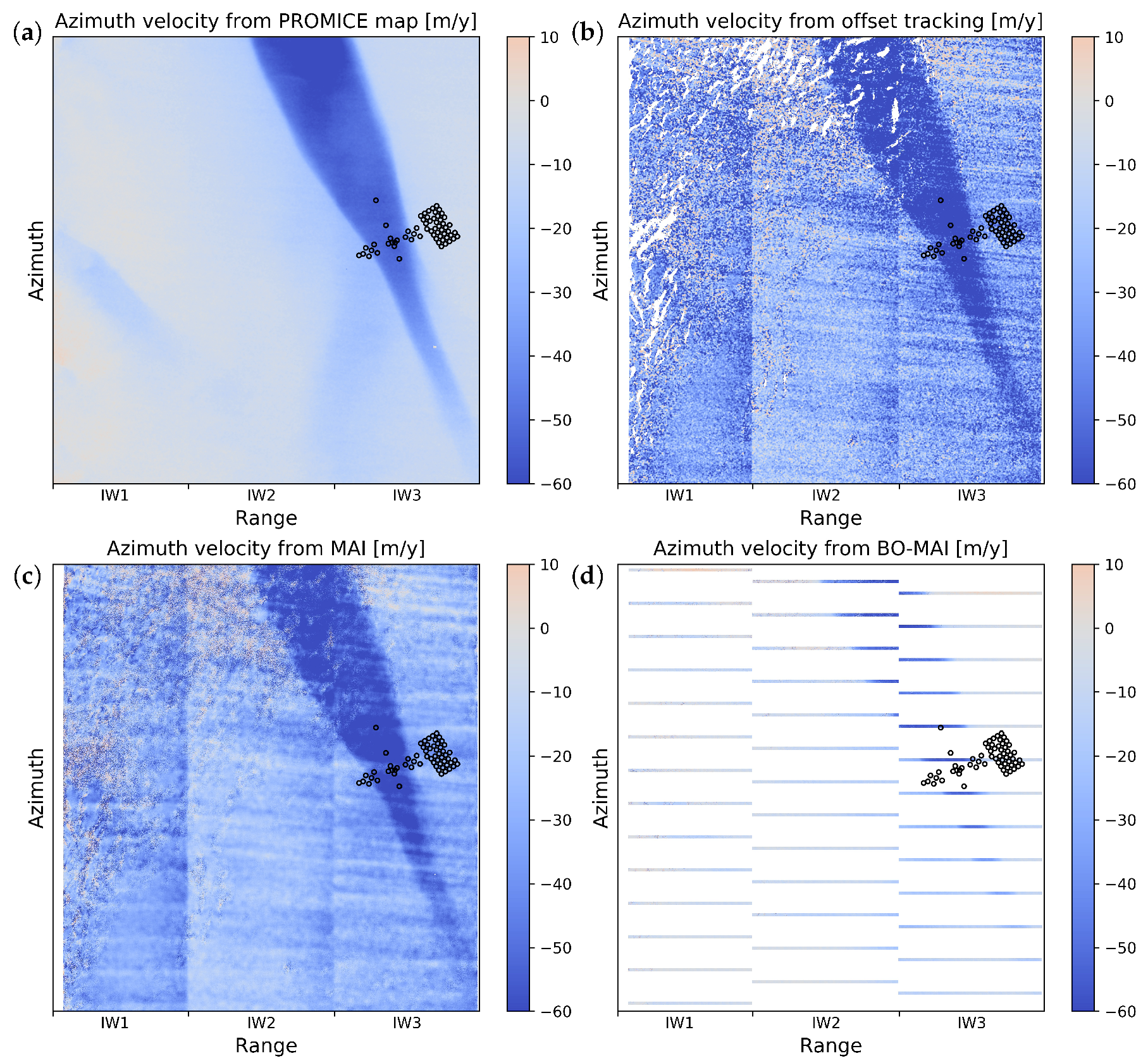
Appendix A. Azimuth Ice Velocity Measurements with Sentinel-1

| Method | Mean | Std. |
|---|---|---|
| PROMICE multi-year (offset tracking) | 0.91 | 0.72 |
| Azimuth offset tracking | −22.02 | 13.63 |
| Multi-Aperture Interferometry (MAI) | −18.24 | 8.92 |
| Burst-Overlap MAI (BO-MAI) | −0.79 | 1.10 |
| Mean | |||
|---|---|---|---|
| Method | IW1 | IW2 | IW3 |
| Offset tracking (6-day) | −29.94 | −16.80 | −19.65 |
| MAI (6-day) | −26.20 | −13.63 | −15.02 |
| BO-MAI (6-day) | −1.13 | 1.11 | 0.73 |
References
- Shepherd, A.; Ivins, E.; Rignot, E.; Smith, B.; van den Broeke, M.; Velicogna, I.; Whitehouse, P.; Briggs, K.; Joughin, I.; Krinner, G.; et al. Mass balance of the Greenland Ice Sheet from 1992 to 2018. Nature 2020, 579, 233–239. [Google Scholar] [CrossRef]
- Box, J.E.; Colgan, W.T.; Wouters, B.; Burgess, D.O.; O’Neel, S.; Thomson, L.I.; Mernild, S.H. Global sea-level contribution from Arctic land ice: 1971–2017. Environ. Res. Lett. 2018, 13, 125012. [Google Scholar] [CrossRef] [Green Version]
- Gray, A.; Mattar, K.; Vachon, P.; Bindschadler, R.; Jezek, K.; Forster, R.; Crawford, J. InSAR results from the RADARSAT Antarctic Mapping Mission data: Estimation of glacier motion using a simple registration procedure. In Proceedings of the IGARSS ’98. Sensing and Managing the Environment, 1998 IEEE International Geoscience and Remote Sensing (Cat. No.98CH36174), Seattle, WA, USA, 6–10 July 1998; Volume 3, pp. 1638–1640. [Google Scholar] [CrossRef]
- Strozzi, T.; Luckman, A.; Murray, T.; Wegmüller, U.; Werner, C.L. Glacier motion estimation using SAR offset-tracking procedures. IEEE Trans. Geosci. Remote Sens. 2002, 40, 2384–2391. [Google Scholar] [CrossRef] [Green Version]
- Goldstein, R.M.; Engelhardt, H.; Kamb, B.; Frolich, R.M. Satellite radar interferometry for monitoring ice sheet motion: Application to an Antarctic ice stream. Science 1993, 262, 1525–1530. [Google Scholar] [CrossRef]
- Merryman Boncori, J.P.; Langer Andersen, M.; Dall, J.; Kusk, A.; Kamstra, M.; Bech Andersen, S.; Bechor, N.; Bevan, S.; Bignami, C.; Gourmelen, N.; et al. Intercomparison and Validation of SAR-Based Ice Velocity Measurement Techniques within the Greenland Ice Sheet CCI Project. Remote Sens. 2018, 10, 929. [Google Scholar] [CrossRef] [Green Version]
- De Zan, F.; Guarnieri, A.M. TOPSAR: Terrain observation by progressive scans. IEEE Trans. Geosci. Remote Sens. 2006, 44, 2352–2360. [Google Scholar] [CrossRef]
- Nagler, T.; Rott, H.; Hetzenecker, M.; Wuite, J.; Potin, P. The Sentinel-1 mission: New opportunities for ice sheet observations. Remote Sens. 2015, 7, 9371–9389. [Google Scholar] [CrossRef] [Green Version]
- PROMICE Scientific Data Portal: Sentinel-1 Greenland Ice Velocity, produced by GEUS and DTU Space. Available online: http://www.promice.org/PromiceDataPortal/ (accessed on 22 July 2019).
- Joughin, I.; Smith, B.E.; Howat, I.M. A complete map of Greenland ice velocity derived from satellite data collected over 20 years. J. Glaciol. 2018, 64, 1–11. [Google Scholar] [CrossRef] [Green Version]
- Mouginot, J.; Rignot, E.; Scheuchl, B.; Millan, R. Comprehensive annual ice sheet velocity mapping using Landsat-8, Sentinel-1, and RADARSAT-2 data. Remote Sens. 2017, 9, 364. [Google Scholar] [CrossRef] [Green Version]
- Mouginot, J.; Rignot, E.; Scheuchl, B. Continent-wide, interferometric SAR phase, mapping of Antarctic ice velocity. Geophys. Res. Lett. 2019, 46, 9710–9718. [Google Scholar] [CrossRef]
- Mouginot, J.; Rignot, E.; Bjørk, A.A.; van den Broeke, M.; Millan, R.; Morlighem, M.; Noël, B.; Scheuchl, B.; Wood, M. Forty-six years of Greenland Ice Sheet mass balance from 1972 to 2018. PNAS 2019, 116, 9239–9244. [Google Scholar] [CrossRef] [PubMed] [Green Version]
- Smith-Johnsen, S.; De Fleurian, B.; Schlegel, N.; Seroussi, H.; Nisancioglu, K. Exceptionally high heat flux needed to sustain the Northeast Greenland Ice Stream. Cryosphere 2020, 14, 841–854. [Google Scholar] [CrossRef] [Green Version]
- Prats-Iraola, P.; Scheiber, R.; Marotti, L.; Wollstadt, S.; Reigber, A. TOPS Interferometry with TerraSAR-X. IEEE Trans. Geosci. Remote Sens. 2012, 50, 3179–3188. [Google Scholar] [CrossRef] [Green Version]
- Yague-Martinez, N.; Prats-Iraola, P.; Gonzalez, F.R.; Brcic, R.; Shau, R.; Geudtner, D.; Eineder, M.; Bamler, R. Interferometric Processing of Sentinel-1 TOPS Data. IEEE Trans. Geosci. Remote Sens. 2016, 54, 1–15. [Google Scholar] [CrossRef] [Green Version]
- Scheiber, R.; Jager, M.; Prats-Iraola, P.; De Zan, F.; Geudtner, D. Speckle tracking and interferometric processing of TerraSAR-X TOPS sata for mapping nonstationary scenarios. IEEE J. Sel. Top. Appl. Earth Obs. Remote Sens. 2014, 8, 1709–1720. [Google Scholar] [CrossRef] [Green Version]
- Sánchez-Gámez, P.; Navarro, F.J. Glacier surface velocity retrieval using D-InSAR and offset tracking techniques applied to ascending and descending passes of sentinel-1 data for southern ellesmere ice caps, Canadian Arctic. Remote Sens. 2017, 9, 442. [Google Scholar] [CrossRef] [Green Version]
- Scheuchl, B.; Mouginot, J.; Rignot, E.; Morlighem, M.; Khazendar, A. Grounding line retreat of Pope, Smith, and Kohler Glaciers, West Antarctica, measured with Sentinel-1a radar interferometry data. Geophys. Res. Lett. 2016, 43, 8572–8579. [Google Scholar] [CrossRef] [Green Version]
- Zwally, J.H.; Giovinetto, M.B.; Beckley, M.A.; Saba, J.L. Antarctic and Greenland Drainage System. 2012. Available online: https://icesat4.gsfc.nasa.gov/cryo_data/ant_grn_drainage_systems.php (accessed on 22 July 2019).
- Joughin, L.R.; Kwok, R.; Fahnestock, M.A. Interferometric estimation of three-dimensional ice-flow using ascending and descending passes. IEEE Trans. Geosci. Remote Sens. 1998, 36, 25–37. [Google Scholar] [CrossRef] [Green Version]
- Rizzoli, P.; Martone, M.; Gonzalez, C.; Wecklich, C.; Tridon, D.B.; Bräutigam, B.; Bachmann, M.; Schulze, D.; Fritz, T.; Huber, M.; et al. Generation and performance assessment of the global TanDEM-X digital elevation model. ISPRS J. Photogramm. Remote Sens. 2017, 132, 119–139. [Google Scholar] [CrossRef] [Green Version]
- Hvidberg, C.S.; Grinsted, A.; Dahl-Jensen, D.; Khan, S.A.; Kusk, A.; Andersen, J.K.; Neckel, N.; Solgaard, A.; Karlsson, N.B.; Kjær, H.A.; et al. Surface velocity of the Northeast Greenland Ice Stream (NEGIS): Assessment of interior velocities derived from satellite data by GPS. Cryosphere Discuss. 2020, 2020, 1–27. [Google Scholar] [CrossRef]
- Kusk, A.; Boncori, J.; Dall, J. An automated system for ice velocity measurement from SAR. In Proceedings of the 12th European Conference on Synthetic Aperture Radar (EUSAR 2018), Aachen, Germany, 4–7 June 2018; pp. 929–932. [Google Scholar]
- Westerweel, J.; Scarano, F. Universal outlier detection for PIV data. Exp. Fluids 2005, 39, 1096–1100. [Google Scholar] [CrossRef]
- Cumming, I.G.; Wong, F.H. Digital Processing of Synthetic Aperture Radar Data: Algorithms and Implementation; Artech House: Norwood, MA, USA, 2005. [Google Scholar]
- Mario Costantini, T. A novel phase unwrapping method based on network programming. IEEE Trans. Geosci. Remote Sens. 1998, 36, 813–821. [Google Scholar] [CrossRef]
- Sansosti, E.; Berardino, P.; Manunta, M.; Serafino, F.; Fornaro, G. Geometrical SAR image registration. IEEE Trans. Geosci. Remote Sens. 2006, 44, 2861–2870. [Google Scholar] [CrossRef]
- Gray, A.L.; Mattar, K.E.; Sofko, G. Influence of Ionospheric Electron Density Fluctuations on Satellite Radar Interferometry. Geophys. Res. Lett. 2000, 27, 1451–1454. [Google Scholar] [CrossRef]
- Mohr, J.J.; Boncori, J.P.M. An error prediction framework for interferometric SAR data. IEEE Trans. Geosci. Remote Sens. 2008, 46, 1600–1613. [Google Scholar] [CrossRef]
- Gisinger, C.; Balss, U.; Breit, H.; Schubert, A.; Garthwaite, M.; Small, D.; Gruber, T.; EinedeR, M.; Fritz, T.; Miranda, N. Recent Findings on the Sentinel-1 Geolocation Accuracy Using the Australian Corner Reflector Array. In Proceedings of the 2018 IEEE International Geoscience and Remote Sensing Symposium, Valencia, Spain, 22–27 July 2018; pp. 6356–6359. [Google Scholar]
- De Zan, F.; German Aerospace Center, Oberpfaffenhofen, Germany. Personal Communication, 2019.
- Hvidberg, C.S.; Keller, K.; Gundestrup, N.S.; Tscherning, C.C.; Forsberg, R. Mass balance and surface movement of the Greenland ice sheet at summit, Central Greenland. Geophys. Res. Lett. 1997, 24, 2307–2310. [Google Scholar] [CrossRef]
- Mottram, R.; Simonsen, S.; Høyer Svendsen, S.; Barletta, V.; Sørensen, L.; Nagler, T.; Wuite, J.; Groh, A.; Horwath, M.; Rosier, J.; et al. An Integrated View of Greenland Ice Sheet Mass Changes Based on Models and Satellite Observations. Remote Sens. 2019, 11, 1407. [Google Scholar] [CrossRef] [Green Version]
- Werner, C.; Wegmüller, U.; Strozzi, T.; Wiesmann, A. GAMMA SAR and Interferometric Processing Software; (Special Publication) ESA SP; European Space Agency: Frascati, Italy, 2000. [Google Scholar]
- Wegmüller, U.; Werner, C.; Strozzi, T.; Wiesmann, A.; Frey, O.; Santoro, M. Sentinel-1 Support in the GAMMA Software. Procedia Comput. Sci. 2016, 100, 1305–1312. [Google Scholar] [CrossRef] [Green Version]
- Wessel, P.; Smith, W.H.F.; Scharroo, R.; Luis, J.; Wobbe, F. Generic Mapping Tools: Improved Version Released. Eos Trans. Am. Geophys. Union 2013, 94, 409–410. [Google Scholar] [CrossRef] [Green Version]
- Derauw, D. DInSAR and Coherence Tracking Applied to Glaciology: The Example of Shirase Glacier; (Special Publication) ESA SP; European Space Agency: Frascati, Italy, 2000. [Google Scholar]
- Scheiber, R.; Moreira, A. Coregistration of interferometric SAR images using spectral diversity. IEEE Trans. Geosci. Remote Sens. 2000, 38, 2179–2191. [Google Scholar] [CrossRef]
- Bechor, N.B.; Zebker, H.A. Measuring two-dimensional movements using a single InSAR pair. Geophys. Res. Lett. 2006, 33, L16311. [Google Scholar] [CrossRef] [Green Version]
- Grandin, R.; Klein, E.; Métois, M.; Vigny, C. Three-dimensional displacement field of the 2015 Mw8.3 Illapel earthquake (Chile) from across- and along-track Sentinel-1 TOPS interferometry. Geophys. Res. Lett. 2016, 43, 2552–2561. [Google Scholar] [CrossRef] [Green Version]
- Jiang, H.; Feng, G.; Wang, T.; Bürgmann, R. Toward full exploitation of coherent and incoherent information in Sentinel-1 TOPS data for retrieving surface displacement: Application to the 2016 Kumamoto (Japan) earthquake. Geophys. Res. Lett. 2017, 44, 1758–1767. [Google Scholar] [CrossRef] [Green Version]
- Jiang, H.J.; Pei, Y.Y.; Li, J. Sentinel-1 TOPS interferometry for along-track displacement measurement. In Proceedings of the IOP Conference Series: Earth and Environmental Science, Beijing, China, 16–17 May 2017; p. 012019. [Google Scholar] [CrossRef] [Green Version]
- Miranda, N. Definition of the TOPS SLC Deramping Function for Products Generated by the S-1 IPF (Technical Note COPE-GSEG-EOPG-TN-14-0025, Issue 1, Rev. 3); Technical Report; European Space Agency: Frascati, Italy, 2017. [Google Scholar]
- Merryman Boncori, J.P.; Pezzo, G. Measuring the north–south coseismic displacement component with high-resolution multi-aperture InSAR. Terra Nova 2015, 27, 28–35. [Google Scholar] [CrossRef]
- Goldstein, R.M.; Werner, C.L. Radar interferogram filtering for geophysical applications. Geophys. Res. Lett. 1998, 25, 4035–4038. [Google Scholar] [CrossRef] [Green Version]


| Track | Orbit | Cycles | Acquisition Dates |
|---|---|---|---|
| 31 | Ascending | A: 188, 189, 190/B: 118, 119, 120 | 16 December 2019–15 January 2020 |
| 54 | Descending | A: 188, 189, 190/B: 118, 119, 120 | 18 December 2019–17 January 2020 |
| 74 | Ascending | A: 188, 189, 190/B: 118, 119, 120 | 19 December 2019–18 January 2020 |
| 83 | Descending | A: 188, 189, 190/B: 118, 119, 120 | 20 December 2019–19 January 2020 |
| 89 | Ascending | A: 188, 189, 190/B: 118, 119, 120 | 20 December 2019–19 January 2020 |
| 112 | Descending | A: 188, 189, 190/B: 118, 119, 120 | 22 December 2019–21 January 2020 |
| 170 | Descending | A: 188, 189, 190/B: 118, 119, 120 | 26 December 2019–25 January 2020 |
| Method | Mean | Std. | Mean | Std. |
|---|---|---|---|---|
| PROMICE 2016–2019 | −0.51 | 0.31 | −0.83 | 0.74 |
| OTR (range/azimuth) | 2.80 | 0.80 | −5.22 | 2.31 |
| OTR (range only) | 2.80 | 0.77 | −9.53 | 2.64 |
| DInSAR only | 0.00 | 0.18 | −0.41 | 0.44 |
| DInSAR+OTR (range/azimuth) | 0.02 | 0.18 | −0.47 | 0.44 |
© 2020 by the authors. Licensee MDPI, Basel, Switzerland. This article is an open access article distributed under the terms and conditions of the Creative Commons Attribution (CC BY) license (http://creativecommons.org/licenses/by/4.0/).
Share and Cite
Andersen, J.K.; Kusk, A.; Boncori, J.P.M.; Hvidberg, C.S.; Grinsted, A. Improved Ice Velocity Measurements with Sentinel-1 TOPS Interferometry. Remote Sens. 2020, 12, 2014. https://doi.org/10.3390/rs12122014
Andersen JK, Kusk A, Boncori JPM, Hvidberg CS, Grinsted A. Improved Ice Velocity Measurements with Sentinel-1 TOPS Interferometry. Remote Sensing. 2020; 12(12):2014. https://doi.org/10.3390/rs12122014
Chicago/Turabian StyleAndersen, Jonas Kvist, Anders Kusk, John Peter Merryman Boncori, Christine Schøtt Hvidberg, and Aslak Grinsted. 2020. "Improved Ice Velocity Measurements with Sentinel-1 TOPS Interferometry" Remote Sensing 12, no. 12: 2014. https://doi.org/10.3390/rs12122014
APA StyleAndersen, J. K., Kusk, A., Boncori, J. P. M., Hvidberg, C. S., & Grinsted, A. (2020). Improved Ice Velocity Measurements with Sentinel-1 TOPS Interferometry. Remote Sensing, 12(12), 2014. https://doi.org/10.3390/rs12122014