Evaluation of the Consistency of Simultaneously Acquired Sentinel-2 and Landsat 8 Imagery on Plastic Covered Greenhouses

 ,
,  ,
,  , ,
, ,  and
and
Abstract
:
1. Introduction
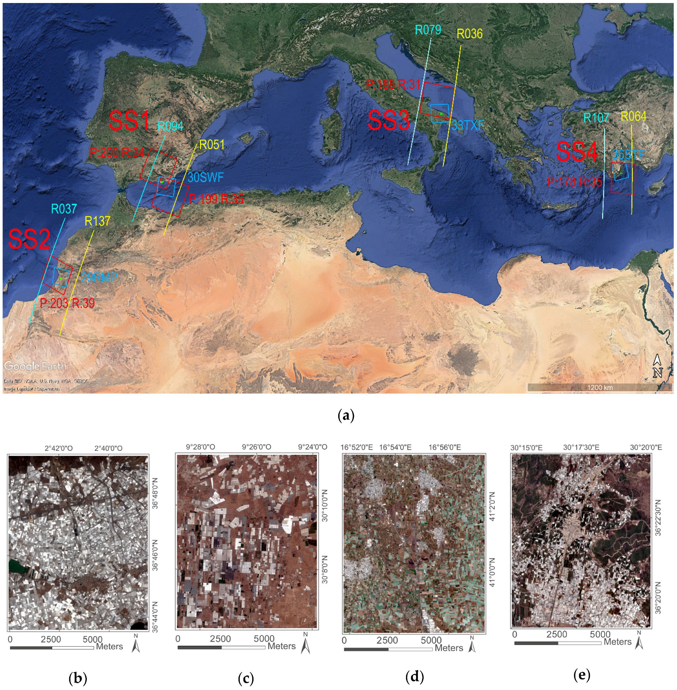
2. Study Sites
3. Datasets and Pre-Processing
4. Methods
4.1. Inter-Sensor Radiometric Coherence
4.2. Comparison Metrics
5. Results
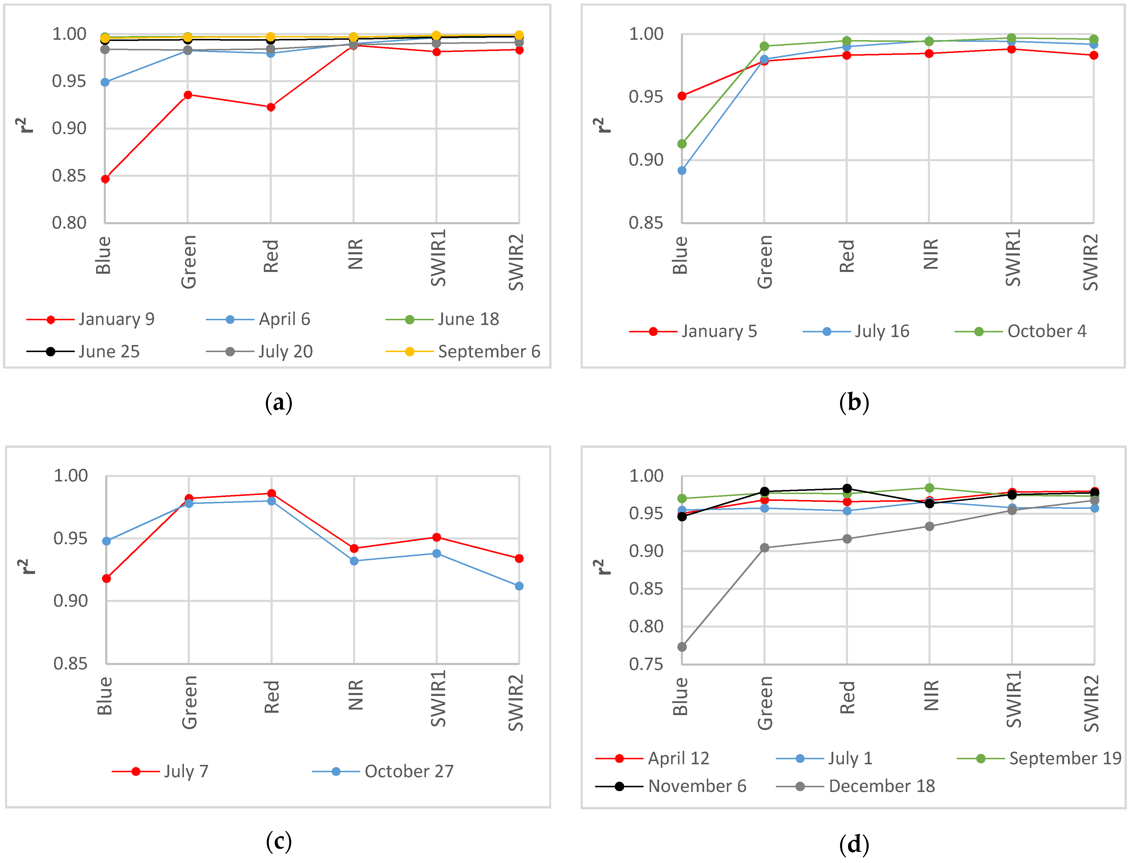
5.1. Inter-Sensor Radiometric Coherence between L8 Products
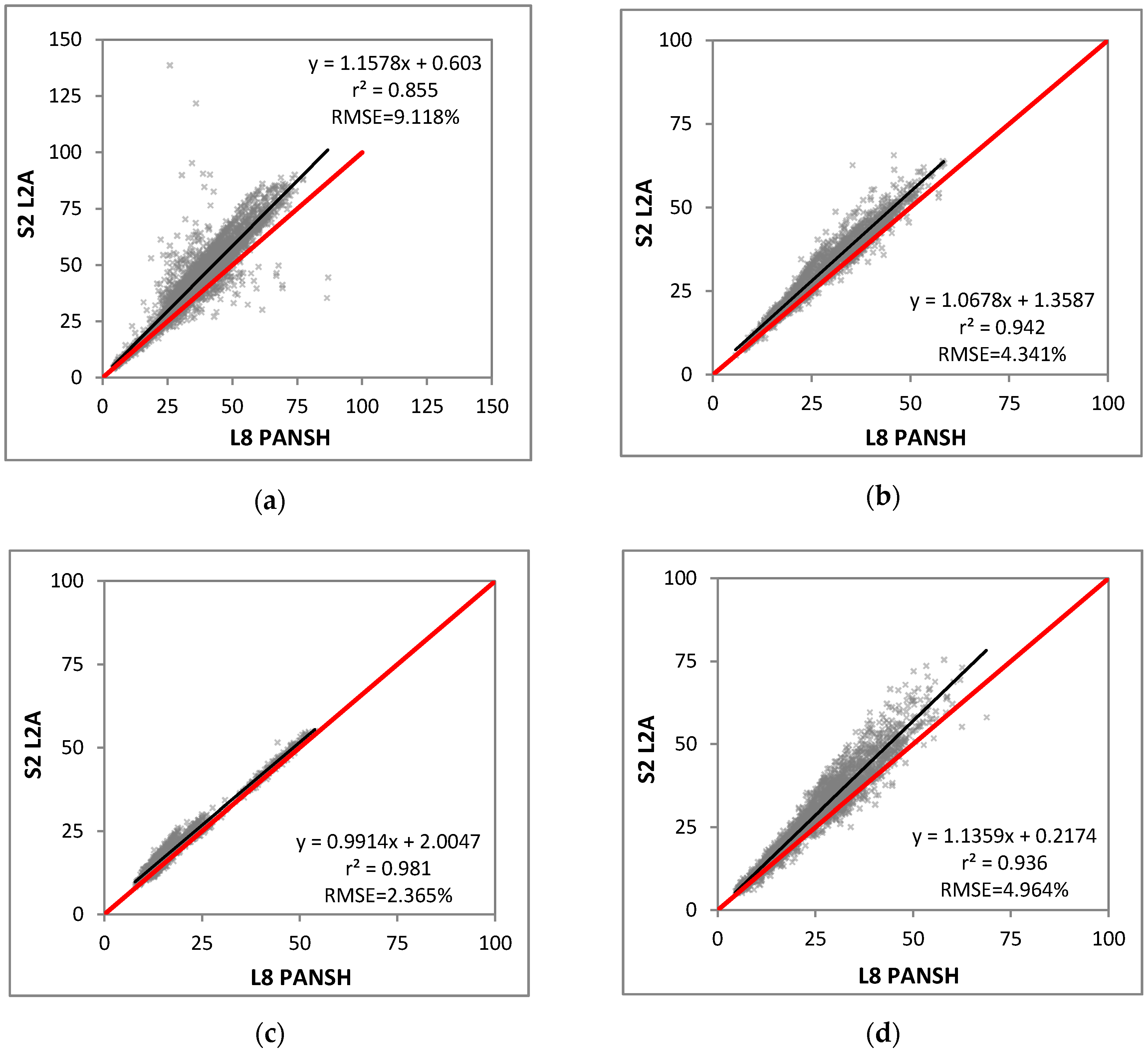
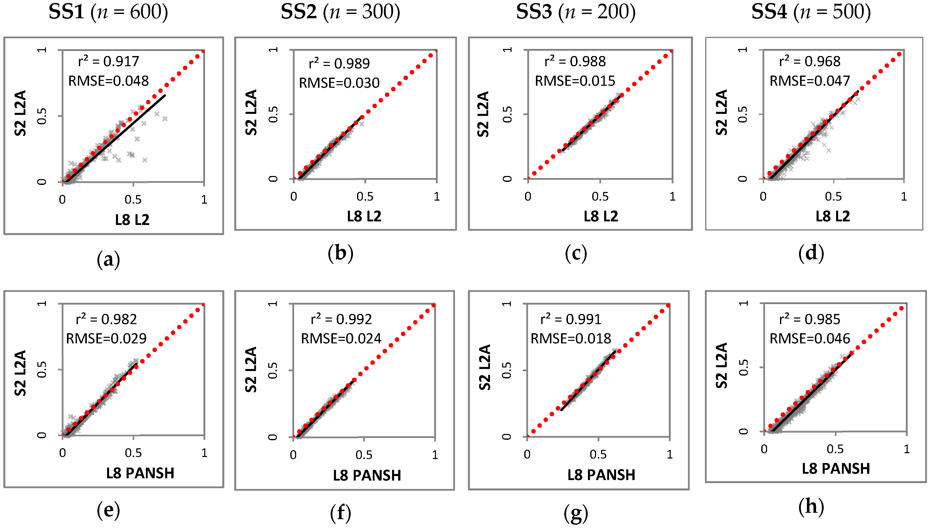
5.2. Consistency between L8 and S2 Products
5.3. NDVI Comparison
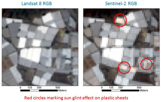
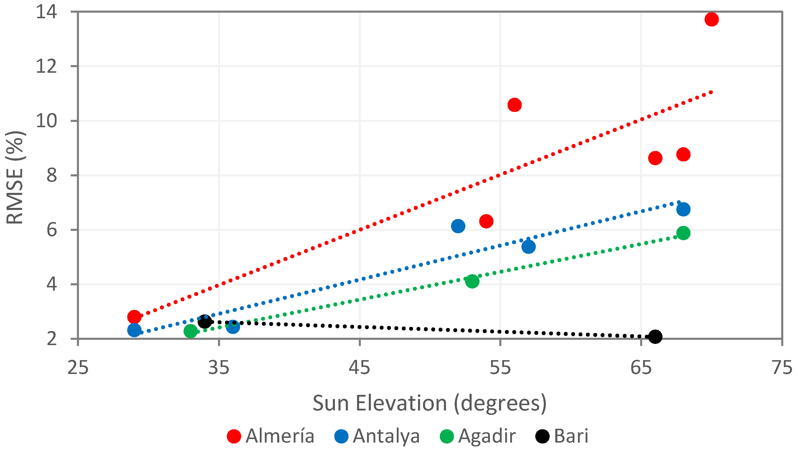
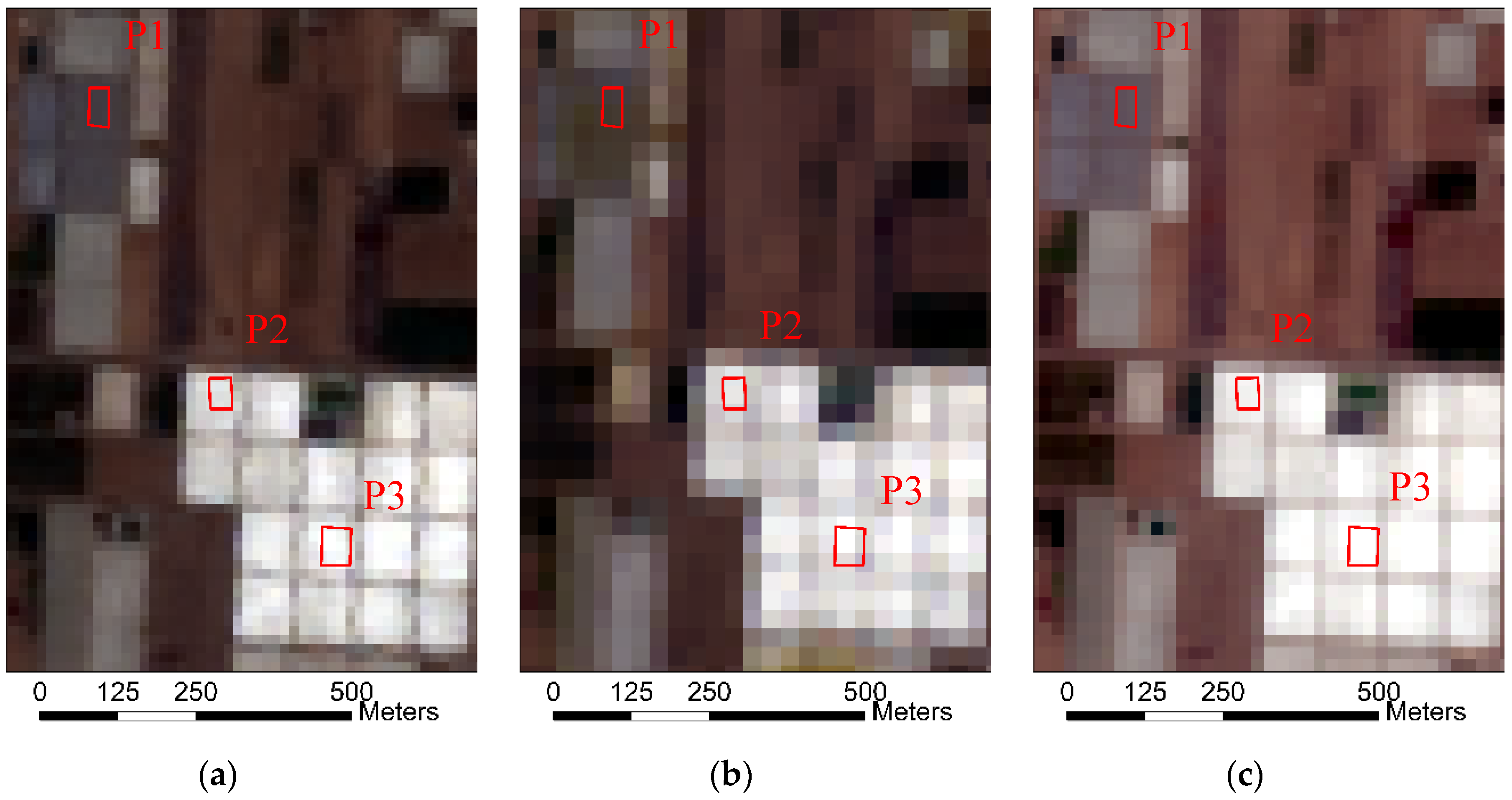
5.4. Sunglint Effects on PCG Areas
6. Discussion
7. Conclusions
Author Contributions
Funding
Acknowledgments
Conflicts of Interest
References
- Foley, J.A.; Ramankutty, N.; Brauman, K.A.; Cassidy, E.S.; Gerber, J.S.; Johnston, M.; Mueller, N.D.; O’Connell, C.; Ray, D.K.; West, P.C.; et al. Solutions for a Cultivated Planet. Nature 2011, 478, 337–342. [Google Scholar] [CrossRef] [PubMed] [Green Version]
- Jensen, M.H.; Malter, A.J. Protected Agriculture: A Global Review; World Bank Publications: Washington, DC, USA, 1995; Volume 253. [Google Scholar]
- Lamont, W.J.J. Overview of the use of high tunnels worldwide. HortTechnology 2009, 19, 25–29. [Google Scholar] [CrossRef] [Green Version]
- Espi, E.; Salmerón, A.; Fontecha, A.; García, Y.; Real, A.I. Plastic films for agricultural applications. J. Plast. Film Sheeting 2006, 22, 85–102. [Google Scholar] [CrossRef]
- Briassoulis, D.; Dougka, G.; Dimakogianni, D.; Vayas, I. Analysis of the collapse of a greenhouse with vaulted roof. Biosyst. Eng. 2016, 151, 495–509. [Google Scholar] [CrossRef]
- Agüera, F.; Aguilar, M.A.; Aguilar, F.J. Detecting greenhouse changes from QB imagery on the Mediterranean Coast. Int. J. Remote Sens. 2006, 27, 4751–4767. [Google Scholar] [CrossRef] [Green Version]
- Picuno, P.; Tortora, A.; Capobianco, R.L. Analysis of plasticulture landscapes in southern Italy through remote sensing and solid modelling techniques. Landsc. Urban Plan. 2011, 100, 45–56. [Google Scholar] [CrossRef]
- Jambeck, J.R.; Geyer, R.; Wilcox, C.; Siegler, T.R.; Perryman, M.; Andrady, A.; Narayan, R.; Law, K.L. Plastic waste inputs from land into the ocean. Mar. Pollut. 2015, 347, 768–771. [Google Scholar] [CrossRef]
- Lu, L.; Di, L.; Ye, Y. A Decision-Tree classifier for extracting transparent Plastic-Mulched landcover from landsat-5 TM images. IEEE J. Sel. Top. Appl. Earth Observ. Remote Sens. 2014, 7, 4548–4558. [Google Scholar] [CrossRef]
- Aguilar, M.A.; Vallario, A.; Aguilar, F.J.; García Lorca, A.; Parente, C. Object-Based Greenhouse Horticultural Crop Identification from Multi-Temporal Satellite Imagery: A Case Study in Almeria, Spain. Remote Sens. 2015, 7, 7378–7401. [Google Scholar] [CrossRef] [Green Version]
- Aguilar, M.A.; Nemmaoui, A.; Novelli, A.; Aguilar, F.J.; García Lorca, A. Object-Based Greenhouse Mapping Using Very High Resolution Satellite Data and Landsat 8 Time Series. Remote Sens. 2016, 8, 513. [Google Scholar] [CrossRef] [Green Version]
- Novelli, A.; Tarantino, E. Combining ad hoc spectral indices based on Landsat-8 OLI/TIRS sensor data for the detection of plastic cover vineyard. Remote Sens. Lett. 2015, 6, 933–941. [Google Scholar] [CrossRef]
- Wu, C.F.; Deng, J.S.; Wang, K.; Ma, L.G.; Tahmassebi, A.R.S. Object-based classification approach for greenhouse mapping using Landsat-8 imagery. Int. J. Agric. Biol. Eng. 2016, 9, 79–88. [Google Scholar] [CrossRef]
- Hasituya; Chen, Z. Mapping Plastic-Mulched Farmland with Multi-Temporal Landsat-8 Data. Remote Sens. 2017, 9, 557. [Google Scholar] [CrossRef] [Green Version]
- Yang, D.; Chen, J.; Zhou, Y.; Chen, X.; Chen, X.; Cao, X. Mapping plastic greenhouse with medium spatial resolution satellite data: Development of a new spectral index. ISPRS J. Photogramm. Remote Sens. 2017, 128, 47–60. [Google Scholar] [CrossRef]
- González-Yebra, Ó.; Aguilar, M.A.; Nemmaoui, A.; Aguilar, F.J. Methodological proposal to assess plastic greenhouses land cover change from the combination of archival aerial orthoimages and Landsat data. Biosyst. Eng. 2018, 175, 36–51. [Google Scholar] [CrossRef]
- Ou, C.; Yang, J.; Du, Z.; Liu, Y.; Feng, Q.; Zhu, D. Long-Term Mapping of a Greenhouse in a Typical Protected Agricultural Region Using Landsat Imagery and the Google Earth Engine. Remote Sens. 2020, 12, 55. [Google Scholar] [CrossRef] [Green Version]
- Levin, N.; Lugassi, R.; Ramon, U.; Braun, O.; Ben-Dor, E. Remote sensing as a tool for monitoring plasticulture in agricultural landscapes. Int. J. Remote Sens. 2007, 28, 183–202. [Google Scholar] [CrossRef]
- Hasituya; Chen, Z.; Wang, L.; Liu, J. Selecting Appropriate Spatial Scale for Mapping Plastic-Mulched Farmland with Satellite Remote Sensing Imagery. Remote Sens. 2017, 9, 265. [Google Scholar] [CrossRef] [Green Version]
- Drusch, M.; Del Bello, U.; Carlier, S.; Colin, O.; Fernandez, V.; Gascon, F.; Hoersch, B.; Isola, C.; Laberinti, P.; Martimort, P.; et al. Sentinel-2: ESA’s Optical High-Resolution Mission for GMES Operational Services. Remote Sens. Environ. 2012, 120, 25–36. [Google Scholar] [CrossRef]
- Lu, L.; Tao, Y.; Di, L. Object-Based Plastic-Mulched Landcover Extraction Using Integrated Sentinel-1 and Sentinel-2 Data. Remote Sens. 2018, 10, 1820. [Google Scholar] [CrossRef] [Green Version]
- Balcik, F.B.; Senel, G.; Goksel, C. Greenhouse Mapping using Object Based Classification and Sentinel-2 Satellite Imagery. In Proceedings of the 8th International Conference on Agro-Geoinformatics, Istanbul, Turkey, 16–19 July 2019; pp. 1–5. [Google Scholar] [CrossRef]
- Hao, P.; Chen, Z.; Tang, H.; Li, D.; Li, H. New Workflow of Plastic-Mulched Farmland Mapping using Multi-Temporal Sentinel-2 data. Remote Sens. 2019, 11, 1353. [Google Scholar] [CrossRef] [Green Version]
- Perilla, G.A.; Mas, J.F. High-resolution mapping of protected agriculture in Mexico, through remote sensing data cloud geoprocessing. Eur. J. Remote Sens. 2019, 52, 532–541. [Google Scholar] [CrossRef] [Green Version]
- Novelli, A.; Aguilar, M.A.; Nemmaoui, A.; Aguilar, F.J.; Tarantino, E. Performance evaluation of object based greenhouse detection fromSentinel-2 MSI and Landsat 8 OLI data: A case study from Almería(Spain). Int. J. Appl. Earth Obs. Geoinf. 2016, 52, 403–411. [Google Scholar] [CrossRef] [Green Version]
- Nemmaoui, A.; Aguilar, M.A.; Aguilar, F.J.; Novelli, A.; García Lorca, A. Greenhouse crop identification from multi-temporal multi-sensor satellite imagery using object-based approach: A case study from Almería (Spain). Remote Sens. 2018, 10, 1751. [Google Scholar] [CrossRef] [Green Version]
- Xiong, Y.; Zhang, Q.; Chen, X.; Bao, A.; Zhang, J.; Wang, Y. Large Scale Agricultural Plastic Mulch Detecting and Monitoring with Multi-Source Remote Sensing Data: A Case Study in Xinjiang, China. Remote Sens. 2019, 11, 2088. [Google Scholar] [CrossRef] [Green Version]
- Main-Knorn, M.; Pflug, B.; Debaecker, V.; Louis, J. Calibration and validation plan for the L2A processor and products of the Sentinel-2 mission. Int. Arch. Photogramm. Remote Sens. Spat. Inf. Sci. 2015, XL-7/W3, 1249–1255. [Google Scholar] [CrossRef] [Green Version]
- United States Geological Survey (USGS). EarthExplorer Download Tool. Available online: https://earthexplorer.usgs.gov/ (accessed on 9 April 2020).
- Vermote, E.; Justice, C.; Claverie, M.; Franch, B. Preliminary analysis of the performance of the Landsat 8/OLI land surface reflectance product. Remote Sens. Environ. 2016, 185, 46–56. [Google Scholar] [CrossRef]
- European Space Agency (ESA). Copernicus Open Access Hub. Available online: https://scihub.copernicus.eu/dhus/#/home (accessed on 9 April 2020).
- Li, J.; Roy, D.P. A Global Analysis of Sentinel-2A, Sentinel-2B and Landsat-8 Data Revisit Intervals and Implications for Terrestrial Monitoring. Remote Sens. 2017, 9, 902. [Google Scholar] [CrossRef] [Green Version]
- Mandanici, E.; Bitelli, G. Preliminary comparison of Sentinel-2 and Landsat 8 imagery for a combined use. Remote Sens. 2016, 8, 1014. [Google Scholar] [CrossRef] [Green Version]
- Lessio, A.; Fissore, V.; Borgogno-Mondino, E. Preliminary tests and results concerning integration of sentinel-2 and Landsat-8 OLI for crop monitoring. J. Imaging 2017, 3, 49. [Google Scholar] [CrossRef] [Green Version]
- Padró, J.-C.; Pons, X.; Aragonés, D.; Díaz-Delgado, R.; García, D.; Bustamante, J.; Pesquer, L.; Domingo-Marimon, C.; González-Guerrero, O.; Cristóbal, J.; et al. Radiometric Correction of Simultaneously Acquired Landsat-7/Landsat-8 and Sentinel-2A Imagery Using Pseudoinvariant Areas (PIA): Contributing to the Landsat Time Series Legacy. Remote Sens. 2017, 9, 1319. [Google Scholar] [CrossRef] [Green Version]
- Zhang, H.K.; Roy, D.P.; Yan, L.; Li, Z.; Huang, H.; Vermote, E.; Skakun, S.; Roger, J.-C. Characterization of Sentinel-2A Landsat-8 Top of Atmosphere, Surface, and Nadir BRDF Adjusted, Reflectance and NDVI Differences. Remote Sens. Environ. 2018, 215, 482–494. [Google Scholar] [CrossRef]
- Chastain, R.; Housman, I.; Goldstein, J.; Finco, M. Empirical cross sensor comparison of Sentinel-2A and 2B MSI, Landsat-8 OLI, and Landsat-7 ETM+ top of atmosphere spectral characteristics over the conterminous United States. Remote Sens. Environ. 2019, 221, 274–285. [Google Scholar] [CrossRef]
- Nie, Z.; Chan, K.K.Y.; Xu, B. Preliminary Evaluation of the Consistency of Landsat 8 and Sentinel-2 Time Series Products in An Urban Area—An Example in Beijing, China. Remote Sens. 2019, 11, 2957. [Google Scholar] [CrossRef] [Green Version]
- Arekhi, M.; Goksel, C.; Balik Sanli, F.; Senel, G. Comparative Evaluation of the Spectral and Spatial Consistency of Sentinel-2 and Landsat-8 OLI Data for Igneada Longos Forest. ISPRS Int. J. Geo-Inf. 2019, 8, 56. [Google Scholar] [CrossRef] [Green Version]
- Doxani, G.; Vermote, E.; Roger, J.-C.; Gascon, F.; Adriaensen, S.; Frantz, D.; Hagolle, O.; Hollstein, A.; Kirches, G.; Li, F.; et al. Atmospheric Correction Inter-Comparison Exercise. Remote Sens. 2018, 10, 352. [Google Scholar] [CrossRef] [Green Version]
- Claverie, M.; Ju, J.; Masek, J.G.; Dungan, J.L.; Vermote, E.F.; Roger, J.-C.; Skakun, S.V.; Justice, C.O. The Harmonized Landsat and Sentinel-2 surface reflectance data set. Remote Sens. Environ. 2018, 219, 145–161. [Google Scholar] [CrossRef]
- U.S. Geological Survey. Landsat 8 Surface Reflectance Code (LaSRC) Product Guide, Version 2.0. Department of the Interior, U.S. Geological Survey, 2019. Available online: https://www.usgs.gov/media/files/land-surface-reflectance-code-lasrc-product-guide (accessed on 23 April 2020).
- Defourny, P.; Bontemps, S.; Bellemans, N.; Cara, C.; Dedieu, G.; Guzzonato, E.; Hagolle, O.; Inglada, J.; Nicola, L.; Rabaute, T.; et al. Near real-time agriculture monitoring at national scale at parcel resolution: Performance assessment of the Sen2-Agri automated system in various cropping systems around the world. Remote Sens. Environ. 2019, 221, 551–568. [Google Scholar] [CrossRef]
- Berk, A.; Bernstein, L.S.; Anderson, G.P.; Acharya, P.K.; Robertson, D.C.; Chetwynd, J.H.; Adler-Golden, S.M. MODTRAN Cloud and Multiple Scattering Upgrades with Application to AVIRIS. Remote Sens. Environ. 1998, 65, 367–375. [Google Scholar] [CrossRef]
- Stumpf, A.; Michéa, D.; Malet, J.-P. Improved Co-Registration of Sentinel-2 and Landsat-8 Imagery for Earth Surface Motion Measurements. Remote Sens. 2018, 10, 160. [Google Scholar] [CrossRef] [Green Version]
- Li, Y.; Chen, J.; Ma, Q.; Zhang, H.K.; Liu, J. Evaluation of Sentinel-2A surface reflectance derived using Sen2Cor in North America. IEEE J. Sel. Top. Appl. Earth Obs. Remote. Sens. 2018, 11, 1997–2021. [Google Scholar] [CrossRef]
- Rouse, J.W.; Haas, R.H.; Schell, J.A.; Deering, D.W. Monitoring Vegetation Systems in the Great Plains with ERTS. In Proceedings of the 1973 Earth Resources Technology Satellite-1 Symposium, Washington, DC, USA, 10–14 December 1973. [Google Scholar]
- Aguilar, M.A.; Bianconi, F.; Aguilar, F.J.; Fernández, I. Object-based greenhouse classification from GeoEye-1 and WorldView-2 stereo imagery. Remote Sens. 2014, 6, 3554–3582. [Google Scholar] [CrossRef] [Green Version]
- Kokhanovsky, A.A. Aerosol Optics: Light Absorption and Scattering by Particles in the Atmosphere; Praxis Publishing Ltd.: Chichester, UK, 2008. [Google Scholar]
- Liang, S. Quantitative Remote Sensing of Land Surfaces; Wiley: Hoboken, NJ, USA, 2004. [Google Scholar]
- Shang, R.; Zhu, Z. Harmonizing Landsat 8 and Sentinel-2: A time-series-based reflectance adjustment approach. Remote Sens. Environ. 2019, 235, 111439. [Google Scholar] [CrossRef]
- Vuolo, F.; Zółtak, M.; Pipitone, C.; Zappa, L.; Wenng, H.; Immitzer, M.; Weiss, M.; Baret, F.; Atzberger, C. Data Service Platform for Sentinel-2 Surface Reflectance and Value-Added Products: System Use and Examples. Remote Sens. 2016, 8, 938. [Google Scholar] [CrossRef] [Green Version]
- Kay, S.; Hedley, J.; Lavender, S. Sun Glint Correction of High and Low Spatial Resolution Images of Aquatic Scenes: A Review of Methods for Visible and Near-Infrared Wavelengths. Remote Sens. 2009, 1, 697–730. [Google Scholar] [CrossRef] [Green Version]
- Pahlevan, N.; Schott, J.R.; Franz, B.A.; Zibordi, G.; Markham, B.; Bailey, S.; Schaaf, C.B.; Ondrusek, M.; Greb, S.; Strait, C.M. Landsat 8 remote sensing reflectance (Rrs) products: Evaluations, intercomparisons, and enhancements. Remote Sens. Environ. 2017, 190, 289–301. [Google Scholar] [CrossRef]
- Pahlevan, N.; Sarkar, S.; Franz, B.A.; Balasubramanian, S.V.; He, J. Sentinel-2 MultiSpectral Instrument (MSI) data processing for aquatic science applications: Demonstrations and validations. Remote Sens. Environ. 2017, 201, 47–56. [Google Scholar] [CrossRef]
- Aguilar, M.A.; Nemmaoui, A.; Aguilar, F.J.; Qin, R. Quality assessment of digital surface models extracted from WorldView-2 and WorldView-3 stereo pairs over different land covers. GISci. Remote Sens. 2019, 56, 109–129. [Google Scholar] [CrossRef] [Green Version]
- Scheffler, D.; Frantz, D.; Segl, K. Spectral harmonization and red edge prediction of Landsat-8 to Sentinel-2 using land cover optimized multivariate regressors. Remote Sens. Environ. 2020, 241, 111723. [Google Scholar] [CrossRef]
- Scheffler, D. SpecHomo: A Python Package for Spectral Homogenization of Multispectral Satellite Data (Version v 0.6.0). Zenodo. Available online: https://zenodo.org/record/3678744#.XvBAQOdRVPY (accessed on 23 April 2020). [CrossRef]


| Study Site | Date of Acquisition (D/M/Y) | Satellite | Path/Orbit | Row/ID Tile | Start Time (UTC) | Sun Azimuth (Degrees) | Sun Elevation (Degrees) |
|---|---|---|---|---|---|---|---|
| SS1: Almería (Spain) | 9 January 2019 | L8 (L1T-L2) | 199 | 35 | 10:44:16 | 156.13 | 28.02 |
| S2A (L2A) | R094 | 30SWF | 10:56:16 | 162.54 | 29.33 | ||
| 6 April 2019 | L8 (L1T-L2) | 200 | 34 | 10:49:42 | 142.66 | 53.38 | |
| S2A (L2A) | R051 | 30SWF | 10:01:06 | 147.41 | 55.80 | ||
| 18 June 2019 | L8 (L1T-L2) | 199 | 35 | 10:44:15 | 118.75 | 67.73 | |
| S2A (L2A) | R094 | 30SWF | 11:11:04 | 131.58 | 71.63 | ||
| 25 June 2019 | L8 (L1T-L2) | 200 | 34 | 10:50:04 | 121.67 | 66.97 | |
| S2A (L2A) | R051 | 30SWF | 11:01:09 | 125.79 | 69.82 | ||
| 20 July 2019 | L8 (L1T-L2) | 199 | 35 | 10:44:22 | 121.96 | 65.05 | |
| S2B (L2A) | R051 | 30SWF | 11:01:13 | 129.21 | 67.26 | ||
| 6 September 2019 | L8 (L1T-L2) | 199 | 35 | 10:44:37 | 144.76 | 54.98 | |
| S2A (L2A) | R094 | 30SWF | 11:11:00 | 153.17 | 57.21 | ||
| SS2: Agadir (Morocco) | 5 January 2019 | L8 (L1T-L2) | 203 | 39 | 11:10:35 | 154.20 | 32.49 |
| S2A (L2A) | R037 | 29RMP | 11:32:51 | 160.24 | 34.52 | ||
| 16 July 2019 | L8 (L1T-L2) | 203 | 39 | 11:10:40 | 107.29 | 67.01 | |
| S2B (L2A) | R137 | 29RMP | 11:23:10 | 111.31 | 69.81 | ||
| 4 October 2019 | L8 (L1T-L2) | 203 | 39 | 11:11:05 | 148.74 | 50.80 | |
| S2B (L2A) | R137 | 29RMP | 11:23:02 | 153.49 | 55.22 | ||
| SS3: Bari (Italy) | 7 July 2019 | L8 (L1T-L2) | 188 | 31 | 09:34:45 | 131.36 | 64.13 |
| S2A (L2A) | R079 | 33TXF | 09:59:19 | 142.03 | 67.86 | ||
| 27 October 2019 | L8 (L1T-L2) | 188 | 31 | 09:35:14 | 161.85 | 33.68 | |
| S2B (L2A) | R036 | 33TXF | 09:49:19 | 165.89 | 35.12 | ||
| SS4: Antalya (Turkey) | 12 April 2019 | L8 (L1T-L2) | 178 | 35 | 08:34:06 | 139.54 | 56.42 |
| S2B (L2A) | R064 | 36STF | 08:50:16 | 146.15 | 57.94 | ||
| 1 July 2019 | L8 (L1T-L2) | 178 | 35 | 08:34:32 | 118.33 | 67.08 | |
| S2B (L2A) | R064 | 36STF | 08:50:19 | 125.61 | 69.41 | ||
| 19 September 2019 | L8 (L1T-L2) | 178 | 35 | 08:34:55 | 148.22 | 51.14 | |
| S2B (L2A) | R064 | 36STF | 08:50:10 | 153.90 | 52.13 | ||
| 6 November 2019 | L8 (L1T-L2) | 178 | 35 | 08:35:00 | 160.09 | 35.68 | |
| S2A (L2A) | R107 | 36STF | 09:00:09 | 167.28 | 36.59 | ||
| 8 December 2019 | L8 (L1T-L2) | 178 | 35 | 08:34:56 | 160.26 | 28.64 | |
| S2B (L2A) | R064 | 36STF | 08:50:05 | 163.99 | 29.08 |
| Acquisition Dates (Aerosol) | Measures | Blue | Green | Red | NIR | SWIR1 | SWIR2 | All Bands |
|---|---|---|---|---|---|---|---|---|
| 9/1/2019 (13.2%) | RMSE | 4.110 | 3.581 | 3.719 | 2.559 | 2.193 | 2.028 | 3.136 |
| r2 | 0.808 | 0.880 | 0.868 | 0.886 | 0.921 | 0.921 | 0.941 | |
| 6/4/2019 (9.5%) | RMSE | 12.058 | 8.496 | 6.743 | 5.426 | 2.444 | 2.238 | 7.112 |
| r2 | 0.941 | 0.976 | 0.973 | 0.969 | 0.990 | 0.994 | 0.932 | |
| 18/6/2019 (1.4%) | RMSE | 12.205 | 11.325 | 11.625 | 12.593 | 16.592 | 19.513 | 14.300 |
| r2 | 0.815 | 0.738 | 0.571 | 0.308 | 0.069 | 0.038 | 0.340 | |
| 25/6/2019 (0.9%) | RMSE | 13.394 | 10.813 | 8.943 | 6.701 | 7.405 | 8.051 | 9.494 |
| r2 | 0.907 | 0.886 | 0.837 | 0.725 | 0.467 | 0.374 | 0.600 | |
| 20/7/2019 (0.1%) | RMSE | 14.271 | 12.057 | 10.050 | 6.611 | 5.141 | 7.463 | 9.797 |
| r2 | 0.988 | 0.988 | 0.988 | 0.991 | 0.993 | 0.994 | 0.897 | |
| 6/9/2019 (1.2%) | RMSE | 18.198 | 15.087 | 12.171 | 8.192 | 5.122 | 5.838 | 11.792 |
| r2 | 0.972 | 0.973 | 0.972 | 0.960 | 0.954 | 0.954 | 0.865 |
| Acquisition Dates (Aerosol) | Measures | Blue | Green | Red | NIR | SWIR1 | SWIR2 | All Bands |
|---|---|---|---|---|---|---|---|---|
| 5/1/2019 (5.2%) | RMSE | 3.797 | 3.373 | 2.868 | 2.445 | 1.898 | 1.914 | 2.807 |
| r2 | 0.940 | 0.970 | 0.973 | 0.971 | 0.987 | 0.986 | 0.976 | |
| 16/7/2019 (33.0%) | RMSE | 9.706 | 7.132 | 6.116 | 4.151 | 4.946 | 7.410 | 6.820 |
| r2 | 0.840 | 0.919 | 0.921 | 0.904 | 0.833 | 0.727 | 0.850 | |
| 4/10/2019 (14.1%) | RMSE | 6.526 | 4.970 | 4.221 | 2.931 | 3.217 | 5.180 | 4.671 |
| r2 | 0.901 | 0.987 | 0.992 | 0.989 | 0.993 | 0.994 | 0.946 |
| Acquisition Dates (Aerosol) | Measures | Blue | Green | Red | NIR | SWIR1 | SWIR2 | All Bands |
|---|---|---|---|---|---|---|---|---|
| 7/7/2019 (6.7%) | RMSE | 3.971 | 2.769 | 1.279 | 2.338 | 1.081 | 1.039 | 2.338 |
| r2 | 0.914 | 0.972 | 0.981 | 0.905 | 0.930 | 0.904 | 0.904 | |
| 27/10/2019 (3.1%) | RMSE | 4.228 | 3.079 | 1.803 | 2.492 | 2.336 | 2.256 | 2.809 |
| r2 | 0.938 | 0.969 | 0.976 | 0.923 | 0.950 | 0.937 | 0.985 |
| Acquisition Dates (Aerosol) | Measures | Blue | Green | Red | NIR | SWIR1 | SWIR2 | All Bands |
|---|---|---|---|---|---|---|---|---|
| 12/4/2019 (20.3%) | RMSE | 9.623 | 7.098 | 5.665 | 4.183 | 2.615 | 2.537 | 5.857 |
| r2 | 0.930 | 0.951 | 0.947 | 0.931 | 0.945 | 0.951 | 0.907 | |
| 1/7/2019 (5.0%) | RMSE | 11.348 | 8.830 | 7.279 | 4.179 | 3.905 | 4.941 | 7.267 |
| r2 | 0.928 | 0.933 | 0.942 | 0.951 | 0.940 | 0.899 | 0.872 | |
| 19/9/2019 (5.7%) | RMSE | 9.785 | 8.056 | 6.858 | 3.422 | 3.426 | 4.642 | 6.489 |
| r2 | 0.938 | 0.961 | 0.968 | 0.971 | 0.975 | 0.984 | 0.889 | |
| 6/11/2019 (9.5%) | RMSE | 3.132 | 2.611 | 2.190 | 2.063 | 1.321 | 1.302 | 2.203 |
| r2 | 0.913 | 0.941 | 0.951 | 0.772 | 0.915 | 0.948 | 0.957 | |
| 18/12/2019 (29.9%) | RMSE | 3.269 | 2.195 | 1.984 | 2.385 | 1.833 | 1.729 | 2.291 |
| r2 | 0.703 | 0.830 | 0.868 | 0.642 | 0.899 | 0.964 | 0.951 |
© 2020 by the authors. Licensee MDPI, Basel, Switzerland. This article is an open access article distributed under the terms and conditions of the Creative Commons Attribution (CC BY) license (http://creativecommons.org/licenses/by/4.0/).
Share and Cite
Aguilar, M.Á.; Jiménez-Lao, R.; Nemmaoui, A.; Aguilar, F.J.; Koc-San, D.; Tarantino, E.; Chourak, M. Evaluation of the Consistency of Simultaneously Acquired Sentinel-2 and Landsat 8 Imagery on Plastic Covered Greenhouses. Remote Sens. 2020, 12, 2015. https://doi.org/10.3390/rs12122015
Aguilar MÁ, Jiménez-Lao R, Nemmaoui A, Aguilar FJ, Koc-San D, Tarantino E, Chourak M. Evaluation of the Consistency of Simultaneously Acquired Sentinel-2 and Landsat 8 Imagery on Plastic Covered Greenhouses. Remote Sensing. 2020; 12(12):2015. https://doi.org/10.3390/rs12122015
Chicago/Turabian StyleAguilar, Manuel Ángel, Rafael Jiménez-Lao, Abderrahim Nemmaoui, Fernando José Aguilar, Dilek Koc-San, Eufemia Tarantino, and Mimoun Chourak. 2020. "Evaluation of the Consistency of Simultaneously Acquired Sentinel-2 and Landsat 8 Imagery on Plastic Covered Greenhouses" Remote Sensing 12, no. 12: 2015. https://doi.org/10.3390/rs12122015
APA StyleAguilar, M. Á., Jiménez-Lao, R., Nemmaoui, A., Aguilar, F. J., Koc-San, D., Tarantino, E., & Chourak, M. (2020). Evaluation of the Consistency of Simultaneously Acquired Sentinel-2 and Landsat 8 Imagery on Plastic Covered Greenhouses. Remote Sensing, 12(12), 2015. https://doi.org/10.3390/rs12122015