An Estimation of Top-Down NO_x Emissions from OMI Sensor Over East Asia

Abstract

This study focuses on the estimation of top-down NO_x emissions over East Asia, integrating information on the levels of NO₂ and NO, wind vector, and geolocation from Ozone Monitoring Instrument (OMI) observations and Weather Research and Forecasting (WRF)-Community Multiscale Air Quality (CMAQ) model simulations. An algorithm was developed based on mass conservation to estimate the 30 km × 30 km resolved top-down NO_x emissions over East Asia. In particular, the algorithm developed in this study considered two main atmospheric factors—(i) NO_x transport from/to adjacent cells and (ii) calculations of the lifetimes of column NO_x (τ). In the sensitivity test, the analysis showed the improvements in the top-down NO_x estimation via filtering the data (τ ≤ 2 h). The best top-down NO_x emissions were inferred after the sixth iterations. Those emissions were 11.76 Tg N yr⁻¹ over China, 0.13 Tg N yr⁻¹ over North Korea, 0.46 Tg N yr⁻¹ over South Korea, and 0.68 Tg N yr⁻¹ over Japan. These values are 34%, 62%, 60%, and 47% larger than the current bottom-up NO_x emissions over these countries, respectively. A comparison between the CMAQ-estimated and OMI-retrieved NO₂ columns was made to confirm the accuracy of the newly estimated NO_x emission. The comparison confirmed that the estimated top-down NO_x emissions showed better agreements with observations (R² = 0.88 for January and 0.81 for July).

1. Introduction

Smog events in East Asia have been recognized as severe air pollution problems, resulting in deteriorated air quality in the atmosphere [1,2,3] and harmful effects on human health and the ecological system [4,5,6]. With growing public concerns, air quality forecasts have become an important issue. In this context, forecasting the short-term particulate matters of 10 and 2.5 (PM₁₀ and PM_2.5) and ozone concentrations has been nationally implemented in South Korea since February 2014. However, there has been a lack of capability in more accurately forecasting the levels of pollutants due to many uncertainties related to the meteorological fields, anthropogenic and biogenic emissions, chemical and physical parameterizations, boundary, and initial conditions, and land uses and land covers [7,8,9]. Among these uncertainties, the accuracy of emissions is one of the most important for improving the performance of air quality forecasting.

Air quality forecast (and general air quality modeling) heavily depends on the accuracy of emissions. It has also been well understood that among the pollutants, nitrogen oxides (NO_x = NO + NO₂) are important precursors for producing ozone and secondary inorganic aerosols. Despite such importance, the NO_x emissions in East Asia have still been highly uncertain [10,11,12,13,14].

Apart from constructing accurate bottom-up NO_x emission inventories, many studies have explored top-down NO_x estimations over megacities [15,16,17,18,19], several regions of Asia [20,21,22,23,24,25,26], Europe [27,28,29], North America [30,31,32,33,34], and on a global scale [35,36,37,38,39,40,41,42].

Many investigators have used an advanced inversion method of 4D-variation data assimilation [42,43,44,45] and Kalman Filter [39,41,46,47] to estimate the top-down NO_x emissions. However, the method is still computationally expensive despite better scalability on the hardware platform of parallel computing. On the other hand, the computational cost base on the mass balance approach is relatively low. Besides, in the comparison study, Cooper et al. showed that the mass balance approach for the NO_x estimations produces similar results to those from the adjoint method [42].

Table 1. Several estimations for top-down NO_x emissions based on the mass balance approach.

References	Methodology	Target Region and Year	NOx Emission
Leue et al. [48]	$\frac{d{\mathsf{\Omega }}_s}{dt}=\mathrm{E}-\frac{{\mathsf{\Omega }}_s}{\mathsf{\tau }}$ - E: emission strength (top-down NOx); $\mathrm{E}\approx \frac{{\mathsf{\Omega }}_s}{\mathsf{\tau }}$ - Ωs: satellite-derived NOx columns; - τ: NOx lifetime (constant value of 27 ± 3 h)	Global/ 1997	43.5 Tg N yr−1 (for the globe) 2.7 Tg N yr−1 (for China) 0.5 Tg N yr−1 (for Japan)
Martin et al. [35,36]	(i) Top-down NOx (Et): ${\mathrm{E}}_{\mathrm{t}}={\mathrm{E}}_{\mathrm{b}}\times \frac{{\mathsf{\Omega }}_s}{{\mathsf{\Omega }}_m}$ - Et: top-down NOx; - Eb: bottom-up (a priori) NOx; - Ωs: satellite-derived NO2 columns; - Ωm: CTM-derived NO2 column;	Global/ Sep. 1996– Aug. 1997	38.0 Tg N yr−1 (for the globe) 5.4 Tg N yr−1 (for East Asia)
	(ii) A posterior NOx (E, optimized NOx emissions) $\ln \mathrm{E}=\frac{\left(\ln {\mathrm{E}}_{\mathrm{t}}\right){\left(\ln {\epsilon }_b\right)}^2+\left(\ln {\mathrm{E}}_{\mathrm{b}}\right){\left(\ln {\epsilon }_t\right)}^2}{{\left(\ln {\epsilon }_b\right)}^2+{\left(\ln {\epsilon }_t\right)}^2}$ - εb: relative geometric error between a priori and EDGAR NOx emissions; - εt: relative geometric error between top-down and EDGAR NOx emissions	Global/Sep. 1996 − Aug. 1997	37.7 Tg N yr−1 (for the globe) 5.3 Tg N yr−1 (for East Asia)
Boersma et al. [30]	Basic concept from Martin et al. [35] ${\mathrm{E}}_{\mathrm{t}}=\frac{{\mathrm{E}}_{\mathrm{b}}}{{\displaystyle \sum {\displaystyle \sum \mathrm{K}{\mathrm{E}}_{\mathrm{b}}}}}{\mathrm{E}}_{\mathrm{b}}\times \frac{{\mathsf{\Omega }}_s}{{\mathsf{\Omega }}_m}$ Here, K (kernel) matrix defined as K - k: smoothing parameter $\mathrm{K}=\frac{1}{k+8}\left(\begin{array}{ccc}1& 1& 1\\ 1& k& 1\\ 1& 1& 1\end{array}\right)$ (k = 12 in the study)	Eastern US & Mexico/Mar. 2006	0.5 Tg N month−1 (for Eastern US) 0.1 Tg N month−1 (for Mexico)
Zhao and Wang [20]	Assimilated a posteriori based on Martin et al. [35]	East Asia/Jul. 2007	9.5 Tg N yr−1 (for East Asia)
Lamsal et al. [37,40]	Top-down NOx estimation from Martin et al. [35] and Boersma et al. [30]	N. America, Europe, and East Asia/2006–2007	7.6–8.9 Tg N yr−1 (for N. America) 3.9–5.2 Tg N yr−1 (for Europe) 10.9–13.1 Tg N yr−1 (for East Asia)
Lin et al. [21]	Concept based on study of Leue et al. [42], using multi-satellite data observed at different scanning time ${\mathrm{E}}_{\mathrm{t}}=\frac{{{\mathsf{\Omega }}_s|}_n-{{\mathsf{\Omega }}_s|}_0·e^{{\displaystyle \sum _{i=1}^{n-1}\left(-\Delta t/{\mathsf{\tau }}_i\right)}}}{{\displaystyle \sum _{i=0}^{n-1}\left({\mathrm{E}}_{\mathrm{i}}/\overline{\mathrm{E}}·\left(1-e^{-\Delta t/{\mathsf{\tau }}_i}\right)·{\mathsf{\tau }}_i\right)}}$ - Et: top-down NOx emission; - Ωs|n: satellite NOx columns at n-th hour; - Ωs|0: satellite NOx columns at 0-th hour; - τ: NOx lifetime; - Δt: time interval; - Ei: NOx emission at i-th hour; - Ē: daily mean of E	China/2008	6.8 Tg N yr−1 (best estimate for China)
Ghude et al. [22]	Basic concept from Martin et al. [35] ${\mathrm{E}}_{\mathrm{t}}={\mathrm{E}}_{\mathrm{b}}\times \frac{{\mathsf{\Omega }}_s}{{\mathsf{\Omega }}_m}$ - Ωm: model-predicted NO2 columns w/ consideration of averaging kernel	India/2005	1.9 Tg N yr−1 (for India)
Goldberg et al. [34]	$\mathrm{E}=1.33\frac{{\mathsf{\Omega }}_s}{\mathsf{\tau }}$ Exponentially modified Gaussian fitting method [15] - E: top-down NOx emission; $\mathsf{\tau }=x_0/\omega$ - Ωs: satellite-derived NO2 columns; - τ: effective NO2 lifetime; - 1.33: mean column-averaged NOx/NO2 ratio; - x0: e-fold distance downwind; - ω: mean zonal wind speed	South Korea/2016 (KORUS-AQ field campaign)	0.353 ± 0.146 Tg NOx yr-1 (for Seoul Metropolitan areas)

summarizes the various methodologies used for the estimations of NO_x emissions from the satellite observations, based on the mass conservation approach. Leue et al. first estimated the top-down NO_x emissions, using the Global Ozone Monitoring Experiment (GOME)-retrieved NO₂ data with the conversion factor of NO₂ to NO_x and a constant NO_x lifetime of 27 h [48]. However, the simple assumption in the NO_x lifetime possibly causes significant errors.

Martin et al. also estimated top-down NO_x emissions [35,36]. In their study, however, the transports of NO_x molecules from/to neighbor grid cells were neglected via the uses of very coarse horizontal resolution (2° × 2.5°) and relatively short NO_x lifetimes, particularly during the summer months. For the consideration of NO_x transport from/to the adjacent grid-cells, several investigators have introduced the smoothing kernels defined in Table 1 (e.g., references [30,37,40,49]). In Zhao and Wang [20], the issue of the NO_x transport was treated indirectly by assimilation using the OMI (Ozone Monitoring Instrument)-retrieved NO₂ columns on a daily basis. Another method was suggested by Lin et al. [21], who used multi-satellite NO₂ columns observed at different scanning times (e.g., GOME-2 for ~9:30 LT and OMI for ~13:45 LT). The methodology applied to a summer case, based on the hourly differences between two satellite-derived NO_x columns from the consistent retrieval algorithm and NO_x chemical evolution. However, as pointed out in their study, significant limitations can be met, when the suggested methodology applies to the high-resolved chemistry-transport model (3D-CTM) simulations or the winter case, resulting in a sufficiently long NO_x lifetime.

Many studies based on the mass balance approach have the relatively coarse-grid resolution (~1°) for the 3D-CTM simulations and focus on the estimations for summer episode. An alternative is required to estimate top-down NO_x emissions with a finer grid-resolution, particularly during the cold seasons. Therefore, the challenging goal of this study is to develop an algorithm for the top-down estimation of NO_x emissions with runs of 3D-CTM simulations in a 30 km × 30 km grid resolution and with the retrieval of OMI NO₂ columns. The manuscript was organized as followed. First, the research methods for the CTM simulations and satellite data are described in Section 2. The algorithm for the top-down estimations is fully described in Section 3. To evaluate and finally quantify NO_x emissions over East Asia, the CTM-simulated NO₂ columns are compared with the OMI-retrieved NO₂ columns in Section 4. Summary and conclusions are given in Section 5.

2. Experimental Methods

2.1. Description of WRF-CMAQ Model Simulations

The meteorological fields were generated by the Weather Research and Forecasting v3.4.1 (WRF) model [50] in conjunction with National Center for Environmental Prediction (NCEP) reanalysis data [51,52]. The WRF simulation was configured with the following atmospheric physical schemes: the Yonsei University (YSU) scheme for planetary boundary layer (PBL) physics [53], the five-layer thermal diffusion Land Surface Model (LSM) scheme for land surface, the Dudhia scheme for the shortwave radiation [54], the rapid radiative transfer model (RRTM) scheme for the longwave radiation [55]; and Kain–Fritsch scheme for the cumulus parametrization [56]. The output from the WRF simulations was then used to generate the model-ready meteorological input data via the meteorological chemistry interface process (MCIP) for the CMAQ model simulations.

The Community Multi-scale Air Quality (CMAQ) v4.7.1 model [57] was used over East Asia for January and July 2010. As shown in Figure 1, the CMAQ domain covered a region of East Asia (100°–145° E and 20°–50° N) including China, Korea, Japan, and some parts of Mongolia, Russia, and the northwest Pacific Ocean with a 30 × 30 km² horizontal resolution and 14 vertical levels from the surface to ~95 hPa. Lambert-conformal projection centered at 121° Longitude and 34° Latitude was applied. The main modules used in the CMAQ model simulations were the AERO4 for the aerosol dynamics and thermodynamics [58] and the Statewide Air Pollution Research Center-99 (SAPRC-99) mechanism for the gas-phase chemistry [59]. Other conditions for the CMAQ model simulations were described in the previous studies of Han et al. [14,60].

For emission inputs (i.e., a priori emission), the anthropogenic emissions from the Model Inter-comparison Study for Asia Phase III (MICS-Asia III) inventory compiled for the year 2010 were utilized for the CMAQ model simulations over East Asia. The MICS-Asia III emissions with 0.25° × 0.25° resolution were combined from several regional emission inventories such as MEIC v1.0 for China, CAPSS for South Korea, JEI-BD/OPRF for Japan, and REAS v2.1 for others, to best describe the emissions from the countries. Further information on the MICS-Asia III inventory was described in the studies of Li et al. and Janssens-Maenhout et al. [61,62]. For the consideration of biogenic emissions, the 0.5° × 0.5° resolved model of emission of gases and aerosols from nature-monitoring atmospheric composition and climate (MEGAN-MACC) emission inventory compiled for the same year of 2010 (http://eccad.sedoo.fr) were used [63]. Also, for fire emissions, the Quick Fire Emissions Dataset (QFED) v2.4 with 0.1° × 0.1° grid resolution was obtained from the NASA Center for Climate Simulation (NCCS) for the year of 2010 [64]. The fire emissions injected from the high altitudes can have a considerable impact on the transport of NO_x molecules in the model simulations [65,66]. However, we believe that such an effect is not significant in the monthly estimation of top-down NO_x emissions because these biomass burning NO_x emissions utilized in the current simulation account for ~0.01% of the total NO_x emissions in the entire domain. Soil NO_x emissions obtained from REAS v2.1 inventory [67] for the year of 2008 also accounted for 0.85 and 13.07% of the total NO_x emissions in January and July, respectively. In the CMAQ model simulations, other NO_x sources such as lightning and aircraft were not considered due to high uncertainties over East Asia [20].

2.2. Description of OMI NO₂ Columns

The OMI, one of four sensors on board the NASA/EOS-Aura satellite, has been used widely for the studies of atmospheric chemistry due to several advantages, particularly in the high spatial and temporal resolutions. The OMI instrument observes the atmosphere over East Asia at approximate 13:45 local time (LT) with a spatial resolution of 13 km × 24 km at the nadir.

The OMI-retrieved NO₂ columns, their errors, and averaging kernels (AKs) used in the study were described in detail by Boersma et al. [68,69]. Therefore, here, we briefly introduce some information on the daily OMI dataset retrieved from KNMI/DOMINO v2.0 algorithm. The tropospheric NO₂ columns from the OMI level-1b radiance data are retrieved in the following three steps. In the first step, NO₂ slant columns are obtained from the OMI reflectance spectra with a fitting window ranging between 405 nm and 465 nm, on the basis of the differential optical absorption spectroscopy (DOAS) technique [70]. In the second step, the stratospheric contributions to the total NO₂ slant columns are estimated to generate the tropospheric portions of the NO₂ slant columns. Here, the stratospheric NO₂ slant columns are calculated by assimilating OMI-measured NO₂ slant columns in a chemical data assimilation system [71]. In the last, the air mass factor (AMF) is introduced to convert the tropospheric NO₂ slant columns to the tropospheric NO₂ vertical columns. The errors of the individual tropospheric NO₂ columns in the DOMINO v2.0 are approximate 1.0 × 10¹⁵ molecules cm⁻², which are mostly due to the AMF calculations [69]. AMF is a function of surface albedo, terrain height, vertical profiles of clouds and aerosols, and the presence of trace gases. In this study, in order to reduce retrieval errors, only OMI data with cloud radiance fraction (CRFs) smaller than 50% and surface albedo smaller than 0.3 was used, as suggested by Boersma et al. [68].

For the top-down NO_x estimation in East Asia, we also took advantage of the “daily” levels of tropospheric OMI-retrieved NO₂ columns (level 2 product) obtained from the TEMIS (http://www.temis.nl). The conversion of NO₂ to NO_x columns was fully described in Section 3.5. The total errors in the tropospheric NO₂ columns applied to the estimations of NO_x emissions were 3.05 × 10¹⁵ and 7.47 × 10¹⁴ molecules cm⁻², which accounted for approximately 65% and 48% of the tropospheric NO₂ columns over the entire domain, in East Asia for January and July, respectively. Besides, several investigators identified significant low biases (e.g., 10% over Tokyo, 26–38% over Beijing) in the current OMI-retrieved tropospheric NO₂ columns, comparing with the Multi-Axis Differential Optical Absorption Spectroscopy (MAX-DOAS) observations over some regions in Canada, Greece, China, and Japan [72,73,74,75,76]. Accordingly, the top-down estimate in the study is likely underestimating the true one.

3. Algorithm for Top-Down Estimation of NO_x Emissions

The current study can be characterized by two main components: the considerations of (i) transport of NO_x molecules among the grid-cells and (ii) lifetimes of column NO_x. Two issues are explained in detail.

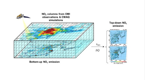
3.1. General Concept

The NO_x columns (Ω_NOx) in the troposphere can be determined by the balance among emission (E), chemical production (F), chemical/physical losses (L), and columnar NO_x transported from/to adjacent grid cells (Q_in and Q_out). The rate of change of Ω_NOx with respect to time can be expressed by the following Equation (1):

$$\frac{\partial {\mathsf{\Omega }}_{\mathrm{N}{\mathrm{O}}_{\mathrm{x}}}}{\partial t}=\mathrm{E}+\mathrm{F}-\mathrm{L}+{\mathrm{Q}}_{\mathrm{i}\mathrm{n}}-{\mathrm{Q}}_{\mathrm{o}\mathrm{u}\mathrm{t}}$$

(1)

The above equation can be converted into Equation (2):

$$\frac{\partial {\mathsf{\Omega }}_{\mathrm{N}{\mathrm{O}}_{\mathrm{x}}}}{\partial t}=\mathrm{E}-\frac{{\mathsf{\Omega }}_{\mathrm{N}{\mathrm{O}}_{\mathrm{x}}}}{\mathsf{\tau }}+\Delta \mathrm{Q}$$

(2)

where τ represents the lifetime of column NO_x, which includes the photo-chemical, physical, and meteorological removals or disappearance at a given grid cell. For the estimations of NO_x emissions (E), the data collected from the CMAQ model simulations were averaged between 13:00 and 14:00 LT for the ith time step, which is approximately consistent with the OMI scanning time over East Asia. The columnar NO_x at the ith time step (Ω_NOx,i) and emission (E) can be expressed via the following formulas (Equations (3)–(5)):

$${\mathsf{\Omega }}_{\mathrm{N}{\mathrm{O}}_{\mathrm{x},\mathrm{i}}}=\left(\mathrm{E}+\Delta \mathrm{Q}\right)·\mathsf{\tau }·\left(1-e^{-\Delta t/\mathsf{\tau }}\right)+{\mathsf{\Omega }}_{\mathrm{N}{\mathrm{O}}_{\mathrm{x},\mathrm{i}-1}}·e^{-\Delta t/\mathsf{\tau }}$$

(3)

$$f(\mathsf{\tau })=\left(\mathrm{E}+\Delta \mathrm{Q}\right)·\mathsf{\tau }·\left(e^{-1/\mathsf{\tau }}-1\right)-{\mathsf{\Omega }}_{\mathrm{N}{\mathrm{O}}_{\mathrm{x},\mathrm{i}-1}}·e^{-1/\mathsf{\tau }}+{\mathsf{\Omega }}_{\mathrm{N}{\mathrm{O}}_{\mathrm{x},\mathrm{i}}}=0$$

(4)

$$\mathrm{E}=\frac{{\mathsf{\Omega }}_{\mathrm{N}{\mathrm{O}}_{\mathrm{x},\mathrm{i}-1}}·e^{-\Delta t/\mathsf{\tau }}-{\mathsf{\Omega }}_{\mathrm{N}{\mathrm{O}}_{\mathrm{x},\mathrm{i}}}}{\mathsf{\tau }·\left(e^{-\Delta t/\mathsf{\tau }}-1\right)}-\Delta \mathrm{Q}$$

(5)

where Δt represents a time interval, which is corresponding to 1 h in this study. Other works can also be explained with Equation (5). For example, Lin et al. obtained Ω_NOx,i and Ω_NOx,i-1 from OMI and GOME-2 sensors, respectively, with Δt = 3 h and ΔQ = 0 in terms of Equation (5), to calculate top-down NO_x emissions [21].

The estimations of top-down NO_x proceeded as followed: First, the amounts of NO_x transported from/to adjacent cells (Q_in and Q_out) are calculated using the wind vectors and NO_x concentrations of each layer at the i-1th time step (refer to Figure 2 and Section 3.2 and Section 3.3). Second, the variables such as columnar NO_x at ith and i-1th time steps, bottom-up NO_x emission, and ΔQ are fed into the Equation (4) rearranged from Equation (3) to calculate τ. Third, we attempt to confirm whether the scientific approach chosen here is correct via re-calculating the bottom-up NO_x emissions using Equation (5). The re-calculated NO_x emissions should be equal to the bottom-up NO_x emissions used in the CMAQ model simulations. In the fourth step, for conducting a sensitivity analysis of τ, the top-down NO_x emission is estimated from Equation (5) using a columnar NO_x (Ω_NOx) based on the model results for the arbitrary satellite-observed data on the OMI footprint. In this step, the calculated top-down NO_x emissions from the arbitrary data should be the same as the (bottom-up) model input emissions. The arbitrary data can be used for sensitivity tests of the here presented method. The statistical analysis between the two sets of data was carried out with respect to τ to find the optimal condition for the top-down NO_x emissions in the final step. Finally, daily OMI-observed data are applied to the estimations of top-down NO_x emission over East Asia. The procedure was repeated until the differences between CMAQ-calculated and OMI-retrieved NO₂ columns are within the error tolerance. Further details can be found in the next sections.

3.2. NO_x Transported from Adjacent Cells (Q_in)

In many top-down NO_x estimations, the influx and outflux into/out of grid cells have been neglected, because of the use of sufficiently large grid resolution in the global CTM simulations (typically, 2° × 2.5° in GEOS-CHEM), along with relatively short chemical lifetimes of NO_x [21,35,38]. However, as discussed previously, the transports of NO_x from non-local sources become an important issue in the top-down estimation of NO_x emissions, particularly with a high spatial resolution.

In this study, with a grid resolution of 30 × 30 km², the amounts of NO_x molecules transported from adjacent cells (x_i, y_j) to a given cell (X_m, Y_n) at each layer are estimated as illustrated in Figure 2a. During one hour of travel from i-1th to ith time step (i.e., Δt = 1 h), atmospheric NO_x molecules that are assumed to be distributed homogenously in the black-dashed cell move to the blue dashed-cell centered at the position of x_i,m and y_j,n in Figure 2a. This movement of air parcel was calculated using the information on the wind vectors (u and v) (i.e., wind direction and velocity). The overlapped, red-shaded rectangle between the blue- and red-dashed cells in Figure 2a represents the area which NO_x molecules are transported from the black-dashed cell into the given cell (i.e., red-dashed cell). The area (A) was calculated via Equation (6), using two (yellow) standard points shown in Figure 2a.

$$A=\left|\left(x_{i,m,1}-X_{m,3}\right)·\left(Y_{m,3}-y_{j,n,1}\right)\right|$$

(6)

Here, the standard points can be changeable with the wind vectors at the adjacent cells. Accordingly, the red-shaded area can be overlapped differently with different wind vectors. The shaded area was then converted into the fractional area (f_A) at the given cell via Equation (7):

$$f_A=\frac{A}{W}$$

(7)

W represents the areas (30 × 30 km²) of the given grid cell in the current CTM simulations. These calculations were applied to the entire grid cells via Equation (8) (except its own given grid cell), in order to estimate the total amounts of the NO_x molecules (Q_in(m,n)) transported into the cell centered at the X_m and Y_n.

$${\mathrm{Q}}_{\mathrm{i}\mathrm{n}(\mathrm{m},\mathrm{n})}={\displaystyle \sum _{i=0,j=0}\frac{C_{(i,j)}·\Delta h_{(i,j)}·f_{A(i,j)}}{\Delta t}}$$

(8)

Here, C and Δh represent the number concentration of NO_x (molecules cm⁻³) and vertical height (cm) of the layer, respectively. For the calculations, the number concentrations of NO_x (C) and wind vectors were assumed to be constant during the travel of the air parcels. Finally, the Q_in(m,n) (molecules cm⁻² hr⁻¹) at each layer was integrated vertically from surface to ~250 hPa.

3.3. NO_x Transported to Adjacent Cells (Q_out)

During 1-hr travel, the amounts of NO_x molecules transported from the given cell (X_m, Y_n) into the adjacent cells were quantified, as shown in Figure 2b. The fractional area (f_A) for NO_x molecules transported into the adjacent cells was expressed by shaded-light blue in Figure 2b. In a convenient manner, the area (A’) of the overlapped, dark-blue shaded rectangle between the red- and blue-dashed cells was calculated via Equation (9), using two yellow standard points in Figure 2b.

$$A^{\prime }=\left|\left(X_{m,1}-x_{mo,3}\right)·\left(y_{no,3}-Y_{n,1}\right)\right|$$

(9)

The area (A’) was then converted into the fractional area (f_A) at the given cell (see Equation (10)), and f_A was applied to Equation (11) to estimate the amounts of NO_x molecules (Q_out(m,n)) transported from the given center of X_m and Y_n into the adjacent cells. Finally, the Q_out(m,n) at each layer was vertically integrated (molecules cm⁻² hr⁻¹).

$$f_A=1-\frac{A^{\prime }}{W}$$

(10)

$${\mathrm{Q}}_{\mathrm{o}\mathrm{u}\mathrm{t}(\mathrm{m},\mathrm{n})}=\frac{C_{(\mathrm{m},\mathrm{n})}·\Delta h_{(\mathrm{m},\mathrm{n})}·f_{A(\mathrm{m},\mathrm{n})}}{\Delta t}$$

(11)

Other issues described in Section 3.2 are skipped here but were applied to the Q_out(m,n) calculations in the same manner with Q_in(m,n). However, it should be noted that we did not considered the vertical transports, which is a possible source of error in the calculation.

The daily and spatial variability in the differences between Q_in(m,n) and Q_out(m,n) (ΔQ = Q_in − Q_out) was large because the daily wind vectors and the spatial distributions of NO_x molecules are highly variable (refer to Figure S1 in the supplementary material). Also, it was somewhat obvious that the spatial and daily variability was stronger in January than in July due to strong winds in January. The strong variability in ΔQ originated from the meteorological influences can increase the degree of uncertainty in the estimation of the top-down NO_x emissions, particularly during the winter seasons. This issue will be further discussed in Section 3.4.2.

3.4. Column NO_x Lifetimes and Sensitivity Analysis

In the sensitivity test, arbitrary satellite data based on the simulation were utilized in the algorithm to reproduce the input of emission in the model simulations. The test aims at examining the accuracy and sensitivity of the method of top-down estimation.

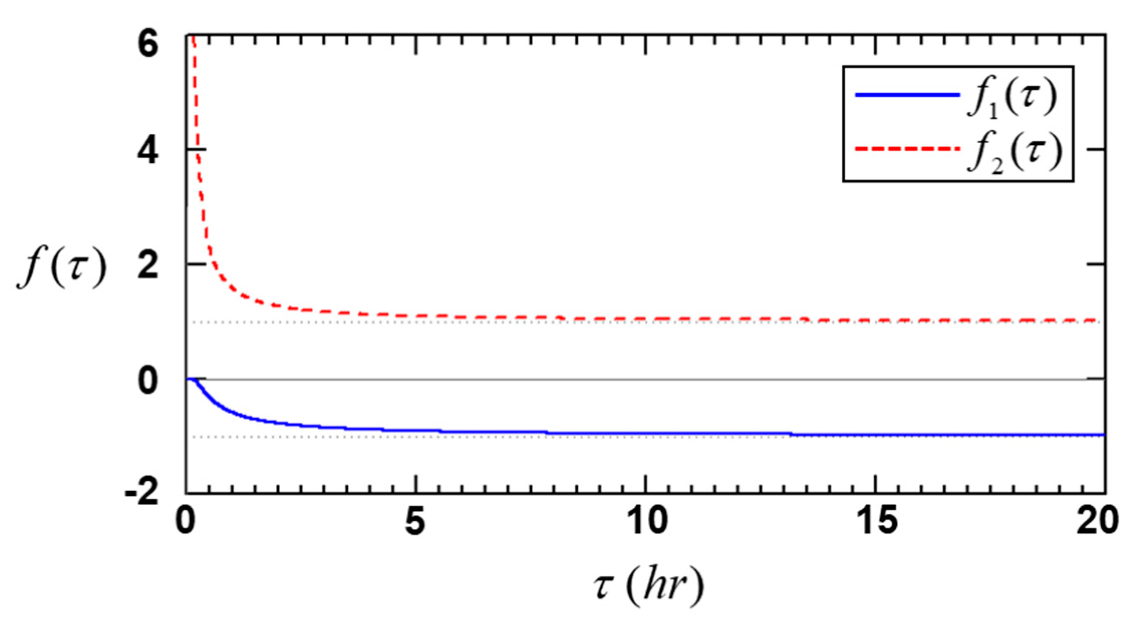
3.4.1. Determination of Lifetimes of Column NO_x (τ)

Determination of the lifetimes of column NO_x (τ) is an indispensable component in the estimation of top-down NO_x emissions. Many studies have conducted to estimate the NO_x lifetime [77,78,79,80]. Recently, Laughner and Cohen report that NO_x lifetime can be measured directly from satellite-observed NO₂ columns [79]. It is well-known that the chemical NO_x lifetimes are approximately several hours, depending on the latitudes and seasons [35,37]. The relatively short chemical NO_x lifetimes in summer are mainly characterized by the active NO_x chemical loss, leading to active HNO₃ formation via the reaction of NO₂ with OH radicals. The heterogeneous formation of nitrates through the N₂O₅ and NO₃ condensations onto aerosol surfaces is another important removal process of NO_x, particularly during winter. In the previous analysis of Han et al., the budget of NO_x chemical loss via the heterogeneous nitrate formation of N₂O₅ condensation (~49%) during winter was almost equivalent to that through the NO₂ + OH reactions over the Korean peninsula [81]. Besides, the formations of peroxyacetyl nitrates (PANs) and alkyl nitrates (ANs) are another important possible pathways related to NO_x chemical loss rates, and thus chemical lifetimes of NO_x [78,82,83].

In this study, we defined the lifetimes of NO_x columns (τ) as time how long columnar NO_x molecules persist at the given grid cell. The lifetime of NO_x columns was estimated from the mass balance equation with respect to the concentrations gradient of NO_x between the ith and i-1th time step, using several variables such as columnar NO_x (Ω_NOx), bottom-up NO_x emissions (E), and ΔQ from the CMAQ model simulations. For the calculation of τ, Equation (4) was rearranged from Equation (3). To find a root (i.e., τ) of this implicit nonlinear Equation (4), an approach based on the bisectional method was employed [84]. The mean values of τ in this study are 7.44 and 5.22 h over central-eastern China (covering Beijing, Tianjin, Hebei, Shanxi, Shandong, Henan, Jiangsu, Anhui, and Shanghai) in January and July, respectively. The values are slightly different to those from other studies [21,35,37]. For example, Martin et al. showed that the zonal mean lifetimes of NO_x over the 30–50 N° are ~10–~20 h in January and ~5 h in July [35]. While Martin et al. considered only the chemical loss of atmospheric NO_x via the oxidation to HNO₃ in the continental boundary layer for the calculation of NO_x lifetime (i.e., $\mathsf{\tau }=[\mathrm{N}{\mathrm{O}}_{\mathrm{x}}]/\left(k\left[\mathrm{O}\mathrm{H}\right]·\left[\mathrm{N}{\mathrm{O}}_2\right]\right)$), we employed entire fates of NO_x including transport in the current estimation of τ. In other words, current τ considers all the processes of NO_x such as chemical, physical, and meteorological removal from the given grid cells. Also, it should be noted that τ in the calculation covered only the time between 13:00 LT and 14:00 LT during the daytime. To more consistently compare chemical NO_x lifetimes with other studies, monthly chemical lifetimes of columnar NO_x without other effects (i.e., ΔQ = 0 in Equation (4)) should be employed. The average values of NO_x lifetime without other effects are 18.04 h and 8.29 h over central-eastern China and 15.12 h and 5.32 h over South Korea in January and July, respectively. The short (long) NO_x lifetimes in July (January) were possibly due to active NO_x chemical losses via OH + NO₂ reactions during summer and higher concentrations of NO_x during winter [85]. The lifetimes are closer to those of Martin et al.’s study. However, it should be stressed at this point that the NO_x lifetimes calculated with ΔQ = 0 are not exactly chemical NO_x lifetime, since they also include NO_x losses via dry and wet depositions.

Using the calculated τ and ΔQ, we investigated how successfully Equation (5) reproduces the bottom-up NO_x emissions (E_b). The reproduced NO_x emissions must be theoretically the same as the bottom-up NO_x emissions. As shown in Figure S2 in the supplementary materials, the recalculated values are almost equal to the bottom-up NO_x emissions. Their correlations (R²) and slopes (S) are close to 1.00, although some negative values are found overs the remote areas such as Russia, Mongolia, and the northwestern parts of China. Some negative values or small differences were caused mainly by truncation error in the bisectional calculations of τ. Mean errors (MEs) due to the uncertainty were estimated to be 0.05 × 10¹¹ and 0.02 × 10¹¹ molecules cm⁻² for January and July, respectively. The statistical analysis indicates that the total molecules of NO_x are conserved almost entirely in the mass balance approach.

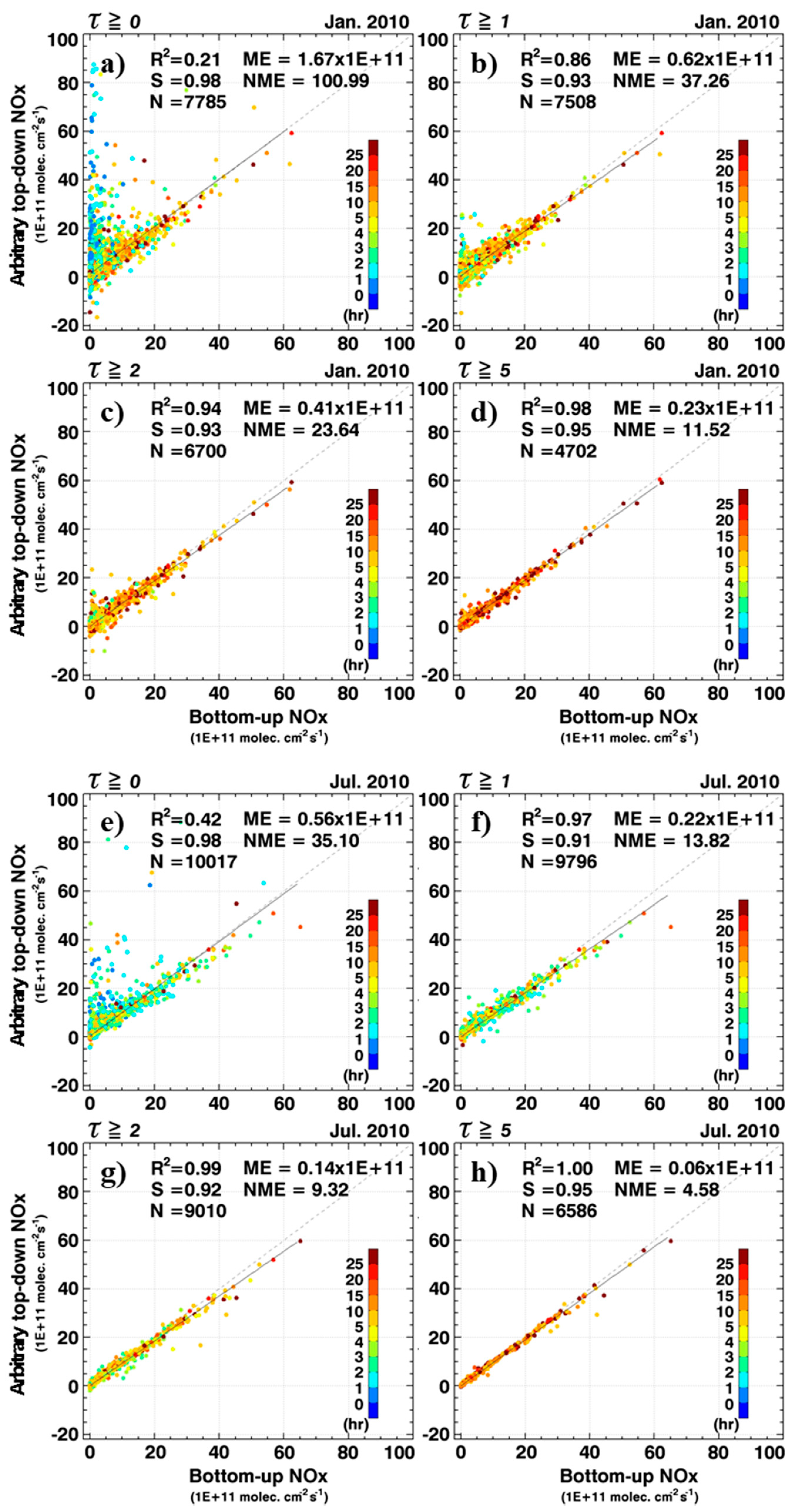
3.4.2. Sensitivity Analysis of τ

A small uncertainty in τ made a small impact on the estimation of top-down NO_x emissions over the remote continental regions in East Asia, as shown in Figure S2. However, top-down NO_x emissions can be highly uncertain when the small truncation error of τ is amplified with some errors caused by data interpolation. The interpolation of satellite data to model grid-cells inevitably produces some (small) errors, because the satellite-retrieved geophysical quantities do not accurately correspond to the model-gridded geophysical data [86]. To investigate such an impact on the estimation of the top-down NO_x emissions or non-linear Equation (5), we prepared satellite columnar NO_x (i.e., an arbitrary satellite data, Ω_NOx) on the OMI footprint based on the daily CMAQ-modeled NO_x columns. The daily satellite NO_x was then interpolated back to the model grid-cells. Finally, we put the interpolated satellite NO_x columns and other variables (i.e., τ and ΔQ) into Equation (5) to estimate the (arbitrary) top-down NO_x emissions (E_arb,t). It is expected that the arbitrary top-down NO_x emissions should, in theory, be the same as the bottom-up NO_x emissions (E_b), because the input data obtained directly from the CMAQ model simulations were used in this test. However, as shown in Figure S3, the E_arb,t was much larger than the E_b. These large overestimations of top-down NO_x emission were found, particularly over the low emissions areas of the bottom-up NO_x emissions (< ~10 × 10¹¹ molecules cm⁻² s⁻¹ in x-axis), as shown in the scatter plots in Figure S3.

To explore the unexpected overestimations of top-down NO_x emissions, the non-linear Equation (5) were analyzed in detail with respect to τ. Figure 3 presents a plot of the first and second terms on the right-hand side (f₁(τ) and f₂(τ)) of Equation (5), which are expressed by Equations (12) and (13), respectively. Equation (5) can be rearranged by Equation (14).

$$f_1(\mathsf{\tau })=\frac{e^{-1/\mathsf{\tau }}}{\mathsf{\tau }·\left(e^{-1/\mathsf{\tau }}-1\right)}$$

(12)

$$f_2(\mathsf{\tau })=\frac{-1}{\mathsf{\tau }·\left(e^{-1/\mathsf{\tau }}-1\right)}$$

(13)

$$\mathrm{E}={\mathsf{\Omega }}_{\mathrm{N}{\mathrm{O}}_{\mathrm{x},\mathrm{i}-1}}·f_1(\mathsf{\tau })+{\mathsf{\Omega }}_{\mathrm{N}{\mathrm{O}}_{\mathrm{x},\mathrm{i}}}·f_2(\mathsf{\tau })-\Delta \mathrm{Q}$$

(14)

Small changes in τ caused by truncation error in the bisectional method (discussed in Section 3.4.1) lead to a big difference in f₁(τ) and f₂(τ) around τ = 0–2 h in Figure 3, indicating that both the f₁(τ) and f₂(τ) can be highly uncertain around these ranges. The uncertain f₁(τ) and f₂(τ) are then multiplied by some error-involved Ω_NOx owing to the spatial interpolation (in Equation (14)). Eventually, the top-down NO_x emissions can be highly uncertain around τ = 0–2 h. The results were presented in scatter plot analysis between E_arb,t and E_b with respect to τ, as shown in Figure 4a,e).

Here, the color-coded circles represent τ at each grid cell. The large overestimations of E_arb,t were estimated, particularly around τ = 0–2 h due to the combined errors by τ and data interpolation, as explained. To minimize such impact on the top-down NO_x estimation, we filtered some data under the condition that τ is smaller than a specific value (i.e., 0, 1, 2, and 5 h) in Figure 4. This sensitivity test strongly indicates that the analysis can be influenced significantly by the data filtering of τ. For instance, when the data were filtered, the correlations (R²) generally improved from 0.21 to 0.98 for January (refer to more cases in Figures S4 and S5). Accordingly, mean errors (MEs) decreased from 1.67 × 10¹¹ to 0.23 × 10¹¹ molecules cm⁻² s⁻¹ (from 0.56 × 10¹¹ to 0.06 × 10¹¹ molecules cm⁻² s⁻¹) for January (July). Normalized mean errors also decreased, as shown in Figure 4. Furthermore, the slopes (S) were close to 1:1 line, 0.95 in the case of τ ≥ 5 h. However, less data (i.e., ‘N’ in Figure 4) was available for constructing the top-down NO_x emission.

Figure 5 showed the arbitrary top-down NO_x emissions (E_arb,t) and the differences between E_arb,t and E_b for the case of τ ≥ 5 h. As expected from Figure 4d,h, the spatial distributions and magnitudes of E_arb,t in Figure 5a,c were similar to those of E_b shown in Figure S2a,d. The ratios of the arbitrary top-down to the bottom-up NO_x emissions (${\mathrm{E}}_{\mathrm{v}\mathrm{i}\mathrm{r},\mathrm{t}}/{\mathrm{E}}_{\mathrm{b}}$) were approximately 1.02 and 1.00 for the entire domain in January and July, respectively. Also, the differences between E_arb,t and E_b were small and ranged mostly from ~–1 × 10¹¹ to ~1 × 10¹¹ molecules cm⁻² s⁻¹ for the entire domain (Figure 5b,d). In the seasonal perspective, data in July were denser than those in January for all the cases classified by the values of τ (Figure 4). More sparely scattered distributions in January were possibly caused by strong wind conditions in the cold seasons, as discussed in Section 3.3. From the sensitivity analysis, we, therefore, discarded some data showing τ smaller than two hours for the optimal estimation of the top-down NO_x emissions.

3.5. Satellite-Derived NO_x Columns

To apply the OMI-retrieved NO₂ columns to the top-down NO_x estimations, both OMI-derived NO_x columns at the ith and i-1th time steps are necessary for Equation (5). Since the OMI sensor does not provide the NO_x columns, but NO₂ columns only at the ith time step, two assumptions were made for the use of Equation (5). First, to convert OMI-retrieved NO₂ columns to the OMI-derived NO_x columns at the ith time step (${\mathsf{\Omega }}_{\mathrm{N}{\mathrm{O}}_{\mathrm{x}},\mathrm{O}\mathrm{M}\mathrm{I},\mathrm{i}}$), it was assumed that the ratios of NO_x columns to NO₂ columns in the CMAQ model simulations are the same with those in the OMI observations (Equation (15)), i.e.,:

$${\mathsf{\Omega }}_{\mathrm{N}{\mathrm{O}}_{\mathrm{x}},\mathrm{O}\mathrm{M}\mathrm{I},\mathrm{i}}={\mathsf{\Omega }}_{\mathrm{N}{\mathrm{O}}_2,\mathrm{O}\mathrm{M}\mathrm{I},\mathrm{i}}\times \frac{{\mathsf{\Omega }}_{\mathrm{N}{\mathrm{O}}_{\mathrm{x}},\mathrm{C}\mathrm{M}\mathrm{A}\mathrm{Q},\mathrm{i}}}{{\mathsf{\Omega }}_{\mathrm{N}{\mathrm{O}}_2,\mathrm{C}\mathrm{M}\mathrm{A}\mathrm{Q},\mathrm{i}}}$$

(15)

In this calculation, the averaging kernels (AKs) are also implicitly considered. Secondly, for the OMI-derived NO_x columns at the i-1th time step, it was assumed that the differences (ΔΩ_NOx,CMAQ) between the CMAQ-calculated NO_x columns at the ith and i-1th time steps were the same with those from the OMI observations (ΔΩ_NOx,OMI) as the following Equation (16):

$$\begin{array}{ll}{\mathsf{\Omega }}_{\mathrm{N}{\mathrm{O}}_{\mathrm{x}},\mathrm{O}\mathrm{M}\mathrm{I},\mathrm{i}-1}& ={\mathsf{\Omega }}_{\mathrm{N}{\mathrm{O}}_{\mathrm{x}},\mathrm{O}\mathrm{M}\mathrm{I},\mathrm{i}}+\left({\mathsf{\Omega }}_{\mathrm{N}{\mathrm{O}}_{\mathrm{x}},\mathrm{C}\mathrm{M}\mathrm{A}\mathrm{Q},\mathrm{i}-1}-{\mathsf{\Omega }}_{\mathrm{N}{\mathrm{O}}_{\mathrm{x}},\mathrm{C}\mathrm{M}\mathrm{A}\mathrm{Q},\mathrm{i}}\right)\\ & ={\mathsf{\Omega }}_{\mathrm{N}{\mathrm{O}}_{\mathrm{x}},\mathrm{O}\mathrm{M}\mathrm{I},\mathrm{i}}+\Delta {\mathsf{\Omega }}_{\mathrm{N}{\mathrm{O}}_{\mathrm{x}},\mathrm{C}\mathrm{M}\mathrm{A}\mathrm{Q}}\end{array}$$

(16)

$$\mathrm{E}=\frac{{\mathsf{\Omega }}_{\mathrm{N}{\mathrm{O}}_{\mathrm{x}},\mathrm{O}\mathrm{M}\mathrm{I},\mathrm{i}-1}·e^{-\Delta t/\mathsf{\tau }}-{\mathsf{\Omega }}_{\mathrm{N}{\mathrm{O}}_{\mathrm{x}},\mathrm{O}\mathrm{M}\mathrm{I},\mathrm{i}}}{\mathsf{\tau }·\left(e^{-\Delta t/\mathsf{\tau }}-1\right)}-\Delta \mathrm{Q}$$

(17)

The OMI-derived NO_x columns from the above calculations were finally applied to the top-down estimations of NO_x emissions (Equation (17)) over East Asia.

Shortly, the second assumption will not be necessary since the Korean geostationary environmental satellite of the Geostationary Korea Multi-Purpose Satellite/Geostationary Environmental Monitoring Spectrometer (GEOKOMPSAT/GEMS) provides us with hourly resolved ${\mathsf{\Omega }}_{\mathrm{N}{\mathrm{O}}_2}$ for Asia [87]. Also, this will be true for other geostationary satellite missions such as Sentinel 4 and TEMPO (Tropospheric Emissions: Monitoring of Pollution) over Europe and North America, respectively [88,89].

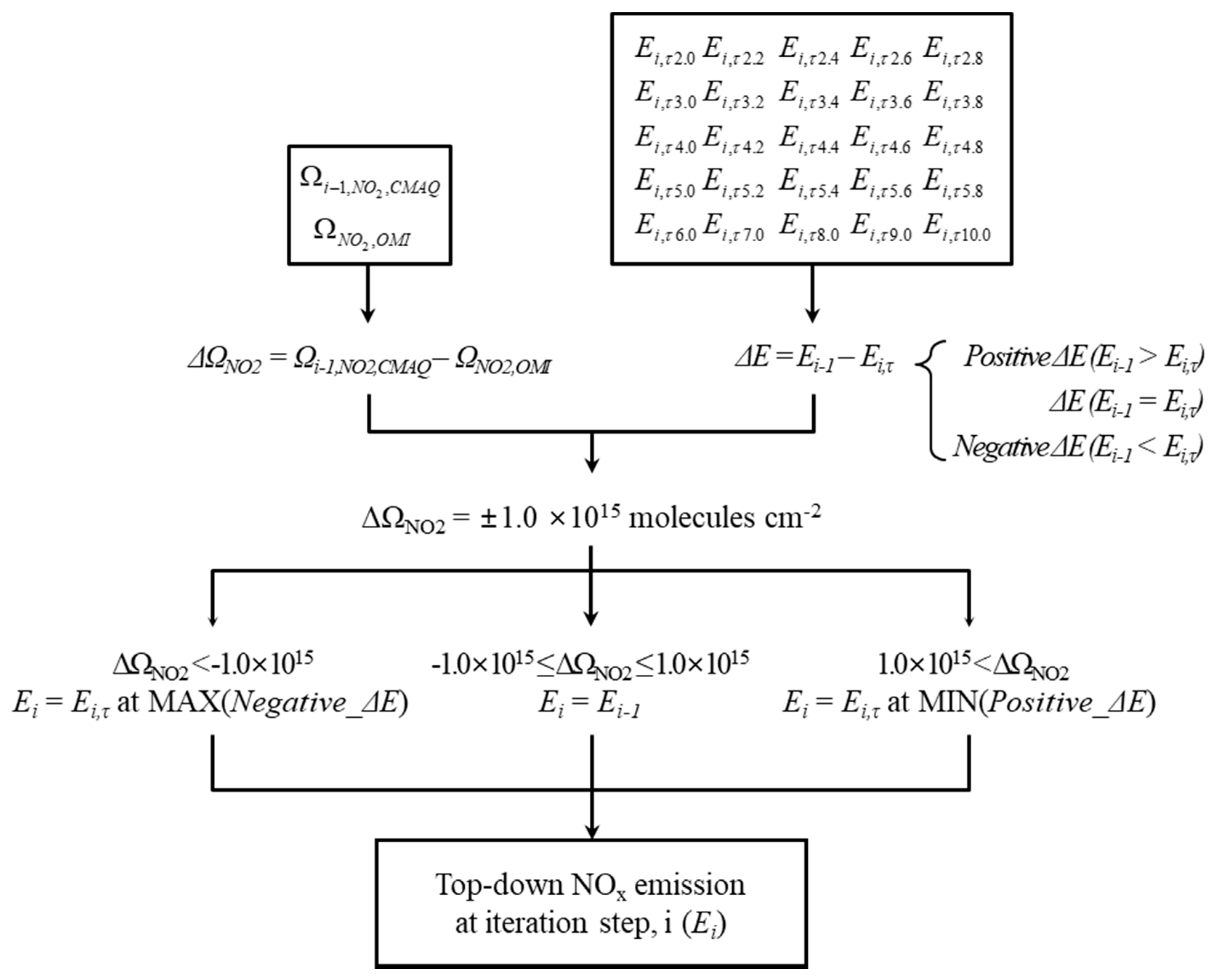
3.6. Optimal Conditions for the Top-Down NO_x Estimation

The OMI-retrieved data mentioned in Section 2.2 and Section 3.5 were utilized for the estimation of the top-down NO_x emissions over East Asia, using Equation (17). As shown in Figure 4, the top-down estimation of NO_x emissions showed generally acceptable results under the conditions of τ ≥ 2 h. However, to find optimal conditions at each grid cell, we prepared the 25 databases of the monthly top-down NO_x emissions (E_i,τ in Figure 6) at different conditions which are depending on τ. Despite conducting estimations of top-down NO_x emissions, some areas of the grid cells remain unoccupied (for example, white pixel areas in Figure 5). These white colors represented the areas where (i) OMI observations were not conducted during the periods because of large cloud fractions and/or high surface albedo, and/or (ii) τ shorter than the specific values were estimated. The unoccupied areas were then filled by spatial interpolation. Furthermore, the other remaining pixels after interpolations were replaced by the bottom-up NO_x emissions (i.e., E_i−1 in Figure 6) used in the previous CMAQ model simulations.

As shown in Figure 6, the optimal condition at each grid cell was then determined by combinations of ΔΩ_NO2 (= Ω_NO2,CMAQ − Ω_NO2,OMI) and ΔE (= E_i−1 − E_i,τ). Here, averaging kernels (AKs) were applied to the Ω_CMAQ for absolute differences. Also, the E_i−1 is the bottom-up NO_x emission (or top-down NO_x emission used in the previous CMAQ model simulation). Error tolerances are between −1.0 × 10¹⁵ and 1.0 × 10¹⁵ molecules cm⁻². Error tolerances are related to the uncertainties associated with the observation. Since the uncertainties in observations depend on the season and pixel, it should be applied differently to the algorithm. However, we fixed reference values to ±1.0 × 10¹⁵ molecules cm⁻² in this study because the error of the individual tropospheric NO₂ columns of the DOMINO v2.0 used in this application is ~1.0 × 10¹⁵ molecules cm⁻² [69]. For example, the top-down NO_x emission (E_i) at iteration step, i can be E_i−1 under the condition of 1.0 × 10¹⁵ > ΔΩ_NO2 > −1.0 × 10¹⁵ molecules cm⁻². If ΔΩ_NO2 is larger than 1.0 × 10¹⁵ molecules cm⁻², E_i should be reduced because NO_x emissions (E_i−1) utilized in the CMAQ simulations are overestimated. Therefore, E_i can be E_i,τ at the minimum case among the cases of positive ΔE (i.e., P_ΔE). In the case of ΔΩ_NO2 < −1.0 × 10¹⁵ molecules cm⁻², E_i can be E_i,τ at the maximum case, among the cases of negative ΔE (i.e., N_ΔE). Finally, estimated NO_x emissions were used in the next CMAQ model simulation to validate the NO_x emission fluxes and iterate the procedure.

4. Results and Discussions

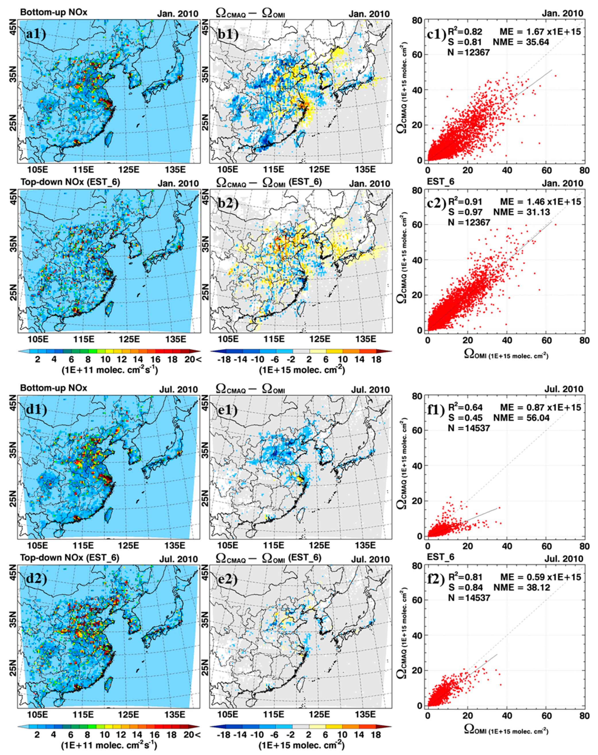
4.1. Comparison between Ω_NO2,CMAQ and Ω_NO2,OMI from Initial CMAQ Simulation

The NO₂ columns (Ω_NO2,CMAQ) calculated from the initial CMAQ simulation with the consideration of the bottom-up NO_x emission were compared with the OMI-retrieved NO₂ columns (Ω_NO2,OMI) over East Asia. For the sake of this comparison, the modeled concentrations of NO₂ at each layer were multiplied by the averaging kernels (AKs) from the KNMI/DOMINO products and were then vertically integrated from the surface to ~250 hPa for direct comparison between Ω_NO2,CMAQ and Ω_NO2,OMI. Figure 7(b1,c1,e1,f1) present the direct comparison for January and July. From the scatter plot analysis, the Ω_NO2,CMAQ were spatially well correlated to Ω_NO2,OMI with good correlation coefficients in January (R² = 0.82) and July (R² = 0.64). However, the absolute differences (ΔΩ_NO2 = Ω_NO2,CMAQ − Ω_NO2,OMI) showed large negative biases (i.e., bluish colors, approximate −0.8 × 10¹⁵ molecules cm⁻² over the entire domain) in both January and July over most regions of East Asia, except over some inland in January (e.g., Shanghai and Jiangsu province). For example, the absolute differences ranged approximately from −2 × 10¹⁵ to −1 × 10¹⁵ molecules cm⁻² over China, North Korea, South Korea, and Japan. In more detail, the highest absolute differences of −8.09 × 10¹⁵ and −8.02 × 10¹⁵ molecules cm⁻² were found over Beijing in January and Tianjin in July, respectively.

We also found the significant absolute differences ranging from −6 × 10¹⁵ to −3 × 10¹⁵ molecules cm⁻² over other regions such as Hebei, Shanxi, Guangdong, Shandong, and Hunan provinces. These negative biases (i.e., bluish colors) and some linear regression slopes less than unity (i.e., S < 1) in both January and July indicated that the bottom-up NO_x emission used in the initial simulations was possibly underestimated over most regions of East Asia. The bottom-up NO_x emissions used in the initial CMAQ simulations were 814 and 914 Gg N month⁻¹ over the entire domain for January and July, respectively.

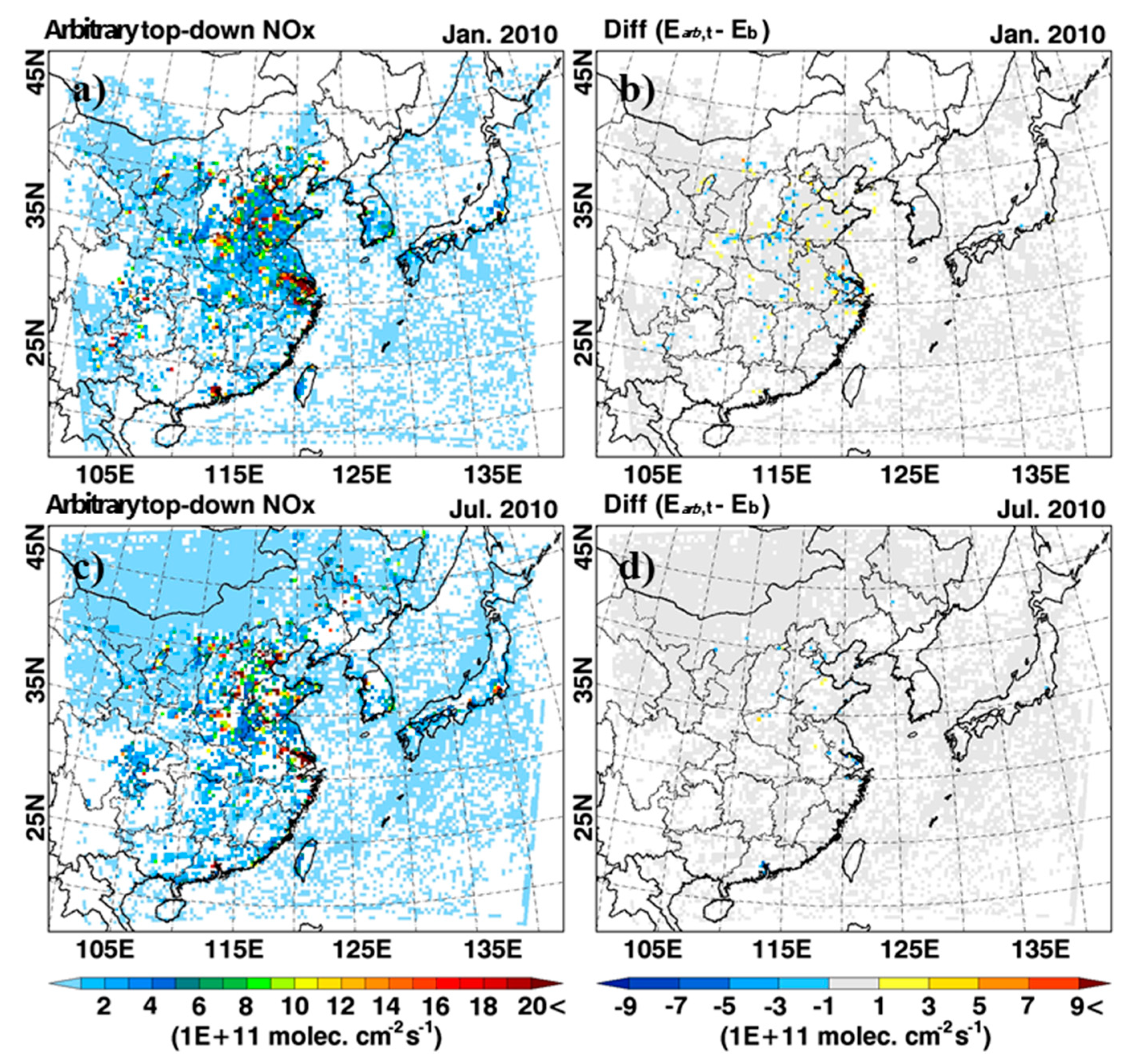
4.2. Top-Down NO_x Estimation and Comparisons between Ω_NO2,CMAQ and Ω_NO2,OMI

4.2.1. East Asia

To more accurately estimate NO_x emissions over East Asia, the estimation of the top-down NO_x emissions was conducted, using Equation (17) under the optimal condition described in Section 3.6. In this estimation, a six-iteration was performed for the final emission product, which presented in Figure 7(a2,d2) (refer to Figures S6 and S7 for all estimations). The spatial distributions of the top-down NO_x emissions were, in general, similar to those of the bottom-up NO_x emissions. For example, both the NO_x emissions showed high emission fluxes over central-eastern China (CEC) as well as in the megacities of Beijing, Shanghai, Hong Kong, Seoul, and Tokyo. Despite the spatial similarity, the top-down NO_x emissions were large by 19–34% in January and 19–47% in July over the entire domain, respectively, compared to the bottom-up NO_x emissions.

Table 2. Bottom-up and best top-down NO_x emission fluxes in China, North Korea, South Korea, Japan, and the entire domain.

Month	Region	Bottom-Up NOx	Best Top-Down NOx
Jan. (Gg N month−1)	Entire domain	814.20	990.99
	China	686.84	823.26
	N. Korea	6.29	8.16
	S. Korea	23.22	38.24
	Japan	41.26	50.11
Jul. (Gg N month−1)	Entire domain	913.55	1346.10
	China	780.72	1137.28
	N. Korea	6.71	12.95
	S. Korea	24.27	37.62
	Japan	36.07	63.41
Annual 1 (Tg N yr−1)	Entire domain	10.37	14.02
	China	8.81	11.76
	N. Korea	0.08	0.13
	S. Korea	0.28	0.46
	Japan	0.46	0.68

¹ Annual estimations was calculated linearly from the monthly top-down NO_x emissions both in January and July.

summarizes the top-down NO_x emission fluxes by country. The final estimates of the NO_x emissions over the entire domain were 991 Gg N month⁻¹ and 1346 Gg N month⁻¹ in January and July, respectively. As in the bottom-up NO_x emissions, the top-down NO_x emission fluxes in July were also larger than those in January because of possible contributions from soil microbiological activity during summer.

The direct comparisons between Ω_NO2,CMAQ and Ω_NO2,OMI were made in order to determine the optimal NO_x emissions for the next estimation and also to confirm how much the estimated top-down NO_x emissions were improved. Figure 7 presents the absolute differences and scatter plots between the two Ω_NO2 in the second and third columns, respectively (also, refer to Figures S6 and S7). According to the comparison analysis, there were significant improvements in the final estimation of the top-down NO_x emissions, in terms of the linear regression slopes, correlation coefficients, and absolute differences between Ω_NO2,CMAQ and Ω_NO2,OMI, during both January and July. For example, the linear regression slopes for the final estimation of the top-down NO_x emissions were close to the 1:1 line (S = 0.97 for January and 0.84 for July), compared to those for the initial simulations with the bottom-up NO_x emissions (S = 0.81 for January and 0.45 for July).

Also, the correlation coefficients (R²) increased from 0.82 to 0.88 in January and from 0.64 to 0.81 in July. Furthermore, absolute differences over the entire domain decreased from −0.83 × 10¹⁵ molecules cm⁻² to 0.31 × 10¹⁵ molecules cm⁻² in January, and from −0.82 × 10¹⁵ to −0.38 × 10¹⁵ molecules cm⁻² in July. We believe that there are marked improvements.

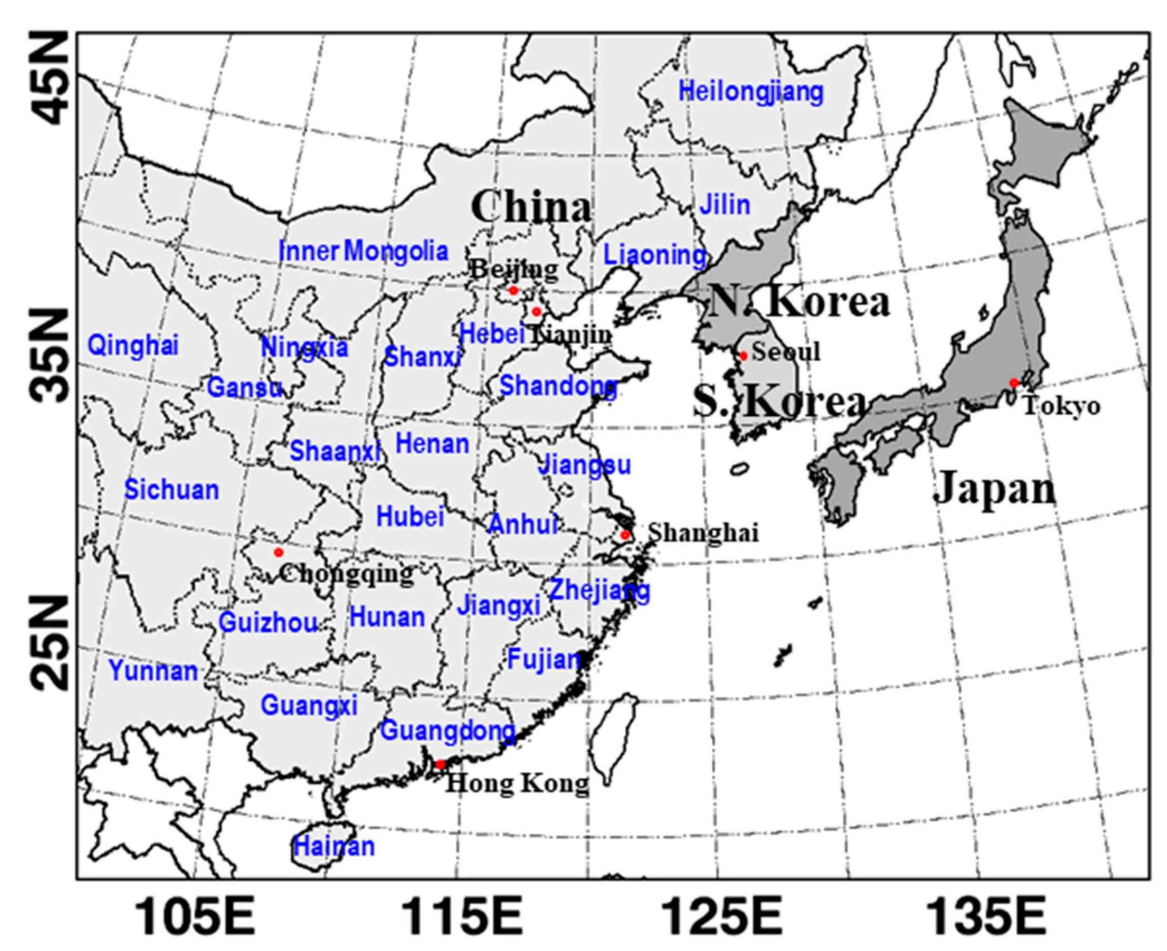
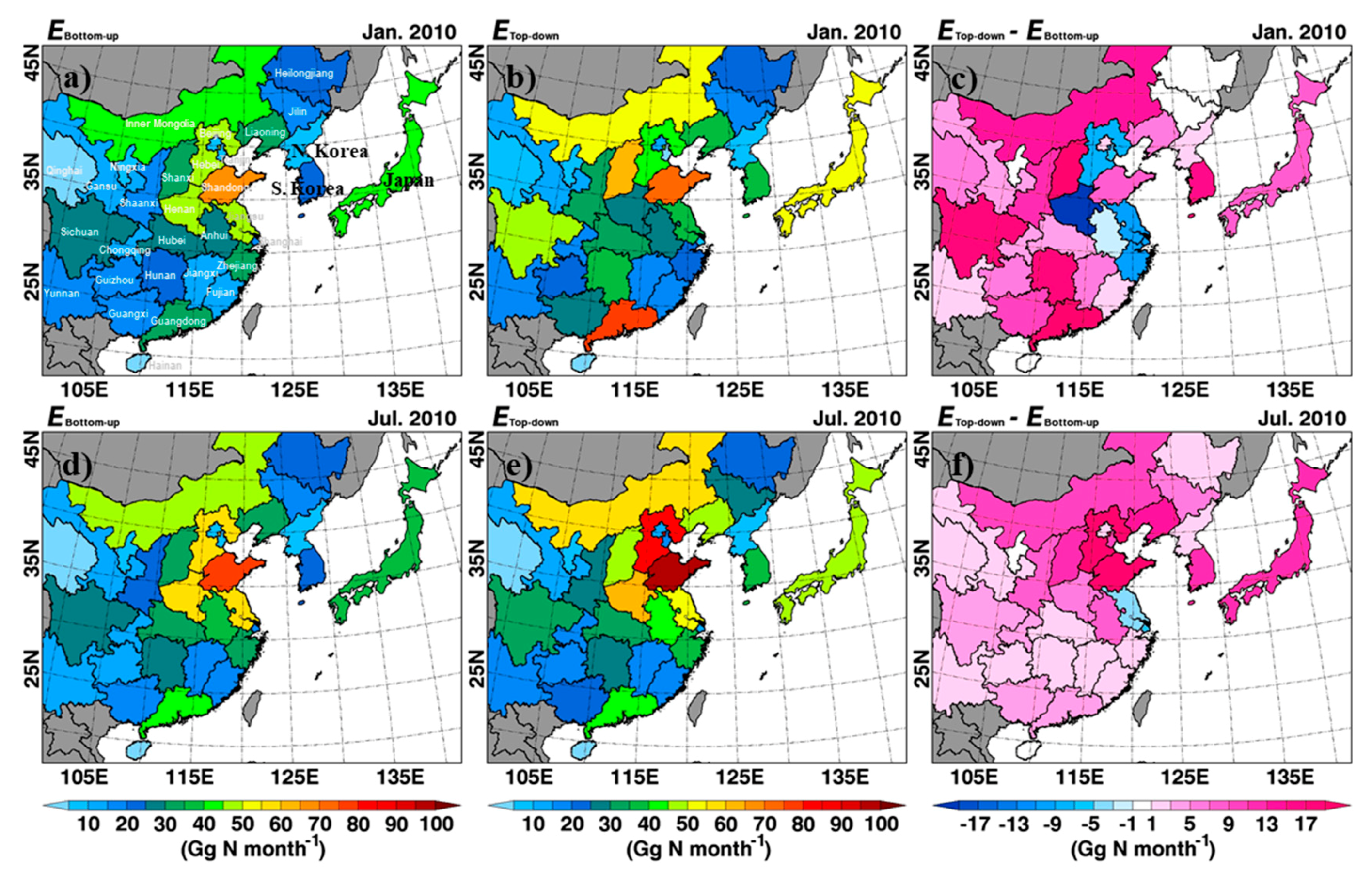
4.2.2. China, North Korea, South Korea, and Japan

For a more detailed analysis, we investigated the variations of the absolute differences (ΔΩ = Ω_CMAQ − Ω_OMI) after individual iteration over Chinese regions, North Korea, South Korea, and Japan, as shown in Figure 8. In January, variations were substantial after each iteration over several polluted regions such as Beijing, Tianjin, and Hebei, Henan, Shandong, Anhui, Jiangsu, and Shandong provinces. The fluctuations in ΔΩ over Beijing, Tianjin, and the Shanghai provinces were even higher than those over other regions, due to a relatively small number of pixels for the analysis. However, ΔΩ in January was reduced rapidly after the first iteration (also, refer to the second column of Figure S6). Eventually, the differences after the final (sixth) iteration were within the error tolerance of ±1.0 × 10¹⁵ molecules cm⁻² over most of the Chinese provinces. On the other hand, in July the variations of ΔΩ from the first to the sixth iterations were almost constant within the error tolerance over most of the Chinese provinces, except over Tianjin and Shanghai provinces, indicating that our estimations represent real NO_x emission fluxes over most of China with considerable accuracy.

For North Korea, positive biases in January were substantial at the third to fifth iterations (refer to Figure S6(b4–b6)). Those were mainly due to abnormally high NO_x emissions from a specific pixel over North Korea. Accordingly, in South Korea, the positive biases for the same period appear to be influenced by such NO_x plumes transported from North Korea (refer to Figure S6). The final estimation showed a slight overestimation over South Korea. In July, the absolute differences over North Korea and South Korea were getting close to zero. Over Japan, all the estimations showed good performances in January and July.

To validate the top-down NO_x estimation, it is also required to make a comparison using independent observation data. For the comparison, we used in-situ NO₂ measurement data for the Seoul metropolitan areas, which are quite densely distributed and only available open data for study periods. In South Korea, NO₂ measurements have been carried out using the commercial chemiluminescent detector. In the analyzer, ambient NO₂ passing through a molybdenum converter operating under 300–350 °C is converted to NO. However, other species like HNO₃ and PANs are converted together [90,91]. Nevertheless, we compared the CMAQ-calculated NO₂ data with in-situ NO₂ observation over Seoul Metropolitan areas. As shown in Figure S8 and

Table 3. Comparison between CMAQ-calculated and in-situ observed surface NO₂ concentration over the Seoul metropolitan areas.

Month	In-Situ	CMAQ w/Bottom-Up NOx	CMAQ w/Best Top-Down NOx
Jan. (ppb)	41.80 ± 10.91 *	24.05 ± 8.27	32.49 ± 13.19
Jul. (ppb)	23.78 ± 10.70	23.53 ± 8.18	22.43 ± 9.20

* mean concentration ± standard deviation for the 130 monitoring stations.

, the magnitudes of NO₂ calculated from the CMAQ simulation using the top-down emission is more close to the in-situ observation than those of CMAQ simulation with the bottom-up emissions, particularly in January.

More studies will be required for South Korea and some Chinese provinces such as Hebei and Shandong because they still have high biased pixels (refer to Figure 7(b2)). Even so, Table 2 showed the best top-down NO_x emissions estimated by the country. The annual estimation was calculated linearly from the monthly top-down NO_x emissions in both January and July. The best top-down NO_x emissions over China were 11.76 Tg N yr⁻¹. Some other studies estimated the top-down NO_x emissions over China at 10.9 Tg N yr⁻¹ for 2005–2006, 7.65 Tg N yr⁻¹ for 2006, and 7.48 Tg N yr⁻¹ for 2007 [20,37,92]. Our emission is close to those from Lamsal et al. [37]. These differences may be attributed to different periods, grid resolutions, methodologies, and chemical mechanisms in the CTM simulations [93]. In terms of the different time windows, Miyazaki et al. reported +0.73 Tg N yr⁻¹ of annual increase rate from 2008 to 2010 in top-down NO_x emissions over China [41]. Thus, we believed that considering the annual increase rate, our estimated NO_x emissions are much closer to the other estimates for China.

Our best estimates of top-down NO_x emissions over North Korea, South Korea, and Japan are 0.13, 0.46, and 0.68 Tg N yr⁻¹, which were approximately 62%, 60%, and 47% larger than the bottom-up NO_x emissions, respectively. The estimates of the top-down NO_x emissions over S. Korea and Japan in this study are close to the bottom-up emissions from EDGAR v4.3.2 [94], showing 0.45 Tg N yr⁻¹ and 0.64 Tg N yr⁻¹ of the bottom-up NO_x emissions from South Korea and Japan, respectively.

Figure 9 presents spatial distributions of the bottom-up and top-down NO_x emission fluxes and the differences between these two NO_x inventories by country and Chinese province. Figure 9c shows large increases in the top-down NO_x emissions found over the Guangdong, Shanxi, Sichuan, and Hunan provinces. On the other hand, top-down emissions are lower than the bottom-up NO_x emissions in January over central-eastern China (e.g., Tianjin, Hebei, Henan, Anhui, Jiangsu, Shanghai, and Zhejiang), indicating decreases in the top-down NO_x emissions by −6.8% to −56.7%, compared with the bottom-up NO_x emissions (also, refer to Table S1 for the detailed regional bottom-up and top-down NO_x emission fluxes and their differences). Considering possible underestimations of bottom-up NO_x emissions in Figure 7(b1), this is an unexpected decrease in the top-down NO_x emissions over the Tianjin, Hebei, Henan, and Anhui provinces. Despite the decreases, the CMAQ-calculated levels of NO₂ over central-eastern China were enhanced by NO₂ transported from adjacent provinces, such as Shanxi, Shaanxi, Inner Mongolia, and others where the top-down NO_x emissions increase, as shown in Figure 9c. Again, this indicates that the considerations of NO_x transport from/to adjacent cells can be a crucial factor in the fine-grid resolved top-down estimation, based on a mass balance approach because this type of detailed NO_x transport occurring over central-eastern China would not be shown in coarse grid-resolution. In July, an increase in the top-down NO_x emissions was found over most Chinese provinces, particularly over the Hebei and Shandong provinces (approximately 22–23 Gg N month⁻¹).

5. Summary and Conclusions

In this study, an algorithm for the estimation of top-down NO_x emissions in a horizontal resolution of 30 × 30 km² was developed based on the mass balance approach. Key components considered in this algorithm were (i) the estimation of NO_x molecules transported from/to adjacent cells, and (ii) the calculation of the lifetimes of column NO_x (τ). The wind vector estimated from WRF simulations was analyzed, as discussed in Section 3.2 and Section 3.3 to quantify the amounts of NO_x molecules. For the calculations of τ, an implicit nonlinear equation (Equation (4)) derived from the mass conservation equation (Equation (3)) was solved (Section 3.4.1). The mean values of τ calculated from the nonlinear equation are approximate seven and five hours over central-eastern China in January and in July, respectively. In Section 3.4.2, the top-down NO_x estimations were significantly influenced (or overestimated) by combined uncertainties from truncation error in the τ calculation and the interpolation of satellite data. The sensitivity test showed the improvements in the top-down NO_x estimation via filtering the data under the conditions that columnar NO_x lifetimes (τ) are smaller than two hours. The optimal estimation of top-down NO_x emissions at each grid cell was determined based on the combinations of differences in NO₂ columns (ΔΩ_NO2 = Ω_NO2,CMAQ − Ω_NO2,OMI) and NO_x emissions (ΔE = E_i−1 − E_i,τ). Then, the algorithm applied to estimate of the top-down NO_x emissions over East Asia in conjunction with OMI observations. In the estimation, a six-iteration was conducted to generate the best top-down NO_x emissions over East Asia.

To check all the procedures taken in this study (e.g., corrections, interpolation of satellite NO₂ data, and calculations of τ and ΔQ), direct comparisons between Ω_NO2,CMAQ and Ω_NO2,OMI were also made for January and July. The comparison analysis showed significant improvement over the CEC regions, particularly in January, when the final top-down NO_x emissions were used in the CMAQ model simulation. The absolute differences decreased from −0.83 × 10¹⁵ to 0.31 × 10¹⁵ molecules cm⁻² in January and from −0.82 × 10¹⁵ to −0.38 × 10¹⁵ molecules cm⁻² in July.

The best estimates of the top-down NO_x emissions were 11.76, 0.13, 0.46, and 0.68 Tg N yr⁻¹ over China, North Korea, South Korea, and Japan, which were large by 34%, 62%, 60%, and 47%, respectively. From the regional analysis in Chinese provinces, the best top-down NO_x emissions varied considerably according to regions and seasons. It was shown that for January, the best top-down NO_x emissions decreased, compared to the bottom-up NO_x emissions over the central-eastern China regions of Tianjin, Hebei, Henan, Jiangsu, Anhui, Shanghai, and Zhejiang. On the other hand, for July, the top-down NO_x emissions were large, compared to the bottom-up NO_x emissions, over most Chinese provinces. However, it should not be excluded that the top-down estimate in the study can underestimate the true value because of significant low biases in the current OMI-retrieved tropospheric NO₂ columns, compared with MAX-DOAS observations.

In the future, it is expected that the hourly top-down NO_x and SO₂ emissions for much finer grid resolution can be estimated with the currently developed algorithm, using the data from the geostationary satellite sensors, such as GEMS onboard GEO-KOMPSAT-2B over Asia, TEMPO onboard TEMPO over North America, and Sentinel-4 onboard Meteosat Third Generation-Sounder (MTG-S) over Europe [87,88,89]. Such efforts to retrieve the hourly concentrations of atmospheric pollutants via the data from geostationary satellite sensors, to estimate the emission fluxes, and to evaluate their accuracies, could improve the future performance of air quality modeling. For example, in using Equation (17), the previous concentrations (Ω_NOx,i−1) will no longer be obtained from the CTM simulations, but directly from GEO monitoring data. Therefore, after the successful launch of the GEO sensors, we will revisit this issue.

References

1. Chen, J.; Zhao, C.S.; Ma, N.; Liu, P.F.; Göbel, T.; Hallbauer, E.; Deng, Z.Z.; Ran, L.; Xu, W.Y.; Liang, Z.; et al. A parameterization of low visibilities for hazy days in the North China Plain. Atmos. Chem. Phys. 2012, 12, 4935–4950. [Google Scholar] [CrossRef] [Green Version]
2. Fu, G.Q.; Xu, W.Y.; Yang, R.F.; Li, J.B.; Zhao, C.S. The distribution and trends of fog and haze in the North China Plain over the past 30 years. Atmos. Chem. Phys. 2014, 14, 11949–11958. [Google Scholar] [CrossRef] [Green Version]
3. Zheng, G.J.; Duan, F.K.; Su, H.; Ma, Y.L.; Cheng, Y.; Zheng, B.; Zhang, Q.; Huang, T.; Kimoto, T.; Chang, D.; et al. Exploring the severe winter haze in Beijing: The impact of synoptic weather, regional transport and heterogeneous reactions. Atmos. Chem. Phys. 2015, 15, 2969–2983. [Google Scholar] [CrossRef] [Green Version]
4. Bytnerowicz, A.; Omasa, K.; Paoletti, E. Integrated effects of air pollution and climate change on forests: A northern hemisphere perspective. Environ. Pollut. 2007, 147, 438–445. [Google Scholar] [CrossRef]
5. United Nation Environment Program (UNEP). Forests suffer from air pollution. In Vital Forest Graphics; UNEP/GRID: Arendal, Norway, 2009; pp. 50–51. [Google Scholar]
6. Lelieveld, J.; Evans, J.S.; Fnais, M.; Giannadaki, D.; Pozzer, A. The contribution of outdoor air pollution sources to premature mortality on a global scale. Nature 2015, 525, 367–371. [Google Scholar] [CrossRef]
7. Hanna, S.R.; Chang, J.C.; Fernau, M.E. Monte Carlo estimates of uncertainties in predictions by a photochemical grid model (UAM-IV) due to uncertainties in input variables. Atmos. Environ. 1998, 32, 3619–3628. [Google Scholar] [CrossRef]
8. Zhang, Y.; Bocquet, M.; Mallet, V.; Seigneur, C.; Baklanov, A. Real-time air quality forecasting, part I: History, techniques, and current status. Atmos. Environ. 2012, 60, 632–655. [Google Scholar] [CrossRef]
9. Zhang, Y.; Bocquet, M.; Mallet, V.; Seigneur, C.; Baklanov, A. Real-time air quality forecasting, part II: State of the science, current research needs, and future prospects. Atmos. Environ. 2012, 60, 656–676. [Google Scholar] [CrossRef]
10. Streets, D.G.; Bond, T.C.; Carmichael, G.R.; Fernandes, S.D.; Fu, Q.; He, D.; Klimont, Z.; Nelson, S.M.; Tsai, N.Y.; Wang, M.Q.; et al. An inventory of gaseous and primary aerosol emissions in Asia in the year 2000. J. Geophys. Res. 2003, 108, 8809. [Google Scholar] [CrossRef]
11. Zhang, Q.; Streets, D.G.; He, K.; Wang, Y.; Richter, A.; Burrows, J.P.; Uno, I.; Jang, C.J.; Chen, D.; Yao, Z.; et al. NOx emission trends for China, 1995–2004: The view from the ground and the view from space. J. Geophys. Res. 2007, 112, D22306. [Google Scholar] [CrossRef] [Green Version]
12. Xing, J.; Wang, S.X.; Chatani, S.; Zhang, C.Y.; Wei, W.; Hao, J.M.; Klimont, Z.; Cofala, J.; Amann, M. Projections of air pollutant emissions and its impacts on regional air quality in China in 2020. Atmos. Chem. Phys. 2011, 11, 3119–3136. [Google Scholar] [CrossRef] [Green Version]
13. Zhao, Y.; Nielsen, C.P.; Lei, Y.; McElroy, M.B.; Hao, J. Quantifying the uncertainties of a bottom-up emission inventory of anthropogenic atmospheric pollutants in China. Atmos. Chem. Phys. 2011, 11, 2295–2308. [Google Scholar] [CrossRef] [Green Version]
14. Han, K.M.; Lee, S.; Chang, L.S.; Song, C.H. A comparison study between CMAQ-simulated and OMI-retrieved NO2 columns over East Asia for evaluation of NOx emission fluxes of INTEX-B, CAPSS, and REAS inventories. Atmos. Chem. Phys. 2015, 15, 1913–1938. [Google Scholar] [CrossRef] [Green Version]
15. Beirle, S.; Boersma, K.F.; Platt, U.; Lawrence, M.G.; Wagner, T. Megacity emissions and lifetimes of nitrogen oxides probed from space. Science 2011, 333, 1737–1739. [Google Scholar] [CrossRef] [PubMed]
16. de Foy, B.; Lu, Z.; Streets, D.G.; Lamsal, L.N.; Duncan, B.N. Estimates of power plant NOx emissions and lifetimes from OMI NO2 satellite retrievals. Atmos. Environ. 2015, 116, 1–11. [Google Scholar] [CrossRef]
17. Souri, A.H.; Choi, Y.; Pan, S.; Curci, G.; Nowlan, C.R.; Janz, S.J.; Kowalewski, M.G.; Liu, J.; Herman, J.G.; Weinheimer, A.J. First top-down estimates of anthropogenic NOx emissions using high-resolution airborne remote sensing observations. J. Geophys. Res. Atmos. 2018, 123, 3269–3284. [Google Scholar] [CrossRef]
18. Goldberg, D.; Lu, Z.; Oda, T.; Lamsal, L.; Liu, F.; Griffin, D.; McLinden, C.; Krotkov, N.A.; Duncan, B.; Streets, D. Exploiting OMI NO2 satellite observations to infer fossil-fuel CO2 emissions from U.S. megacities. Sci. Total Environ. 2019, 695, 133805. [Google Scholar] [CrossRef]
19. Beirle, S.; Borger, C.; Dörner, S.; Li, A.; Hu, Z.; Liu, F.; Wang, Y.; Wagner, T. Pinpointing nitrogen oxide emissions from space. Sci. Adv. 2019, 5, eaax9800. [Google Scholar] [CrossRef] [Green Version]
20. Zhao, C.; Wang, Y. Assimilated inversion of NOx emissions over East Asia using OMI NO2 column measurements. Geophys. Res. Lett. 2009, 36, L06805. [Google Scholar] [CrossRef] [Green Version]
21. Lin, J.-T.; McElroy, M.B.; Boersma, K.F. Constraint of anthropogenic NOx emissions in China from different sectors: A new methodology using multiple satellite retrievals. Atmos. Chem. Phys. 2010, 10, 63–78. [Google Scholar] [CrossRef] [Green Version]
22. Ghude, S.D.; Pfister, G.G.; Jena, C.; van der A, R.J.; Emmons, L.K.; Kumar, R. Satellite constraints of nitrogen oxide (NOx) emissions from India based on OMI observations and WRF-Chem simulations. Geophys. Res. Lett. 2013, 40, 423–428. [Google Scholar] [CrossRef]
23. Itahashi, S.; Yumimoto, K.; Kurokawa, J.; Morino, Y.; Nagashima, T.; Miyazaki, K.; Maki, T.; Ohara, T. Inverse estimation of NOx emissions over China and India 2005–2016; contrasting recent trends and future perspectives. Environ. Res. Lett. 2019, 14, 124020. [Google Scholar] [CrossRef] [Green Version]
24. Liu, F.; Beirle, S.; Zhang, Q.; van der A, R.J.; Zheng, B.; Tong, D.; He, K. NOx emission trends over Chinese cities estimated from OMI observations during 2005 to 2015. Atmos. Chem. Phys. 2017, 17, 9261–9275. [Google Scholar] [CrossRef] [PubMed] [Green Version]
25. Qu, Z.; Henze, D.K.; Capps, S.L.; Wang, Y.; Xu, X.; Wang, J.; Keller, M. Monthly top-down NOx emissions for China (2005–2012): A hybrid inversion method and trend analysis. J. Geophys. Res. Atmos. 2017, 122, 4600–4625. [Google Scholar] [CrossRef]
26. Goldberg, D.; Lu, Z.; Streets, D.G.; de Foy, B.; Griffin, D.; McLinden, C.; Lamsal, L.; Krotkov, N.; Eskes, H. Enhanced capabilities of TROPOMI NO2: Estimating NOx from North American cities and power plants. Environ. Sci. Technol. 2019, 53, 12594–12601. [Google Scholar] [CrossRef] [PubMed]
27. Konovalov, I.B.; Beekmann, M.; Burrows, J.P.; Richter, A. Satellite measurement based estimates of decadal changes in European nitrogen oxides emissions. Atmos. Chem. Phys. 2008, 8, 2623–2641. [Google Scholar] [CrossRef] [Green Version]
28. Vinken, G.C.M.; Boersma, K.F.; van Donkelaar, A.; Zhang, L. Constraints on ship NOx emissions in Europe using GEOS-Chem and OMI satellite NO2 observations. Atmos. Chem. Phys. 2014, 14, 1353–1369. [Google Scholar] [CrossRef] [Green Version]
29. Zyrichidou, I.; Koukouli, M.E.; Balis, D.; Markakis, K.; Poupkou, A.; Katragkou, E.; Kioutsioukis, I.; Melas, D.; Boersma, K.F.; van Roozendael, M. Identification of surface NOx emission sources on a regional scale using OMI NO2. Atmos. Environ. 2015, 101, 82–93. [Google Scholar] [CrossRef]
30. Boersma, K.F.; Jacob, D.J.; Bucsela, E.J.; Perring, A.E.; Dirksen, R.; van der A, R.J.; Yantosca, R.M.; Park, R.J.; Wenig, M.O.; Bertram, T.H.; et al. Validation of OMI tropospheric NO2 observations during INTEX-B and application to constrain NOx emissions over the eastern United States and Mexico. Atmos. Environ. 2008, 42, 4480–4497. [Google Scholar] [CrossRef] [Green Version]
31. Tang, W.; Cohan, D.S.; Lamsal, L.N.; Xiao, X.; Zhou, W. Inverse modeling of Texas NOx emissions using space-based and ground-based NO2 observations. Atmos. Chem. Phys. 2013, 13, 11005–11018. [Google Scholar] [CrossRef] [Green Version]
32. Lu, Z.; Streets, D.G.; de Foy, B.; Lamsal, L.N.; Duncan, B.N.; Xing, J. Emissions of nitrogen oxides from US urban areas: Estimation from Ozone Monitoring Instrument retrievals for 2005–2014. Atmos. Chem. Phys. 2015, 15, 10367–10383. [Google Scholar] [CrossRef] [Green Version]
33. Souri, A.H.; Choi, Y.; Jeon, W.; Li, X.; Pan, S.; Diao, L.; Westenbarger, D.A. Constraining NOx emissions using satellite NO2 measurements during 2013 DISCOVER-AQ campaign. Atmos. Environ. 2016, 131, 371–381. [Google Scholar] [CrossRef]
34. Goldberg, D.L.; Saide, P.E.; Lamsal, L.N.; de Foy, B.; Lu, Z.; Woo, J.-H.; Kim, Y.; Kim, J.; Gao, M.; Carmichael, G.; et al. A top-down assessment using OMI NO2 suggests an underestimate in the NOx emissions inventory in Seoul, South Korea, during KORUS-AQ. Atmos. Chem. Phys. 2019, 19, 1801–1818. [Google Scholar] [CrossRef] [Green Version]
35. Martin, R.V.; Jacob, D.J.; Chance, K.; Kurosu, T.P.; Palmer, P.I.; Evans, M.J. Global inventory of nitrogen oxide emissions constrained by space-based observations of NO2 columns. J. Geophys. Res. 2003, 108, 4537. [Google Scholar] [CrossRef] [Green Version]
36. Martin, R.V.; Sioris, C.E.; Chance, K.; Ryerson, T.B.; Bertram, T.H.; Wooldridge, P.J.; Cohen, R.C.; Neuman, J.A.; Swanson, A.; Flocke, F.M. Evaluation of space-based constraints on global nitrogen oxide emissions with regional aircraft measurements over and downwind of eastern North America. J. Geophys. Res. 2006, 111, D15308. [Google Scholar] [CrossRef] [Green Version]
37. Lamsal, L.N.; Martin, R.V.; van Donkelaar, A.; Celarier, E.A.; Bucsela, E.J.; Boersma, K.F.; Dirksen, R.; Luo, C.; Wang, Y. Indirect validation of tropospheric nitrogen dioxide retrieved from the OMI satellite instrument: Insight into the seasonal variation of nitrogen oxides at northern midlatitudes. J. Geophys. Res. 2010, 115, D05302. [Google Scholar] [CrossRef]
38. Lamsal, L.N.; Martin, R.V.; Padmanabhan, A.; van Donkelaar, A.; Zhang, Q.; Sioris, C.E.; Chance, K.; Kurosu, T.P.; Newchurch, M.J. Application of satellite observations for timely updates to global anthropogenic NOx emission inventories. Geophys. Res. Lett. 2011, 38, L05810. [Google Scholar] [CrossRef]
39. Miyazaki, K.; Eskes, H.J.; Sudo, K. Global NOx emission estimates derived from an assimilation of OMI tropospheric NO2 columns. Atmos. Chem. Phys. 2012, 12, 2263–2288. [Google Scholar] [CrossRef] [Green Version]
40. Lamsal, L.N.; Krotkov, N.A.; Celarier, E.A.; Swartz, W.H.; Pickering, K.E.; Bucsela, E.J.; Gleason, J.F.; Martin, R.V.; Philip, S.; Irie, H.; et al. Evaluation of OMI operational standard NO2 column retrievals using in situ and surface-based NO2 observations. Atmos. Chem. Phys. 2014, 14, 11587–11609. [Google Scholar] [CrossRef] [Green Version]
41. Miyazaki, K.; Eskes, H.; Sudo, K.; Boersma, K.F.; Bowman, K.; Kanaya, Y. Decadal changes in global surface NOx emissions from multi-constituent satellite data assimilation. Atmos. Chem. Phys. 2017, 17, 807–837. [Google Scholar] [CrossRef] [Green Version]
42. Cooper, M.; Martin, R.V.; Padmanabhan, A.; Henze, D. Comparing mass balance and adjoint methods for inverse modeling of nitrogen dioxide column for global nitrogen oxide emissions. J. Geophys. Res. Atmos. 2017, 122, 4718–4734. [Google Scholar] [CrossRef]
43. Kurokawa, J.; Yumimoto, K.; Uno, I.; Ohara, T. Adjoint inverse modeling of NOx emissions over eastern China using satellite observations of NO2 column densities. Atmos. Environ. 2007, 43, 1878–1887. [Google Scholar] [CrossRef]
44. Qu, Z.; Henze, D.K.; Theys, N.; Wang, J.; Wang, W. Hybrid mass balance/4D-Var joint inversion of NOx and SO2 emissions in East Asia. J. Geophys. Res. Atmos. 2019, 124, 8203–8224. [Google Scholar] [CrossRef] [PubMed]
45. Wang, Y.; Wang, J.; Xu, X.; Henze, D.K.; Qu, Z. Inverse modeling of SO2 and NOx emissions over China from multi-sensor satellite data: 1. formulation and sensitivity analysis. Atmos. Chem. Phys. Discuss. 2019. in review. [Google Scholar]
46. Mijling, B.; van der A, R.J. Using daily satellite observations to estimate emissions of short-lived air pollutants on a mesoscopic scale. J. Geophys. Res. Atmos. 2012, 117, D17302. [Google Scholar] [CrossRef]
47. Ding, J.; van der A, R.J.; Mijling, B.; Levelt, P.F.; Hao, N. NOx emission estimates during the 2014 Youth Olympic Games in Nanjing. Atmos. Chem. Phys. 2015, 15, 9399–9412. [Google Scholar] [CrossRef] [Green Version]
48. Leue, C.; Wenig, M.; Wagner, T.; Klimm, O.; Platt, U.; Jähne, B. Quantitative analysis of NOx emission from global ozone monitoring experiment satellite image sequences. J. Geophys. Res. 2001, 106, 5493–5505. [Google Scholar] [CrossRef] [Green Version]
49. Toenges-Schuller, N.; Stein, O.; Rohrer, F.; Wahner, A.; Richter, A.; Burrows, J.P.; Beirle, S.; Wagner, T.; Platt, U.; Elvidge, C.D. Global distribution pattern of anthropogenic nitrogen oxide emissions: Correlation analysis of satellite measurements and model calculations. J. Geophys. Res. 2006, 111, D05312. [Google Scholar] [CrossRef] [Green Version]
50. Skamarock, W.C.; Klemp, J.B.; Dudhia, J.; Gill, D.O.; Barker, D.M.; Duda, M.G.; Huang, X.Y.; Wang, W.; Powers, J.G. A Description of the Advanced Research WRF Version 3; NCAR Technical Note; National Center for Atmospheric Research (NCAR): Boulder, CO, USA, 2008; pp. 1–113.
51. Stauffer, D.R.; Seaman, N.L. Use of four-dimensional data assimilation in a limited-area mesoscale model. Part I: Experiments with synoptic-scale data. Mon. Wea. Rev. 1990, 118, 1250–1277. [Google Scholar] [CrossRef] [Green Version]
52. Stauffer, D.R.; Seaman, N.L. Multiscale four-dimensional data assimilation. J. Appl. Meteorol. 1994, 33, 416–434. [Google Scholar] [CrossRef] [Green Version]
53. Hong, S.Y.; Noh, Y.; Dudhia, J. A new vertical diffusion package with and explicit treatment of entrainment processes. Mon. Wea. Rev. 2006, 134, 2318–2341. [Google Scholar] [CrossRef] [Green Version]
54. Dudhia, J. Numerical study of convection observed during the winter monsoon experiment using a mesoscale two-dimensional model. J. Atmos. Sci. 1989, 46, 3077–3107. [Google Scholar] [CrossRef]
55. Mlawer, E.J.; Taubman, S.J.; Brown, P.D.; Iacono, M.J.; Clough, S.A. Radiative transfer for inhomogenous atmosphere: RRTM, a validated correlated-k model for the longwave. J. Geophys. Res. 1997, 102, 16663–16682. [Google Scholar] [CrossRef] [Green Version]
56. Kain, J.S. The Kain-Frisch convective parameterization: An update. J. Appl. Meteor. 2004, 43, 170–181. [Google Scholar] [CrossRef] [Green Version]
57. Byun, D.W.; Schere, K.L. Review of the governing equations, computational algorithm, and other components of the models-3 community multi-scale air quality (CMAQ) modeling system. Appl. Mech. Rev. 2006, 59, 51–77. [Google Scholar] [CrossRef]
58. Binkowski, F.S.; Roselle, S.J. Models-3 community multi-scale air quality (CMAQ) model aerosol components: 1. model description. J. Geophys. Res. 2003, 108, 4183. [Google Scholar] [CrossRef]
59. Carter, W.P.L. Implementation of the SAPRC-99 Chemical Mechanism into the Models-3 Framework; United States Environmental Protection Agency (US-EPA): Washington, DC, USA, 2000; pp. 1–101. [Google Scholar]
60. Han, K.M.; Park, R.S.; Kim, H.K.; Woo, J.H.; Kim, J.; Song, C.H. Uncertainty in biogenic isoprene emissions and its impacts on troposphric chemistry in East Asia. Sci. Total Environ. 2013, 463–464, 754–771. [Google Scholar] [CrossRef] [Green Version]
61. Li, M.; Zhang, Q.; Kurokawa, J.-I.; Woo, J.-H.; He, K.; Lu, Z.; Ohara, T.; Song, Y.; Streets, D.G.; Carmichael, G.R.; et al. MIX: A mosaic Asian anthropogenic emission inventory under the international collaboration framework of the MICS-Asia and HTAP. Atmos. Chem. Phys. 2017, 17, 935–963. [Google Scholar] [CrossRef] [Green Version]
62. Janssens-Maenhout, G.; Crippa, M.; Guizzardi, D.; Dentener, F.; Muntean, M.; Pouliot, G.; Keating, T.; Zhang, Q.; Kurokawa, J.; Wankmüller, R.; et al. HTAP_v2.2: A mosaic of regional and global emission grid maps for 2008 and 2010 to study hemispheric transport of air pollution. Atmos. Chem. Phys. 2015, 15, 11411–11432. [Google Scholar] [CrossRef] [Green Version]
63. Sindelarova, K.; Granier, C.; Bouarar, I.; Guenther, A.; Tilmes, S.; Stavrakou, T.; Müller, J.-F.; Kuhn, U.; Stefani, P.; Knorr, W. Global data set of biogenic VOC emissions calculated by the MEGAN model over the last 30 years. Atmos. Chem. Phys. 2014, 14, 9317–9341. [Google Scholar] [CrossRef] [Green Version]
64. Darmenov, A.; da Silva, A.M. The Quick Fire Emission Dataset (QFED)—Documentation of Versions 2.1, 2.2 and 2.4; National Aeronautics and Space Administration (NASA): Maryland, MD, USA, 2013; pp. 1–183.
65. Leung, F.Y.T.; Logan, J.A.; Park, R.; Hyer, E.; Kasischke, E.; Streets, D.; Yurganov, L. Impacts of enhanced biomass burning in the boreal forests in 1998 on tropospheric chemistry and the sensitivity of model results to the injection height of emissions. J. Geophys. Res. 2007, 112, D10313. [Google Scholar] [CrossRef] [Green Version]
66. Hyer, E.J.; Allen, D.J.; Kasischke, E.S. Examining injection properties of boreal forest fires using surface and satellite measurements of CO transport. J. Geophys. Res. 2007, 112, D18307. [Google Scholar] [CrossRef] [Green Version]
67. Kurokawa, J.; Ohara, T.; Morikawa, T.; Hanayama, S.; Janssens-Maenhout, G.; Fukui, T.; Kawashima, K.; Akimoto, H. Emissions of air pollutants and greenhouse gases over Asian regions during 2000–2008: Regional Emission inventory in ASia (REAS) version 2. Atmos. Chem. Phys. 2013, 13, 11019–11058. [Google Scholar] [CrossRef] [Green Version]
68. Boersma, K.F.; Braak, R.; van der A, R.J. Dutch OMI NO2 (DOMINO) Data Product v2.0 HE5 Data File User Mannual; Royal Netherlands Meteorological Institute (KNMI): De Bilt, The Netherlands, 2011; pp. 1–21. [Google Scholar]
69. Boersma, K.F.; Eskes, H.J.; Dirksen, R.J.; van der A, R.J.; Veefkind, J.P.; Stammes, P.; Huijnen, V.; Kleipool, Q.L.; Sneep, M.; Claas, J.; et al. An improved tropospheric NO2 column retrieval algorithm for the Ozone Monitoring Instrument. Atmos. Meas. Tech. 2011, 4, 1905–1928. [Google Scholar] [CrossRef] [Green Version]
70. Platt, U. Differential optial absorption spectroscopy (DOAS). Chem. Anal. Series 1994, 127, 27–83. [Google Scholar]
71. Dirksen, R.J.; Boersma, K.F.; Eskes, H.J.; Ionov, D.V.; Bucsela, E.J.; Levelt, P.F.; Kelder, H.M. Evaluation of stratospheric NO2 retrieved from the ozone monitoring instrument: Intercomparison, diurnal cycle and trending. J. Geophys. Res. 2011, 116, D08305. [Google Scholar] [CrossRef] [Green Version]
72. Irie, H.; Boersma, K.F.; Kanaya, Y.; Takashima, H.; Pan, X.; Wang, Z.F. Quantitative bias estimates for tropospheric NO2 columns retrieved from SCIAMACHY, OMI, and GOME-2 using a common standard for East Asia. Atmos. Meas. Tech. 2012, 5, 2403–2411. [Google Scholar] [CrossRef] [Green Version]
73. Ma, J.Z.; Beirle, S.; Jin, J.L.; Shaiganfar, R.; Yan, P.; Wagner, T. Tropospheric NO2 vertical column densities over Beijing: Results of the first three years of ground-based MAX-DOAS measurements (2008–2011) and satellite validation. Atmos. Chem. Phys. 2013, 13, 1547–1567. [Google Scholar] [CrossRef] [Green Version]
74. McLinden, C.A.; Fioletov, V.; Boersma, K.F.; Kharol, S.K.; Krotkov, N.; Lamsal, L.; Makar, P.A.; Martin, R.V.; Veefkind, J.P.; Yang, K. Improved satellite retrievals of NO2 and SO2 over the Canadian oil sands and comparisons with surface measurements. Atmos. Chem. Phys. 2014, 14, 3637–3656. [Google Scholar] [CrossRef] [Green Version]
75. Drosoglou, T.; Bais, A.F.; Zyrichidou, I.; Kouremeti, N.; Poupkou, A.; Liora, N.; Giannaros, C.; Koukouli, M.E.; Balis, D.; Melas, D. Comparisons of ground-based tropospheric NO2 MAX-DOAS measurements to satellite observations with the aid of an air quality model over the Thessaloniki area, Greece. Atmos. Chem. Phys. 2017, 17, 5829–5849. [Google Scholar] [CrossRef] [Green Version]
76. Mak, H.W.L.; Laughner, J.L.; Fung, J.C.H.; Zhu, Q.; Cohen, R.C. Improved satellite retrieval of tropospheric NO2 column density via updating of air mass factor (AMF): Case study of Southern China. Remote Sens. 2018, 10, 1789. [Google Scholar] [CrossRef] [Green Version]
77. Liu, F.; Beirle, S.; Zhang, Q.; Dörner, S.; He, K.; Wagner, T. NOx lifetimes and emissions of cities and power plants in polluted background estimated by satellite observations. Atmos. Chem. Phys. 2016, 16, 5283–5298. [Google Scholar] [CrossRef] [Green Version]
78. Kenagy, H.S.; Sparks, T.L.; Ebben, C.J.; Wooldrige, P.J.; Lopez-Hilfiker, F.D.; Lee, B.H.; Thornton, J.A.; McDuffie, E.E.; Fibiger, D.L.; Brown, S.S.; et al. NOx lifetime and NOy partitioning during WINTER. J. Geophys. Res. 2018, 123, 9813–9827. [Google Scholar]
79. Laughner, J.; Cohen, R.C. Direct observation of changing NOx lifetime in North America cities. Science 2019, 366, 723–727. [Google Scholar] [CrossRef] [PubMed]
80. Shah, V.; Jacob, D.J.; Li, K.; Silvern, R.F.; Zhai, S.; Liu, M.; Lin, J.; Zhang, Q. Effect of changing NOx lifetime on the seasonality and long-term trends of satellite-observed tropospheric NO2 columns over China. Atmos. Chem. Phys. 2020, 20, 1483–1495. [Google Scholar] [CrossRef] [Green Version]
81. Han, K.M.; Song, C.H. A budget analysis of NOx column losses over the Korean peninsula. Asia Pac. J. Atmos. Sci. 2012, 48, 55–65. [Google Scholar] [CrossRef]
82. Browne, E.C.; Cohen, R.C. Effects of biogenic nitrate chemistry on the NOx lifetime in remote continental regions. Atmos. Chem. Phys. 2012, 12, 11917–11932. [Google Scholar] [CrossRef] [Green Version]
83. Han, K.M.; Lee, S.; Yoon, Y.J.; Lee, B.Y.; Song, C.H. A model investigation into the atmospheric NOy chemistry in remote continental Asia. Atmos. Environ. 2019, 214, 116817. [Google Scholar] [CrossRef]
84. Heath, M.T. Scientific Computing: An Introductory Survey, 2nd ed.; McGraw-Hill: New York, NY, USA, 2002; pp. 1–563. [Google Scholar]
85. Valin, L.C.; Russell, A.R.; Hudman, R.C.; Cohen, R.C. Effects of model resolution on the interpretation of satellite NO2 observations. Atmos. Chem. Phys. 2011, 11, 11647–11655. [Google Scholar] [CrossRef] [Green Version]
86. Boersma, K.F.; Vinken, G.C.M.; Eskes, H.J. Representativeness errors in comparing chemistry transport and chemistry climate models with satellite UV/Vis tropospheric column retrievals. Geosci. Model Dev. 2016, 9, 875–898. [Google Scholar] [CrossRef] [Green Version]
87. Kim, J.; Jeong, U.; Ahn, M.; Kim, J.H.; Park, R.J.; Lee, H.; Song, C.H.; Choi, Y.S.; Lee, K.H.; Yoo, J.M.; et al. New era of air quality monitoring from space: Geostationary environment monitoring spectrometer (GEMS). Bull. Amer. Meteor. Soc. 2020, 101, E1–E22. [Google Scholar] [CrossRef] [Green Version]
88. Chance, K.; Lui, X.; Suleiman, R.M.; Flittner, D.E.; Janz, S.J. Tropspheric emissions: Monitoring of pollution (TEMPO). In Proceedings of the AGU Fall Meeting, San Francisco, CA, USA, 3–7 December 2012. [Google Scholar]
89. Ingmann, P.; Veihelmann, B.; Langen, J.; Lamarre, D.; Stark, H.; Courreges-Lacoste, G.B. Requirements for the GMES atmosphere service and ESA’s implementation concept: Sentinels-4/-5 and-5p. Remote Sens. Environ. 2012, 120, 58–69. [Google Scholar] [CrossRef]
90. Lamsal, L.N.; Duncan, B.N.; Yoshida, Y.; Krotkov, N.U.S. NO2 trends (2005–2013): EPA air quality system (AQS) data versus improved observations from the ozone monitoring instrument (OMI). Atmos. Environ. 2015, 110, 130–143. [Google Scholar] [CrossRef]
91. Dunlea, E.J.; Herndon, S.C.; Nelson, D.D.; Volkamer, R.M.; San Martini, F.; Sheehy, P.M.; Zahniser, M.S.; Shorter, J.H.; Wormhoudt, J.; Lamb, B.K.; et al. Evaluation of nitrogen dioxide chemiluminescence monitors in a polluted urban environment. Atmos. Chem. Phys. 2007, 7, 2691–2704. [Google Scholar] [CrossRef] [Green Version]
92. Lin, J.-T. Satellite constraint for emissions of nitrogen oxides from anthropogenic, lightning and soil sources over East China on a high-resolution grid. Atmos. Chem. Phys. 2012, 12, 2881–2898. [Google Scholar] [CrossRef] [Green Version]
93. Lin, J.-T.; Liu, Z.; Zhang, Q.; Liu, H.; Mao, J.; Zhuang, G. Modeling uncertainties for tropospheric nitrogen dioxide columns affecting satellite-based inverse modeling of nitrogen oxides emissions. Atmos. Chem. Phys. 2012, 12, 12255–12275. [Google Scholar] [CrossRef]
94. Crippa, M.; Guizzardi, D.; Muntean, M.; Schaaf, E.; Dentener, F.; van Aardenne, J.A.; Monni, S.; Doering, U.; Olivier, J.G.J.; Pagliari, V.; et al. Gridded emissions of air pollutants for the period 1970–2012 within EDGAR v4.3.2. Earth Syst. Sci. Data 2018, 10, 1987–2013. [Google Scholar] [CrossRef] [Green Version]
Figure 1. Modeling domain with political borders. Gray shaded regions in China, North Korea, South Korea, and Japan were selected for detailed analysis.
Remotesensing 12 02004 g001
Figure 2. Schematics for calculating the amounts of NOx molecules: (a) transported from an adjacent (black bashed) cell into a given (red dashed) cell (Qin); and (b) transported from a given (red dashed) cell into an adjacent cell (Qout).
Remotesensing 12 02004 g002
Figure 3. Plots of Equation (12) in blue line and Equation (13) in red dashed line.
Remotesensing 12 02004 g003
Figure 4. Scatter plots between bottom-up (Eb) and top-down NOx emissions (Et). (a,e) Et vs. Eb with τ ≥ 0 for January and July, respectively; (b,f) Et vs. Eb with τ ≥ 1 for January and July, respectively; (c,g) Et vs. Eb with τ ≥ 2 for January and July, respectively; (d,h) Et vs. Eb with τ ≥ 5 for January and July, respectively (unit: 1011 molecules cm−2 s−1).
Remotesensing 12 02004 g004
Figure 5. Spatial distributions of the top-down NOx emissions for the case of τ ≥ 5 in (a) January and (c) July and the differences between the top-down and bottom-up NOx emissions in (b) January and (d) July (unit: 1011 molecules cm−2 s−1).
Remotesensing 12 02004 g005
Figure 6. Schematics of the optical condition determined by combinations of ΔΩNO2 and ΔE.
Remotesensing 12 02004 g006
Figure 7. Spatial distributions of the NOx emissions (unit: 1011 molecules cm−2 s−1), differences between ΩCMAQ and ΩOMI (ΔΩ = ΩCMAQ − ΩOMI, unit: 1015 molecules cm−2), and scatter plots between ΩCMAQ and ΩOMI over East Asia for January and July are presented in the first, second, and third columns, respectively. (a1,d1) Bottom-up NOx emission. (a2,d2) Top-down NOx emissions by final iteration, respectively. (b1,e1) ΔΩ with the use of bottom-up NOx emission in the CMAQ simulation. (b2,e2) ΔΩ with the use of top-down NOx emissions in the CMAQ simulations. (c1) scatter plot with the use of bottom-up NOx emission in the CMAQ simulation. (c2,f2) scatter plots with the use of top-down NOx emissions in the CMAQ simulations. The R2, S, N, ME, and NME indicate the correlation coefficient, slope, number of available data, mean error (unit: 1011 molecules cm−2 s−1), and normalized mean error (unit: %), respectively.
Remotesensing 12 02004 g007
Figure 8. Variations of the absolute difference between ΩCMAQ and ΩOMI (ΔΩ = ΩCMAQ − ΩOMI) by iterations over Chinese provinces, North Korea, South Korea, and Japan by iterations (unit: 1015 molecules cm−2). Regions are defined in Figure 1.
Remotesensing 12 02004 g008
Figure 9. Spatial maps of Ebottom-up, Etop-down, and their differences (ΔE = Etop-down − Ebottom-up) by region (unit: Gg N month−1). (a,d) Ebottom-up for January and July, respectively. (b,e) Etop-down for January and July, respectively. (c,f) ΔE for January and July, respectively.
Remotesensing 12 02004 g009