Abstract
We investigate the applicability of offshore geoelectrical profiling in the littoral zone, e.g., for archaeological prospection, sediment classification and investigations on coastal ground water upwelling. We performed field measurements with a 20 m long multi-electrode streamer in inverse Schlumberger configuration, which we used to statistically evaluate measurement uncertainty and the reproducibility of offshore electric resistivity tomography. We compared floating and submerged electrodes, as well as stationary and towed measurements. We found out that apparent resistivity values can be determined with an accuracy of 1% to 5% (1σ) depending on the measurement setup under field conditions. Based on these values and focusing on typical meter-scale targets, we used synthetic resistivity models to theoretically investigate the tomographic resolution and depth penetration achievable near-beach underneath a column of brackish water of about 1 m depth. From the analysis, we conclude that offshore geoelectric sounding allows the mapping of archaeological stone settings. The material differentiation of low-porosity rock masses < 15% is critical. Submerged wooden objects show a significant resistivity contrast to sand and rocks. Distinguishing brine-saturated sandy sediments from cohesive silty-clayey sediments is difficult due to their equal or reversed resistivity contrasts. Submarine freshwater discharges in sandy aquifers can be localized well, though difficulties may occur if the seafloor encounters massive low-porosity rock masses. As to the measurement setups, submerged and floating electrodes differ in their spatial resolution. Whereas stone settings of 0.5 to 1 m can still be located with submerged electrodes within the uppermost 4 m underneath the seafloor, they have to be >2 m if floating electrodes are used. Therefore, we recommend using submerged electrodes, especially in archaeological prospection. Littoral geological and hydrogeological mapping is also feasible with floating electrodes in a more time-saving way.
1. Introduction
In recent years, various research issues in shallow water environments were investigated by marine electrical resistivity tomography (ERT). The method is sensitive to lateral and vertical changes in the subsurface electric resistivity and can be used to address materials, especially in extremely shallow water and gassy environments. Investigations include issues such as local groundwater upwelling in coastal areas [1] and geological variations of the subsoil [2,3] as well as meter-scale investigations prospecting archaeological objects, such as wall fundaments or ancient harbor installations [4,5]. In a shallow water environment, geoelectric measurements can be performed under excellent coupling conditions due to low water resistivity values and uniformly good contact of the electrodes to the medium. This allows stationary measurements as well as continuously towed measurements. Towed measurements show a faster and denser measurement coverage and therefore enable the survey of larger areas in less time than stationary measurements, whilst the positioning of the measurements is more imprecise [6]. However, the main limitation of the method also results from the low apparent resistivity values of the water, which is reducing the depth penetration [7].
Several studies investigated different aspects concerning the applicability of marine geoelectrical measurements for different measurement configurations and setups regarding the resolution. Simyrdanis et al compare inversion results of synthetic two-dimensional (2D) data for isolated underwater wall fundaments in a homogenous subsurface below a salty water column at 0.5 to 2 m water depth [8]. They differ between a Dipole–Dipole, Schlumberger and Pole–Dipole configuration as well as between submerged and floating electrodes. They recommend a Pole–Dipole or Schlumberger configuration and did not notice any difference for submerged and floating electrodes up to 1 m water depth. According to the study, objects have to be twice as wide as the electrode spacing to be resolved properly. A priori information, especially about the water depth, improves the results. However, incorrect a priori information can easily falsify the results. The authors of Reference [9] compare one-dimensional (1D) vertical electric sounding (VES) curves of floating and submerged electrodes for a three-layer case for both Schlumberger and Dipole–Dipole configuration. A higher contrast of the middle layer to its surrounding can be resolved with both setups and configurations more easily, no matter whether the resistivity values are larger or smaller than the surrounding. For small resistivity contrasts, the most feasible setup or configuration changes. Additionally, the study shows VES curves of a Wenner α configuration submerged to the bottom of an approximated shallow water two-layer case, with a maximum sub-bottom resistivity of 10 Ωm. For streamer lengths < 20 m and sub-bottom resistivity values > 7 Ωm, small uncertainties of the apparent resistivity can induce errors estimating the sub-bottom resistivity. VES curves approximating shallow water two-layer cases are also presented in Reference [10] for a Dipole–Dipole configuration. This study also considers that a streamer length > 20 m is required in order to be able to resolve resistivity values > 7 Ωm in the subsurface, but this in turn influences the spatial resolution. A study to overcome the limitations of deeper water (~50 m) is presented in Reference [11], designing a “fishing rod streamer” which is a vertical Pole–Pole configuration. Mansoor et al calculated sensitivity kernels for various electrode configurations in a homogenous subsurface, e.g., a modified Wenner α configuration, which is preferable to a Dipole–Dipole configuration regarding depth penetration [12]. They estimated measurement uncertainties by calculating the relative standard deviation of tie points in the measured profiles that include the forward and backward directions. A mean average uncertainty of 3.5% was observed.
Based on all this background, the presented study provides, for the first time, an integrated analysis of all field measurement uncertainty, theoretical spatial resolution of vertical sounding curves and two-dimensional (2D) profiles for two- and three/four-layer geology models, as well as sensitivity analyses for different measurement setups of a marine geoelectric system. We examine the ability of different measurement setups (mobile vs. stationary and floating vs. submerged electrodes) of a multi-electrode streamer of inverse Schlumberger configuration to reconstruct shallow water submarine stratigraphy. This includes:
- (i)
- Repeated measurements of parallel near-shore profiles in about 1 m water depth in different measurement setups to obtain a dataset that enables the statistical inquiry of measurement uncertainties and inversion reproducibility.
- (ii)
- Theoretical considerations based on forward modelling and inverse modelling to estimate the spatial resolution and depth penetration in 1D and 2D resistivity model data.
Following the studies of References [8] and [9], we use field measurement uncertainties to investigate the spatial resolution from layer resistivity and thickness from 1D forward modelling and inversion for different layer models. We provide information about the required streamer length and the depth resolution of layers. Furthermore, the 2D spatial resolution of multiple non-isolated objects below a water column are also considered. The paper starts with the investigation of the measurement accuracy and inversion reproducibility of field data before focusing on synthetic data to investigate the resolution and depth penetration for 1D cases, followed by the investigation of the spatial resolution of a 2D case.
2. Materials and Methods
2.1. Measurement Configurations, Field Measurements and Investigated Materials
To investigate the applicability of geoelectrical measurements in shallow water environments, a 20 m long multi-electrode streamer was used on test profiles conducted parallel to the Baltic Sea coastline. Due to its short length, it is easy to handle with two persons in about 1 m water depth without using a boat. An inverse Schlumberger configuration was used. The current electrodes C1 and C2 are positioned in the middle of the streamer and the potential electrodes P1a–P1b to P8a–P8b are symmetrically spaced to the sides around the streamer midpoint (Table 1, Figure 1a). This enables simultaneous measurements on all potential electrode pairs during current injection, meaning that one complete sounding curve of apparent electric resistivity is recorded during each measurement cycle. The sounding was performed with RESECS (Resistivity Electrode Control System) multi-channel geoelectric unit [13] and stainless-steel electrodes (see also Figure 2b). All equipment was manufactured by the company GeoServe in Kiel, Germany.

Table 1.
Inverse Schlumberger configuration used for Eckernförde repetition measurements.
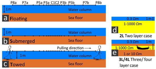
Figure 1.
Left column: Schematic view of different measurement setups including (a) stationary floating electrodes (setup F), (b) stationary submerged electrodes (setup S) and (c) towed floating electrodes (setup T). Right column: Images of (d) two-layer (2L), and (e) three-layer cases (3L), approximating meter-scale targets. “C” indicates the current electrodes and “P” the potential electrodes of the streamer.
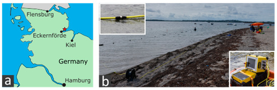
Figure 2.
(a) Location of Eckernförde Bay in Germany, (b) profile using setup F in Eckernförde Bay, Baltic Sea, Germany. Ranging poles mark the profile of 40 m length in which the 20 m long, inverse Schlumberger multi-electrode streamer is positioned. The RESECS (Resistivity Electrode Control System) multi-channel geoelectric unit [13] and stainless-steel electrodes are shown in detail.
The following three experimental setups were investigated:
For positioning, we used a Leica 1200 Smart Rover RTK-GNSS (manufactured by Leica Geosystems, Heerbrugg, Switzerland). For the towed measurements, streamer coordinates were registered at the front part of the streamer. For the stationary measurements, the coordinates were recorded at the streamer midpoint.
A 40 m long test profile was conducted in the Eckernförde Bay, Baltic Sea, Germany (Figure 2a), in a distance of 6 m from the shore. The water depth was about 1 m underneath the profile, with the sea bottom dipping ~10° from the beach. The resistivity of the brackish water was 0.3 Ωm, measured with a digital conductivity meter GMH 3430 (manufactured by Greisinger, Regenstauf, Germany). The sea bottom consisted of medium sand. To investigate the measurement uncertainty under field conditions, we repeated the measurements 8 times for setup T and 16 times for setup F and S (Figure 2b) and tested the reproducibility of the electric tomography with the collected data.
Furthermore, we use modelled datasets of a two-layer (2L) case (Figure 1d), representing an integral sea bottom/sediment rock resistivity, and a three- and four-layer (3L/4L) case (Figure 1e) representing possible thin layers embedded in the sea bottom, e.g., an archaeological object in the sea floor. The specific resistivity of the water column corresponds to brackish water of the Baltic Sea. For the 2L case, we usually assume a water column of 1 m, which for some investigations we vary from 0.2 to 2 m. The specific resistivity of the second layer was varied from 1 to 1000 Ωm. This includes materials such as fully saturated clay and sand (saturation of 1) of about 1 Ωm [14]. Porous, weathered rocks, e.g., limestone, show specific resistivity values of about 100 Ωm, whereas un-weathered rocks such as granite are up to 1000 Ωm [14]. Another possible field of application is the upwelling of groundwater below the sea floor. According to Archie’s law [15], freshwater-saturated sand shows a specific resistivity of about 100 Ωm.
For the 3L/4L case, we again define a brackish water column of 1 m. The subsurface shows values of 1 and 10 Ωm for this case. A specific resistivity of 10 Ωm corresponds to saturated sandy soil (saturation 0.3) [14]. A layer of variable thickness, which again shows resistivity values of 1–1000 Ωm, is inserted into the subsurface at variable depths. This range includes possible archaeological stone settings from 100 to 1000 Ωm in sandy or clayey environments, depending on the material and weathering. Furthermore, targets such as extended wooden constructions, e.g., shipwrecks, are considered (Figure 1e). The authors of Reference [16] determined a specific resistivity of wood of about 210 Ωm in fresh water of 21 Ωm. If this ratio is applied to brackish water, water-saturated wood is about 3 Ωm in this case.
Both aims shall conclude in the most appropriate measurement setup to resolve the above-mentioned fields of application, including sub-bottom layers and objects of meter-scale extend issues.
2.2. Repeated Field Measurements
2.2.1. Measurement Uncertainty
We repeated the stationary measurements for the floating (F) and submerged (S) setups 16 times on each position before we moved the cable 1 m to the next point on the profile. Mean values and relative standard deviations were calculated for each position and electrode spacing. The towed measurements (setup T) were repeated eight times in both forward and back direction (with and against wind direction) for two measurement cycle lengths of 0.25 and 0.5 s (see Figure 3). The RTK-GNSS (global navigation satellite systems) coordinates were smoothed using a spline interpolation before they were assigned to the streamer midpoint. The profile data was divided into bins, for which again mean values and relative standard deviations were calculated. The inline bin size was chosen to be 30 cm, which corresponds to the streamer displacement during the delay time of 0.8 s between two measurements for an average pulling velocity of 0.4 m/s. The delay time consists of the longest selectable measurement cycle of 0.5 s (see Figure 3) and the internal data storage time of 0.3 s. For a better comparison of setup T with setup S and F, where a measurement was taken each meter, an inline bin size of 1 m for setup T was chosen as a second option. We differentiate between five error sources, all of which are dependent on the electrode array distance. Therefore, we will exemplarily focus on the maximum error of the 7th electrode pair with a half potential electrode distance of L/2 = 7 m.
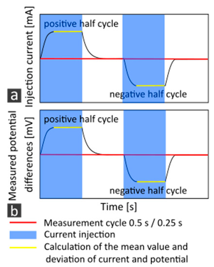
Figure 3.
Sketch of a geoelectric measurement cycle, showing (a) the strength of the injected current and (b) the measured potential differences with time within the time window of two half cycles. The red line describes the full length of either 0.5 or 0.25 s used for the measurements. The blue box highlights the time interval of current injection. The yellow line shows the interval for the calculation of the mean measured value of current and potential, from which the standard deviation is given, defining the measurement noise.
- (a)
- Noise: As it is common for geoelectric instruments, the injected currents and related potential differences are reversed in polarity during one measurement cycle and follow typical rise and decay time functions (Figure 3). The recording unit evaluates the quality/noise level within the time intervals of the plateaus of the step functions and accepts or declines a single apparent resistivity value due to a selectable threshold. Single events, such as water waves, contribute to the noise level and are thus recorded by the acquisition unit. We quantify “noise” as the standard deviation of a single measurement within the time intervals of two half cycles (Figure 3, yellow line) during a measurement cycle of 0.25 or 0.5 s (Figure 3, red line) from their average value corresponding to the measured resistivity value [13].
- (b)
- Smearing effects: In setup T, the continuous movement of the electrode streamer causes a spatial “smearing” of data values along the profile (“inline”) during one cycle. This also affects the standard deviation of the single measurements within the intervals of two half cycles (Figure 3, yellow line) and can therefore not be distinguished from noise. Therefore, we do not consider this effect separately. It results in an increased standard deviation for setup T and is included in the term “noise”.
- (c)
- Streamer deflections: Uncertainties in apparent resistivity are also caused by deflections of the electrode streamer that result from wind and swell, especially during towed prospections. Streamer deflections change the electrode spacing and, therefore, the geometry factor required for computing the apparent resistivity values. To estimate this error type, we assume a relative inline displacement e = 10 cm of each streamer end with respect to their midpoint (Figure 4). Since the length b of the streamer remains constant, this displacement causes a deflected streamer that we assume to be approximated by the shape of a circle segment, such that the streamer midpoint is displaced by a distance, a, orthogonally from the inline direction. In this geometry, the streamer is an arc segment of length b and its ends are connected inline by a secant of length s. The midpoint displacement a can be calculated using the center angle of the arc α and the circle radius r according to:
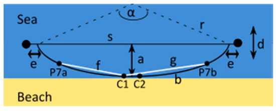 Figure 4. Simplified drawing of measurements carried out parallel to the coastline, causing a deflected streamer, approximated by the height of a small circle segment. α is the center angle of the arc, r is the circle radius, b is the length of the streamer, s is the secant, a is the orthogonal displacement from the midpoint and e is the relative inline displacement. C1 and C2 are the current electrodes, P7a and P7b are the potential electrodes, f is the distance between P7a and C1 respective to P7b and C2 and g is the distance between P7a and C2 respective to P7b and C1.From this, the geometry factor k can be calculated from the symmetrical distance of and (Figure 4) for floating electrodes:and for submerged electrodes using the mirror source technique, depending on the water depth tw:The uncertainty for the apparent resistivity of an electrode pair results from the difference of the geometry factor for the straight and deflected cable and the arithmetic mean value for the repeated measured current and voltage.
 - (d)
- Effective water-level variations: There are two effects, which we combine into an “effective water-level variation”. The first one is swell, which displaces the electrodes in the vertical direction, thus changing their distance to the sea bottom. It depends on the speed, lengths and heights of the water waves. The second effect is the possible variation of bathymetry in the cross-line direction, which affects the measurements through the varying cross-line deflections of the streamer. Quantifying these effects in an exact way would require, besides bathymetry, accurate knowledge of the 3D positions. As this is hardly achievable, we attempt to estimate the order of magnitude of the resulting uncertainties by assuming that they can be modelled by the temporal variation of an “effective water-level”. For this purpose, we compute the apparent resistivity values for a set of two-layer (2L) models. The thickness of the upper layer, identified with the water column of 0.3 Ωm resistivity, is varied between 0.8 and 1.2 m in intervals of 10 cm. At an average water depth of 1 m, the curves correspond to an effective water-level variation of ±10 and ±20 cm. For the bottom layer, resistivity values of 1 and 100 Ωm were chosen. A bottom resistivity of 1 Ωm corresponds to saturated sand or clay, whereas a bottom resistivity of 100 Ωm corresponds to saturated limestone [14]. In order to estimate the measurement uncertainty for the different setups, an effective water-level variation of 5 cm was assumed for setup S, of 10 cm for setup F and of 20 cm for setup T. The uncertainty is defined to be the difference between apparent resistivity of the average water depth and of the maximum water displacement.
- (e)
- Repeatability of profile locations: To complete the considerations on the errors of the three measurement setups (F, S, T), the general positioning uncertainty of the mid streamer point was evaluated in inline and cross-line directions using the data of setup T, which is assumed to have the largest uncertainties in positioning. This was estimated using the deviations of the GNSS (global navigation satellite systems) coordinates from the mean profile track, the possible streamer deflections and the inline “smearing interval length” of data due to the streamer movements during a measurement cycle for setup T. The positioning uncertainty provides effective water-level variations in a sloped seafloor, similar to cable deflections, and thus uncertainties in apparent resistivity. They have been summarized above in point (d). In addition, the positioning uncertainty restricts the prospection of laterally limited objects.
2.2.2. Inversion Reproducibility
We tested the reproducibility of inversion results from eight repeated profiles in Eckernförde Bay for all three setups. The inversions were carried out with the software RES2DInv [17]. We did not provide a priori information with the inversion for setup F and T. However, the specification of water depth and water resistivity was required for setup S. From the inversion results of eight repetition profiles, mean values and standard deviations were determined for each setup. For setup T, an inline data bin size of 1 m was compared to a lower bin size of 30 cm.
2.3. Resolution of Layer Thickness and Resistivity in 1D Media
We investigated the resolution of layer thickness and resistivity for our inverse Schlumberger streamer with different measurement setups based on numerical studies of 1D cases with 2L and 3L/4L models and on field measurement uncertainties. This involved:
- Forward modelling of layered media, to investigate which apparent resistivity values and layer thicknesses can be differentiated due to field measurement inaccuracies in a number of scenarios for setups F, S and T.
- Stochastic inversion of the forward modelled data for setups F and S to investigate how the results of the forward modelling affect equivalent solutions of layer thickness and resistivity during the inversion.
2.3.1. Forward Modelling of Layered Media
In order to understand the characteristics of geoelectric measurement curves in shallow water, we calculated Schlumberger sounding curves comparing shallow-water and onshore settings. To approximate sediment and rock below a water layer, we have defined three possible 2L scenarios (Figure 5a–c). They correspond to shallow water (Figure 5a,b) and to onshore settings (Figure 5c). The shallow water settings are based on the 2L case shown in Figure 1, with a brackish water column of 1 m depth and a second layer of material varying from saturated clay to granite. Specific resistivity values from 1 to 1000 Ωm were chosen in irregular steps. Offshore archaeological features are often sanded in shallow depth underneath the seafloor (see also Figure 1e). Targets such as wrecks or harbor constructions may extend horizontally over several meters, but much less in depth. This motivated us to make an attempt to assess the arrays’ ability to locate this type of target. Therefore, we have defined three 3L cases (Figure 5d–f), again comparing shallow water (Figure 5a,b) and onshore settings (Figure 5c). Here, we included a 1 m thin sea-bottom layer over a half-space thought to represent an archaeological feature. The third layer satisfies the criteria for moistened sand. In the onshore scenario, the 1 m thick water layer was replaced by moistened sand, and the other layer parameters were kept constant. The measurement configurations selected were setup F (Figure 5b) and S (Figure 5c) for shallow water settings. For the onshore settings, electrodes at the surface were used. The formulae for computing theoretical sounding curves were derived for the Schlumberger configuration. However, because of the reciprocity theorem, they also apply to the inverse Schlumberger configuration. They are given in the Appendix A, where floating and submerged electrodes are differentiated.
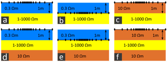
Figure 5.
Subsurface models used for forward calculations in the 2L case for (a) a shallow water environment, setup F, (b) a shallow water environment, setup S and (c) an onshore environment, as well as in the 3L case for (d) a shallow water environment, setup F, (e) a shallow water environment, setup S and (f) an onshore environment.
Based on the sounding curves, we followed further considerations to investigate which specific subsurface resistivity values can be resolved based on the measurement uncertainty of the three measurement setups using forward modelling:
- We calculated the required streamer length for an inverse Schlumberger configuration to differentiate the specific resistivity of the subsurface from a 2L case. We distinguished between a shallow water and an onshore scenario, in which the depth of the first layer is varied.
- We defined a 2L shallow water scenario with a brackish water column of 1 m depth and a subsurface resistivity of 1, respectively 10 Ωm. The streamer used for the field measurements in Section 1 was chosen for the measurement configuration. We inserted a layer of variable thickness and resistivity into the homogeneous half-space of the 2L case at a variable depth, resulting in a 3L or 4L case. We investigated the conditions at which the layer can still be differentiated from the homogeneous half-space.
- 1.
- Required Streamer Length in the 2L Case
We calculated the required streamer length to differentiate between subsurface resistivity values with a tolerance of 100%. First, we calculated the apparent resistivity for specific resistivity values of 1 to 1000 Ωm as a function of the electrode layout of 1 to 1000 m. Then, we calculated the apparent resistivity values for the doubled resistivity values described above for the same electrode layout. For each streamer length, the apparent resistivity values are subtracted from each other. The required length is reached when this difference is more than three times larger than the field measurement uncertainty, depending on the measurement setup.
- 2.
- Resolution of a Layer in the Sea Bottom (3L/4L Case)
To determine the resolution of a layer in the sea bottom, we calculated sounding curves for the 3L/4L case within the following ranges: The specific resistivity of the layer ranges from 1–1000 Ωm and thickness of the layer is 0.1–1.8 m. The depth of the layer is 0–10 m below the 1 m deep sea bottom and the specific resistivity of the half-space is 1 and 10 Ωm. Then, the quotient is calculated from the 3L/4L case with an embedded layer and the 2L case (with a sea bottom resistivity of the half-space). For eight quotients for each measurement curve, the variance with respect to the value 1 is calculated and then a one-sided F-test is done. Thus, 2L and 3L/4L curves can be separated from each other with a probability of 95% if the calculated variance is greater than a multiplied factor (here, 2.1, depending on the degrees of freedom) of the squared measurement accuracy. The measurement accuracy depends on the chosen measurement setup.
2.3.2. Calculation of Equivalent Model Solutions by Stochastic Inversion by Particle Swarm Optimization
After examining sounding curves, we wanted to investigate to what extent measurement uncertainties affect ambiguities of inversion results. We applied stochastic inversion as a statistical approach to quantify equivalent model solutions within a defined parameter space. For this purpose, we chose the particle swarm optimization method, after Reference [18]. It was applied to minimize the misfit between modelled sounding curves and our exemplary curve, measured at Eckernförde bay, and to explore the space of suitable models at the same time. Furthermore, interdependencies of the subsurface parameters can be quantified. Here, so-called particles (different models, ) of a “swarm” (a certain number of models) are randomly chosen and then move through the parameter space searching for minimum misfit solutions within a value range. The moving corresponds to adding a movement vector, to each particle of an iteration step, t. The new particle (comprising the subsurface parameters (resistivity, ρi, and thickness, hi, of a layer, i)) of iteration t + 1 is then
The search direction of each particle consists of a weighted sum of the initial search direction or search direction of the last iteration, the direction to the individual best solutions of one particle, mi, as well as the direction to the global optimum solution of the whole swarm, mg.
where ω and c1, c2 are weighting factor, and and are uniformly distributed random number vectors out of (0,1), that randomize the search direction. The basic particle swarm optimization used here is extended by an option that resets the whole swarm, if stagnation occurs, and a local search algorithm starting at mg after each swarm movement, following the approach of Reference [19].
Based on the huge amount of forward calculations done for a particle swarm optimization, an estimate of the probability density function of the model parameters can be determined, enabling to calculate an expected model solution as well as the variance of the model parameters (main diagonal of the covariance matrix). Furthermore, possible trade-offs between model parameters can be investigated (other entries of the covariance matrix) (e.g., Reference [19]). To apply the method for a geoelectric 2L case, using both setups F and S, we first created 300 random model solutions each consisting of three parameters: the specific resistivity of the first (ρ1) and second layer (ρ2) and the depth of the first layer (h1). The parameter range or search space is defined from the 2L model solution of an exemplary sounding curve recorded from the Eckernförde test profile with setup F using the software IX1D by Interpex [20]. The parameter values are 0.3 ± 0.29 Ωm and 80 ± 79 Ωm for the resistivity values of the first and second layers, and 0.9 ± 0.5 m for the depth of the first layer. The method was also applied for a 3L case for setup F and S, for which again 300 random model solutions were created consisting of five parameters: the specific resistivity of the first (ρ1), second (ρ2) and third layer (ρ3), as well as the first and second layer thickness (h1 and h2). Here, the parameter range corresponds to that of the 2L case, extended by a third layer. It is defined by 0.3 ± 0.29 Ωm, 80 ± 79 Ωm and 10 ± 9 Ωm for the resistivity values of the first, second and third layers respectively, and 0.9 ± 0.8 m for the layer thicknesses. To enable the swarm to leave local minima, the swarm is randomly redistributed after 25 iterations if the global misfit change is <6 × 10⁻⁵. In total, the misfit values of 1800 models of the first six iterations are used to calculate the probability density function. The variance of each model parameter is defined as the square of the covariance matrix. A normalized correlation matrix was calculated from the covariance matrix to identify possible correlations of the subsurface parameters.
2.4. Resolution of Layer Thickness and Resistivity in 1D Media
To investigate the spatial resolution of 2D applications below the sea bottom, we applied two approaches:
- Calculate sensitivity kernels for setup F, S under consideration of the water column.
- Perform checkerboard tests for setup F, S.
2.4.1. Sensitivity Kernels
The sensitivity kernel describes the effect of a single point-shaped resistivity anomaly on the potential or measured potential difference for a given electrode geometry. It depends on the relative positions of the anomalies and electrodes, the resistivity distribution of the background and the anomaly contrast to this background. The authors of Reference [17] considered the potential of an electric monopole, at which a unit-current (1 A) is fed into a homogeneous half-space. They showed that the change of the potential V at an observer position caused by an anomalous resistivity volume Φ can be calculated by:
where ρ is the background resistivity, δρ is the resistivity difference of the anomalous volume with respect to the background and V’ is the “adjoint potential” of an electric monopole placed at the observer position. Considering a 2D medium with electrode and anomaly placement in the x-z-plane, the sensitivity kernel for the monopole potential is:
The sensitivity kernel for the Schlumberger array is then the summation of the four combinations between current electrodes C1 and C2 and the exemplary chosen potential electrodes P1a and P1b:
For electrodes at the surface, the potential V can be calculated by using the half-space formulas (see Appendix B). For submerged electrodes, the full-space formulas for the potential V (see Appendix B) and the mirror source technique have to be used:
Sensitivity kernels were calculated for a water layer of 1 m depth and 0.3 Ωm over a half-space media of 10 Ωm by Formula (8).
2.4.2. Checkerboard Tests
After calculating the 2D sensitivity kernels for our inverse Schlumberger streamer, we used synthetic data to verify the results. In Reference [8], numerous investigations on isolated objects in a homogeneous half-space have already been done. We are particularly interested in the spatial resolution of multiple small-scaled objects, that are aligned in both lateral and vertical direction, and in the resulting limitations of the different measurement setups. For this purpose, a checkerboard test is useful, where numerous objects are located with vertical and lateral distance. We distinguished between three synthetic subsurface models of 30 m length and 4 m depth, approximating both onshore and shallow water scenarios. The checkerboard pattern consists of 1 × 1 m large bodies with alternating resistivity values of 1 and 10 Ωm in the sub-bottom. These values correspond to typical contrasts in the subsurface, such as wet sand to weathered rock. They are well-resolvable using our inverse Schlumberger streamer in the 1D case, so that the focus can be set on the 2D resolution. An additional water column of 1 m depth and 0.3 Ωm was implemented for the shallow water case. Again, setups F and S were compared using a 20 m Schlumberger array. As the forward modelling was performed with the software RES2DMOD [21], we used an equal electrode distance of 1 m. Nevertheless, this is comparable to our array due to the same streamer length and a similar minimum electrode spacing. The horizontal and vertical cell spacing was 0.25 and 0.5 m. Noise of 1% and 2% was added to the data for the measurement setup S and F. The inversion was done with the software RES2DInv [17]. In cases where the checkerboard test could not provide a spatial separation between the objects, the object arrangement was varied (i.e., using no vertically arranged objects, an increased object size or a larger lateral object spacing) to investigate the possibilities of each measurement setup.
3. Results
3.1. Repeated Field Measurements
In the following sections, results of the repeated field measurements are presented. First, the measurement uncertainties are shown before focusing on the reproducibility of 2D inversion results.
3.1.1. Measurement Uncertainty
The measurement errors from the 2D repeated measurement profile for setups S, F and T are shown in Figure 6 and in Table 2 and Table 3. Figure 6a–c show pseudo sections of arithmetically averaged apparent resistivity values from repeated measurements for eight pairs of electrodes (y-axis) and 40 positions along the profile (x-axis). The apparent resistivity values increase with larger electrode spacing, indicating the transition from the water column to the sea bottom. The pseudo sections of all three setups are compatible, showing apparent resistivity values of 0.5 to 4 Ωm. The apparent resistivity values of setup S are slightly higher due to the proximity of the electrodes to the sea floor. The relative (1σ) standard deviations occurring for each electrode layout and profile position are displayed in Figure 6d–f. The maximum uncertainties are of the order of 1% for the static measurements and a few % for the moving system. In particular, we found the stationary setups S and F showing average uncertainties of < 0.8% and < 1.5% respectively, whereas the moving setup T showed uncertainties < 5%. The values are given numerically in Table 2. The uncertainties increase with depth for stationary measurements. Noticeable are disturbances affecting all electrode pairs at particular profile positions. Setup T shows the largest uncertainties for the fourth to sixth electrode pair in the middle of the measurement profile. Table 2 also summarizes further investigations of the setup T regarding a possible impact of various measurement cycle lengths of 0.25 and 0.5 s (see Figure 3), of the chosen inline bin sizes of 30 cm and 1 m respectively, and of the towing direction with or against the wind on the measurement uncertainties. None of the aspects have a significant influence on the occurring uncertainties. However, a short measurement cycle of 0.25 s for towed measurements is rather obstructive, whereas setup F is not dependent on the measurement cycle (Table 3).
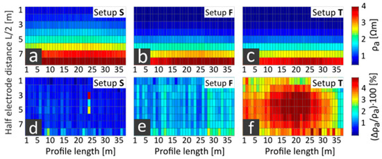
Figure 6.
(a–c) Mean values and (d–f) relative standard deviations from repeated measurements for eight electrode pairs (y-axis) along the profile (x-axis). Left column: setup S (submerged), center column: setup F (floating), right column: setup T (towed).
Table 2.
Summary of relative standard deviations for different measurement setups arithmetically averaged from 40 measurement positions for the most affected electrode layout (L/2 (m), see Table 1). Additional aspects such as the bin size, the towing direction depending on the wind and the measurement cycle length are listed.
Table 3.
Relative standard deviations (1σ) for various measurement cycles of setup F. The values are determined from a single measurement position for an electrode layout of L/2 = 10 m.
In the next step, we investigated possible uncertainty sources. Table 4 summarizes three assumed error components for the exemplary electrode pair P7a–P7b, with L/2 = 7 m for all measurement setups. The noise was derived from the field measurements, whereas deviations due to streamer deflections and water-lever variations were theoretically estimated. With relative uncertainties of approximately 1%, 2% and 5% for setup S, F and T, the noise is equal to the average measurement accuracy for the electrode pair P7a–P7b. Thus, for larger electrode layouts, we assume that other sources of error will only contribute to the maximum recorded uncertainties. For the shortest layouts (L/2 = 0.75 m), as an example, the noise for setup F is 0.3%, so that other sources of error are more evident here. Figure 7 compares measurement uncertainties of setup F from field data shown in Figure 6 and Table 2, with theoretical uncertainty calculations based on estimations made in Section 2.2.1, including water-level variations and streamer deflections. The effective water-level variations are shown by colored vertical electrode sounding (VES) curves and appear to affect the apparent resistivity values more than streamer deflections (Figure 7, red error bar, relative errors of 2%). The influence of water-level variations on the apparent resistivity increases with increasing subsurface layer resistivity (compare Figure 7a, computed for 1 Ωm, and Figure 7b for 100 Ωm). Measurement uncertainties obtained from the repeated profiling with setup T (Figure 7, black error bar) are within the range of effective water-level variations of 10 cm for a subsurface resistivity of 1 Ωm, and uncertainties of stationary measurements (Figure 7, blue error bar) are even smaller. Compared to the calculated water-level variations on a subsurface resistivity of 100 Ωm, the measured uncertainties are of little weight. Thus, we assume that water-level changes occur locally and do not change the total water column, as considered in the calculation. On the contrary, for resistivity values ~ 1 Ωm, the height of the water column might be incorrectly determined by ±10 cm due to measurement uncertainties. Since Table 4 includes the maximum possible impact of water-level variations and cable deflections, the estimated measurement uncertainties are significantly higher than the observed uncertainties. As observed with the repeated field measurements, setup T shows the largest uncertainties followed by setup F and setup S.
Table 4.
Measurement errors resulting from noise, streamer deflections and water-level variations are estimated for an electrode of L/2 = 7 m and compared among the measurement setups.
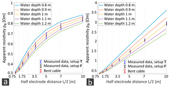
Figure 7.
Sounding curves of a 2L case for various water depths (colored curves) and a first layer resistivity of 0.3 Ωm and a second layer resistivity of (a) 1 Ωm and (b) 100 Ωm. Errors of setup T (blue error bars), setup F (red error bars) and streamer deflections (black error bars) from Eckernförde Bay repetition measurements are added.
To conclude the section, the repeatability of profile locations of setup T was evaluated in inline and cross-line directions. The maximum inline position deviation of ±50 cm results from “smearing effects” of ±30 cm and from errors due to streamer deflections of ±10 cm. A histogram of cross-line GNSS coordinate deviations, d, from the mean profile track (see also Figure 3) is shown in Figure 8. The cross-line profile track error of 50 cm was defined as twice the standard deviation and complemented by cross-line streamer deflection deviations of ±1 m for the fourth electrode pair of L/2 = 2.50 m (see also Figure 4). This results in a maximum error of ±1.50 m within the cross-line direction. Within this range, we expect measurement errors due to water-level variations or smearing of the apparent resistivity caused by a possible 3D distortion of target locations.
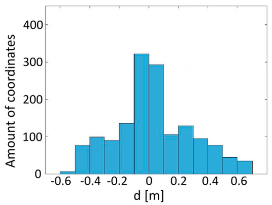
Figure 8.
Histogram of GNSS (global navigation satellite systems) coordinate deviations, d, of all towed profiles from the average measurement profile calculated from a regression curve of the coordinates.
3.1.2. Inversion Reproducibility
After investigating the repeatability of measurement values of a profile and possible sources of uncertainties, the reproducibility of 2D inversions of the same profile is considered. In Figure 9a–c, the arithmetical average of eight individual inversion results from the repetition profiles are compared for setup S (Figure 9a), setup F (Figure 9b) and setup T (Figure 9c). In general, the average inversion results of setup S, F and T are similar with regard to the water resistivity, water depth and lateral resistivity distribution in the sub-bottom, showing a lateral trend from low resistivity values of 50 Ωm at the left profile side to resistivity values of > 150 Ωm at the right profile side. The water column corresponds to the on-site measurements regarding depth and resistivity. For setup S, slightly higher values of the water and sub-bottom resistivity were observed. In Figure 9d–f, the relative standard deviations of the inversion results are compared for the three setups. The water column is well reproduced with all setups, showing deviations < 5%. The reproducibility of subsurface resistivity values is almost comparable to those of the water column with deviations < 10% for setup F. In comparison, setup T shows increased relative standard deviations of >10% in the subsurface. Setup S shows local deviations of >20%.
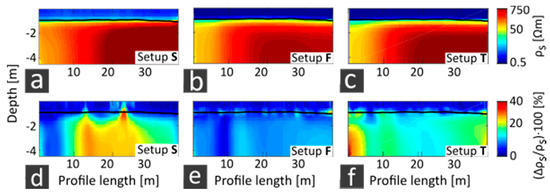
Figure 9.
Comparative plotting of (a–c) arithmetical average values and (d–f) relative standard deviations of eight two-dimensional (2D) inversion results calculated from repetition profiles of Eckernförde Bay with the software RES2DInv. (a,d) Setup S (submerged), (b,e) setup F (floating) and (c,f) setup T (towed).
3.2. Resolution of Layer Thickness and Resistivity in 1D Media
3.2.1. Forward Modelling of Layered Media
We investigated the spatial resolution of our Schlumberger array (largest half electrode distance, L/2 = 10 m, see Table 1) by comparing the theoretical sounding curves of possible onshore and shallow water environments for different layering of 2L and 3L cases (Figure 10). We then focused on a 2L case, where we basically investigated the influence of varying sea bottom resistivity and water depths for the three setups on the required streamer length. Then, we turned to a 3L/4L case were we investigated the resolution ability of the setups with respect to a layer in a homogenous sea bottom thought to represent an archaeological feature.
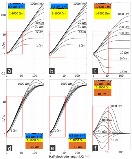
Figure 10.
Schlumberger sounding curves for a 2L case (top row) and a 3L case (bottom row). 2L case: fixed top layer of 1 m depth and 0.3 Ωm for (a) setup F, (b) setup S and 10 Ωm for (c) an onshore scenario. The resistivity of the second layer varies from 1–1000 Ωm. 3L case: fixed top layer of 1 m depth and resistivity values of 0.3 Ωm for (d) setup F, (e) setup S in a shallow water environment and 10 Ωm for (f) an onshore scenario. Resistivity values of the second layer (1 m depth) vary from 1 to 1000 Ωm, the third layer is fixed with 10 Ωm. Red box: array length used within the field measurements.
Sounding Curves for the 2L and 3L Case
As shown in Figure 10, for the shallow water 2L scenarios, the variation span of apparent resistivity due to sea bottom resistivity is reduced by a factor of 100 compared to the variation of “true” sea bottom resistivity within the observation window of the streamer system (red boxes in Figure 9). In a first assumption of the measurement uncertainties, all setups are able to distinguish between sea bottom resistivity values in the range of 1 to 10 Ωm. However, sea bottom resistivity values of > 10 Ωm appear to be almost undistinguishable. The main difference between the setups S and F is visible for array lengths < 5 m and for subsurface resistivity values < 5 Ωm. In this case, setup S shows apparent resistivity values of a full-space environment. This is different for the onshore case (Figure 10c), where the higher resistivity of the surface layer enables a differentiation of bottom-layer resistivity values according to first estimates in the range of 1 to 200 Ωm, given the same uncertainties and spread lengths as in the shallow water case. Indeed, the ratio of the resistivity of the top layer to the maximum resolvable resistivity of the bottom layer is in both cases about the same (about 0.5%) and approximately equal to the measurement uncertainty. In the 3L case, for specific resistivity values of the middle layer of 1–1000 Ωm, the resulting range of apparent resistivity values is 70 times higher in the onshore scenario (4–70 Ωm, Figure 10c) than in the shallow water scenario (2.1–3 Ωm, Figure 10a, b) for our streamer length. The maxima of the 3L sounding curves are far out of the streamer length for the shallow water scenario. Therefore, 2L and 3L sounding curves are quite similar, depending on the subsurface. This issue is discussed in detail in the section below. The difference of setup S (Figure 10e) and setup F (Figure 10d) in the shallow water scenario is again visible for small array lengths < 2 m and low subsurface resistivity values < 5 Ωm.
Required Streamer Length in the 2L Case
Figure 11 shows the required streamer length to resolve the specific resistivity of the subsurface in a shallow water 2L case with a tolerance of 100% considering the measurement uncertainty. Variations of the water column from 0.2 to 2 m and the differences of the setups S, F and T were evaluated. There is a significant difference between the shallow water scenario (Figure 11a–c) and the onshore scenario (Figure 11d). In the onshore scenario, specific resistivity values > 100 Ωm with a surface layer thickness up to 2 m can be resolved with our electrode array of 20 m length. In the shallow water scenario, a specific resistivity of about 10 Ωm can be well resolved in water depths depending on the measurement setup (0.4–2 m). The required streamer length increases with increasing resistivity contrast from the bottom to the top layer. In the onshore scenario, this increase can be observed from a specific resistivity of 10 Ωm. In contrast, due to the top layer of 10 Ωm, for specific resistivity values of 1–10 Ωm, there is a little decrease in the required streamer length. Furthermore, for the shallow water scenarios, setup S can resolve a specific resistivity that is seven times lower than setup T for an equal streamer length and water depth. A duplication of the water depth requires twice the streamer length in order to resolve the same specific resistivity values.
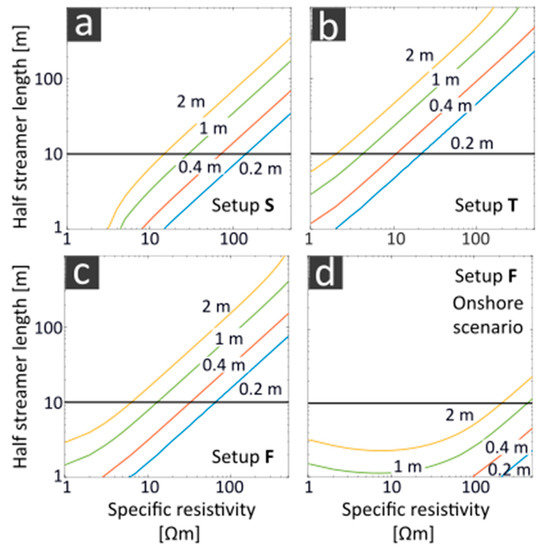
Figure 11.
Required streamer length (y-axis) to resolve the specific resistivity of the homogeneous half space of a 2L case (x-axis) with a tolerance of 100%. We differentiate between (a–c) a shallow water and (d) an onshore scenario and the measurement setups (a) S (submerged), (b) T (towed) and (c,d) F (floating). We used water depths from 0.2 to 2 m.
Resolution of a Layer in the Sea Bottom (3L/4L Case)
Figure 12 shows the required parameters to differentiate an embedded layer from the surrounding sea bottom. A brackish water column of 1 m was used to calculate the maximum depth in which variable layer resistivity values and thicknesses can be resolved due to the measurement uncertainties. For all measurement setups and layer resistivity values, the relation between the layer thickness and its maximum resolvable depth can be described by limited growth functions. For setup S and F, the maximum layer depth is not reached at any investigated layer resistivity and thickness in a sea bottom of 1 Ωm. For setup T, this applies to resistivity values larger than 200 Ωm. The maximum detection threshold of approximately 8 m depth is reached from a layer thickness of 0.5 m (Figure 12b). Setup S shows the lowest measurement uncertainty. Here, resistivity values > 20 Ωm can be resolved for layer thicknesses > 0.5 m in more than 10 m depth below the sea bottom (Figure 12a). For setup F, this applies to resistivity values > 100 Ωm (Figure 12c). For a sea bottom of 10 Ωm, the limited growth curves for specific resistivity values of 50–100 Ωm and 2–5 Ωm are in the same range (Figure 12d). Here, comparable layer thicknesses and layer depths can be resolved. From all investigations, the lowest depth resolution is reached here, which is due to the lower contrast of the layer resistivity values to the sea floor.
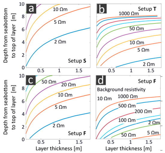
Figure 12.
Plot of the maximum depth to which a layer of variable thickness and resistivity can be differentiated from the surrounding sea bottom. The depth is defined as the distance between the sea floor for a brackish water column of 1 m to the upper edge of the layer. The sea bottom shows resistivity values of (a–c) 1 Ωm and (d) 10 Ωm. The measurement uncertainties of setup (a) S (submerged), (c,d) F (floating) and (b) T (towed) are compared.
3.2.2. Calculation of Equivalent Model Solutions by Stochastic Inversion Using Particle Swarm Optimization
In the last Section, we have shown that in shallow water environments, the sounding curves of an inverse Schlumberger configuration for both 2L and 3L/4L cases with varying specific resistivity values in the sea bottom are close to each other. Due to measurement uncertainties for each setup, specific resistivity values in the subsurface cannot be properly differentiated. Consequently, ambiguities will occur during the inversion. In this chapter, we focus on the question of how significant these ambiguities are. For this purpose, we analyzed two exemplary 2L and 3L models. The 2L model is based on the 1D inversion result of a measurement curve taken from the profile of Eckernförde Bay. There is a water layer of 0.3 Ωm and 0.9 m depth, as well as a sediment resistivity of 80 Ωm. For the 3L case, we have assumed a second layer of 90 cm and 80 Ωm, as well as a half-space resistivity of 10 Ωm. The measurement uncertainties of the setups S and T were used to weight the inversion solutions.
Resolution of Sediments Below the Water Column (2L Case)
In the stochastic inversion, six iteration steps were stored for each model. From the pool of all solutions, those with a relative deviation of <14% to the reference model were selected to be shown in Figure 13a for a better visualization of the inversion ambiguities for setup F. The particular least-square misfit of the model solutions to the true model (black line) is color-coded, and the maximum relative misfit of 14% was normalized to 1. There are slight ambiguities in ρ1 and h1 and a wider range of ambiguities in ρ2. These observations can also be quantified by statistical analysis. Table 5 summarizes the expected model (see also Figure 13a, white dashed line) and its variance of the subsurface parameters. It becomes apparent that the method is sensitive to the resolution of the water column. In the sea bottom, on the other hand, limitations of the method have to be accepted if the array length is not increased. Furthermore, the correlations of the subsurface parameters can be derived from the statistical analysis. Figure 13b shows the normalized correlation matrix of the subsurface parameters of the 2L case for setup F. The main diagonal of the pattern shows the correlation of the parameters with themselves (variances). The remaining pattern describes the correlation coefficients between the subsurface parameters. A large correlation coefficient causes a high dependence of a subsurface parameter on another in the inversion result. In the 2L case, the parameters ρ1 and h1 show this dependence. The correlations offer chances to improve inversion ambiguities by providing information on a parameter (e.g., the water depth) during the inversion. The unambiguous solution of the other parameter (e.g., the water resistivity) is derived from this. However, it also includes risks in the case that erroneous information is given for a parameter in the inversion. An erroneous specification of the water depth results in an incorrect water resistivity. If incorrect a priori information on both water resistivity and depth is given, this will have an impact on the sea bottom resistivity. In a 2L case, setup S shows the same results as setup F with regard to both ambiguities and correlation coefficients.
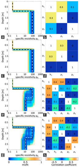
Figure 13.
Left column: Model results from the stochastic inversion, color-coded by their misfit values and normalized to the relative misfit of 14%. The black line represents the true model, and the white dashed line represents the expected model. Right column: normalized correlation matrix of the subsurface parameters. (a,b) Case 2L and setup F, (c,d) case 2L and setup S, (e,f) case 3L and setup F as well as (g,h) case 3L and setup S are distinguished.
Table 5.
Expected model and variance calculated from all models saved during the stochastic inversion using six iteration steps. The subsurface parameters’ layer thickness hi and resistivity ρi are distinguished for the 2L and 3L case as well as for setup F and setup S.
Resolution of a Layer in the Sea Bottom (3L Case)
The analysis of inversion ambiguities in the 2L case was also applied to the 3L case for setup S and F (Figure 13c,d). The results for the 2L and 3L case show parallels and again, the setups hardly differ. The three additional subsurface parameters enlarge the range of possible inversion solutions, and due to measurement uncertainties, the equivalence principle applies. The water column is also best reproducible with < 15% variance. For all sea bottom parameters, there are the same restrictions as in the 2L case, with > 20% variance. In addition to ρ1 and h1, the parameters h1 and h2, as well as ρ2 and ρ3, also correlate with each other. The correlations provide additional options to limit inversion ambiguities. The resistivity of the second layer can also be restricted in case the resistivity of the homogeneous half-space in the area surrounding the prospected objects is known. In contrast to the 2L case, the water depth directly influences the thickness of the second layer. Consequently, erroneous a priori information on the water depth has an increased impact on the sea bottom.
3.3. Spatial Resolution in 2D Media
In the previous sections, we have investigated the resolution of layer thickness and resistivity for 1D sounding curves by forward modelling and stochastic inversion. The next step is to focus on the resolution of objects with defined lateral dimensions in 2D measurements for the three measurement setups. Therefore, the sensitivity kernels of the streamer configuration were calculated and inversion results from synthetic data approximating numerous objects were evaluated.
3.3.1. Sensitivity Kernels
Sensitivity kernels are dependent on the electrode configuration and show a sequence of positive and negative sensitivity areas, from which conclusions can be drawn about the spatial resolution of subsurface targets. The 2D sensitivity kernels of our inverse Schlumberger array in a water column of 1 m depth and 0.3 Ωm above a sub-bottom resistivity of 10 Ωm are compared for setup F (Figure 14a) and setup S (Figure 14b). Both setups show a typical Schlumberger sensitivity pattern with its sequence of positive and negative sensitivity values in lateral direction and the change of positive sensitivity values in vertical direction, that describes the good compromise of vertical and lateral resolution of the method. However, for setup F, the lateral highly sensitive area of the array (see black frames in Figure 12) is found within the water column. At the seafloor, the sensitivity values remain slightly positive for half array lengths < L/2 = 3.5 m. It is only half array lengths > L/2 = 5 m that show low negative sensitivity values in the sea bottom. For setup S, the sensitivity kernels adapt to a full-space environment with a negligible influence from the sea surface boundary. This is noticeable by the pattern around the potential electrodes being minimally orientated towards the sea surface. The sensitivity values of setup S are also in accordance with those of setup F. However, the sequence of positive and negative sensitivity values can be observed in the water column as well as in the seafloor. In addition, at the seafloor, the width of the positive sensitivity cone in the middle of the array is different for the two setups: It is 2 m for setup F and 0.5 m for setup S. However, the maximum depth of the positive sensitivity cone in the middle of the streamer for a half array length of L/2 = 10 m differs only slightly for the two setups. It is about 4 m from the sea surface and provides a first estimation of the depth penetration of the array. The alternating positive and negative sensitivity areas in the sea bottom for setup S is essential for a sufficient resolution of objects, including their specific resistivity and dimensions. Thus, setup S is superior to setup F, especially in the resolution of small-scale objects or the differentiation of numerous laterally separated objects. The positive sensitivity area of setup F in the sea bottom ensures that objects of a certain size can be resolved. However, in case of small object dimensions and large resistivity contrast from object to the surrounding seafloor, blurring has to be expected. The smallest width of objects that can be resolved by setup S and F is estimated to be about 0.5 and 2 m from the lateral extent of the positive sensitivity cones at the seafloor. Thus, with a brackish water column of 1 m, the difference in the lateral resolution of objects below the seafloor is a factor of four among the setups.
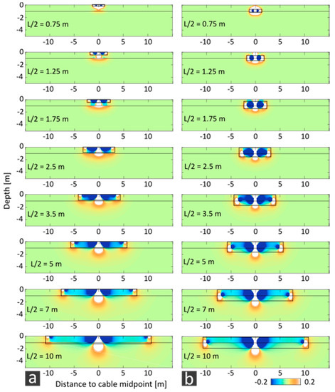
Figure 14.
Comparison of sensitivity kernels from the inverse Schlumberger array used for repetition measurements in Eckernförde Bay, Germany, consisting of eight electrode pairs (Table 1). (a) setup F and (b) setup S are compared, and the lateral highly sensitive area is framed in black.
3.3.2. Checkerboard Tests
After evaluating the sensitivity of the array, we investigated the spatial resolution of multiple objects laterally and vertically arranged in detail using synthetic data. Figure 15 combines the results of the checkerboard tests for an onshore environment (Figure 15a) and for a shallow water environment for setup S (Figure 15b) and setup F (Figure 15c,d). Looking at Figure 15a in detail, the top row of the checkerboard pattern is resolved properly and the subsurface resistivity values of 1 and 10 Ωm are reproduced correctly, whereas the second row’s pattern is blurred and a half-space resistivity value of 3 Ωm is reached. Thus, objects underlying other structures at the surface are hidden, as the second row of the checkerboard pattern can be resolved when the first row is removed. The checkerboard tests approximating a shallow water environment show different results. For setup S, the top row of the checkerboard pattern can still be resolved, although the objects become slightly blurred due to the water column. Additionally, the resistivity values are reduced compared to the original pattern. The inversion results show resistivity values of 0.5 and 5 Ωm above a half-space resistivity of 1 Ωm. Setup F cannot reproduce the checkerboard pattern but shows a horizontally blurred stripe of increased resistivity of 3 Ωm, which indicates the pattern of the first row. Below that, the resistivity values decrease. Based on the results, we modified the checkerboard pattern for this setup and found that vertically arranged objects generally have a significant negative effect on the results. In this case, a minimum object size of 2 × 2 m and a lateral distance of more than 2 m is required for the separation of objects. Figure 15d shows an exemplary object of this size with a lateral separation of 4 m. To resolve numerous objects in the sea bottom, an increased lateral distance between them is required.
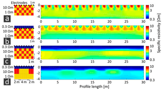
Figure 15.
Left column: Synthetic checkerboard pattern of 1 × 1 m size with subsurface resistivity values of 1 and 10 Ωm, an additional water column of 1 m depth and 0.3 Ωm resistivity for shallow water measurements. For (d), one row of 2 × 2 m pattern size and a lateral distance of 4 m was chosen. Right column: 2D inversions of synthetic checkerboard data. (a) Onshore electrode setup, (b) setup S, (c,d) setup F.
4. Discussion
Based on the results, we discuss the applicability of our inverse Schlumberger streamer with regard to measurement uncertainty, spatial resolution, depth penetration and inversion ambiguity. We also discuss the most suitable measurement setup.
4.1. Repeated Field Measurements
Discussing the measurement uncertainty of different setups, setup S shows the highest reproducibility due to its fixed electrode positions on the seafloor, from which they are largely independent of sea surface waves. For setup F, wind, swell and short periodical waves are of greater importance. Setup T is affected by streamer deflections (Figure 4) and possible resulting water-level variations, which cannot be avoided during the continuous walk along the profile. Furthermore, inline “smearing” effects that occur from a towed streamer movement during a measurement cycle result in higher errors of < 5% (1σ) compared to the other setups. A similar measurement error of 3.5% (1σ) was observed in Reference [12] for a modified Schlumberger streamer, which also had a length of 20 m. Setup S and F show the highest relative errors for large electrode layouts. This is because the electrodes resolving the heterogeneous sea bottom cause larger errors than the electrodes resolving small resistivity variations of the water column. Additionally, the measured potential decreases with increasing array length, amplifying noise. However, stationary repeated measurements also show deviations equally affecting all electrode pairs at one profile position. This can be explained by waves from passing ships that occur spaciously along the surf zone. A surprising feature is that for setup T, the largest measurement errors were recorded for the middle electrode lengths, which is due to the measurement procedure parallel to the coastline (Figure 4). Two persons keep the measurement streamer in track at both ends, whereas the middle of the streamer is hardly manageable and deflects towards the beach, affecting the middle electrode pairs imaging the transition from water column to the sea bottom. As the sea floor slopes down 8.5° towards the sea, the water depth changes, about 15 cm/m perpendicular to the beach, which results in the largest uncertainties for the middle electrode pairs. The high measurement uncertainties in the middle of the profile are because, at the profile beginnings in forward and backward directions, the streamer was still held straight, which reduces the uncertainties. The application of shorter measurement cycles of 0.25 s instead of 0.5 s for a tighter data coverage with setup T is not appropriate—the resolution limits of the method cannot be improved any more. We can improve the data quality when avoiding streamer deflections and measurements affected by long-period waves in the surf zone. Figure 7 and theoretical error estimations for the electrode pair L/2 = 7 m in Table 4 confirm that measurement uncertainties can hardly be estimated—our approaches provided overestimations of uncertainty sources. This is due to sea-level changes, e.g., long-periodical waves, which occur spatially and do not affect the entire sea surface, as expected for the theoretical estimations. Possible streamer deflections change permanently along the profile, and thus, errors are also smaller. Furthermore, uncertainty sources affect each other. A deflected cable causes water-level variations at the same time, which in turn influences the noise level. In summary, the measurement uncertainties cannot be corrected. Therefore, it is important to pay attention to a tidy measurement procedure and calm water conditions.
4.2. Spatial Resolution
An inverse Schlumberger streamer applied in shallow water environments shows limitations in the resolution of layers, respectively object dimensions, and resistivity due to the water column. The evaluation of sounding curves of a 2L case shows that only for a specific resistivity up to 1 Ωm does the apparent resistivity coincide with the specific resistivity of the second layer within our streamer length. Resistivity values up to 10 Ωm can still be differentiated. Similar restrictions are also known for other geoelectrical configurations from the studies in References [9] and [10], investigating VES curves for Wenner α and Dipole–Dipole configurations. Both studies use a water resistivity of 1 Ωm and a maximum sea bottom resistivity of 10 Ωm; nevertheless, the limitation of the “conventional” measurement configurations are already apparent in this case. The foremost improvement would be to increase the streamer length and therefore the electrode layout. With regard to the measurement streamer manageability and increased measurement and position uncertainties for large array lengths prospecting a big subsurface volume, this idea is not practical. Furthermore, coast-parallel measurements become more challenging with a long streamer. A study to overcome the limitations is presented in Reference [11]. However, the approach is suitable for water depths of several meters and sufficient space across profile directions. Thus, “classical” measurement configurations should be chosen according to their sensitivity with regard to the respective issue. The authors of Reference [8] suggest the Pole–Dipole and Schlumberger configuration in the prospection of archaeological objects. The authors of Reference [9] found a high sensitivity of the Dipole–Dipole configuration for thin layers below the sea floor.
Numerous factors can improve the resolution of each measurement configuration, such as the measurement setup, and thus the measurement uncertainties, as well as a low water column and a low resistivity in the sea bottom. As an example, in a 3L case, with setup S, it is possible to differentiate between layer resistivity values that are approximately 5 times larger than for setup F, for the same depth and thickness of the layer. A duplication of the water layer allows, under otherwise equal conditions, to resolve resistivity values in the second layer of a 2L case decreased by the factor 2. The authors of Reference [8] also investigated the influence of the water depth. For instance, a water column of 1 or 2 m makes a difference as to whether an isolated object of 5 × 2 m in size can be resolved at a depth of 3 m or not using a 48 m long Pole–Dipole streamer. The resolution of layers in the sea bottom is more affected by the specific resistivity of the half-space than by measurement uncertainties. A specific resistivity of 1 or 10 Ωm of the half-space defines the resolution of a layer of 50 Ωm and 0.5 m thickness in depths > 10 m or <4 m below the sea floor. Previous knowledge on the subsurface material is therefore useful for the success of measurements.
In addition to the measurement uncertainty, the sensitivity of measurement setups is important for 2D measurements of lateral-limited objects. Thus, the lateral and vertical sensitivity of setup S and F in the sea bottom point out their advantages and disadvantages. These differences of the measurement setups are more important for numerous objects than for isolated objects. The authors of Reference [8] compare synthetic data representing meter-scale, isolated targets for submerged and floating electrodes of different measurement configurations. Their investigations show that submerged and floating electrodes both show good results for a varying target size and target depth for water depths of 1 m. The inversion results show that for submerged electrodes, the targets are located in greater depths than for floating electrodes. Floating electrodes show larger resistivity contrasts for a Schlumberger configuration than submerged electrodes. However, for complicated structures in the subsurface, they recommend using submerged electrodes. This suggestion can be confirmed from our investigations. With numerous objects laterally or vertically arranged, setup S provides a significant advantage. This also affects the prospection of objects in an unknown, heterogeneous sea bottom, with possible natural rock deposits. Setup F often blurs or does not resolve these structures. Due to the water column, the specific resistivity values of the inversion results do not correspond to the material of the objects for both setups.
4.3. Depth of Penetration
The depth of penetration of our inverse Schlumberger array cannot be generalized, but depends on many factors: Measurement uncertainty, object or layer dimensions, depth and resistivity, as well as the resistivity of the surrounding material. In this study, we followed two approaches that provide information about the depth penetration in a brackish water column of 1 m. We calculated sensitivity kernels of our array for floating and submerged electrodes. They define the change in apparent resistivity when the specific resistivity of a small volume in the subsurface is modified. Based on the calculations, our array is sensitive for both submerged and floating electrodes down to a depth of about 4 m. This can provide a first approximation for the planning of measurements. However, layers can also be resolved in larger depths. In our second approach, we have investigated the change in apparent resistivity due to an embedded layer in a homogeneous half-space, below the sea floor. In general, for lower resistivity values of the half-space, a layer can be resolved in greater depth. The approach also shows that there is a maximum depth of penetration regardless of layer thickness and resistivity. The maximum depth penetration was reached with setup T for layer thicknesses of 0.5 m and specific resistivity values of 1000 Ωm in depths of approximately 9 m for a half-space resistivity of 1 Ωm. In our investigations, the maximum depth penetration for setups S and F was not reached here. For a half-space resistivity of 10 Ωm, a layer resistivity of 1000 Ωm and thickness of 2 m, the penetration limit for setup F is approximately 8 m. It is essential that the sea bottom above the embedded layer is homogeneous. Our investigations using checkerboard tests show that for numerous objects laterally positioned, underlying layers are blurred. This effect should also be considered when debris has to be expected on the sea floor, for example.
4.4. Inversion Ambiguity
The results of the stochastic inversion show that the strengths of marine geoelectric measurements are the prospection of the water column. Therefore, the method is suitable to investigate stratifications in the water column (caused by salinity and temperature). Objects in the water column can also be an area of application. Despite this, the method is challenging, as most issues focus stratification or objects in the subsurface. Here, the inversion results of the subsurface layers are ambiguous and therefore limited in interpretation. The authors of Reference [8] also report artefacts appearing in the inversion results. The correlation of subsurface parameters shows that a priori information in the inversion offers both advantages and disadvantages. As an example, Reference [8] confirms that for synthetic data, artefacts in the sea bottom can be reduced by specifying parameters of the water column. However, compared to field measurements, in this study, the specifications of water depth and resistivity are well known.
In general, for 2D field investigations on the inversion reproducibility of the measured profile in Eckernförde, the results of the stochastic 1D inversion could be observed. This includes a well reproducible water column, as well as an identical lateral trend in the sea bottom for each measurement setup, showing different reproducibility. The difference in the deviations of setup F (< 10%) and T (> 10%) can be explained by measurement uncertainties. Setup S shows the lowest inversion reproducibility due to slightly erroneous a priori information on the electrode depth with respect to the water column, which is required here. This result is from the measurement uncertainty for determining the water depth in the Eckernförde Bay of 10 cm. The authors of References [8] and [9] had similar experiences, observing these effects for erroneous a priori information of the water column of 0.5 m. However, the setup is required to resolve numerous meter-scale objects. Therefore, lots of effort should be invested in the measurement of the water depth. Since even a low water column is usually stratified, no a priori information should be provided on this. Due to the ambiguities and a limited spatial resolution, an inline measurement distance of 1 m is more reasonable than that of 0.3 m for setup T. An inline measurement distance of 0.3 m can even cause more artefacts in the inversion results. Therefore, less data should be used for the inversion of setup T and the measurement setup should be applied for survey profiles only.
In summary, measurement uncertainties do not affect average sea bottom structures. However, they can falsify the determination of the subsurface material. Inaccurate a priori information has a much more significant effect than measurement errors. Also, with other setups, only minimum specifications of subsurface parameters should be used.
4.5. The Preferable Measurement Setup for Prospecting a 2L and a 3L/4L Case
We suggest the following measurement setup for a 20 m long inverse Schlumberger streamer to investigate a layer or objects below a 1 m deep brackish water column:
To prospect a 2L case, setup T is useful and time saving. A limited resolution of specific resistivity values > 10 Ωm has to be considered. Therefore, lateral/vertical changes in the inverted profiles should be interpreted rather than absolute specific resistivity values, so that the larger measurement uncertainties compared to setup F are not relevant. The prospection of multiple objects larger than 2 × 2 × 2 m³ is enabled with setup F/T. The setup is easier to handle than setup S, area measurements are possible with less effort and there is no precise specification of the electrode depths necessary. An example is provided in Reference [6], prospecting a military vessel of 30 m length and 15 m width. The objects’ dimensions of 2 × 2 m in profile direction and into depth correspond to the sensitivity of setup F, as shown by the sensitivity kernels and checkerboard tests. The minimum object width of 2 m across the profile is based on possible streamer deflections. Setup S is appropriate for objects smaller than 2 × 2 × 2 m³. However, we first suggest survey profiles in the surrounding area with setup T or F to collect information on the water stratification, bathymetry and the resistivity of the half-space in the sea bottom. This information can be taken from the inversion results, if any a priori information is given and if the sea bottom is homogeneous and less than 10 Ωm. Based on this, we can estimate for which object resistivity and depth we can expect changes in sounding curve compared to those of a homogenous half-space. In the next step, measurements should be performed with setup S. Electrodes submerged to the seafloor provide the lowest measurement and positioning uncertainty. However, the electrode depth has to be measured with centimeter precision and the geometry factor has to be corrected if necessary. If possible, a priori information should be given for the electrode/sea bottom depth, not the water resistivity during the inversion. To decrease the number of equivalent inversion solutions, it can be useful to include information on the half-space resistivity in the inversion. This is useful for 1D and 2D analyses. Again, due to the water column, specific resistivity values in the inversion result decrease.
5. Conclusions
From our investigations regarding measurement uncertainty, spatial resolution, depth penetration and inversion ambiguities of an inverse Schlumberger streamer, we can draw conclusions on possible applications for offshore geoelectric sounding in the littoral zone. For example, marine geoelectric measurements are feasible for mapping archaeological stone settings embedded in sand, due to a sufficient resistivity contrast. However, the material differentiation between low-porosity rock masses is hardly possible for effective rock porosities of <15%. Wood constructions of meter-scale dimensions, such as remains of boats, can be well-distinguished from rocks. A sufficient material contrast to the (sandy) subsurface depends on a low weathering degree. Submarine freshwater lenses and discharges in sandy aquifers can be localized well. However, if the seafloor encounters massive low-porosity rock masses, difficulties in the differentiation may occur. Considering the differentiation between cohesive silty-clayey sediments and sandy sediments, their resistivity contrasts may be equal or even reversed compared to onshore investigations. With regard to the measurement setups, we recommend using submerged electrodes, especially for the prospection of meter-scale objects, e.g., archaeological issues. Littoral geological and hydrogeological mapping is also feasible with floating electrodes in a more time-saving way, accepting a decreased spatial resolution. Thus, geoelectric prospection in shallow water is a feasible complement to other geophysical methods, especially in situations where their use is limited. For high-resolution acoustic/seismic methods, this might be due to the presence of gases in the sediment, whereas magnetic measurements might be limited by nearby ferromagnetic structures or objects.
Author Contributions
Conceptualization, A.F., D.W. and W.R.; methodology, A.F., D.W., M.T., T.W., E.E. and W.R.; software, A.F., D.W. and M.T.; validation, D.W., M.T., E.E. and W.R.; formal analysis, A.F.; investigation, A.F.; resources, A.F.; data curation, A.F.; writing—original draft preparation, A.F.; writing—review and editing, D.W., M.T., T.W. and E.E.; visualization, A.F.; supervision, D.W., M.T., E.E., T.W. and W.R.; project administration, W.R.; funding acquisition, D.W., T.W. and W.R. All authors have read and agreed to the published version of the manuscript.
Funding
The research leading to these results has received funding by the German Research Foundation (DFG) in a project (RA 496/26-2) situated in the frame of the Priority Program 1630 ‘Harbours from the Roman Period to the Middle Ages’ (of Carnap-Bornheim and Kalmring 2011.
Acknowledgments
The authors acknowledge support, especially from Michael Gräber (GeoServe, Kiel) with his equipment and help during the field work. Special thanks are also dedicated to the students who assisted with the field work in Eckernförde. The electric data was processed and analyzed with the software RES2DInv v. 3.71 and IX1D v. 3 by Interpex.). We acknowledge financial support by DFG within the funding program “Open Access Publizieren”.
Conflicts of Interest
The authors declare no conflict of interest. The funders had no role in the design of the study; in the collection, analyses, or interpretation of data; in the writing of the manuscript, or in the decision to publish the results.
Appendix A
Resolution of Layer Thickness and Resistivity from Forward Modelling of Layered Media
In horizontally layered media, the potential, V, of a single point source at the surface is given by [22]:
T(λ) is the resistivity transform, K(λ) is the kernel function, describing the ‘characteristic function’, J0 is the Bessel function of the zero order, λ is the integration variable, x is the distance between source and potential electrode, is the specific resistivity of the first layer and I is the current.
For the Schlumberger configuration, the apparent resistivity ρa is obtained by measuring the spatial derivate of the potential of both current electrodes as a function of distance of the potential electrodes L:
J1 is the Bessel function of first order, and l is the distance between the potential electrodes.
The resistivity transform, T(λ), for a media with n horizontal layers is described in Reference [7]; here, Tfl for a floating electrode setup differs from Tsub for a submerged electrode setup at the bottom of the first layer:
with the resistivity values and of the first and second layers.
Using the electric reflection coefficient k at the ith layer interface,
the depth attenuation of the sub-bottom layer with a thickness of ei
the depth attenuation of water layer with the thickness h
the electric resistivity function Ri at the ith layer interface below the electrodes can be calculated by the recursion formula:
starting at the lower most interface with
Appendix B
Sensitivity Kernels
We present the formulas in the case of a layer over the half-space, where V0 is the potential observed in the first layer and V1 in the half-space. The formulas for the floating case are given by [23]:
and
h is the water depth, ρ0 is the resistivity of the first layer, k is the reflection coefficient at the water/sea bottom interface, λ is the integration variable, xC is the position of the current electrode, xP is the position of the potential electrode, zP is the depth of the potential electrode and J0 is the Bessel function of the zero order.
For the submerged case, we find:
and
where zC is the depth of the current electrode.
References
- Manheim, F.T.; Krantz, D.E.; Bratton, J.F. Studying ground water under Delmarva coastal bays using electrical resistivity. Groundwater 2004, 42, 1052–1068. [Google Scholar] [CrossRef]
- Okyar, M.; Yılmaz, S.; Tezcan, D.; Çavaş, H. Continuous resistivity profiling survey in Mersin Harbour, Northeastern Mediterranean Sea. Mar. Geophys. Res. 2013, 34, 127–136. [Google Scholar] [CrossRef]
- Snyder, D.D.; Wightman, W.E. Application of continuous resistivity profiling to aquifer characterization. In Proceedings of the 15th EEGS Symposium on the Application of Geophysics to Engineering and Environmental Problems, Las Vegas, NV, USA, 10–14 February 2002; European Association of Geoscientists & Engineers: Houten, The Netherlands, 2002. [Google Scholar]
- Papadopoulos, N.; Simyrdanis, K.; Theodoulou, T. Reconstructing the Cultural Dynamics of Shallow Marine Archeological Sites through Electrical Resistivity Tomography. In Proceedings of the Near Surface Geoscience 2016 22nd European Meeting of Environmental and Engineering Geophysics, Barcelona, Spain, 4–8 September 2016; European Association of Geoscientists & Engineers: Houten, The Netherlands, 2016. [Google Scholar]
- Simyrdanis, K.; Moffat, I.; Papadopoulos, N.; Kowlessar, J.; Bailey, M. 3D Mapping of the Submerged Crowie Barge Using Electrical Resistivity Tomography. Int. J. Geophys. 2018, 2018, 6480565. [Google Scholar] [CrossRef]
- Passaro, S. Marine electrical resistivity tomography for shipwreck detection in very shallow water: A case study from Agropoli (Salerno, southern Italy). J. Archaeol. Sci. 2010, 37, 1989–1998. [Google Scholar] [CrossRef]
- Lagabrielle, R. The effect of water on direct current resistivity measurement from the sea, river or lake floor. Geoexploration 1983, 21, 165–170. [Google Scholar] [CrossRef]
- Simyrdanis, K.; Papadopoulos, N.; Kim, J.H.; Tsourlos, P.; Moffat, I. Archaeological investigations in the shallow seawater environment with electrical resistivity tomography. Near Surf. Geophys. 2015, 13, 601–611. [Google Scholar] [CrossRef]
- Orlando, L. Some considerations on electrical resistivity imaging for characterization of waterbed sediments. J. Appl. Geophys. 2013, 95, 77–89. [Google Scholar] [CrossRef]
- Kwon, H.S.; Kim, J.H.; Ahn, H.Y.; Yoon, J.S.; Kim, K.S.; Jung, C.K.; Lee, S.B.; Uchida, T. Delineation of a fault zone beneath a riverbed by an electrical resistivity survey using a floating streamer cable. Explor. Geophys. 2005, 36, 50–58. [Google Scholar] [CrossRef]
- Baumgartner, F. A new method for geoelectrical investigations underwater. Geophys. Prospect. 1996, 44, 71–98. [Google Scholar] [CrossRef]
- Mansoor, N.; Slater, L. Aquatic electrical resistivity imaging of shallow-water wetlands. Geophysics 2007, 72, F211–F221. [Google Scholar] [CrossRef]
- GeoServe. Resecs 2015 Manual; GeoServe: Kiel, Germany, 2015. [Google Scholar]
- Schön, J. Petrophysik: Physikalische Eigenschaften von Gesteinen und Mineralen; Akademie-Verlag: Berlin, Germany, 1983. [Google Scholar]
- Archie, G.E. The electrical resistivity log as an aid in determining some reservoir characteristics. Trans. AIME 1942, 146, 54–62. [Google Scholar] [CrossRef]
- Fediuk, A.; Wilken, D.; Wunderlich, T.; Rabbel, W. Physical Parameters and Contrasts of Wooden Objects in Lacustrine Environment: Ground Penetrating Radar and Geoelectrics. Geosciences 2020, 10, 146. [Google Scholar] [CrossRef]
- Loke, M.H.; Barker, R.D. Rapid least-squares inversion of apparent resistivity pseudosections by a quasi-Newton method. Geophys Prospect. 1996, 44, 131–152. [Google Scholar] [CrossRef]
- Millonas, M. Swarms, Phase Transitions and Collective Intelligence. In Artificial Life III; Addison-Wesley: Boston, CA, USA, 1994; pp. 417–445. [Google Scholar]
- Wilken, D.; Rabbel, W. On the application of Particle Swarm Optimization strategies on Scholte-wave inversion. Geophys. J. Int. 2012, 190, 580–594. [Google Scholar] [CrossRef]
- Interpex. IX1D v3 Instruction Manual; Interpex: Golden, CO, USA, 2008; pp. 1–133. [Google Scholar]
- Loke, M.H. RES2DMOD ver. 3.01. Rapid 2D Resistivity Forward Modelling Using the Finite-Difference and Finite-Elements Method; Geotomo Software: Aarhus, Denmark, 2002. [Google Scholar]
- Parasnis, D.S. Principles of Applied Geophysics; Chapman and Hall: London, UK, 1997. [Google Scholar]
- Bhattacharya, P.K.; Patra, H.P. Direct Current Geoelectric, Sounding Methods in Geochemistry and Geophysics; Elsevier: Amsterdam, The Netherlands, 1968. [Google Scholar]


© 2020 by the authors. Licensee MDPI, Basel, Switzerland. This article is an open access article distributed under the terms and conditions of the Creative Commons Attribution (CC BY) license (http://creativecommons.org/licenses/by/4.0/).