Abstract
Marine remote sensing (MRS) data provide an important tool for advancing global change research. However, the existing product service practices are insufficient for meeting the needs of a full-experience online application. This paper introduces a framework named SatANA, which is unified by a data tiling method with a spatial-aware feature, for integrated and intelligent improvements in visualization, storage and computing. The SatANA framework is supported by a hybrid database storage ideal for the cloud storage of massive MRS data. The raw data are displayed and roamed on a virtual globe through the Internet as tiles, enhancing their spatial awareness, that can be intelligently used for visualization result tuning, data storage preloading and distributed computing optimized indexing. To verify its feasibility and effectiveness, we applied this framework to a platform called SatCO2, which is devoted to providing convenient access to and the efficient utilization of MRS data.
1. Introduction
Earth observation satellites provide a unique source of information to address several challenging questions in the field of Earth system science [1]. With the continuous evolution of geospatial information acquisition technology, Earth scientists began to conveniently capture, store and process vast quantities of geospatial data sets to reveal varieties of environmental phenomena on the Earth [2,3]. More than 200 on-orbit satellites are currently capturing continuous Earth observations, and with a sharp increase in the number of active and passive remote sensors being sent to space, users and service providers in the remote sensing field are increasingly faced with data handling problems [4,5,6]. To meet these challenges, new approaches are required for the management, analysis and distribution of remote sensing data and products [7].
The proliferation of remote sensing data is revolutionizing the way in which remote sensing data are processed, analyzed and interpreted to obtain knowledge [8]. Typically, the application of remote sensing data involves the sequence of data accessing, processing analysis and visual expression. Focusing on the field of marine remote sensing (MRS), the existing practices are insufficient for meeting the needs of a full-experience application. In recent years, with the adoption of broad open-data policies, petabyte-scale archives of MRS data have become freely available from multiple U.S. government agencies, including NASA, the U.S. Geological Survey, NOAA, and the European Space Agency (ESA) [9]. Although researchers can communicate the data downloaded from these agencies and their research findings, downloading essentially involves the user creating a copy from the hard disks of the server, thereby posing potential bottlenecks [10,11]. For example, users may have to download the desired data and apply specific processing and visualization tools, such as SeaDAS and ENVI, whose use requires specialized expertise and training [12,13]. In addition, although these systems provide useful, high-quality products for expert users, they remain difficult to handle for tracking, monitoring, understanding and communicating environmental changes [14].
In recognition of these issues, this paper presents a framework named SatANA for the online analysis of MRS data to provide user experiences that integrate easy data access, high-performance calculation and vivid visualization. We intend to make integrated and intelligent improvements in the following aspects: (1) the unified management of multisource data, (2) the online visualization of volume data and (3) the efficient computing of massive data. As a proof of concept, SatCO2 is implemented to demonstrate the feasibility and effectiveness of the SatANA framework. The remainder of this paper is structured as follows. Section 2 describes the foundation and implementation of the SatANA framework in detail. Section 3 introduces the SatCO2 platform and shows the superiority of the SatANA framework and the SatCO2 platform through some case experiments. Section 4 discusses future research directions, and Section 5 concludes the paper.
2. Foundation and Implementation
To facilitate the online access and efficient analysis of MRS archives, massive multisource data must be integrated as serviced resources. In this paper, MRS images are preprocessed into a lossless tile set to ensure that the original data are preserved. Based on the lossless tile set, we adopt the innovative SatANA framework to achieve high availability. The SatANA framework (Figure 1) is a framework for the integrated and intelligent improvement of the visualization, storage and computation of MRS data. Specifically, containing metadata information and other data sources, the lossless tile set is uniformly stored in a hybrid database storage. In availing themselves of the advantage of lightweight tiles, they develop a virtual globe for intuitionistic data visualization online. Additionally, users can perform distributed high-performance computing of massive data on storage servers. Specially, the tiles are spatial-aware, allowing the visualization, storage and computation of MRS data to promote mutuality. In contrast to a whole original image covered by a single large area, a plurality of different spatially distributed tiles can gradually learn the user’s region of interest according to the user’s zooming and panning behavior, thereby realizing intelligent visualization, and further reverse tune the parameters of the hybrid database storage and calculation indexing process.
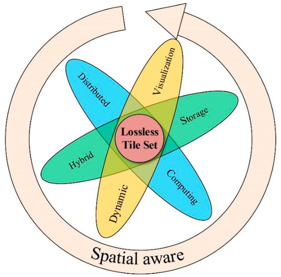
Figure 1.
Structural schematic of the SatANA framework.
2.1. Lossless Tile Set with Spatial Awareness
The lossless tile set proposed by Ye et al. [11] is the foundation of the SatANA framework. In addition, we modify the tiles by adding spatial awareness. The specific preprocessing approach of the lossless tile set includes image segmentation, resampling and compression, and finally, a lossless compressed tile set in a pyramid structure is generated. For every two adjacent levels in the pyramid, each tile in the upper level is equally divided into four lower-level tiles. As the levels go deeper, the tiles decrease until the spatial resolution is finer than that of the original image, and at this point, the maximum level is reached. Through this method, the base-of-pyramid tiles retain the complete data information of the original image and can be used for computational analyses. In addition, the pyramid structure is used to improve the speed of the real-time display and zoom of the original image, which can confer spatial awareness on the tiles.
In the SatANA framework, image segmentation is essentially a mapping between pixels (Figure 2). To preserve all the pixel values in the original image, we must map the original pixel set to a larger collection. This collection consists of several tiles that are typically 256*256 pixels. The number of tiles included in this tile set is determined by the spatial extent and resolution of the original image, and the original pixels (black pixels in Figure 2) are mapped to the new tile set by adopting the Nearest Neighborhood algorithm. In addition, regarding the undetermined pixels (red pixels in Figure 2) in the new tile set, the value is adopted from the original image by an inverse solution, and the pixel value is distinguished from the actual pixel by adding an additional digital number. Regarding the new tile set, resampling is performed using a quad-tree structure to generate a multilayer image pyramid. In addition, as the original image contains the spatial reference information and this information is lost during the tiling process, the tiles in the image pyramid adopt a TileKey technique as a spatial index. The TileKey is in a structure of (Level, X, Y). According to the built-in TileKey, the original image is serviced by tiles, which can be expressed as follows:
Similarly to the data-tiling process, the SatANA virtual globe also adopts the TileKey technology to implement the spatial placement of tiles without spatial information (Figure 3a). By parsing the arguments in the URL string of each tile and reacting based on the filename, the virtual globe can quickly determine where the tile should be placed. The level and range of the tiles to be loaded are determined by the viewpoint and distance.
f(Level,X,Y) = https:\\ServerIP Address\FileName\Level\X\Y,
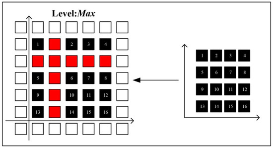
Figure 2.
Pixel mapping between tiles and the original image.
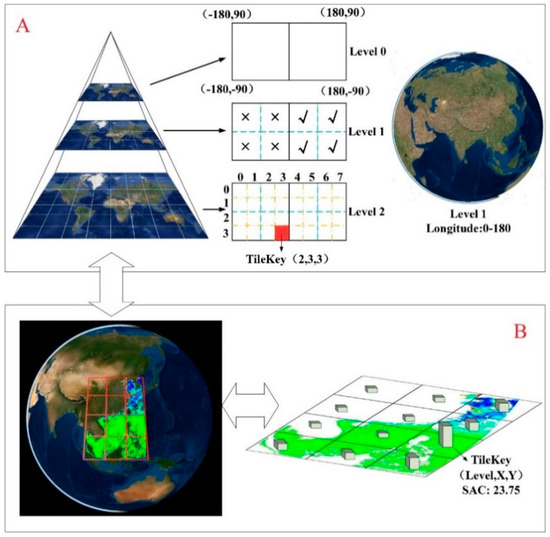
Figure 3.
Lossless tile set with spatial awareness. (A) Example of the TileKey and method used for the management of tiles with TileKey in SatANA. The current virtual earth is loaded with the tiles of Level 1 with longitude ranging from 0 to 180, that is, the ticked part. (B) Example of the Spatial Awareness Coefficient.
According to the above mechanism, we can add spatial awareness to the tiles (Figure 3b) such that not only is the placement of the tiles perceived by the SatANA virtual globe but also the loaded tiles can perceive the user’s operational behavior, thereby achieving intelligentization of the framework. According to the user’s zoom and pan operations, we define the Spatial Awareness Coefficient (SAC) of the tile as follows:
where indicates the maximum level that the original image can achieve. Thus, the deeper the level of the tile, the higher the coefficient. The zoom coefficient is the accumulation of panning. In addition, the entire coefficient of the tile is the sum of zooming and panning. All tiles in each image loaded by a user correspond to their own SAC. Furthermore, we additionally define the relationship between the node SAC and its four unzoomed child nodes SAC as follows:
where . Similarly, the relationship between the child SAC and its unzoomed parent SAC is as follows:
As the data are preprocessed, the SatANA framework can be an efficient solution for integrated and intelligent improvements in the visualization, storage and computing of MRS data, which is explained in the following section.
2.2. Tile-Based Implementation
Currently, satellite data users face challenges of volume as archives of data grow—of variety, as instruments produce finer resolution observations that must be related to existing archives to produce an on-going and consistent record, and of velocity, as the intervals between observations reduce from weeks to days, or from hours to minutes [15]. Therefore, corresponding scalable storage and fast calculation are indispensable, and the stored data and calculation results need to be vividly visualized. In this paper, we attempt to better combine and intelligently improve these issues using the above spatial-aware tile set.
2.2.1. Intelligent Hybrid Database Storage
First, as the basis for visualization and computation, the SatANA framework adopts a hybrid database storage for data organization and provides a self-tuning tile service. The concept of a hybrid database is used in many studies [16,17,18,19], but here, we improve the hybrid database by the spatial awareness of the tiles, thereby providing a more efficient tile service for visualization and distributed computing. Figure 4 shows the hybrid database storage architecture that is used to classify storage according to the data characteristics. This architecture also considers the user’s corresponding SAC information after the tiles are requested, as described in the previous section. The requested tiles are represented in the bottom left panel of Figure 4. First (top left panel of Figure 4), the in-situ data, metadata of the MRS image (including the maximum level of the pyramid structure, projection coordinates, row number, column number, spatial extent, and image statistical values) and other related structured data are managed by object-relational tables in PostgreSQL (http://www.postgresql.org), while the spatial objects of the in situ data are stored in PostGIS (https://postgis.net/). Second (top right panel of Figure 4), the massive tiles are managed by a distributed data storage approach based on the Hadoop database [20], as the high scalability of HBase provides an expanded storage capacity for increased MRS data. This part consists of an HMaster Node and several Data Nodes. The tile data are stored in the HBase tables through the HRegionServer, and the underlying layer depends on the Hadoop Distributed File System (HDFS; [21]). Third (bottom right panel of Figure 4), most importantly, we manage the real-time and large amounts of enhancement SAC information with a high-performance in-memory database. The TileKey information in SAC is GeoHashed to facilitate storage, and the writing process is completely independent of the server memory, greatly improving efficiency and protecting user privacy.
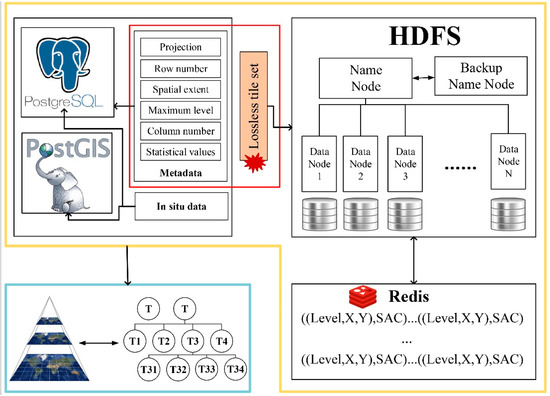
Figure 4.
Hybrid database storage architecture of classified storage according to the data characteristics. The red box in Figure 4 represents the original image.
Specifically, as shown in Figure 5, the tile request process is divided into three parts, which from left to right represent the data query in PostgreSQL, tile access in HBase, and the SAC write of the requested tile. In addition, from bottom up, the storage layer represents the hard disk of the servers, the virtual layer adopts HDFS to virtualize the cluster hard disk, the abstraction layer corresponds to the hybrid database, the exchange layer signifies the memory of the servers, and the application layer is the client. After a user queries the PostgreSQL database to select the data to be loaded, the tile requested by the user first passes through the memory, and each read triggers the corresponding SAC to write to the in-memory database.
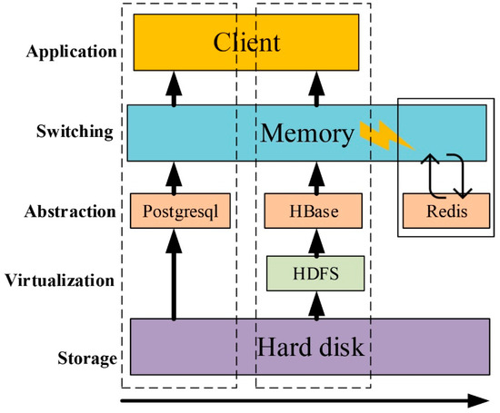
Figure 5.
Tile request process in the hybrid database storage system.
The recorded SAC is divided into real-time and historical parts. We use the SAC information to classify the heat of the tiles, which are preloaded data, hot data (data that need to be accessed frequently), and cold data (data that are accessed less frequently). The real-time SAC can obtain a relatively complete quad-tree structure, and the tiles corresponding to the children of the underlying nodes of each tree will be preloaded into the memory for immediate access, i.e., preloaded data. The historical SAC information is used to screen the heat of the data. According to the definition provided in Section 2.1, the SAC represents the degree to which users are interested in an area. The tiles corresponding to a high SAC in a certain time range are stored on solid-state drives (SSD) with better read performance for faster access. When the space of SSD is insufficient, the hybrid database calculates the weight of the tiles according to the recent access time and the access frequency and transfers the tiles with the lowest weight to normal storage. As described above, the SAC written in the process of Figure 5 can reverse the HBase optimization.
2.2.2. Dynamic Visualization Using a Virtual Globe
Although the above process is performed independently of the server, the request for data originates from the virtual globe of the client. The virtual globe technique is a new data-processing and analysis tool that can integrate heterogeneous geospatial data at the global scale [22,23]. By changing their viewing angles and positions, users can freely move around within the virtual environment provided by virtual globes, and explore and analyze geospatial information from different perspectives and at different detail levels [24]. This process generates SAC, which is not only recorded by the server but also used by the virtual globe to optimize data visualization. Visualization is described as the mapping of data to a visual form that enables researchers to cope with data by making sense of what the data actually contain when machines might fall short [25,26,27]. Regarding the rendering of marine environment elements, identifying the appropriate transfer function to map complex values into intuitive graphical image information is highly important [28]. Due to the large-scale characteristic of remote sensing, small-scale changes cannot be reflected if the transfer function is designed according to the whole image. For example, chlorophyll products in large oceanic areas are stable, while rich changes are shown in small near-shore areas. In addition, changes in different small areas may not be exactly the same; thus, we need to intelligently adjust the transfer function for user dynamics. In the SatANA framework, MRS data are displayed online in the form of pyramid tiles, and the SatANA virtual globe can dynamically design the transfer function for user-interested regions to display richer information due to the spatial-aware feature of the tiles.
Specifically, once the tiles reach the client, the image can be rendered tile-by-tile, which uses a multithreaded approach. In addition, the SatANA virtual globe dynamically updates the data that must be rendered in the memory. Thus, two queues are used for display as the tile is transferred to the user interface. One queue is the loading tile queue, which is used to retain the tiles that must be loaded. The other queue is the rendering queue. If the current tile is not in memory, it is transferred to the loading queue to prevent the loading and rendering processes from interfering with one another. Meanwhile, the SatANA virtual globe records the corresponding SAC information. Differing from the server side, the client side only records the SAC information after a restart. Due to local production and small numbers, such information is stored in a queue in memory. Based on the recorded SAC information, the framework can dynamically design the transfer function to personalize the local optimized rendering of the image. As shown in Figure 6, the pixel information of high SAC region tiles is collected to determine a suitable transfer function for local rendering, and the remaining regions use the same process to generate a uniform colorbar.
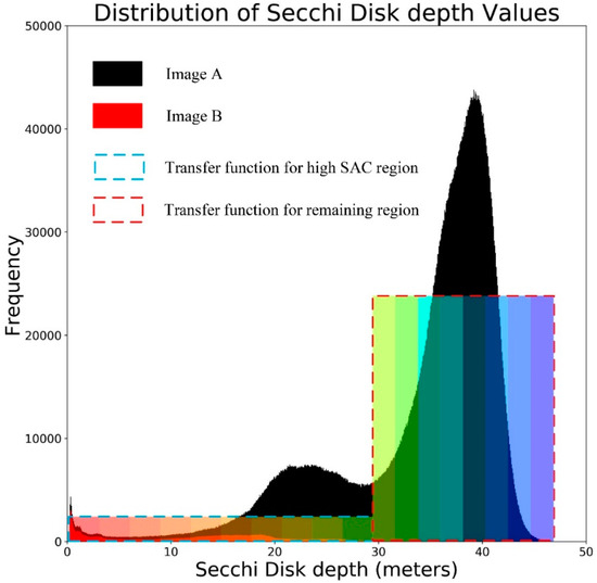
Figure 6.
Dynamical design transfer function for user-interested regions.
Specifically, suppose we have an image A with matrix in dimension m*n (, , ) whose corresponding SAC matrix is (, , ). Moreover, we have a subimage B with matrix (, , ) from image A, which is defined as follows:
where is a predetermined threshold. If we plot the histograms of image A and image B, which are called histograms (the area filled in black in Figure 6) and (the area filled in red in Figure 6), respectively, observing that is included in is trivial. Furthermore, we have a probability distribution function (pdf) for the histograms, which is , where indicates the number of times element appears in the matrix . The cumulative distribution function (cdf) can also be defined as . The pdf and cdf of histogram are defined similarly. First, we apply histogram equalization to into interval (colored rectangles surrounded by blue dotted frame in Figure 6), where , where represents the minimum nonzero value in matrix and represents the number of color gradations. Similarly, the left part in from can be equalized into interval , and the right part can be equalized into interval (colored rectangles surrounded by red dotted frame in Figure 6). Thus, the detailed transfer function for a high SAC region is as follows:
where indicates the minimum cdf on , and denotes the number of NoData elements in matrix S. In addition, the remaining transfer function for the left part in from and the right part is exactly the same. According to the resulting transfer function, we can create color filling in the data field. In addition, to achieve a gradient effect in the color field, the SatANA virtual globe adds a conversion of the RGB color space to the HSL color space by extending the Geospatial Data Abstraction Library [29] color mapping method and assigning the grid points to be drawn by the HSL model. Figure 7 shows a comparison rendering result of ocean Secchi Disk depth (SDD) between spatial aware histogram equalization (Figure 7a) and global histogram equalization (Figure 7b). The black dotted line represents a simulated high SAC area, and Figure 7a better illustrates the abundant change in seawater transparency in the nearshore area.
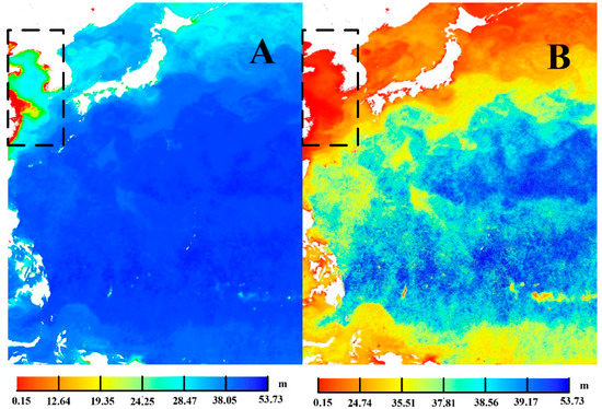
Figure 7.
Comparison of rendering results for ocean Secchi Disk depth between (A) spatial-aware histogram equalization and (B) global histogram equalization.
If users are indeed interested in the area, they will zoom in to that area, which will further enhance the area’s SAC and continue to provide a reference for the tuning of the hybrid database storage. In addition, during the visualization stage, the SatANA virtual globe caches some tiles to avoid frequent data requests. As the base-of-pyramid tiles are the lossless backup of the original data, if the user interface requests lossless-level tiles for visualization, these tiles are cached locally and can be used in subsequent basic statistical analyses.
2.2.3. SAC-Driven Hilbert Index for High-Performance Computing
In addition to basic statistical analyses, high-performance computing is required for massive MRS data. To meet the calculation and service requirements of spatiotemporal data, the SatANA framework uses a distributed parallel-processing model known as Hadoop + Spark, which integrates the spatial-aware lossless tile set technology and is available as multiple APIs for custom environments.
The distributed computing of MRS data is simplified by the Resilient Distributed Dataset (RDD) abstraction provided by Spark [30]. However, we still need to focus on the following two issues: (1) when performing distributed computing using multiple computers, there is a large demand for the timeliness of the tile index, and (2) the tiles are spatially adjacent, and thus, a suitable index is needed to inform of their mutual spatial relationship. The Hilbert curve is a commonly used spatial index that completely eliminates discontinuities compared to Quad-tree and GeoHash [31]. In the SatANA framework, we add the spatial awareness of the tiles to the Hilbert index to accelerate the entire calculation. Specifically, as shown in the definition of SAC in Section 2.1, we can obtain all the SAC information of the tiles in a loaded image. At the root level, as shown in Figure 8A, the tiles are sorted by SAC, and the tile with the highest SAC is selected as the starting point with the direction pointing to its adjacent tile, which has a higher SAC. Regarding its child nodes, we first locate the starting point in Square 1 of Figure 8A and then use the same method to locate the starting point in Square 1 of Figure 8B. The difference is that the direction here is not determined by the SAC of the adjacent tiles, but the continuity needs to be considered. If the direction points to Square 2 in Figure 8B, the curve will not be able to traverse all tiles; thus, there is no continuity. Regarding the last four tiles, we also determine the final direction based on the value of the SAC. Then, we can determine the unique Hilbert index of all tiles. When Spark requests the tiles to be calculated, the SAC-driven Hilbert index is sorted according to the degree of interest of the user, and this method can obtain the required data faster.
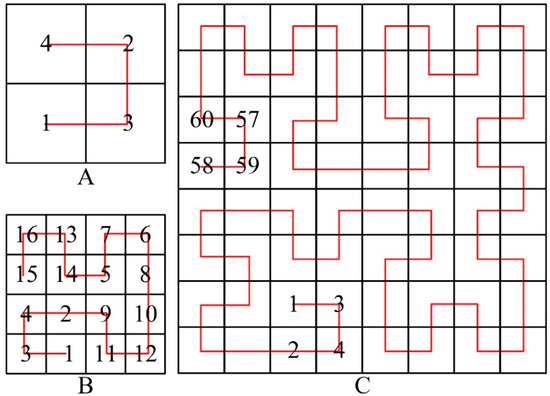
Figure 8.
Spatial Awareness Coefficient (SAC)-driven Hilbert index. (A) First-order Hilbert curve; (B) First-order Hilbert curve; (C) Third-order Hilbert curve
We conduct several experiments to demonstrate the performance of the Hadoop + Spark model with the SAC-driven Hilbert index in the following section. Additionally, the SatANA framework is adopted to a proof of concept, i.e., the SatCO2 platform, to show its superiority.
3. Platform Demonstration
To promote the sharing and multidisciplinary applications of MRS data, we developed the SatCO2 platform, which is a freely distributed piece of software adopting the SatANA framework that is devoted to meeting the needs of multisource data processing, application analyses and vivid visualization. Users can visit the SatCO2 homepage at http://www.SatCO2.com to download the installation package.
3.1. Platform Overview
The SatCO2 platform has the following two parts: a cloud data center and a user interface. The cloud data center is responsible for data storage, computing and services. The local user interface (Figure 9) is responsible for data interaction and visualization supported by the SatANA virtual globe. By connecting from the user interface to the SatCO2 cloud data center, users can utilize various forms of open data access, online displays and scientific analyses from an intuitive 3D global perspective. For example, basic statistical analyses of single MRS data, high-performance calculations of massive MRS data, interactive verification analyses between MRS and in situ data, and trend analyses of multiyear MRS data can be conducted through the SatCO2 platform. The comprehensive and characteristic long-term SatCO2 data sets hopefully offer new opportunities and possibilities for scientific research. Including raw data and products from different organizations, SatCO2 currently provides nearly 20 years of characteristic MRS data relevant to ecology and carbon cycle research. Such massive archives are unified by the SatANA hybrid database storage. A detailed description of this characteristic long-term data set is provided in Section 3.2.
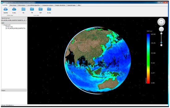
Figure 9.
User interface of SatCO2.
3.2. Online Data Sets
The SatCO2 cloud data center collect MRS data and products from different agencies, produces the data with self-developed algorithms, transforms and unifies the data formats, and uploads the final product into the SatANA hybrid database storage for online analysis applications. SatCO2 currently contains various monitoring data from seas surrounding China, the Western Pacific-Indian Ocean region and the Global Ocean over the past 20 years. Appendix A shows a detailed description of the SatCO2 online data sets. According to the data-processing characteristics, the data are divided into six categories. (1) The “Special Data Sets of the seas surrounding China” include level-1 products of the GF-4 and HY-1B satellites provided by the National Satellite Ocean Application Service of China and MRS reflectance products provided by NASA and NOAA. (2) The original data of the geostationary ocean color imager “(GOCI) Data Sets” are obtained from the GOCI level-1-B, which are geostationary ocean color satellite data provided by the Korea Ocean Satellite Center. (3) Based on the raw data of MRS reflectance products provided by NASA, SatCO2 provides surface suspended matter concentrations, chlorophyll concentrations and seawater transparency products in the Eastern Indian Ocean, Western Pacific Ocean and South China Sea in the “Western Pacific-Indian Ocean Data Sets”. (4) The “Globe Data Sets” include raw data of MRS reflectance, the total absorption coefficient and the particulate backscattering coefficient retrieved by SeaWiFS, MODIS/Aqua and VIIRS from NASA. (5) The “NASA Public Data Sets” include publicly available satellite products from NASA. (6) The “Public Data Sets of Other Institutions” include raw data from institutions, such as Remote Sensing Systems (RSS), the Copernicus Marine Environment Monitoring Service (CMEMS), Oregon State University (OSU), ESA, NOAA and the European Centre for Medium-Range Weather Forecasts (ECMWF).
These data sets are derived from 11 institutions with 10 different satellites and sensors, and the coverages spread from 1981 to the present for more than 60 products, which have formed a PB-scale storage. Due to conventional open-data policies, most data are stored and shared in the form of archives. SatCO2 made these data easy to access through the SatANA framework, which can perform online vivid visualization and carry out further efficient analyses. In addition, the SatCO2 data sets have a high spatial and temporal resolution as the SatANA framework introduces additional advantages, which are illustrated for some cases.
3.3. Case Study: Anomaly Analysis of Multiyear MRS Data
SatCO2′s advantages can be demonstrated using published studies as described in the following text. Many applications could face barriers or be prohibitively time-consuming without the advantages of the SatANA framework. By connecting to the SatCO2 cloud center, Figure 10A shows a monthly average chlorophyll concentration image in the Bay of Bengal from December 2005 obtained from the ESACCI data set at a 4 km resolution. Rendered through the SatANA virtual globe with the dynamical design transfer function for user-interested regions, a phytoplankton bloom event can be clearly observed to have occurred in the area identified within the red box. To perform phytoplankton anomaly analysis over multiple years, researchers may need to download multiple MRS data for several years and write their own analysis programs with traditional analysis methods, which is time-consuming and requires expertise. However, using SatCO2, researchers can easily perform a time series analysis of nearly 20 years of MRS data online via the Hadoop + Spark model. Specifically, by clicking to select a line on the SatANA virtual globe or importing the file identified by the longitude and latitude coordinates of the point of interest, a time series plot is automatically displayed. In Figure 10B, the white line represents the polygonal line of a time series analysis that passes through the algal bloom area. As all calculations are performed on the server, users do not need to be concerned about the computing power of their computers, and the results are immediately returned to the user interface. In Figure 10C, the x-axis represents time, and the y-axis represents the chlorophyll concentration. The dark blue dots represent the average chlorophyll concentrations in all grid points on the polygonal line, and the light blue dots represent the standard deviation of the average chlorophyll concentration in all grid points on the polygonal line. According to the results, a high chlorophyll value appeared in the southwest region of the bay in approximately December each year, and the chlorophyll concentrations in December 2005 and December 2013 were 3–4 times higher than those during normal years. Additionally, the possible causes can be examined using time-series data sets of satellite-derived sea surface height anomalies, sea surface temperatures, wind stress and Ekman pumping velocity data [32], which can also be supplied by SatCO2 using the SatANA framework.
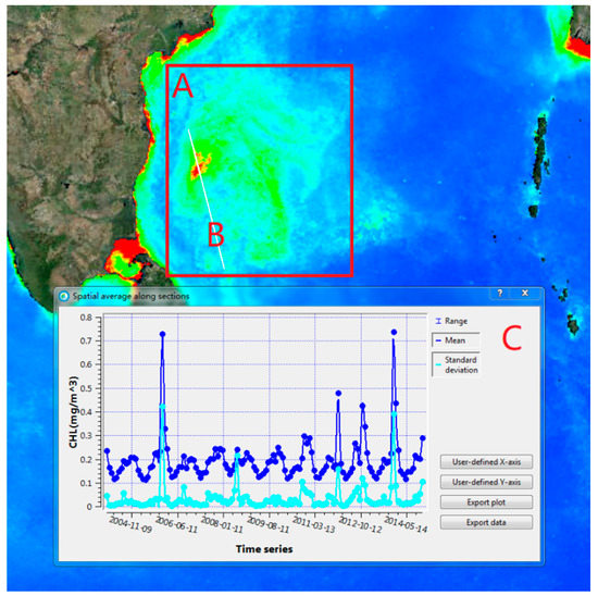
Figure 10.
Diagram of the spatial average along a section of chlorophyll concentration.
3.4. Calculation Ability: Satellite-Driven Ocean SDD Retrieval
The SatANA framework not only facilitates easy online analyses but also provides improvements in computing performance. In this section, we perform a more complex multiyear retrieval of satellite-driven ocean SDD to show the potential of the SatCO2 platform and the calculation ability promotion of the SatANA framework. The SDD is widely used to indicate water transparency [33]. In traditional in situ SDD measurements, seasonal and interannual variations and long-term changes in ocean transparency at the global scale remain poorly understood. However, in recent decades, satellite ocean color remote sensing has made it possible to observe the daily global SDD [34]. The SDD can be retrieved using a semi-analytic algorithm [35,36,37] as follows:
where and are the total absorption and particulate backscattering coefficients at 443 nm, respectively, and is the remote sensing reflectance at 443 nm. In this section, we use the SeaWiFS data, which have a global coverage and a spatial resolution of 9 km, for SDD retrieval. To verify the accuracy of the satellite-retrieved SDD, we use the global in situ SDD data obtained from the Worldwide Ocean Optics Database (WOOD) [38] from September 1997 to November 2010. Similarly, the SeaWiFS data are also derived during this time period. Then, we perform one-to-one matching according to the latitude and longitude information. Figure 11 shows the schematic flow.
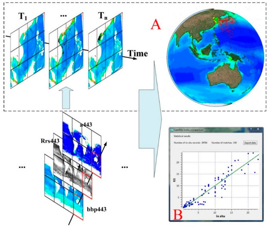
Figure 11.
(A) Spatiotemporal Secchi Disk depth (SDD) data with the red points indicating the in situ samples. (B) Scatter diagram comparing the matched points of the satellite-retrieved SDD and Worldwide Ocean Optics Database (WOOD) in situ data. The x-axis represents the in situ data, and the y-axis represents the MRS data. The dark green line represents the 1:1 line.
The processing speed of the remote sensing image is determined by the following two factors: the number of image pixels and the complexity of the processing algorithm [39]. Notably, the size of one day of SeaWiFS raw data is approximately 5 MB, and the size of all data covering WOOD’s full time is approximately 24 GB. This size represents the compressed size in the NetCDF format, although the actual size of the full data is approximately 506 GB as calculated according to a 32-bit float per pixel. Moreover, there are 29,784 samples in the in situ data. Specifically, 29,784 loops with multiple checks are required, representing a large workload. By testing in an experimental cluster of the same hardware environment, Figure 12 shows the resulting improved efficiency of this process under the SatANA framework. The blue and orange histograms represent the time cost of accelerating with or without the Spark framework. The gray histogram shows the time cost using the SatANA framework. Based on the speedup lines, the retrieval of the satellite-driven SDD can be observed, and the SatANA framework has a perceptible computational efficiency improvement. Specifically, in this case, the most time-consuming part of this process is the data reading. The SatANA framework, which deeply integrates existing resources, is a useful method for avoiding this drawback. First, the intermediate output in Spark can be stored in memory, eliminating the need to frequently read and write on the local file system. Second, the lightweight tiles are easier to read, further improving the comparison efficiency. Moreover, the SAC-driven Hilbert index can shorten the indexing time of the requested data; however, in this case, it is not significant as global data are involved.
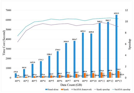
Figure 12.
Time cost comparison of multiyear satellite-driven SDD retrieval using different computing methods with a fixed hardware configuration.
3.5. Application: Training Courses
The above example confirms the convenience and improvement of SatCO2, and we hope to help more researchers with their studies. Several SatCO2 training courses were successfully held from 2018 to 2019 as follows:
- In November 2018, a SatCO2 training course was held at the Dragon 4 Cooperation Program in Shenzhen, China;
- In November 2018, the SatCO2-III workshop was held in Hangzhou, China;
- In April 2019, a SatCO2 training course was held at the International Ocean Color Science Meeting in Busan, South Korea;
- In April 2019, a SatCO2 training course was held at the 4th Global Ocean Acidification Observing Network International Workshop in Hangzhou, China;
- In October 2019, an advanced training course on ocean color remote sensing was held in Hangzhou, China. In addition, the participants learned to use SatCO2 for environmental monitoring and scientific research.
The multi-user simultaneous access during the training courses had greater stress and better randomness, which is not possible with daily use and self-simulation. Thus, we recorded the average tile read time of the hybrid database storage during the training courses to verify its advancement. Considering the different client network conditions, we only record the tile read time on the server side. Figure 13 shows a typical result during one training session with about 80 trainers. As shown, the average tile read time sharply increases and then gradually decreases. We postulate that the reason why the tile read time sharply increases is because the training is divided into the following two parts: practical teaching and self-operation. During the practical teaching process, everyone loads the same set of tiles, and there is a cache situation; thus, the average reading time reaches a low point. However, subsequently, as the trainees operate on their own, the hybrid database storage gradually reduces the data read time by recording the SAC and dynamically tuning the tile service.
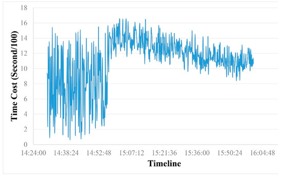
Figure 13.
Average tile read time during a training course.
4. Challenges and Further Work
Although the SatANA framework has made integrated and intelligent improvements to existing technologies and is capable of more effectively managing and utilizing MRS data, it also has several shortcomings. First, the massive MRS data are processed into a high number of smaller tiles, causing data redundancy. Second, the capabilities of the SatANA Hadoop + Spark model have not been fully utilized to date. Considering the popularity of relatively recent concepts, such as neural networks and deep learning, determining how to combine the SatANA framework with current international cutting-edge technology is a concern. Third, the SatANA framework is primarily applicable to two-dimensional data. For three-dimensional data, such as profiles, a proper management and visualization method is lacking. We think that three-dimensional profile data in the SatANA framework are not simply two-dimensional data with an additional time or depth dimension. There should be a more efficient way to manage such data for visualization and computational use. We will continue to improve the SatANA framework to improve its efficiency and increase its applicability.
Another issue is that SatCO2, i.e., the platform that adopts the SatANA framework to achieve high availability for easy access and efficient analyses of MRS data, also has certain limitations and requires further development. First, raw data acquisition is limited. Currently, there are two main sources of the original MRS data used in the SatCO2 data center as follows: data received by the National Marine Satellite Ground Station of China (Hangzhou) and data downloaded from other agencies. The National Marine Satellite Hangzhou Ground Station is one of the four major ground stations for marine satellite operational applications in China. The Level-1 data of the Chinese satellite HY-1B in the SatCO2 data sets are also provided by the Hangzhou ground station. However, the other data are collected from many types of agencies and are distributed after processing. Although most processes are automatically completed by the software, they still require manual downloading, which can cause data update delays. Therefore, we hope to cooperate with the data providers to achieve automatic data acquisition and updates in future. Second, there are certain deficiencies in the stability and computing responsiveness of SatCO2. For stability, after the public beta of the above training courses, SatCO2 is constantly being improved, and we will continue to launch new versions in the future to fix its bugs and add new functions. For the response efficiency, we are currently gradually migrating existing data to the self-built Lin’an data center. The number of cloud servers is six times that of the existing data centers. The architecture of the Lin’an cloud data center has also been redesigned, and the processing speed will be qualitatively improved. Third, another challenge is related to the limited professional modules. For marine monitoring applications, complex processes are involved. In addition to its visualization and computational analysis functions, SatCO2 integrates professional modules for specialized applications. In the current version, we integrated air-sea CO2 flux estimation, bloom monitoring, and water quality classification modules for marine acidification, marine environmental protection and marine ecological disaster warning. We hope to collaborate with other researchers to develop new algorithms and models and fully explore the potential of the SatANA framework.
5. Conclusions
The objective of this paper is to propose an intelligent tile-based framework for easy access to and efficient analyses of MRS data. The spatial-aware tile combining cutting-edge technology helps narrow the gap between MRS archives and end users. Specifically, compared to the original image, the tile set is easier to transmit over the web, allowing users to browse these resources online, and its distribution characteristics have a spatial-aware advantage. The behavior of the user while roaming and browsing data can help the SatANA virtual globe to dynamically adjust the rendering transfer function to achieve a more user-expected effect. In addition, as the data are requested from the server side, this behavior is also independently recorded on the hybrid database storage, allowing for reverse optimization while preserving user privacy and further providing the more efficient SAC-driven Hilbert index for the Hadoop + Spark computing model. Such an approach can substantially enhance the user experience by integrating online data access, high-performance calculations, and 3D visualizations for tracking, monitoring, understanding and communicating environmental changes.
By focusing on international research issues, such as the ocean carbon cycle and ocean acidification, we apply the SatANA framework to the SatCO2 platform, which is devoted to being helpful in long-sequence quantitative remote sensing science in fields such as marine chemistry, marine biology, ocean dynamics and ocean remote sensing. To the best of our knowledge, SatCO2 is one of the few platforms used for online applications of analyses of remote sensing data. The most similar applications include Google’s Earth Engine and NASA’s Giovanni. Compared with Earth Engine, the underlying data support for both is based on tiles. The remote sensing images are pre-processed into tiles in the image’s original projection and resolution and stored in an efficient tile database for quick and efficient access. They both build an image pyramid to achieve fast online visualization. The difference is that, based on the distribution characteristics of tiles, SatCO2 further adopts the spatial-aware feature of tiles to improve the user experience. Additionally, from a platform perspective, SatCO2 focuses on the application of satellite remote sensing in marine research and offers a more characteristic data set. The data are produced based on our latest research findings and algorithms for more intuitive products and user experiences, which makes it easy for individuals who lack remote sensing backgrounds to use the application. In comparison, Giovanni is a web service workflow-based system [40] with highly limited functionality. In addition, Giovanni does not facilitate interactive analyses of remote sensing and in situ data. As an online analysis platform for MRS data, SatCO2 meets the needs of users at different levels and can be a convenient tool for research.
Author Contributions
Conceptualization, W.Y., F.Z., X.H., Y.B. and Z.D.; investigation, W.Y.; methodology, W.Y.; validation, W.Y., Z.D. and F.Z.; formal analysis, W.Y. and Y.B; data curation, X.H. and Y.B.; writing—original draft preparation, W.Y.; writing—review and editing, W.Y., Z.D., F.Z. and Y.B; supervision, Z.D.; funding acquisition, Z.D. and R.L. All authors have read and agreed to the published version of the manuscript.
Funding
This research was supported by the National Key Research and Development Program of China [2016YFC1400903,2018YFB0505000], the National Natural Science Foundation of China [41671391,41871287], and the Public Science and Technology Research Funds Projects for Ocean Research [201505003].
Acknowledgments
The SatCO2 platform was developed by the State Key Laboratory of Satellite Ocean Environment Dynamics (SOED) of the Second Institute of Oceanography of the State Oceanic Administration and the Zhejiang Provincial Key Laboratory of Resources and Environmental Information System. The online data services are provided by the RS Data Sharing Center of the National Key Laboratory of SOED. The SMAP salinity data are produced by RS Systems and sponsored by the NASA Ocean Salinity Science Team. The data are available at www.remss.com. The WindSat data are produced by RS Systems and sponsored by the NASA Earth Science MEaSUREs DISCOVER Project and the NASA Earth Science Physical Oceanography Program. The RSS WindSat data are available at www.remss.com. The CCMP Version-2.0 vector wind analyses are performed by RS Systems. The data are available at www.remss.com. The Net Primary Production data are provided by the Ocean Productivity site (http://www.science.oregonstate.edu/ocean.productivity/index.php). Ocean Colour Climate Change Initiative dataset, Version 3.1, European Space Agency is available online at http://www.esa-oceancolour-cci.org/. Global sea level anomalies, mixed layer thickness/depth, and model results of geostrophic flow are provided by the Copernicus Marine Environment Monitoring Service. The Level-1B data of the geostationary ocean color imager are provided by the Korean Ocean Satellite Center. The Level-1 data of the Chinese satellite HY-1B are provided by the national marine satellite ground station of China (Hangzhou), SOED/SIO. The Level-1 data of the Chinese satellite GaoFen-4 are provided by National Satellite Ocean Application Service of China.
Conflicts of Interest
The authors declare no conflict of interest.
Appendix A

Table A1.
Online data sets on the SatCO2 platform.
References
- Berger, M.; Moreno, J.; Johannessen, J.A.; Levelt, P.F.; Hanssen, R.F. ESA’s sentinel missions in support of Earth system science. Remote Sens. Environ. 2012, 120, 84–90. [Google Scholar] [CrossRef]
- Han, G.; Chen, J.; He, C.; Li, S.; Wu, H.; Liao, A.; Peng, S. A web-based system for supporting global land cover data production. ISPRS J. Photogramm. Remote Sens. 2015, 103, 66–80. [Google Scholar] [CrossRef]
- Boyd, D.S.; Jackson, B.; Wardlaw, J.; Foody, G.M.; Marsh, S.; Bales, K. Slavery from space: Demonstrating the role for satellite remote sensing to inform evidence-based action related to UN SDG number 8. ISPRS J. Photogramm. Remote Sens. 2018, 142, 380–388. [Google Scholar] [CrossRef]
- Ma, Y.; Wu, H.; Wang, L.; Huang, B.; Ranjan, R.; Zomaya, A.; Jie, W. Remote sensing big data computing: Challenges and opportunities. Future Gener. Comput. Syst. 2015, 51, 47–60. [Google Scholar] [CrossRef]
- Peternier, A.; Boncori, J.P.M.; Pasquali, P. Near-real-time focusing of ENVISAT ASAR Stripmap and Sentinel-1 TOPS imagery exploiting OpenCL GPGPU technology. Remote Sens. Environ. 2017, 202, 45–53. [Google Scholar] [CrossRef]
- Liu, Q.; Klucik, R.; Chen, C.; Grant, G.; Gallaher, D.; Lv, Q.; Shang, L. Unsupervised detection of contextual anomaly in remotely sensed data. Remote Sens. Environ. 2017, 202, 75–87. [Google Scholar] [CrossRef]
- Mattmann, C.A. Computing: A vision for data science. Nature 2013, 493, 473–475. [Google Scholar] [CrossRef]
- Wang, L.; Ma, Y.; Yan, J.; Chang, V.; Zomaya, A.Y. pipsCloud: High performance cloud computing for RS big data management and processing. Future Gener. Comput. Syst. 2018, 78, 353–368. [Google Scholar] [CrossRef]
- Gorelick, N.; Hancher, M.; Dixon, M.; Ilyushchenko, S.; Thau, D.; Moore, R. Google Earth Engine: Planetary-scale geospatial analysis for everyone. Remote Sens. Environ. 2017, 202, 18–27. [Google Scholar] [CrossRef]
- Yu, L.; Gong, P. Google Earth as a virtual globe tool for Earth science applications at the global scale: Progress and perspectives. Int. J. Remote Sens. 2012, 33, 3966–3986. [Google Scholar] [CrossRef]
- Ye, W.; Zhang, F.; Bai, Y.; Du, Z.; Liu, R. A tile service-driven architecture for online climate analysis with an application to estimation of ocean carbon flux. Environ. Model. Softw. 2019, 118, 120–133. [Google Scholar] [CrossRef]
- Fu, G. SeaDAS: The SeaWiFS data analysis system. In Proceedings of the PORSEC’98, Qingdao, China, 28–31 July 1998; pp. 73–79. [Google Scholar]
- Zhang, T.; Li, J.; Liu, Q.; Huang, Q. A cloud-enabled remote visualization tool for time-varying climate data analytics. Environ. Model. Softw. 2016, 75, 513–518. [Google Scholar] [CrossRef]
- Giuliani, G.; Dao, H.; De Bono, A.; Chatenoux, B.; Allenbach, K.; De Laborie, P.; Rodila, D.; Alexandris, N.; Peduzzi, P. Live Monitoring of Earth Surface (LiMES): A framework for monitoring environmental changes from Earth Observations. Remote Sens. Environ. 2017, 202, 222–233. [Google Scholar] [CrossRef]
- Lewis, A.; Oliver, S.; Lymburner, L.; Evans, B.; Wyborn, L.; Mueller, N.; Raevski, G.; Hooke, J.; Woodcock, R.; Sixsmith, J.; et al. The Australian geoscience data cube—Foundations and lessons learned. Remote Sens. Environ. 2017, 202, 276–292. [Google Scholar] [CrossRef]
- Goyal, S.; Srivastava, P.P.; Kumar, A. An overview of hybrid databases. In Proceedings of the 2015 International Conference on Green Computing and Internet of Things (ICGCIoT), Noida, India, 8–10 October 2015. [Google Scholar]
- Villari, M.; Giacobbe, M.; Fazio, M. Enriched ER model to design hybrid database for big data solutions. In Proceedings of the 2016 IEEE Symposium on Computers and Communication (ISCC), Messina, Italy, 27–30 June 2016. [Google Scholar]
- Ogasawara, G.H.; Tso, M.M. Hybrid Data Management System and Method for Managing Large, Varying Datasets. U.S. Patent No. 9,396,290, 19 July 2016. [Google Scholar]
- Vyawahare, H.R.; Karde, P.P.; Thakare, V.M. A Hybrid Database Approach Using Graph and Relational Database. In Proceedings of the 2018 International Conference on Research in Intelligent and Computing in Engineering (RICE), San Salvador, El Salvador, 22–24 August 2018. [Google Scholar]
- Vora, M.N. Hadoop-HBase for large-scale data. In Proceedings of the 2011 International Conference on Computer Science and Network Technology, Harbin, China, 24–26 December 2011; Volume 1. [Google Scholar]
- Fortner, B. HDF: The hierarchical data format. Dr. Dobb’s J. Softw. Tools Prof. Program. 1998, 23, 42. [Google Scholar]
- Shupeng, C.; van Genderen, J. Digital Earth in support of global change research. Int. J. Digit. Earth 2008, 1, 43–65. [Google Scholar]
- Liu, P.; Gong, J.; Yu, M. Visualizing and analyzing dynamic meteorological data with virtual globes: A case study of tropical cyclones. Environ. Model. Softw. 2015, 64, 80–93. [Google Scholar] [CrossRef]
- Zhu, L.; Chen, X.; Li, Z. Multiple-view geospatial comparison using web-based virtual globes. ISPRS J. Photogramm. Remote Sens. 2019, 156, 235–246. [Google Scholar] [CrossRef]
- Hoffer, D. What does Big Data Look Like? Visualization is Key for Humans. Available online: http://www.wired.com/insights/2014/01/big-data-look-like-visualization-k (accessed on 12 February 2020).
- Li, S.; Dragicevic, S.; Castro, F.A.; Sester, M.; Winter, S.; Coltekin, A.; Pettit, C.; Jiang, B.; Haworth, J.; Stein, A.; et al. Geospatial big data handling theory and methods: A review and research challenges. ISPRS J. Photogramm. Remote Sens. 2016, 115, 119–133. [Google Scholar] [CrossRef]
- Integrating geo web services for a user driven exploratory analysis. ISPRS J. Photogramm. Remote Sens. 2016, 114, 294–305.
- Fang, S.; Biddlecome, T.; Tuceryan, M. Image-based transfer function design for data exploration in volume visualization. In Proceedings of the Visualization’98 (Cat. No. 98CB36276), Research Triangle Park, NC, USA, 18–23 October 1998. [Google Scholar]
- Warmerdam, F. The geospatial data abstraction library. In Open Source Approaches in Spatial Data Handling; Springer: Berlin, Heidelberg, 2008; pp. 87–104. [Google Scholar]
- Salloum, S.; Dautov, R.; Chen, X.; Peng, P.X.; Huang, J.Z. Big data analytics on Apache Spark. Int. J. Data Sci. Anal. 2016, 1, 145–164. [Google Scholar] [CrossRef]
- Jiang, H.; Kang, J.; Du, Z.; Zhang, F.; Huang, X.; Liu, R.; Zhang, X. Vector spatial big data storage and optimized query based on the multi-level Hilbert grid index in HBase. Information 2018, 9, 116. [Google Scholar] [CrossRef]
- Chen, X.; Pan, D.; Bai, Y.; He, X.; Chen, C.T.A.; Hao, Z. Episodic phytoplankton bloom events in the Bay of Bengal triggered by multiple forcings. Deep Sea Res. Part I Oceanogr. Res. Pap. 2013, 73, 17–30. [Google Scholar] [CrossRef]
- Prasad, K.S.; Bernstein, R.L.; Kahru, M.; Michell, B.G. Ocean color algorithms for estimating water clarity (Secchi depth) from SeaWiFS. J. Adv. Mar. Sci. Technol. Soc. 1998, 4, 301–306. [Google Scholar]
- He, X.; Pan, D.; Bai, Y.; Wang, T.; Chen, C.T.A.; Zhu, Q.; Gong, F. Recent changes of global ocean transparency observed by SeaWiFS. Cont. Shelf Res. 2017, 143, 159–166. [Google Scholar] [CrossRef]
- He, X.Q.; Pan, D.L.; Mao, Z.H. Water transparency (Secchi depth) monitoring in the China Sea with the SeaWiFS satellite sensor. In Remote Sensing for Agriculture, Ecosystems and Hydrology VI; International Society for Optics and Photonics: Canary Islands, Spain, 2004; Volume 5568, pp. 112–122. [Google Scholar] [CrossRef]
- Jiao, N.Z.; Zhang, Y.; Zeng, Y.; Gardner, W.D.; Mishonov, A.V.; Richardson, M.J.; Hong, N.; Pan, D.; Yan, X.-H.; Jo, Y.-H.; et al. Ecological anomalies in the East China Sea: Impacts of the Three Gorges Dam? Water Res. 2007, 41, 1287–1293. [Google Scholar] [CrossRef]
- Doron, M.; Babin, M.; Hembise, O.; Mangin, A.; Garnesson, P. Ocean transparency from space: Validation of algorithms estimating Secchi depth using MERIS, MODIS and SeaWiFS data. Remote Sens. Environ. 2011, 115, 2986–3001. [Google Scholar]
- Smart, J.H. Worldwide Ocean Optics Database (WOOD); Johns Hopkins University Applied Physics Lab: Laurel, MD, USA, 2002. [Google Scholar]
- Wang, P.; Wang, J.; Chen, Y.; Ni, G. Rapid processing of RS images based on cloud computing. Future Gener. Comput. Syst. 2013, 29, 1963–1968. [Google Scholar] [CrossRef]
- Berrick, S.W.; Leptoukh, G.; Farley, J.D.; Rui, H. Giovanni: A web service workflow-based data visualization and analysis system. IEEE Trans. Geosci. RS 2008, 47, 106–113. [Google Scholar] [CrossRef]
- NASA Goddard Space Flight Center, Ocean Ecology Laboratory, Ocean Biology Processing Group. Sea-Viewing Wide Field-of-View Sensor (SeaWiFS), Moderate-Resolution Imaging Spectroradiometer on Board Aqua (MODIS/Aqua), Visible Infrared Imaging Radiometer (VIIRS), Ocean Color Data, NASA OB.DAAC. 2018. Available online: https://doi.org/10.5067/ORBVIEW-2/SEAWIFS_OC.2014.0 (accessed on 29 February 2020).
- Research Data Archive at the National Center for Atmospheric Research. Computational and Information Systems Laboratory. Available online: https://doi.org/10.5065/D6M043C6 (accessed on 9 November 2018).
- Takahashi, T.; Sutherland, S.C.; Kozyr, A. Global Ocean Surface Water Partial Pressure of CO2 Database: Measurements Performed During 1957–2015 (Version 2015); ORNL/CDIAC-161, NDP-088(V2015); Carbon Dioxide Information Analysis Center, Oak Ridge National Laboratory, U.S. Department of Energy: Oak Ridge, TN, USA, 2016. [CrossRef]


© 2020 by the authors. Licensee MDPI, Basel, Switzerland. This article is an open access article distributed under the terms and conditions of the Creative Commons Attribution (CC BY) license (http://creativecommons.org/licenses/by/4.0/).