The Infrared Absolute Radiance Interferometer (ARI) for CLARREO

Abstract

The Absolute Radiance Interferometer (ARI) is an infrared spectrometer designed to serve as an on-orbit radiometric reference with the ultra-high accuracy (better than 0.1 K 3-σ or k = 3 brightness temperature at scene brightness temperature) needed to optimize measurement of the long-term changes of Earth’s atmosphere and surface. If flown in an orbit that frequently crosses sun-synchronous orbits, ARI could be used to inter-calibrate the international fleet of infrared (IR) hyperspectral sounders to similar measurement accuracy, thereby establishing an observing system capable of achieving sampling biases on high-information-content spectral radiance products that are also <0.1 K 3-σ. It has been shown that such a climate observing system with <0.1 K 2-σ overall accuracy would make it possible to realize times to detect subtle trends of temperature and water vapor distributions that closely match those of an ideal system, given the limit set by the natural variability of the atmosphere. This paper presents the ARI sensor’s overall design, the new technologies developed to allow on-orbit verification and test of its accuracy, and the laboratory results that demonstrate its capability. In addition, we describe the techniques and uncertainty estimates for transferring ARI accuracy to operational sounders, providing economical global coverage. Societal challenges posed by climate change suggest that a Pathfinder ARI should be deployed as soon as possible.

1. Introduction

Since 1959, when the first instrument to view the Earth from space using omni-directional black, white, and gold hemispherical detectors was flown on Explorer VII by Verner Suomi and Robert Parent from the University of Wisconsin, it has been widely recognized that the global perspective of satellites is invaluable for exploring how the climate system of the Earth operates. This first sensor to explore the Earth radiation budget and establish a good estimate of its albedo, and many follow-on sensors that helped understand the radiative effect of clouds and key radiative feedbacks (Suomi/Parent hemispheres on TIROS and flat plates on ESSA 3/5/7/9, ITOS-1 and NOAA-1 satellites; ERB on Nimbus-7; ERBE on ERBS and NOAA satellites; and CERES on TRMM, EOS, and JPSS) have been based on observing the integrated effect of both solar heating and cooling from infrared emission.

While much has been learned from this total, integrated band approach, the virtue and practicality of measuring more detailed spectral properties of the radiance field became recognized in the late 1980s and led to proposals for spectrally resolved radiation budget experiments from Jim Hansen at NASA GISS (CLIMSAT in 1993 [1]) and Jim Anderson at Harvard (Arrhenius in 1996, [2]). The idea of both was to achieve much higher information content than possible with broad integrated spectral channel measurements that provided a basic calorimetry experiment. Also, Jim Anderson added (1) the element of emphasizing absolute accuracy, proven on-orbit, to replace reliance on the overlap of subsequent measurement systems to establish long-term trends and (2) the importance of multiple, carefully chosen orbits to reduce spatial and temporal biases to acceptable levels [3].

These proposals benefited from earlier hyperspectral sounder developments aimed at improving the temperature, water vapor, and trace gas profiling capability of future geosynchronous Earth orbit (GEO) and low Earth orbit (LEO) operational sensors for weather and atmospheric chemistry. In the 1980s, our group at the University of Wisconsin developed an accurately calibrated Fourier Transform Spectrometer (FTS), the High-resolution Interferometer Sounder (HIS), for flight on the high-altitude NASA U2/ER2 aircraft [4,5]. The initial goal of HIS was to demonstrate the factor-of-3 increase in profile vertical resolution expected in moving from filter radiometer sounders to hyperspectral sounders capable of resolving individual atmospheric absorption lines. In addition to achieving this goal, HIS somewhat unexpectedly demonstrated the high degree of accuracy attainable with a spectrometer [6,7] that naturally reduces the often dominant component of radiometric error stemming from uncertainty in the spectral scale and unresolved spectral properties [8].

The high accuracy of spectra from HIS soon attracted the attention of Tony Clough, author of the Fast Atmospheric Signature Code (FASCODE) line-by-line radiative transfer model, who quickly recognized their value for improving spectroscopy. Ultimately, this led to the development of a highly accurate up-looking spectrometer, the University of Wisconsin Atmospheric Emitted Radiance Interferometer (AERI) under the Department of Energy (DOE) Atmospheric Radiation Measurement (ARM) Program in the 1990s [9,10]. Further, the ARM program supported the design of a new aircraft instrument, the Scanning-HIS [11], which also demonstrated high accuracy by comparison to National Institute of Standards and Technology (NIST) standards, and has been successfully flown in many National Aeronautics and Space Administration (NASA), National Oceanic and Atmospheric Administration (NOAA), and DOE missions on five different aircraft platforms since 1998. Recognition of the value of highly accurate spectrometers for the climate as well as for weather applications was growing.

To emphasize the accuracy advantage of high spectral resolution measurements for climate, it is interesting to compare the accuracy normally specified for the total integrated infrared flux of conventional climate measurements like those from the Clouds and the Earth’s Radiant Energy System (CERES). A typical flux uncertainty threshold specification that has proven to be a challenge to meet is a percent flux uncertainty of less than 0.5% k = 1. For comparison to the brightness temperature specification we use for hyperspectral measurements, it is easy to show that a change of 0.325 K is needed to create such an 0.5% flux change for a 260 K source. Therefore, the conventional climate measurement accuracy performance for k = 3 is an order of magnitude worse than the <0.1 K k = 3 brightness temperature at scene temperature performance of the Absolute Radiance Interferometer (ARI).

In 2004, we joined forces with the Anderson Group at Harvard to promote a new climate observing initiative. Our concept was introduced at the multi-agency workshop entitled Achieving Satellite Instrument Calibration for Climate Change (ASIC³) [12]. Then, as part of the first National Research Council (NRC) Earth science Decadal Survey in 2007 [13], the Climate Absolute Radiance and Refractivity observatory (CLARREO) was named a Tier 1 mission. Soon thereafter, NASA Langely Research Center (LaRC) was chosen to carry out the mission, and the University of Wisconsin-Madison Space Science and Engineering Center teamed with Harvard and ABB, Quebec was awarded a NASA Instrument Incubator Program for the development of the ARI as the CLARREO IR spectrometer.

This is the background that led to the development of the ARI. The rest of the paper is organized as follows: Section 2 summarizes the CLARREO program and the ARI connection, followed by a top-level description of ARI in Section 3, details of its Calibrated FTS in Section 4, the On-orbit Verification and Test System in Section 5, and finally a discussion of how ARI can be used to inter-calibrate the fleet of operational hyperspectral sounders in Section 6. Section 7 presents conclusions.

2. CLARREO

The CLARREO mission was defined to provide a long-term, global record that is not only highly sensitive to climate forcing and feedback mechanisms, but also highly accurate, tested for systematic errors on-orbit, and tied to irrefutable standards. It is aimed at establishing a series of benchmarks for decadal climate tending. The benchmarks need to be repeated periodically (say every decade), but because of their proven, high accuracy do not need to overlap. Each benchmark does need to extend for an order of 5 years to average over natural variability. An observing system simulation experiment (OSSE) based on 100 years of all-sky climate model data has demonstrated that such a record of benchmark radiance data can be used to accurately define long-term trends in geophysical properties that will be highly useful in improving climate forecast models [14].

As described in Wielicki et al., 2013 [15], CLARREO includes three types of benchmark measurements that, after some exciting new technology developments, have been proven capable of meeting these demanding objectives. The first, the topic of this paper, is the spectrally resolved infrared radiance (IR) emitted from Earth to space determined with an accuracy of 0.1 K (k = 3, or 99% confidence) [16]. The infrared spectra are traced to the SI standard for the Kelvin through the Planck function theory. The second benchmark is the phase delay rate of the signal from the low-Earth-orbit Global Positioning System radio occultation system (GPS-RO) with an accuracy of 0.1% (k = 3) for 5 to 20 km in the atmosphere, traced to the SI standard for the second. The third benchmark measurement is spectrally resolved nadir reflectance of solar radiation (RS) from Earth to space determined with an accuracy of 0.5% (k = 3), relative to the mean spectral reflectance of the Earth traced to the Watt using solar spectral irradiance observations from Total Solar Irradiance Spectrometer (TSIS). The CLARREO science team has also demonstrated that, for climate products, each of these measurements is valuable in its own right and does not need to be flown on the same spacecraft.

Under NASA support, the scientific rationale for the CLARREO mission was robustly formulated by a very capable science team in the time frame from 2008 to 2015. However, despite a successful Mission Confirmation Review in 2010, the funding for further mission development was unfortunately terminated in 2011, and the full CLARREO mission as described in Wielicki et al. [15] no longer has mission status at NASA. Currently, the development of a reflected solar (RS) demonstration is continuing as a CLARREO Pathfinder mission, and GPS-RO observations are being pursued by NOAA and other countries. While funding for an IR Pathfinder was originally included in the 2016 president’s budget along with the RS Pathfinder, support for the IR has not been consummated.

A pathfinder mission for the IR is especially attractive at this time, because advances in the operational hyperspectral sounder network make such a mission very cost effective. In the near future there will be a hyperspectral sounder in the 0530 orbit when FY3E is launched with the Hyperspectral Infrared Atmospheric Sounder (HIRAS) instrument (proven on FY3D). HIRAS will join the mature joint EUMETSAT/NOAA system currently consisting of three Infrared Atmospheric Sounding Interferometer (IASI) instruments on MetOp at 0930, and two Cross-track Infrared Sounder (CrIS) instruments at 1330 on Suomi NPP and NOAA20. Therefore, the flight of a single ARI in an opportune orbit would provide the means to convert this fleet of weather sounding instruments into a CLARREO-like climate benchmarking system with excellent global coverage, provided sufficient stability of the operational fleet of infrared sounders and an adequate inter-calibration period. Flying ARI in a precessing orbit like that of the 52-degree inclination ISS, or a non-precessing, true polar, orbit would provide the opportunity to inter-calibrate all of the operational sounders to the high accuracy of ARI, proven on-orbit (see Section 6 and Tobin et al. [17]), thereby allowing a highly accurate global benchmark to essentially begin immediately. Extensive overlapping high spectral resolution infrared datasets for the 0930 and 1330 local equator crossing time sun-synchronous orbits have been provided by CrIS, IASI, and AIRS (Atmospheric Infrared Sounder) since 2012, and IASI and AIRS since 2006. Extensive intercomparisons of these datasets have been conducted as part of the international GSICS (Global Space-based Inter-Calibration System) effort and the results have shown the sensors to have excellent stability and agreement over their common mission lifetimes. Thus, it is reasonable to expect that, with somewhat larger error bars, this benchmark could even be extended significantly backward in time. The only major limitation of this benchmark would be that only ARI itself would provide far-infrared (FIR) coverage from 16 to 50 microns; however, the operational sounders are designed to give excellent information content on profiles of temperature and water vapor, clouds, surface properties, and even trace gases.

So why is it reasonable to think that a relatively inexpensive instrument for climate can improve the accuracy (as well as spectral coverage) of the sophisticated operational hyperspectral sounders of today? The rest of this paper will give a detailed answer to this question, but it seems worthwhile to provide a simple general explanation before getting into the details. Part of the answer is contained in

Table 1. The Climate Absolute Radiance and Refractivity observatory (CLARREO) IR spectrometer and Absolute Radiance Interferometer (ARI) requirements, following Wielicki et al. [15].

Description	Value
Systematic Error	<0.06 K (k = 2)
Spectral Coverage	200–2000 cm−1
Spectral Resolution	0.5 cm−1 (unapodized)
NEDT	<10 K, 200–600 cm−1 <2 K 600–1600 cm−1 <10 K, >1600 cm−1
Field of View Size (Nadir)	25–100 km
Ground sampling distance between successive samples along the ground track	<200 km
Pointing	Nadir pointing with systematic error <0.2°
Prototype design	4-port FTS, 76-kg mass, 124-W avg. power, 2.5 gb day−1

that gives the overall CLARREO IR spectrometer requirements that apply to ARI. Note that because ARI is designed to give regional and global scale climate products, it is not expected to have the high spatial resolution and dense cross-track coverage of a sounder. It is only required to observe at nadir with a 25–100 km footprint size and a sample spacing of <200 km. As shown later, this means that the instrument can be designed to avoid the polarization related errors important for sounders at cold scene temperatures. Also, because many samples are averaged for both creating climate products and inter-calibration, low noise performance is not needed. This allows detectors to be chosen for a high degree of linearity, thereby avoiding another major source of uncertainty for operational sounders (also largest for cold scene temperatures).

To clarify this point further, a plot of the expected radiometric uncertainty (RU) for the CrIS operational sounder is shown in Figure 1. This uncertainty is determined by establishing a best estimate of 3-σ uncertainty of every independent parameter in the calibration equation and using the root-sum-of-squares (RSS) on the resulting brightness temperature contributions using actual inflight conditions. The Suomi National Polar-orbiting Partnership (SNPP) CrIS radiometric uncertainty in Figure 1 includes the uncertainty associated with the CrIS polarization correction, in addition to the uncertainty contributors originally described by Tobin et al. [18]. Of course, there is no way of verifying this estimate on-orbit as will be possible for ARI. While the uncertainty of the AIRS on NASA Aqua and the IASI operational sensors are thought to be roughly comparable to the CrIS RU, a reasonably safe estimate of the overall uncertainty of the operational sounder fleet is probably twice that shown for CrIS. Therefore, intercalibration with the ARI characterized by the RU shown and proven on-orbit would offer very significant improvements for weather applications as well as for CLARREO-type climate benchmarking. One benefit for weather applications is to direct retrieval products like the NOAA Unique Combined Atmospheric Processing System (NUCAPS), the results of which are used by forecasters. Also, numerical weather prediction (NWP) at the European Centre for Medium-Range Weather Forecasts (ECMWF) and the UK Met Office employ the concept of “anchor” observations that are not bias-corrected [19]. The more biases in radiance observations and the associated radiative transfer calculations can be reduced, the closer the influence of hyperspectral IR sounder data can become to the influence of anchor observations in NWP. ARI would provide the ultimate infrared reference for the World Meteorological Organization (WMO) sponsored Global Space-based Inter-Calibration System (GSICS).

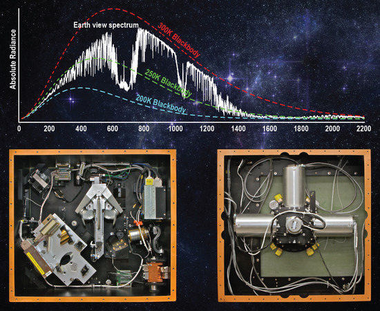
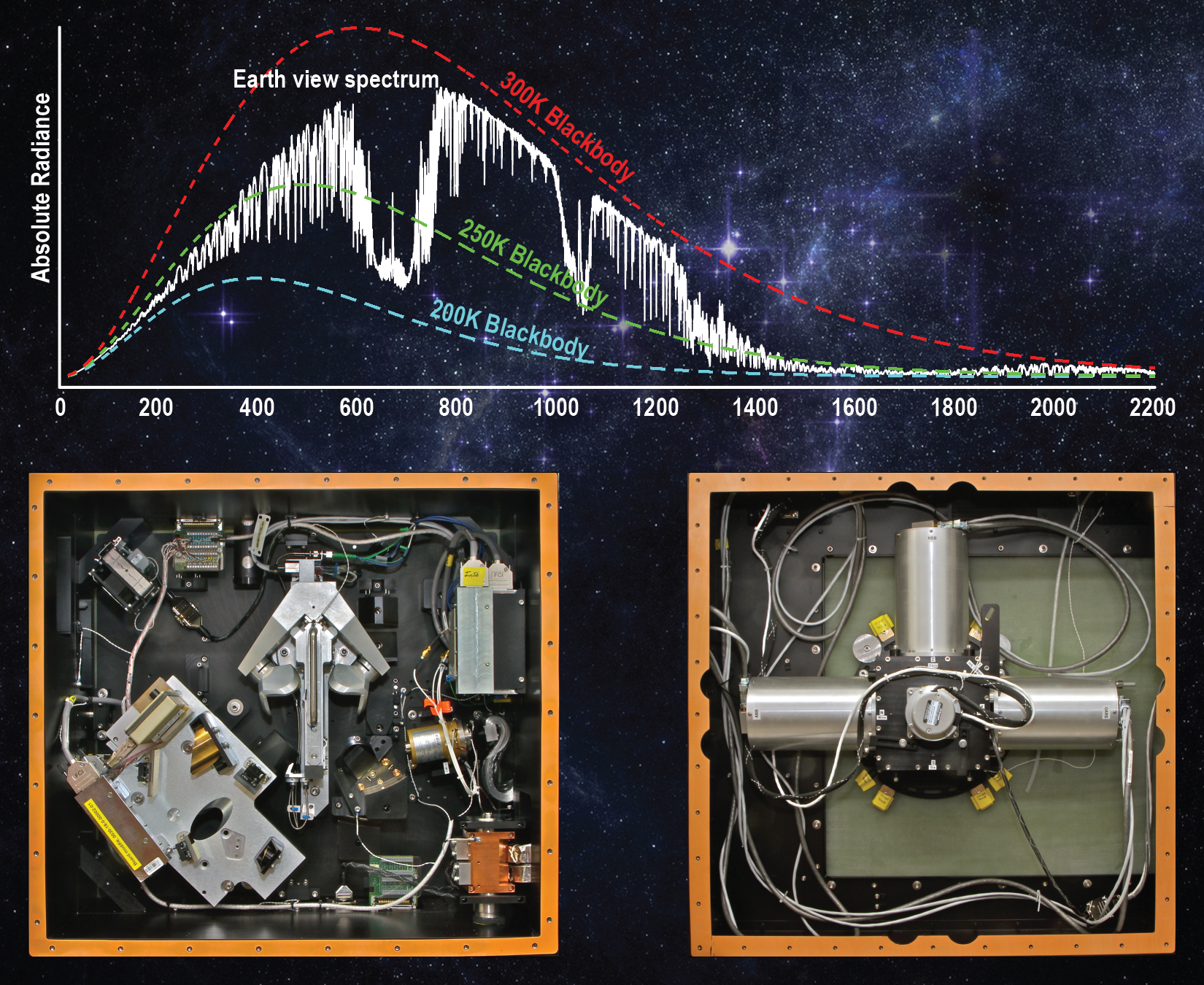
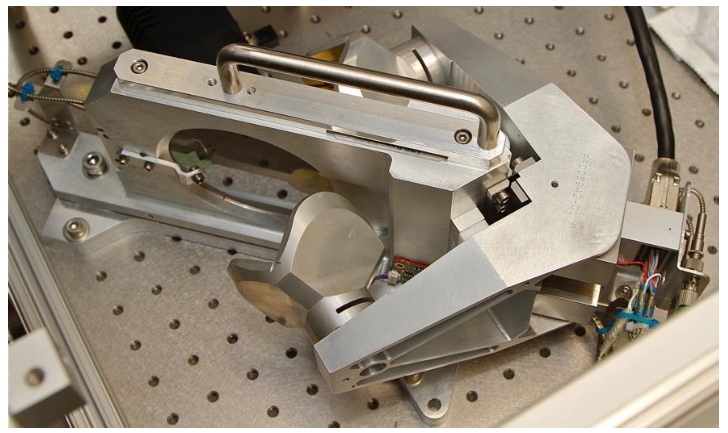
3. The Absolute Radiance Interferometer (ARI)

The Absolute Radiance Interferometer (ARI) consists of a Calibrated Fourier Transform Spectrometer (CFTS), calibrated on-orbit in the traditional way using an ambient onboard blackbody reference and a space view, and an On-orbit Verification and Test System (OVTS) that provides end-to-end calibration verification with direct on-orbit traceability to absolute standards. The OVTS consists of fundamentally new subsystems including the On-orbit Absolute Radiance Standard (OARS) [20,21,22,23], On-orbit Cavity Emissivity Modules (OCEMs) [24,25,26,27,28], and an On-orbit Spectral Response Module (OSRM). The ARI CFTS measures absolute spectrally resolved infrared radiance with a spectral coverage of 200–2000 cm⁻¹ at 0.5 cm⁻¹ spectral sampling (unapodized) and a radiometric measurement accuracy of <0.1 K (k = 3) brightness temperature at scene temperature. Resolving atmospheric spectral lines allows ARI to provide products for climate trending with much higher information content than those from current radiation budget measurements. While the ARI accuracy requirements are demanding, the overall instrument is relatively simple and low-cost, because of the modest requirements on spatial sampling (25–100 km nadir-only footprints spaced at <200 km) and noise performance [3,29]. The minimal spatial sampling and noise requirements derive from the need to perform a great deal of spatial and temporal averaging in deriving climate products that suppress natural variability signals for assessing long-term trends. Also, sampling is limited to nadir-only viewing to suppress potential biases connected with variable view-angle sampling. The CFTS and OVTS are described in detail in Section 4 and Section 5, respectively.

The normal on-orbit operational concept for the ARI is very simple, repeating a series of four spectral samples every 20 s. Three samples are used to collect the primary calibrated Earth-viewing data record; a single nadir view of the Earth is accompanied by views of the onboard calibration blackbody and the primary space view such that the full calibrated measurement cycle is performed frequently. The fourth sample is used to view one of the OVTS sources. For example, views of the OARS are collected over the full range of earth scene brightness temperatures every month. The other scenes that are viewed less frequently include (1) the secondary space view, (2) the OARS with emissivity monitoring sources of the On-orbit Cavity Emissivity Monitor (OCEM) activated, and (3) the On-orbit Spectral Response Monitor (OSRM). More details of the OVTS sequence are presented in Section 5. For efficient data collection, interferograms are recorded for both interferometer sweep directions, and calibration is completed separately for each interferometer mirror sweep direction.

Calibration accuracy and direct traceability to absolute standards are equally important to climate benchmark measurements. Accordingly, it is prudent to adopt the terminology and evaluation of measurement uncertainty recommended by the national and international institutions that govern traceability to the Système international d’unités (SI). The Bureau International des Poids et Mesures (BIPM) ensures worldwide uniformity of measurements and their SI traceability. The BIPM Joint Committee for Guides in Metrology (JCGM) has responsibility for the following two documents: the Guide to the Expression of Uncertainty in Measurement (known as the GUM) [30]; and the International Vocabulary of Metrology—Basic and General Concepts and Associated Terms (known as the VIM) [31]. The vocabulary and uncertainty analysis methods described in this section, and adopted for this effort follow the recommendations presented in the JCGM GUM and VIM, and the US National Institute of Standards and Technology (NIST) guidelines.

The result of a measurement is not ideal, and only an approximation or estimate of the value of the measurand. Thus, the result is complete only when accompanied by a quantitative statement of its uncertainty [32]. The combined standard uncertainty of a measurement result, u_c(y), is taken to represent the estimated standard deviation of the result, and is the positive square root of the estimated variance. The variance is obtained by combining the individual uncertainties and covariances as appropriate:

$$u_c{}^2\left(y\right)={{\displaystyle \sum _{i=1}^N\left(\frac{\partial f}{\partial x_i}\right)}}^2{u}^2(x_i)+{\displaystyle \sum _{i=1}^N{\displaystyle \sum _{\begin{array}{l}j=1\\ j\ne i\end{array}}^N\frac{\partial f}{\partial x_i}\frac{\partial f}{\partial x_j}}}u(x_i,x_j).$$

(1)

In Equation (1), f is the functional relationship between the measurement, y, and the input estimates, x_i, u(x_i) is the standard uncertainty associated with each x_i, u(x_i,x_j) is the estimated covariance associated with x_i and x_j, and the partial derivatives ∂f/∂x_i are often referred to as the sensitivity coefficients. If the individual uncertainties are independent, then u(x_i,x_j) = 0 and Equation (1) reduces to:

$$u_c{}^2\left(y\right)={{\displaystyle \sum _{i=1}^N\left(\frac{\partial f}{\partial x_i}\right)}}^2{u}^2(x_i).$$

(2)

This method is often called the law of propagation of uncertainty and commonly referred to as the “root-sum-of-squares” or “RSS” method of combining uncertainty components estimated as standard deviations. Equation (2) is only valid if the input quantities x_i are not significantly correlated. The combined standard uncertainty u_c is a widely employed measure of uncertainty. However, a measure of uncertainty that defines an interval about the measurement result within which the value of the measurand is confidently believed to lie is often of more practical use. The measure of uncertainty intended to meet this requirement is termed expanded uncertainty, U, and is obtained by multiplying u_c by a coverage factor, k. When the normal distribution applies, k = 2 defines an interval having a level of confidence of approximately 95 percent, and k = 3 defines an interval having a level of confidence greater than 99 percent. Traditionally, outside the field of metrology, the confidence level has been specified by describing expanded uncertainties as 2-σ or 3-σ uncertainties (k = 2 or k = 3 respectively).

4. The Calibrated Fourier Transform Spectrometer (CFTS)

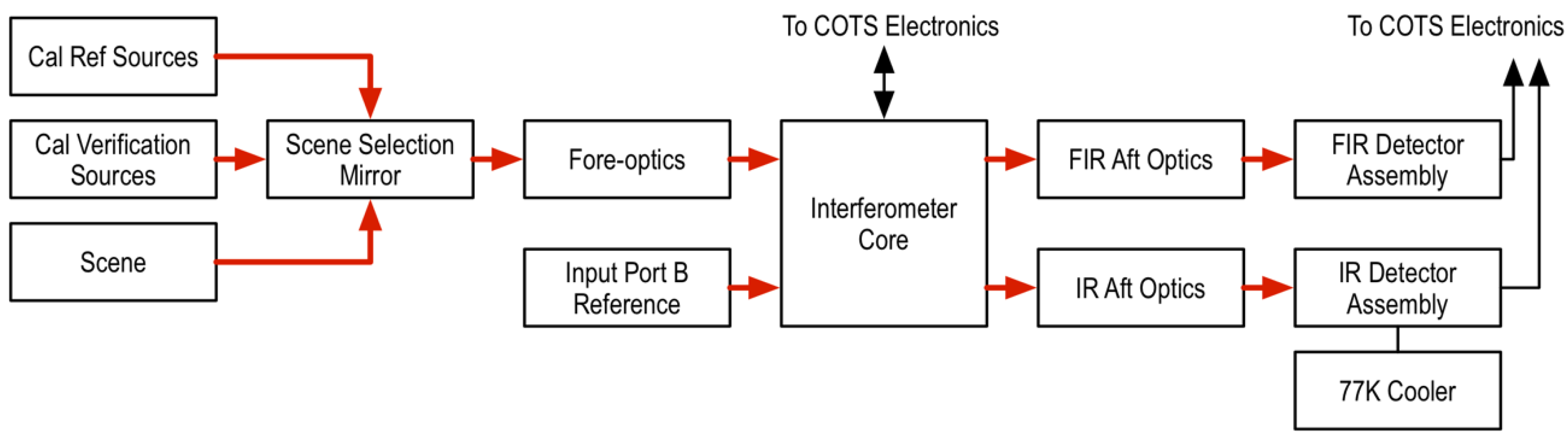
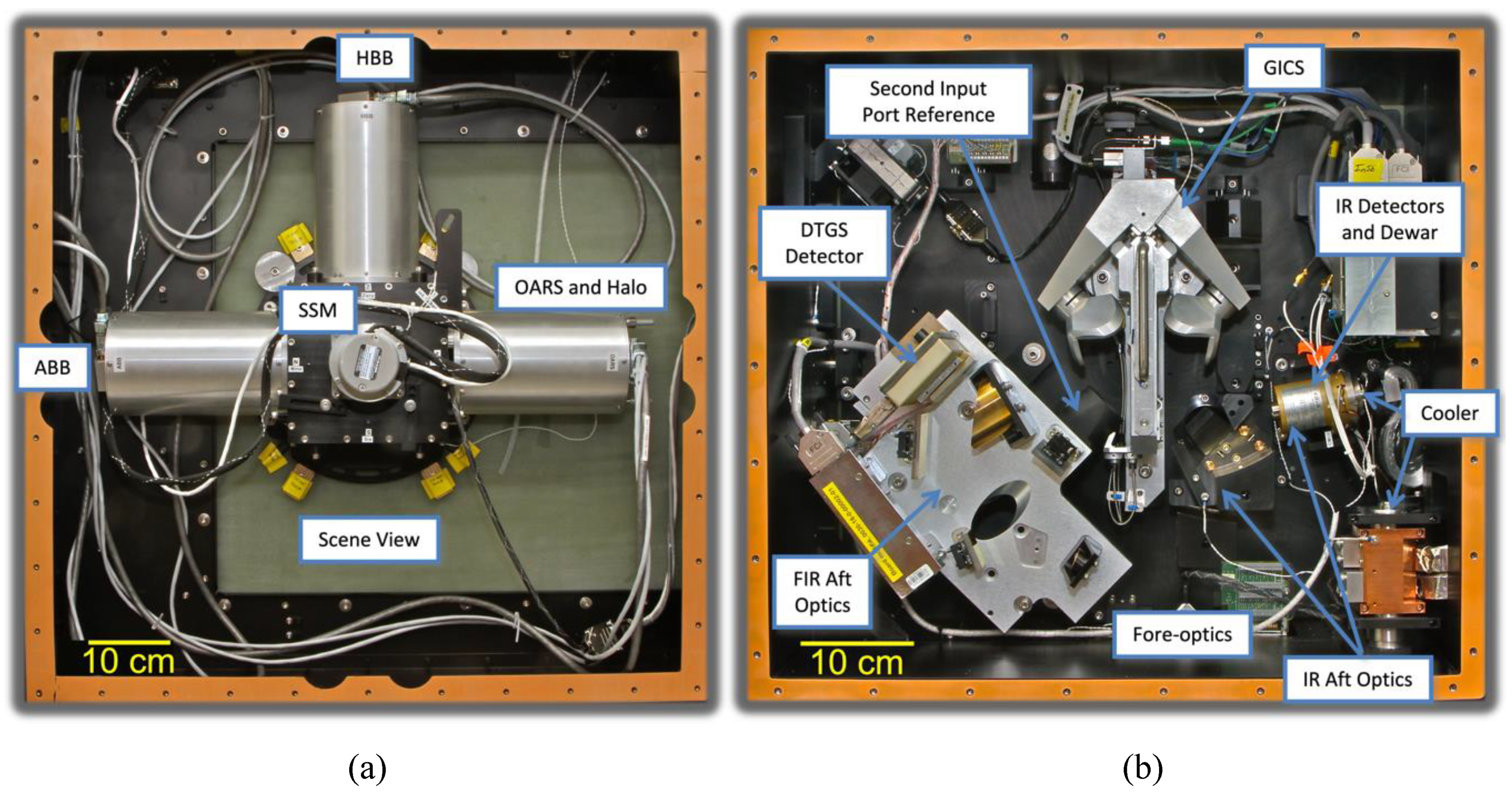
4.1. Design and Overview

A notional block diagram of the Calibrated Fourier Transform Spectrometer is shown in Figure 2. Photos of the completed ARI sensor prototype are provided in Figure 3. The CFTS is comprised of:

• Ultra-high accuracy blackbody calibration reference source(s). During laboratory and vacuum testing two calibration references are required, while a single onboard calibration reference and a deep-space view are used for flight;
• A scene selection mirror assembly;
• A fore-optics telescope designed specifically for high radiometric accuracy;
• A 4-port cube-corner, rocking arm interferometer with a fiber-coupled diode laser-based metrology system;
• Two aft optics assemblies, 1 at each output port of the interferometer;
• A 77 K multiple semi-conductor detector (450–2000 cm⁻¹) and dewar assembly;
• A very small mechanical cooler for the semi-conductor detector and dewar subassembly;
• A DTGS (deuterated triglycine sulfate) pyroelectric detector (200–1400 cm⁻¹) assembly.

The instrument was designed such that detailed performance testing can be conducted on a mature system with a short upgrade path to a spaceflight configuration. For compatibility with the instrument incubator program (IIP) budget and schedule, laboratory-grade and commercial off-the-shelf (COTS) electronics were used.

4.1.1. Key Trade-Studies

Several trade-studies were conducted during the CFTS design phase. Key studies and considerations included interferometer configuration and beamsplitter type, Technological Readiness Level (TRL) and flight heritage, optical throughput, optical stop locations, polarization, detector spectral bands, and signal chain linearity and sensitivity.

The considerations particular to the interferometer core included spectral resolution and range, etendue, beam divergence, size, weight, and power, and vibration and temperature sensitivity. Cube-corner retroreflectors were selected over plane mirrors for the interferometer, based on current cube-corner manufacturing and assembly capabilities, the reduced modulation sensitivity to shear compared to tilt, and the required maximum optical path difference (MOPD) for the ARI system. Since a four-port interferometer configuration is immune to the double pass problem, a concern for the broadband coverage requirements, a four-port design was chosen. Finally, several beamsplitter options were considered. Pellicle and wire grids were considered as beamsplitter candidates. However, they are extremely delicate, vibration-sensitive, and provide limited shortwave IR coverage and due to these concerns, it was decided that pellicle and wire grids were not a feasible option. Beamsplitter materials identified as suitable for the required spectral coverage include Cesium Iodide, Silicon, and chemical vapor deposition (CVD) diamond. Silicon and CVD diamond provide spectral coverage well beyond the longwave requirement (200 cm⁻¹) for the climate benchmark measurement. While Silicon has outstanding efficiency well below 100 cm⁻¹, it exhibits strong phonon absorption at 618 cm⁻¹. Phonon absorption is dependent on material thickness and can be minimized by making the silicon wafer very thin. In CVD diamond, intrinsic absorption limits its efficiency at shorter wavelengths. Given these characteristics, a single plate uncoated and uncompensated beamsplitter configuration would be the best option for both Silicon and CVD diamond for our required spectral coverage. The primary concern with this configuration is the associated extensive optical channeling. Channeling amplitude may be controlled through increasing beam divergence and optical element thickness, and the channeling frequency is also a function of element thickness. However, beam divergence and beamsplitter thickness are also subject to other design constraints. The stability of the fringing depends on temperature stability, and the material’s refractive index temperature dependence and thermal expansion coefficient. Accordingly, additional constraints are placed on the thermal stability of the beamsplitter temperature during the calibration cycle if the effect is to be made negligible after calibration. Lastly, and perhaps most importantly for this prototype demonstration, Silicon and CVD diamond beamsplitters did not have significant flight heritage and would require additional testing and technology development beyond the scope of the project. With these considerations in mind, CVD diamond and Silicon were not chosen for the prototype. Cesium Iodide, while highly hygroscopic and requiring careful handling, satisfies the spectral coverage requirements and has the necessary flight heritage and was selected as the most suitable beamsplitter material for the ARI demonstration. To minimize losses and maximize performance, a single substrate, self-compensated configuration was chosen. This design provides precise compensation of optical path difference (OPD) dispersion and a highly symmetric interferogram.

4.1.2. The Interferometer Modulator

The challenge in the infrared FTS sensor development for a climate benchmark mission such as CLARREO is to achieve ultra-high accuracy (0.1 K, ≥99% confidence) with a design that can be flight-qualified, has long design life, and is reasonably small and affordable. The CFTS is built around the ABB (Quebec, Canada) provided Generic Interferometer for Climate Studies (GICS), which is based directly on the ABB Generic Flight Interferometer (GFI). ABB has participated in many mission definitions involving FTS and the strong similarities in the requirements at the level of the interferometer module for these missions caused ABB to pursue developing a generic flight architecture, the Generic Flight Interferometer (GFI). The GFI includes an Opto-Mechanical Assembly (OMA) that consists of an interferometer modulator equipped with a metrology assembly. The OMA is entirely free of electronic components apart from the interferometer scanning actuator. A 6U control card that conveys the functionality of metrology detection, laser source, actuator drive, servo control, housekeeping, telemetry, and command/data handling complements this Opto-Mechanical Assembly (OMA). The OMA architecture draws its heritage from a commercial instrument (Bomem MB Series) that dates back to the mid-1980s. This instrument is known for its exquisite response stability and is used in production plants around the world to provide critical concentration measurement as control feedback for industrial fabrication processes. The ACE-SCISAT FTS was the first to implement a space design based on this architecture. Launched in 2003, ACE continues to operate today (2020), well beyond its design lifetime requirement of 2 years. More recently the TANSO-FTS onboard IBUKI (GOSAT) launched in 2009 and TANSO FTS-2 on GOSAT-2 launched in 2018 by JAXA were also based on an evolution of the ACE-FTS and MB Series design. The GFI and GICS thus represent the third generation of flight interferometers and includes some of the latest technology developed for commercial applications. A photo of the GICS is provided in Figure 4.

To meet the UW-SSEC CFTS requirements, only small adaptations of the GFI architecture were required. The resulting interferometer core is the ABB Generic Interferometer for Climate Studies. The key differences from the GFI are

• The beam splitter substrate and coatings have been replaced with materials that maximize efficiency over the 3–50 μm range (CsI beam splitter, modified production coating);
• Mounting of the beam splitter has been optimized for CsI material properties;
• A self-compensated beam splitter design is used instead of a substrate and compensator design;
• GICS utilizes a 4-port configuration while GFI uses a 2-port configuration;
• Laser metrology components have been relocated for compatibility with 4-port operation;
• Replicated monolithic cube-corners are used in the GICS;
• Due to cost considerations, the GFI flight electronics were replaced with modified commercial electronics and software for the IIP demonstration.

The GICS is a vacuum compatible interferometer. The IIP demonstration unit has a mass of <7 kg (Opto- Mechanical Assembly), and the power requirements for the flight design are 18 W average, 23 W peak. Again, for cost considerations modified COTS electronics are used for the ARI demonstration. It is assumed that a new coating recipe with optimized FIR performance would be used for the flight unit, rather than the modified production unit coating used in the prototype.

4.1.3. Fore and Aft Optics

The fore-optics and FIR aft-optics consist of all reflective elements. The IR aft-optics assembly consists of two reflective elements, combined with in-dewar 77 K refractive optics. Each reflective element is diamond point turned aluminum, plated with uncoated Epner Gold. The use of uncoated gold minimizes polarization while maintaining high transmission. The optical design goals included:

• Optimization of interferometer throughput;
• Maximal stray light control;
• Minimization of instrument mass and volume;
• Optimization of the heated halo geometrical fill factor;
• Compatibility with a 1” aperture Blackbody;
• Capability for tuning of polarization sensitivity “null” locations with respect to the position of the calibration reference bodies, OARS, and scene views.

These goals, combined with other instrument requirements, resulted in a fore-optics design that provides an afocal magnification of 2.3, accommodates well-defined field and aperture stops, and relays the aperture stop to pupils at the interferometer cube-corner and the halo entrance aperture.

In the ARI, the polarization induced calibration bias depends on the scene select mirror rotation angle. Models predicted that the dependence is sinusoidal with four equally spaced zero-crossings for 360° of rotation of the scene select mirror. The instrument was designed with the calibration, calibration verification, and scene viewports at 90° spacing in the scene selection mirror rotation angle. Additionally, the ARI instrument design provides the ability to rotate the calibration and verification module with respect to the sensor such that the position of the viewports can be rotated to finely tune the viewport placement with respect to the zeroes of the polarization induced calibration bias. This design feature also provides the capability to confirm the orientation of the sensor’s polarization sensitivity via measurement. Tests were conducted to determine the polarization sensitivity of the instrument and confirm the model predicted position of the polarization induced calibration bias zero-crossings. See Taylor [33] for further details of the polarization model and test results.

Due to schedule and budget considerations, the FIR aft-optics module for the prototype is based on a commercially available system modified to include a field and aperture stop such that the sensor may be operated without the fore-optics in the system, which was desirable for early testing. The aft-optics stop sizes are adjustable and removable, such that they can be adjusted so that they are not the limiting stops when the fore-optics are installed in the system and to provide flexibility during testing.

4.1.4. Detector Modules

Due to the high radiometric accuracy requirements, and relatively undemanding noise requirements, it is possible and important to emphasize linearity rather than sensitivity for detector screening and signal chain design for the flight instrument; however, due to cost and schedule considerations associated with the demonstration effort, readily available commercial options were selected for the signal chain electronics and the FIR deuterated triglycine sulfate (DTGS) pyroelectric detector, and an existing UW-SSEC detector and dewar assembly was used. The existing UW-SSEC detector dewar assembly houses a shortwave Indium Antimonide (InSb), and three photoconductive (PC) Mercury-Cadmium-Telluride (HgCdTe or MCT) detectors providing spectral coverage from 420–3300 cm⁻¹ (extended longwave MCT: 400–1600 cm⁻¹, longwave MCT: 550–1700 cm⁻¹, midwave MCT: 800–1820 cm⁻¹, shortwave InSb: 1820–3300 cm⁻¹). For the ARI demonstration, the longwave MCT and FIR DTGS detector channels were used.

The photovoltaic (PV) InSb detector exhibits an extremely linear response, and the test and analysis of the DTGS detector indicate its nonlinearity, including signal chain electronics, to be less than 0.01%. The nonlinear response of photoconductive (PC) MCT detectors is well established, with documented nonlinear behavior ranging from a few percent to more than 20% deviation from linearity at maximum flux intensities. The nonlinear response of the MCT detectors used in the ARI prototype demonstration is not insignificant (on the order of a few percent), and a nonlinearity correction needed to be applied to the MCT detector signal response prior to radiometric calibration for the prototype measurements. The nonlinearity correction used for the ARI prototype MCT detectors is an algorithmic approach, built on the nonlinearity correction method developed at the UW-SSEC. The UW-SSEC nonlinearity correction algorithm is based directly on photoconductive (PC) HgCdTe detector theory [34] and has been successfully applied to the AERI (Atmospheric Emitted Radiance Interferometer) [9,35,36], S-HIS (Scanning High-resolution Interferometer Sounder) [11], NAST-I (NPOESS Airborne Sounder Testbed–Interferometer) [37], and CrIS (Cross-track Infrared Sounder) [18,38,39] sensors. While the CrIS detectors are photovoltaic (PV) HgCdTe, the CrIS instrument demonstrated a second-order nonlinear detector response. The nonlinearity correction applies to any nonlinear response that can be expressed as a polynomial expansion, regardless of the physical principles that result in the nonlinear response. Details of the nonlinearity assessment and correction for the ARI longwave MCT detector are provided by Taylor [33].

It is also notable that the 4-port configuration of the interferometer allows a direct comparison between the two output ports of detector response in overlapping spectral regions. The linear DTGS detector and nonlinear MCT detectors, located at opposite output ports, have simultaneous and overlapping spectral coverage from 450 cm⁻¹ to 1800 cm⁻¹. This is useful for confirming the effectiveness of the nonlinearity correction for the ARI prototype MCT detectors.

4.2. Radiometric Calibration and Uncertainty

The complex calibration method is used for the calibration of the ARI. Complex calibration is an efficient method developed to correct the amplitude and phase of the measured spectrum [6]. This approach requires two distinct calibration references. The basic calibration expression for the complex calibration method is:

$$L_S\left({\nu }_k\right)=\left(L_H\left({\nu }_k\right)-L_C\left({\nu }_k\right)\right)\mathrm{Re}\left\{\frac{{\mathbb{S}}_S\left({\nu }_k\right)-{\mathbb{S}}_C\left({\nu }_k\right)}{{\mathbb{S}}_H\left({\nu }_k\right)-{\mathbb{S}}_C\left({\nu }_k\right)}\right\}+L_C\left({\nu }_k\right).$$

(3)

In Equation (3), L_S(ν_k) is the calibrated radiance at wavenumber sampling interval ν_k; S_S(ν_k), S_C(ν_k), and S_H(ν_k) are the complex measured spectra for the scene, cold reference, and hot reference views respectively; and L_C(ν_k) and L_H(ν_k) are the calculated radiances for the respective cold and hot reference views. Radiances are expressed in units of mW/(m²·sr·cm⁻¹), and the wavenumber scale is specified in units of cm⁻¹. The calculated radiance from a non-ideal blackbody cavity is the sum of the emitted and reflected radiance from the cavity:

$$L\left({\nu }_k\right)=e\left({\nu }_k\right)B({\nu }_k,T)+\left(1-e\left({\nu }_k\right)\right)B({\nu }_k,T_R),$$

(4)

where e(ν_k) is the effective emissivity of the blackbody, B(ν_k,T) is the Planck radiance for an ideal blackbody of temperature T, and B(ν_k,T_R) is the Planck radiance of the background, of mean temperature T_R, that is reflected from the cavity, assuming that the background contribution can be approximated by a Lambertian emitter at temperature T_R. The radiances can be converted to equivalent brightness temperatures via inversion of Planck’s Law.

Interferograms are recorded for both interferometer sweep directions. The spectra for each sweep direction are calibrated separately, since the phase behavior of the measured spectra can be dependent on sweep direction. If the reference spectra are collected with sufficient frequency such that the change in instrument emission between reference views is small and the measured spectra and calculated radiances for the reference views may be accurately interpolated to the time of the scene measurement, then any complex offset or phase associated with the warm instrument emission is canceled in the ratio of complex difference spectra contained in Equation (3).

A differential error analysis of the calibration equation was used to guide the instrument development of the ARI. This approach was key to focusing the instrument design on minimizing radiometric uncertainty, the driving requirement for CLARREO-type climate benchmarking. The analysis utilized the same methodology that was used as the basis for the radiometric uncertainty estimates, shown in Figure 1 (and explained earlier in that context) and discussed in further detail in this section. This methodology is consistent with the accepted metrology approach to uncertainty analysis. The accuracy of the reference blackbodies was then chosen to ensure that the instrument measurements that enter into the calibration equation are adequate to meet the overall calibration requirements. The ARI reference blackbodies are based on the UW-SSEC Geostationary Imaging FTS (GIFTS) blackbody design [40,41]. Minor design modifications were made for the OARS, along with the addition of multiple miniature phase-change cells. The effective temperature uncertainty for the ARI reference blackbodies and OARS, are summarized in

Table 2. ARI calibration source and OARS temperature uncertainty budget. All specified uncertainties correspond to a k = 3 coverage factor. Note that a temperature uncertainty of 0.045 K for the calibration reference blackbodies and the OARS is used in the ARI radiometric uncertainty analysis for all environments. Refer to Siwek et al. [42] for further details on the thermistor stability.

	Temperature Uncertainty [K] (3-σ)
Source of Error	Laboratory OARS & ARI Cal Sources	On-Orbit ARI Cal Source	On-Orbit OARS
Thermistor Temperature Calibration Uncertainty
Temperature Probe Standard or Melt Plateau Determination (for On-Orbit)	0.005	0.005	0.010
Transfer of T Probe or Melt Cell to Thermistor uncertainty (gradients during cal.)	0.010	0.010	0.002
Thermistor Calibration Equation Interpolation Error Between Cal. Pts.	0.002	0.002	0.016
Cavity Temperature Uniformity Uncertainty
Cavity to Thermistor Gradient Uncertainty (1/2 of max expected gradient)	0.015	0.015	0.015
Thermistor Wire Heat Leak Temperature Bias Uncertainty *	0.020	0.008	0.020
Paint Gradient (due to radiative coupling to surrounding temperatures)	0.018	0.015	0.018
Stability Between Calibrations
Blackbody Thermistor (From [42] with factor applied for configuration differences)	0.005	0.010	0.005
Blackbody Thermistor Readout Electronics	0.001	0.015	0.005
Effective Radiometric Temperature (Teff) Weighting Factor Uncertainty
Monte Carlo Ray Trace Model Uncertainty in Determining Teff	0.030	0.025	0.025
(radiometric error that accounts for non-isothermal cavity temperature) (On-Orbit cases improved due to additional modelling)
RSS Combination	0.045	0.040	0.045

* Due to conductive coupling of leads to a temperature different that the cavity.

.

The uncertainty associated with the calibrated radiance may be estimated by calculating the combined uncertainty for L_S(ν_k) (Equation (3)). There is no expected first-order correlation for the input quantities in Equation (3), and it is valid to use Equation (2) (RSS method) for estimation of the combined uncertainty:

$$\begin{array}{cc}\hfill u_{L_S}{}^2=& {\left(\frac{\partial L_S}{\partial T_H}\right)}^2{u}^2\left(T_H\right)+{\left(\frac{\partial L_S}{\partial e_H}\right)}^2{u}^2\left(e_H\right)+{\left(\frac{\partial L_S}{\partial T_{R,H}}\right)}^2{u}^2\left(T_{R,H}\right)\hfill \\ & +{\left(\frac{\partial L_S}{\partial T_C}\right)}^2{u}^2\left(T_C\right)+{\left(\frac{\partial L_S}{\partial e_C}\right)}^2{u}^2\left(e_C\right)+{\left(\frac{\partial L_S}{\partial T_{R,C}}\right)}^2{u}^2\left(T_{R,C}\right)\hfill \\ & +{\left(\frac{\partial L_S}{\partial X}\right)}^2{u}^2\left(X\right).\hfill \end{array}$$

(5)

In Equation (5) T_H and T_C are the temperatures of the hot and cold calibration reference targets, with respective uncertainties u(T_H) and u(T_C); T_R,H, T_R,C are the mean temperature of the background radiance that is reflected from the hot and cold reference targets, with respective uncertainties u(T_R,H) and u(T_R,C); e_H and e_C are the effective emissivities of the hot and cold blackbodies, with uncertainties u(e_H) and u(e_C); and X represents the measured spectra term:

$$X=\mathrm{Re}\left\{\frac{{\mathbb{S}}_S\left({\nu }_k\right)-{\mathbb{S}}_C\left({\nu }_k\right)}{{\mathbb{S}}_H\left({\nu }_k\right)-{\mathbb{S}}_C\left({\nu }_k\right)}\right\}.$$

(6)

Assessment of the combined uncertainty u(X) of the measured spectra is completed via models and perturbation analysis. For a well-designed FTS sensor, it is expected that the dominant source of uncertainty associated with the measured spectra will be signal chain nonlinearity and polarization. This expectation is based on past experience with design, analysis, and testing of the AERI [9,35,43,44,45], S-HIS [46,47,48,49], and GIFTS [40,50] instruments, and testing and analysis of the CrIS [18,51,52] instrument. As noted previously, due to the high radiometric accuracy requirements, and relatively undemanding noise 4 requirements, it is recommended that linearity rather than sensitivity is prioritized for detector selection and signal chain design for the flight instrument. Based on the radiometric uncertainty analysis and the required calibration accuracy, the residual nonlinearity, expressed as a percentage error, should be limited to less than 0.03%. While polarization sensitivity induced calibration error can be a significant contributor to measurement uncertainty for infrared instruments, the ARI optical design mitigates first and second-order polarization induced calibration errors.

Accordingly, the primary radiometric uncertainty contributions are associated with the calibration reference temperature and emissivity uncertainties. Signal chain nonlinearity and polarization induced calibration biases are expected to be insignificant in comparison and are not included in the predicted calibration and calibration validation uncertainty analysis in Section 4.3. Furthermore, based on the radiometric uncertainty analysis completed via the perturbation of the complex calibration equation, a limit can be established for the radiometric uncertainty contribution associated with less significant contributors, such that the 0.1 K on-orbit requirement can still be met with sufficient margin. Pre-launch characterization and testing of the instrument must verify that the instrument is performing within expected radiometric uncertainty.

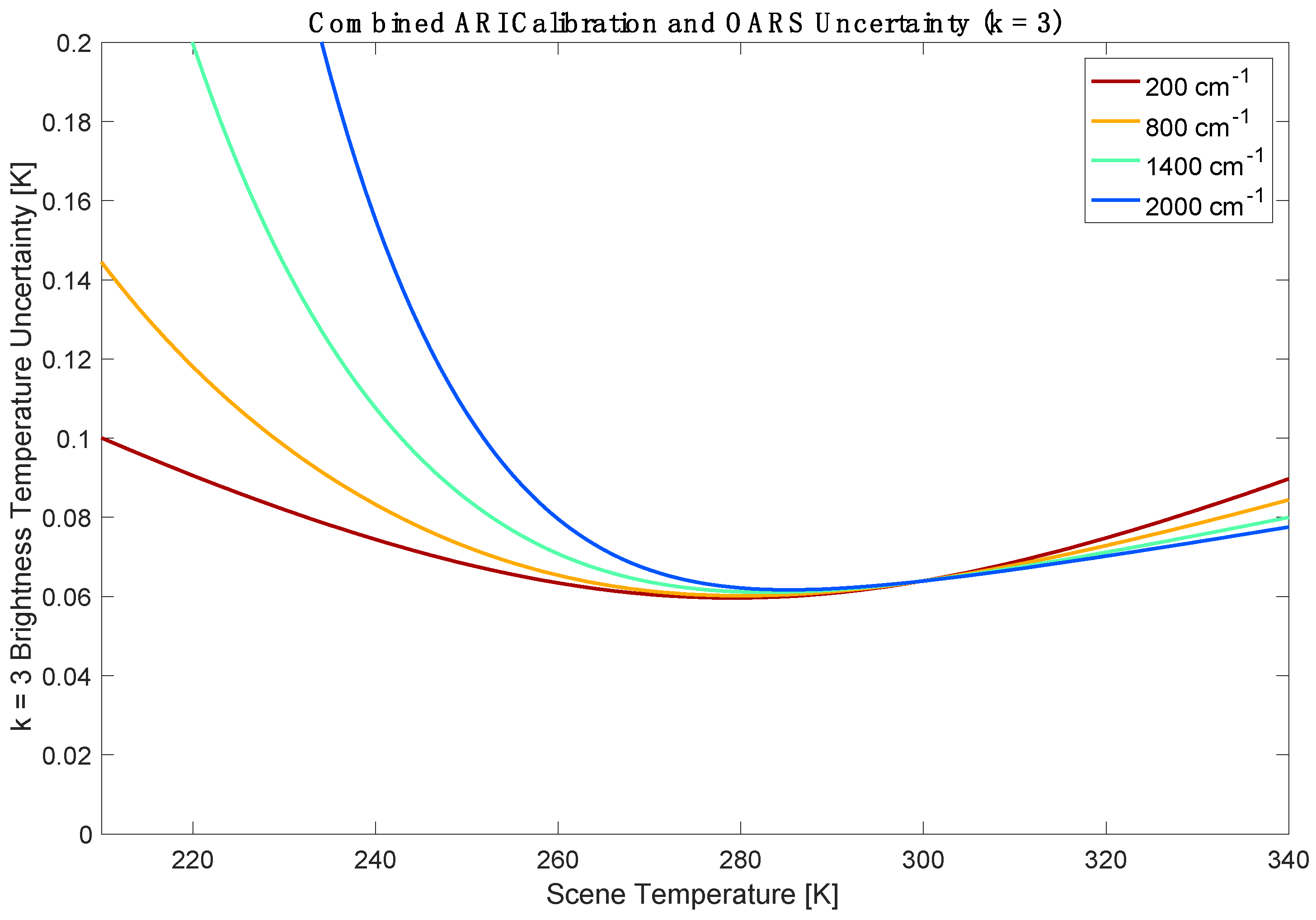
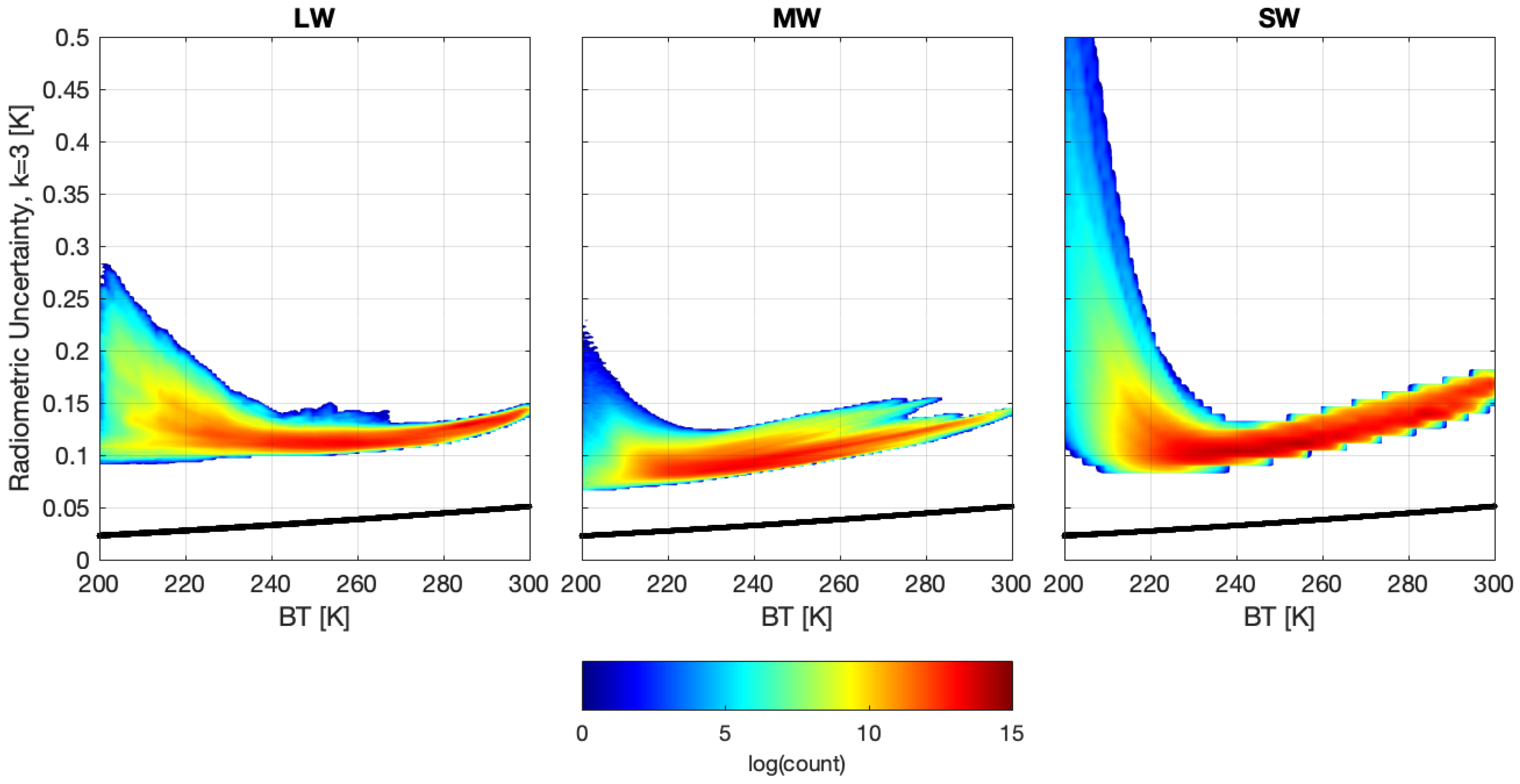
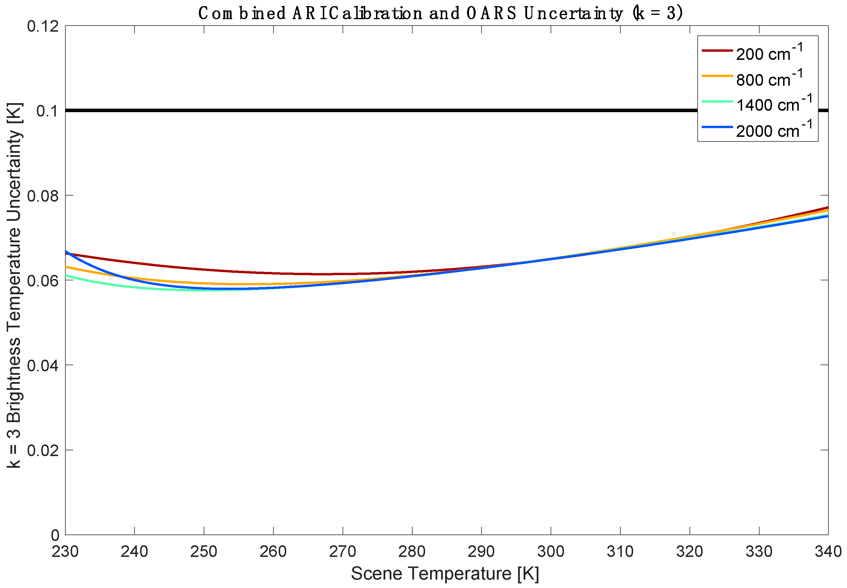
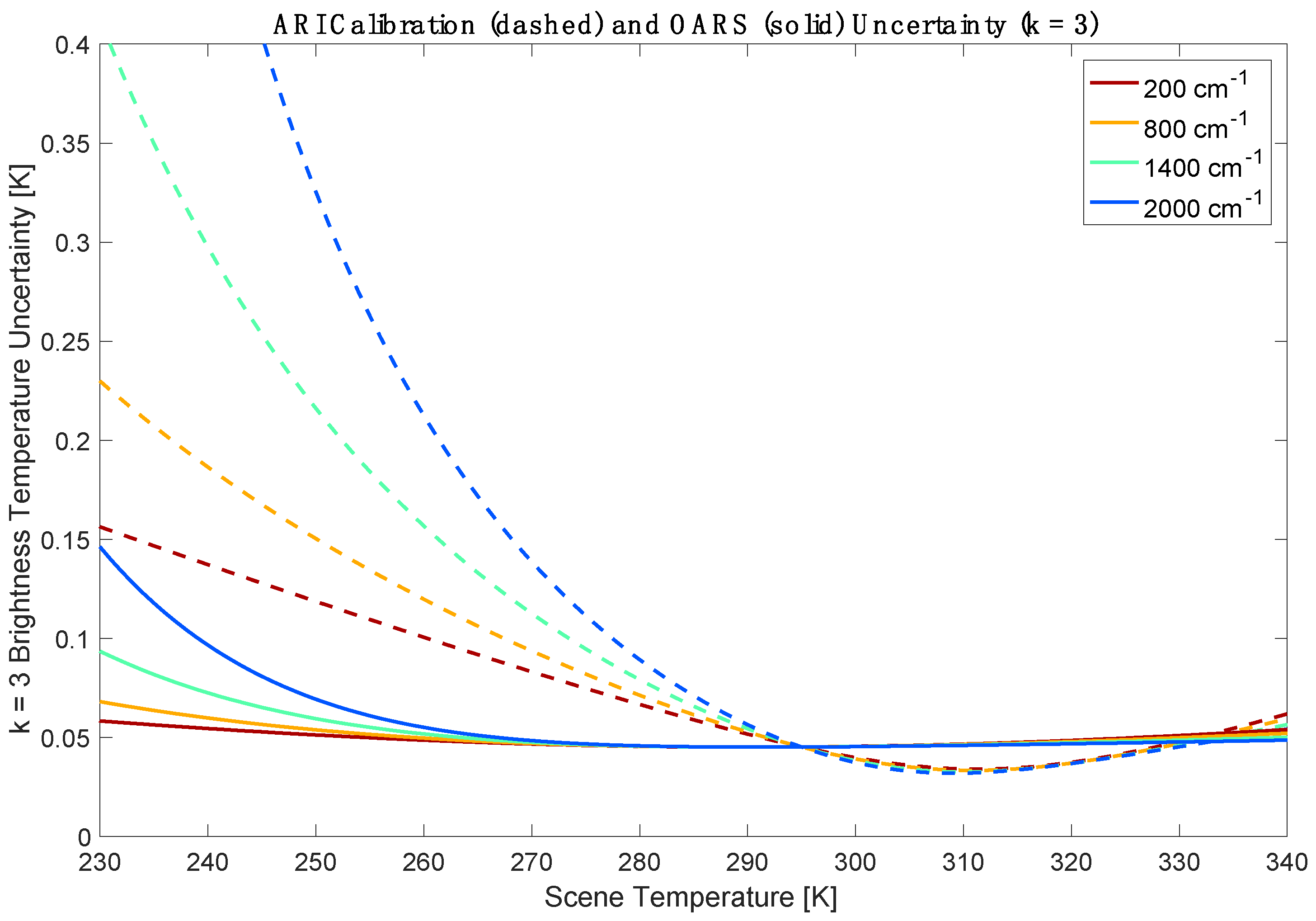
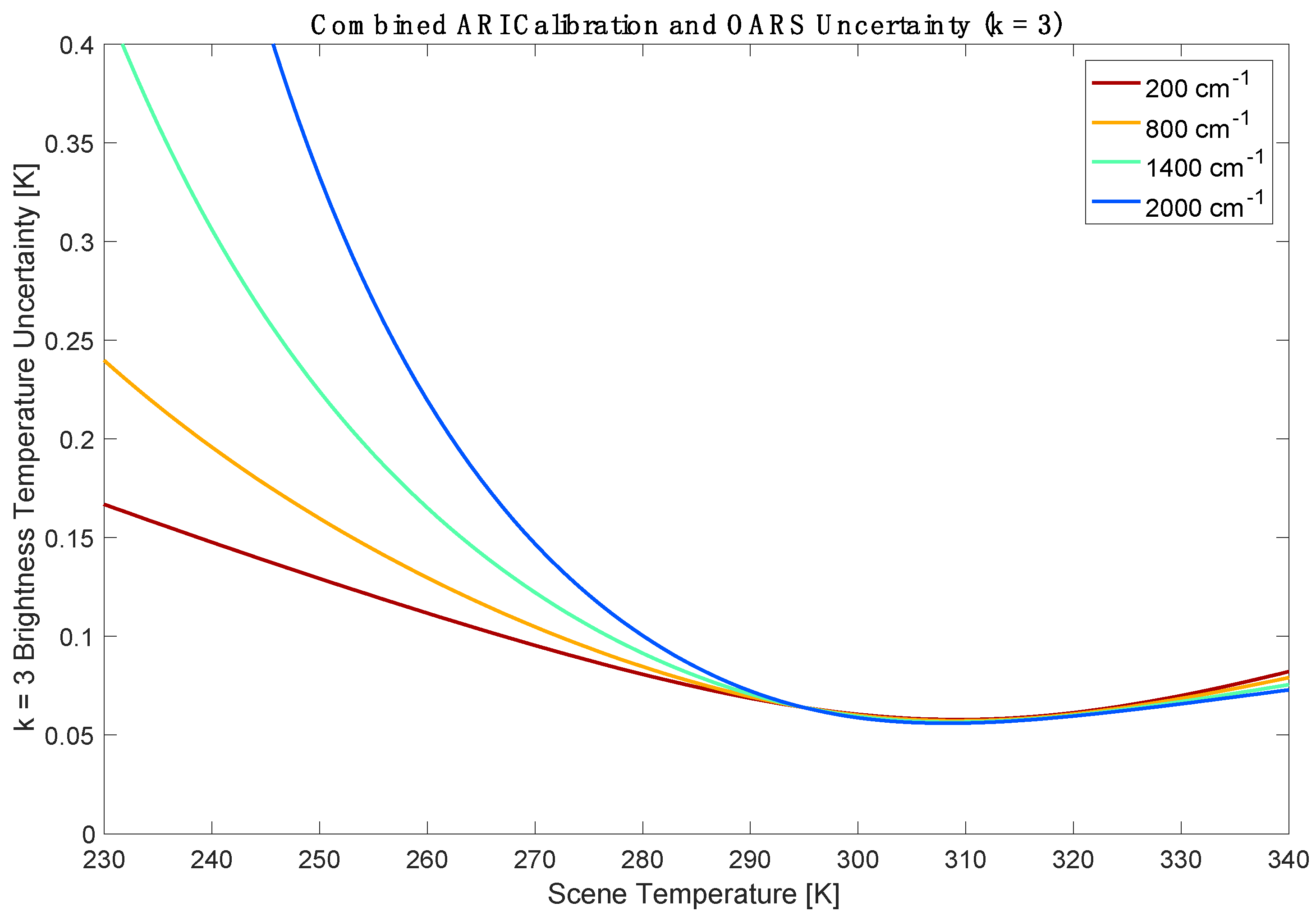
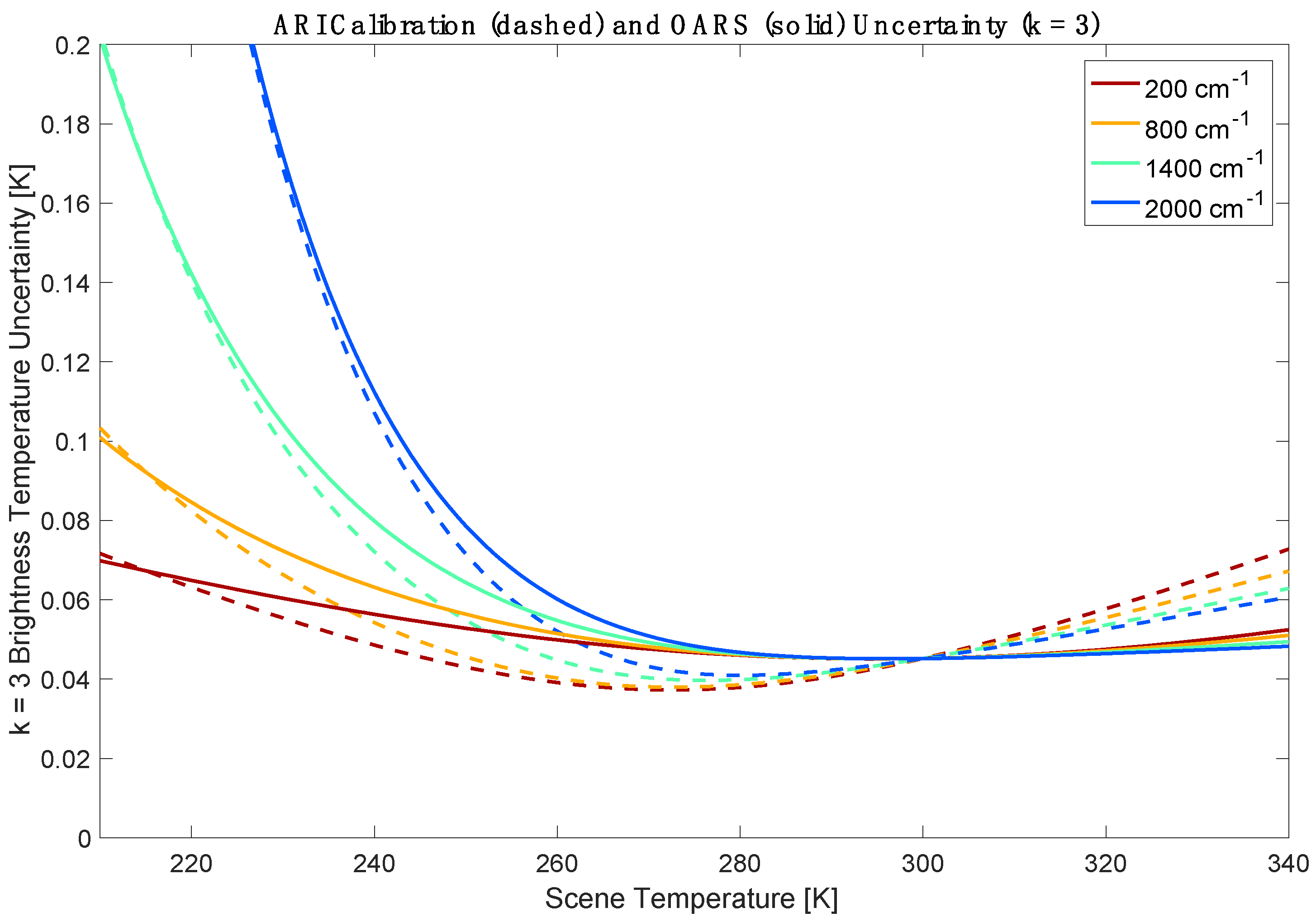
4.3. Predicted Uncertainty

The primary end-to-end radiometric calibration verification process is conducted using the OARS as the SI-traceable reference source. The OARS is operated over a wide range of temperatures for radiometric calibration validation of the CFTS. The resultant measured calibrated brightness temperatures are compared to the predicted brightness temperatures.

The radiance bias ΔL(ν) may be expressed as the difference between the predicted OARS radiance $L_{OARS}\left({\nu }_k\right)$ and the measured calibrated radiance $L_S\left({\nu }_k\right)$:

$$\Delta L\left({\nu }_k\right)=L_{OARS}\left({\nu }_k\right)-L_S\left({\nu }_k\right).$$

(7)

Since we cannot exactly know the OARS true radiance, the uncertainty in the verification of the calibrated radiance includes a contribution from the uncertainty in the determination of the predicted OARS radiance in addition to the uncertainty in the measured radiance:

$$\begin{array}{ll}{u}^2\left(\Delta L\right)& ={\left(\frac{\partial \left(\Delta L\right)}{\partial L_{OARS}}\right)}^2{u}^2\left(L_{OARS}\right)+{\left(\frac{\partial \left(\Delta L\right)}{\partial L_S}\right)}^2{u}^2\left(L_S\right)\\ & =u^2\left(L_{OARS}\right)+u^2\left(L_S\right).\end{array}$$

(8)

Note that in Equation (8), the total uncertainty of the measured calibrated radiance and predicted radiance is given by the root-sum-of-squares since the calibrated measurement and predicted OARS radiance are independent for uncertainty assessment (see Section 3, Equation (2)).

The predicted OARS radiance is calculated using Equation (4) and the radiometric uncertainty associated with the On-orbit Absolute Radiance Standard (OARS), $u_{L_{OARS}}$, is given by:

$$u_{L_{OARS}}{}^2={\left(\frac{\partial L_{OARS}}{\partial T_{OARS}}\right)}^2{u}^2\left(T_{OARS}\right)+{\left(\frac{\partial L_{OARS}}{\partial e_{OARS}}\right)}^2{u}^2\left(e_{OARS}\right)+{\left(\frac{\partial L_{OARS}}{\partial T_{R,OARS}}\right)}^2{u}^2\left(T_{R,OARS}\right).$$

(9)

In Equation (9) $T_{OARS}$ is the temperature of the OARS with uncertainty $u\left(T_{OARS}\right)$, $T_{R,OARS}$ is the mean temperature of the background radiance that is reflected from the OARS cavity with uncertainty $u\left(T_{R,OARS}\right)$, and $e_{OARS}$ is the effective emissivity of the OARS with uncertainty $u\left(e_{OARS}\right)$.

The predicted calibration and calibration validation uncertainty for the on-obit, laboratory, and vacuum calibration configurations and thermal environments are provided in the following sections (Section 4.3.1, Section 4.3.2 and Section 4.3.3 respectively). The temperatures, emissivities, and associated uncertainties for each environment are tabulated, and figures illustrating the calibration, calibration validation, and combined uncertainty are provided. The radiometric uncertainty is expressed as equivalent brightness temperature uncertainty at scene brightness temperature and plotted versus scene brightness temperature at optical frequencies of 200, 800, 1400, and 2000 cm⁻¹. The phrase “brightness temperature uncertainty at scene brightness temperature” emphasizes that this is a specification of true brightness temperature uncertainty. It is common in the field to convert small radiance uncertainties into brightness temperature uncertainties by dividing by the derivative of the Planck function with respect to temperature evaluated at a fixed reference temperature such as 280 K or 300 K. For cold temperatures, such a specification is significantly less demanding than evaluating the Planck function derivative at the scene temperature, which is equivalent to a true brightness temperature uncertainty. Perturbation analysis of the equations for describing the complex calibration method, Equation (3), and the predicted radiance from a non-ideal blackbody, Equation (4), is used to determine the individual uncertainty contributions. The individual radiometric uncertainties are converted to equivalent blackbody brightness temperature, via inversion of Planck’s law. Since there is no expected first-order correlation for the input quantities, the individual uncertainty contributions are combined via the RSS method.

4.3.1. Predicted Uncertainty: On-orbit

Figure 5 shows the total radiometric calibration uncertainty estimate and the validation uncertainty, on-orbit, converted to equivalent brightness temperature. The calibration reference sources on-orbit are a space view target (ST) and the internal calibration target (ICT), which is near instrument (ambient) temperature. Uncertainty estimates are tabulated in

Table 3. Uncertainty estimates used in the radiometric uncertainty analysis for the on-orbit configuration. All specified uncertainties correspond to a k = 3 coverage factor. The temperature uncertainty for the OARS is explained in Section 5. For the flight sensor, it has been assumed that the OARS emissivity and associated uncertainty are determined from laboratory testing with a very high emissivity source. (* e_OARS = 0.999 ± 0.0006 (200 cm⁻¹), ±0.0004 (800 cm⁻¹), ±0.0002 (1400 cm⁻¹), ±0.0001 (2000 cm⁻¹).

Temperatures			Associated Uncertainty
Cold Cal Ref (Space Target)	$T_C$	2.7 K	$u(T_C)$	0 K
Hot Cal Ref (Internal Cal Target)	$T_H$	295 K	$u(T_H)$	0.045 K
Verification Target (OARS)	$T_{OARS}$	230–320 K	$u(T_{OARS})$	0.045 K
Reflected Radiance, Cold Cal Ref	$T_{R,C}$	290 K	$u(T_{R,C})$	0 K
Reflected Radiance, Hot Cal Ref	$T_{R,H}$	290 K	$u(T_{R,H})$	4 K
Reflected Radiance, Verification Target	$T_{R,OARS}$	290 K	$u(T_{R,OARS})$	4 K
Emissivities
Cold Cal Ref (Space Target)	$e_C$	1	$u(e_C)$	0
Hot Cal Ref (Internal Cal Target)	$e_H$	0.999	$u(e_H)$	0.0006
Verification Target (OARS)	$e_{OARS}$	0.999	$u(e_{OARS})$	0.0006 *

. The combined calibration and calibration verification uncertainty is shown in Figure 6. The on-orbit temperatures and uncertainty estimates are based on past experience with the testing and analysis of flight sensors and thermal modeling of the flight environment.

4.3.2. Predicted Uncertainty: Laboratory Testing

For cost compatibility with the scope of the NASA Instrument Incubator Program funding for the ARI prototype development and demonstration, testing during the IIP phase was conducted in a laboratory environment, with ambient temperatures and pressure for all laboratory tests. During the IIP laboratory testing, an ambient calibration blackbody and hot calibration blackbody were used as calibration reference sources. The radiometric uncertainty analysis for this configuration and environment is included herein for completeness, and to provide perspective for the dependence of the radiometric uncertainty on the calibration reference temperature. The challenges associated with this calibration reference configuration and environment include:

• Increased uncertainty associated with a cold blackbody reference compared to that of a space view. A true space view has no reflected radiance or emissivity uncertainty contributions;
• Increased uncertainty associated with the emissivity of OARS verification blackbody. For the on-orbit analysis, it was assumed that the OARS emissivity and associated uncertainty is determined from laboratory testing with a very high emissivity source, resulting in reduced emissivity uncertainty for the OARS with increasing wavenumber (* e_OARS = 0.999 ± 0.0006 (200 cm⁻¹), ±0.0004 (800 cm⁻¹), ±0.0002 (1400 cm⁻¹), ±0.0001 (2000 cm⁻¹)). This characterization is outside the scope of the prototype demonstration;
• Increased uncertainty due to nonlinearity. The effective brightness temperature of the calibration references for the on-orbit configuration bracket much of the expected range of the scene equivalent brightness temperature. As the temperature separation between the calibration reference blackbodies decreases, the range of scene temperatures outside of the blackbody reference temperatures increases, and the calibration equation becomes much more sensitive to extrapolation error which in turn compounds errors due to uncorrected nonlinearity in the detector signal chain.

Uncertainty estimates for the laboratory configuration and environment are provided in

Table 4. Uncertainty estimates used in the radiometric uncertainty analysis for laboratory configuration. All specified uncertainties correspond to a k = 3 coverage factor.

Temperatures			Associated Uncertainty
Cold Cal Ref (Ambient Cal Blackbody)	$T_C$	293 K	$u(T_C)$	0.045 K
Hot Cal Ref (Hot Cal Blackbody)	$T_H$	333 K	$u(T_H)$	0.045 K
Verification Target (OARS)	$T_{OARS}$	213–333 K	$u(T_{OARS})$	0.045 K
Reflected Radiance, Cold Cal Ref	$T_{R,C}$	290 K	$u(T_{R,C})$	4 K
Reflected Radiance, Hot Cal Ref	$T_{R,H}$	290 K	$u(T_{R,H})$	4 K
Reflected Radiance, Verification Target	$T_{R,OARS}$	290 K	$u(T_{R,OARS})$	4 K
Emissivities
Cold Cal Ref (Space Target)	$e_C$	0.999	$u(e_C)$	0.0006
Hot Cal Ref (Internal Cal Target)	$e_H$	0.999	$u(e_H)$	0.0006
Verification Target (OARS)	$e_{OARS}$	0.999	$u(e_{OARS})$	0.0006

. Figure 7 shows the radiometric uncertainties for the CFTS calibration and OARS predicted radiance for the laboratory configuration, converted to equivalent brightness temperature. Figure 8 shows the combined radiometric calibration and calibration verification uncertainty estimate for the expected laboratory configuration and conditions.

4.3.3. Predicted Uncertainty: Vacuum Testing

Following the IIP testing, the NASA Earth Science Technology Office (ESTO) provided additional funding for testing under vacuum. For vacuum testing, a cold calibration blackbody and a warm-biased (with respect to instrument temperature) calibration blackbody are used as calibration reference sources. The primary challenges identified for the laboratory demonstration also apply to the vacuum calibration reference configuration and demonstration. Specifically,

• Increased uncertainty associated with a blackbody compared to that of a space view;
• Increased uncertainty associated with the emissivity of OARS verification blackbody. As noted previously, for the on-orbit analysis, it was assumed that the OARS emissivity and associated uncertainty will be determined from laboratory testing with a very high emissivity source, resulting in reduced emissivity uncertainty for the OARS with increasing wavenumber (* e_OARS = 0.999 ± 0.0006 (200 cm⁻¹), ±0.0004 (800 cm⁻¹), ±0.0002 (1400 cm⁻¹), ±0.0001 (2000 cm⁻¹)). This characterization is outside the scope of the prototype demonstration.

However, the vacuum configuration allows for closer emulation of the on-orbit environment and calibration configuration than testing in the laboratory environment. Key advantages of vacuum testing, compared to testing in the laboratory environment include:

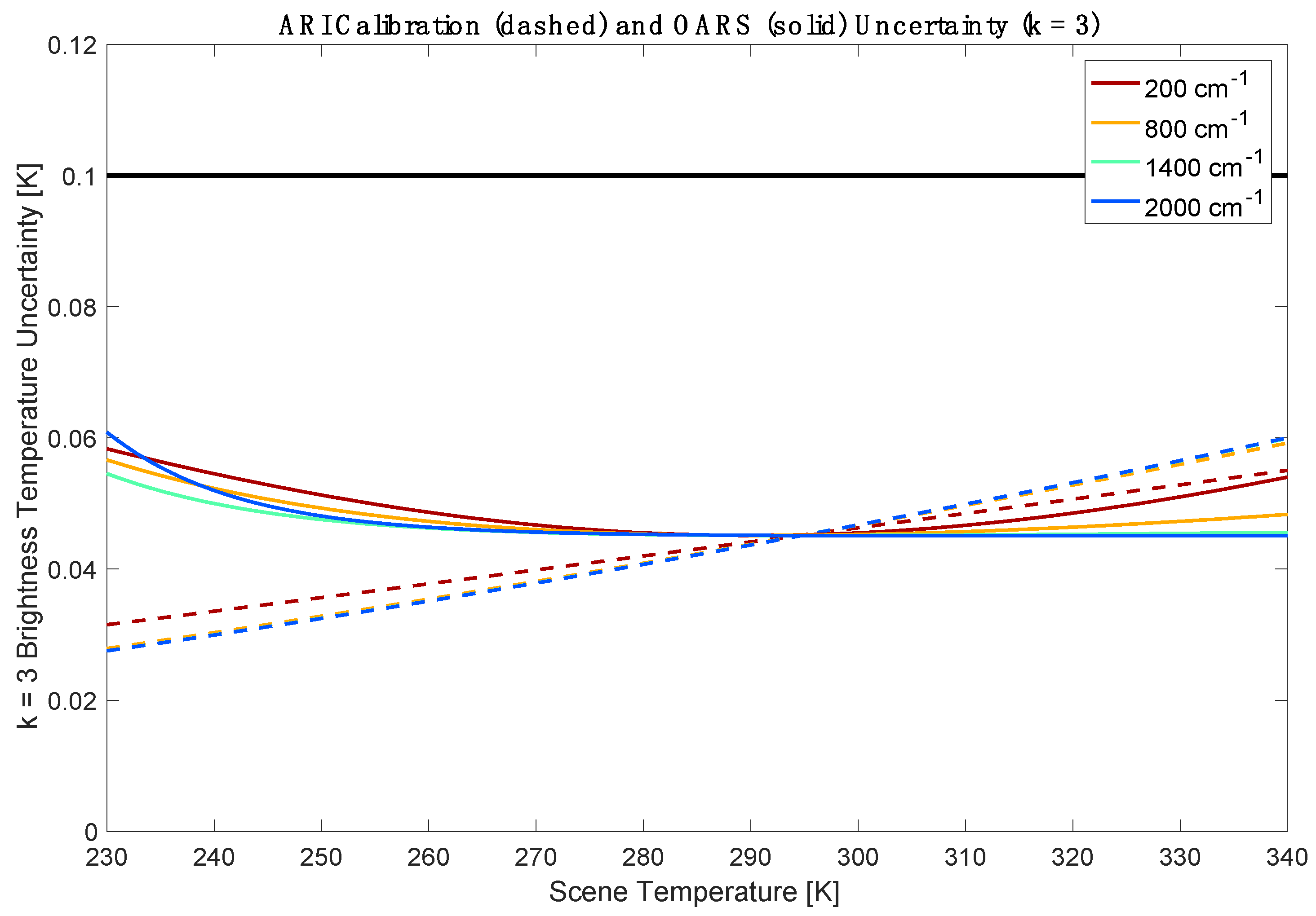
• Heat transfer conditions for the vacuum configuration are more representative of those associated with the on-orbit environment. Convection effects are significant in the laboratory environment and not present under vacuum. Increased convection results in slightly higher cavity temperature uniformity uncertainty for the calibration references in the laboratory environment, as indicated in Table 4. Since the impact is small (5 mK), a temperature uncertainty of 0.045 K for the ARI calibration sources and the OARS was used for the radiometric uncertainty analysis for all environments;
• Operation under vacuum provides complete mitigation of atmospheric absorption providing a clear assessment of the radiometric performance uncontaminated by atmospheric absorption and emission features;
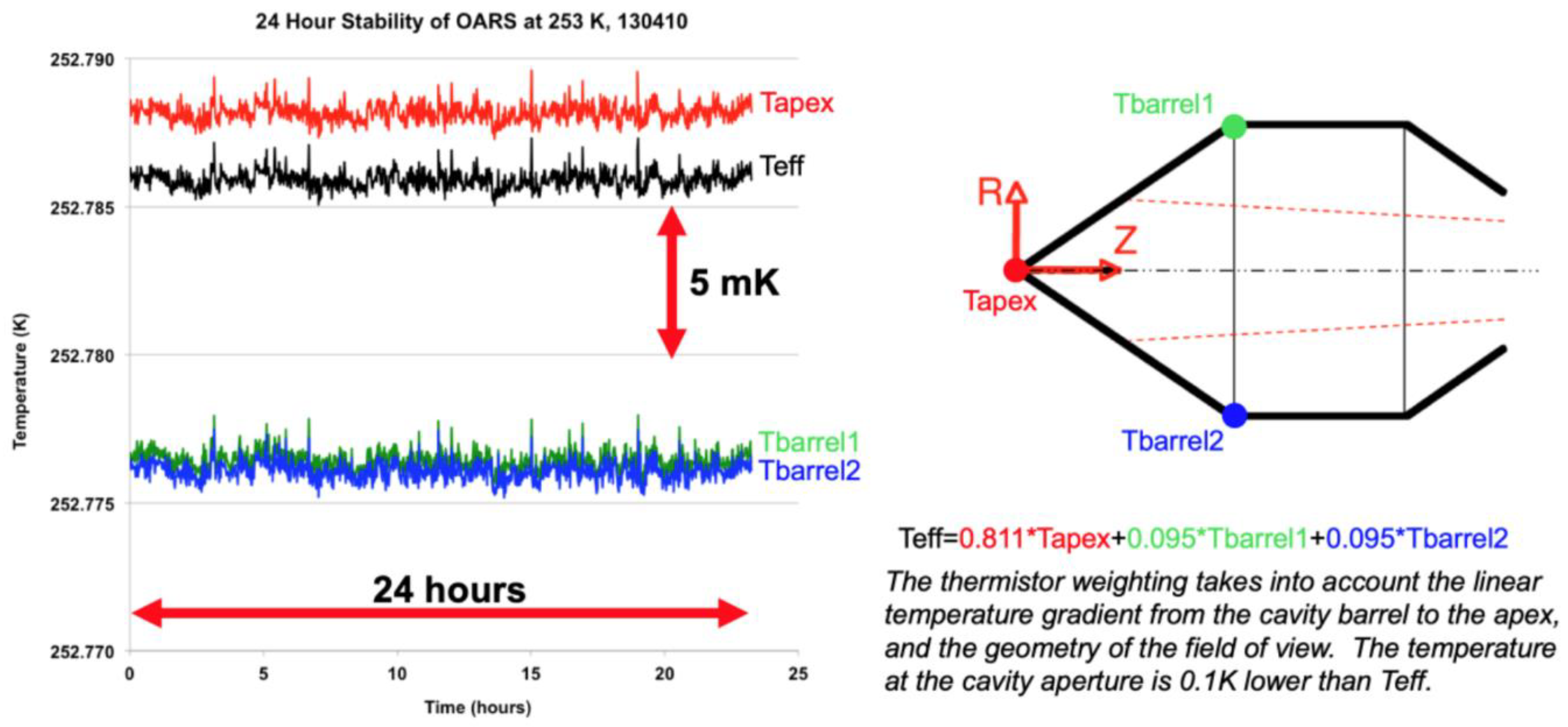
• A second OARS was fabricated for vacuum testing, which was used as a cold reference blackbody. Since there are no dewpoint concerns for vacuum testing, the OARS and cold reference blackbody could be operated at the cold setpoint limit of the blackbody controllers and the recirculating chillers. This provided not only an extended range of calibration verification temperatures, but more importantly, the reference blackbody temperature configuration is closer to the on-orbit configuration. The extended range of operation of the OARS and cold reference blackbody under vacuum conditions is +60 °C to −60 °C, with a stability of better than 5 mK over 24 h (k = 3).

Uncertainty estimates for the vacuum configuration and environment are provided in

Table 5. Uncertainty estimates used in the radiometric uncertainty analysis for vacuum configuration. All specified uncertainties correspond to a k = 3 coverage factor.

Temperatures			Associated Uncertainty
Cold Cal Ref (Cold Cal Blackbody)	$T_C$	215 K	$u(T_C)$	0.045 K
Hot Cal Ref (Warm Cal Blackbody)	$T_H$	300 K	$u(T_H)$	0.045 K
Verification Target (OARS)	$T_{OARS}$	213–333 K	$u\left(T_{OARS}\right)$	0.045 K
Reflected Radiance, Cold Cal Ref	$T_{R,C}$	295 K	$u(T_{R,C})$	4 K
Reflected Radiance, Hot Cal Ref	$T_{R,H}$	295 K	$u(T_{R,H})$	4 K
Reflected Radiance, Verification Target	$T_{R,OARS}$	295 K	$u(T_{R,OARS})$	4 K
Emissivities
Cold Cal Ref (Space Target)	$e_C$	0.999	$u(e_C)$	0.0006
Hot Cal Ref (Internal Cal Target)	$e_H$	0.999	$u(e_H)$	0.0006
Verification Target (OARS)	$e_{OARS}$	0.999	$u(e_{OARS})$	0.0006

. Figure 9 shows the radiometric uncertainties for the ARI calibration and OARS predicted radiance for the vacuum configuration, converted to equivalent brightness temperature. Figure 10 shows the combined radiometric calibration and calibration verification uncertainty estimate for the expected vacuum configuration and conditions.

The cold reference blackbody was also used for post-vacuum testing in the laboratory environment. The cold blackbody (and the OARS) need to be operated above the dewpoint temperature in the laboratory environment to avoid condensation issues. With a high-flow purge system, this lowest dewpoint achievable was approximately 240 K. The radiometric uncertainty for this test configuration (243 K cold blackbody, 300 K hot blackbody reference) is similar to the vacuum configuration for scene temperatures above 243 K and is not presented here.

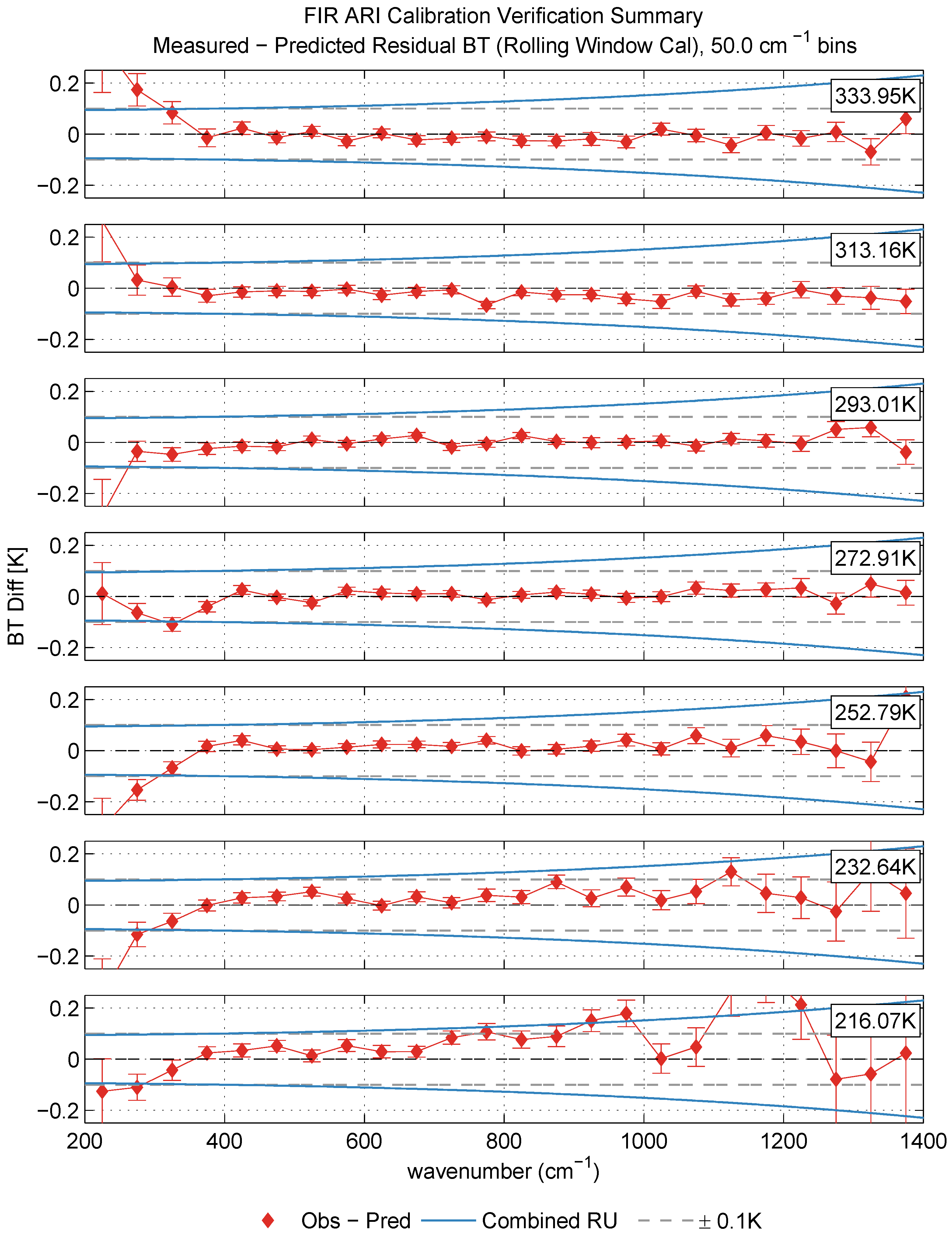
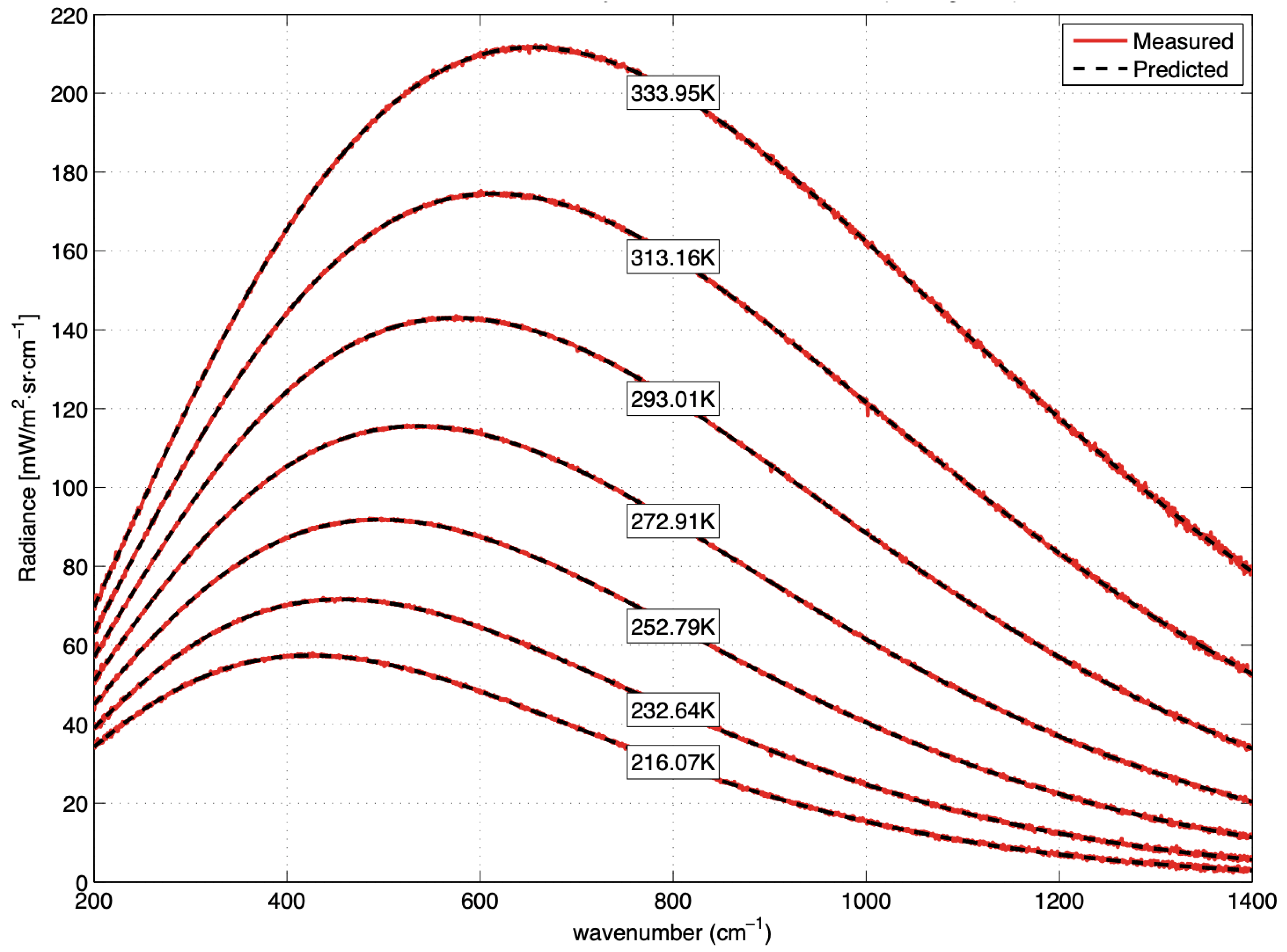
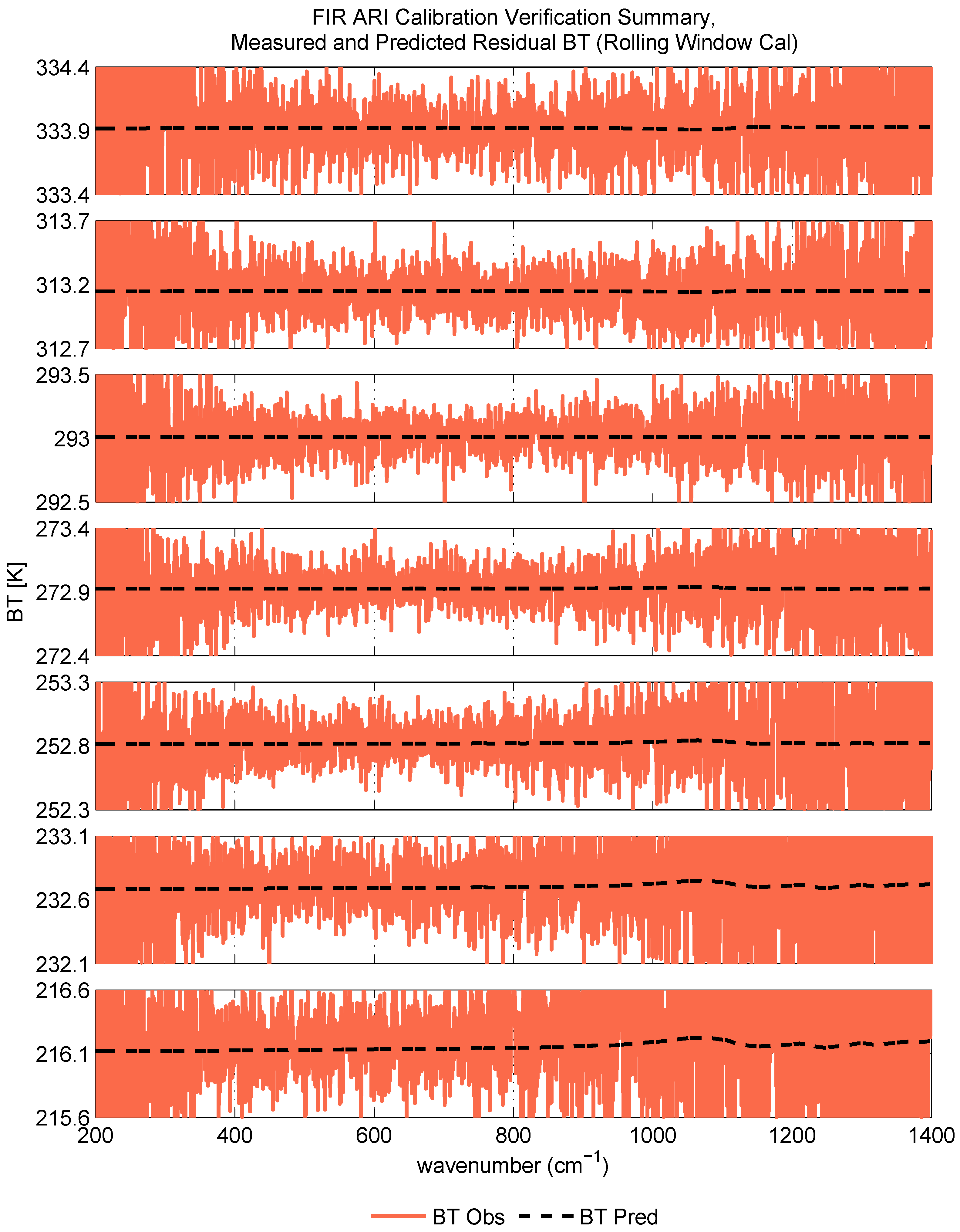
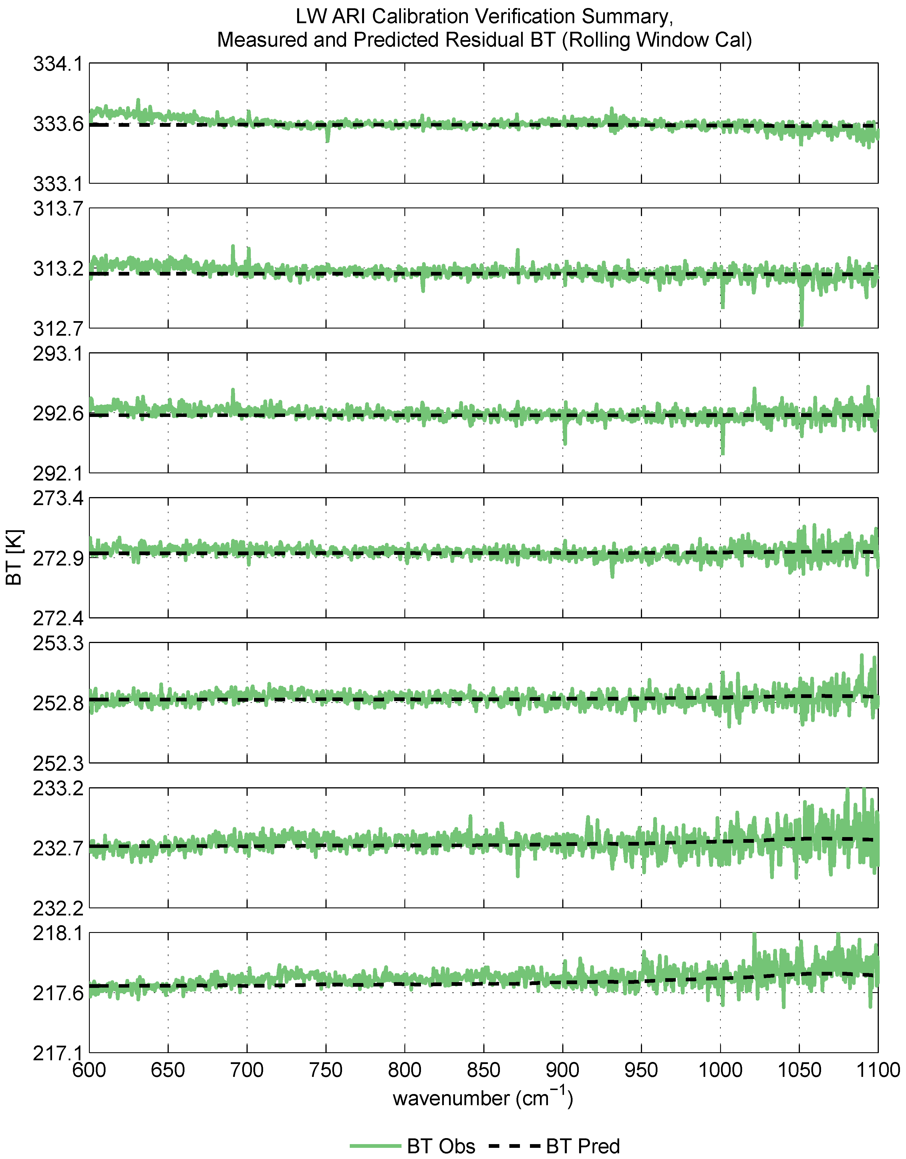
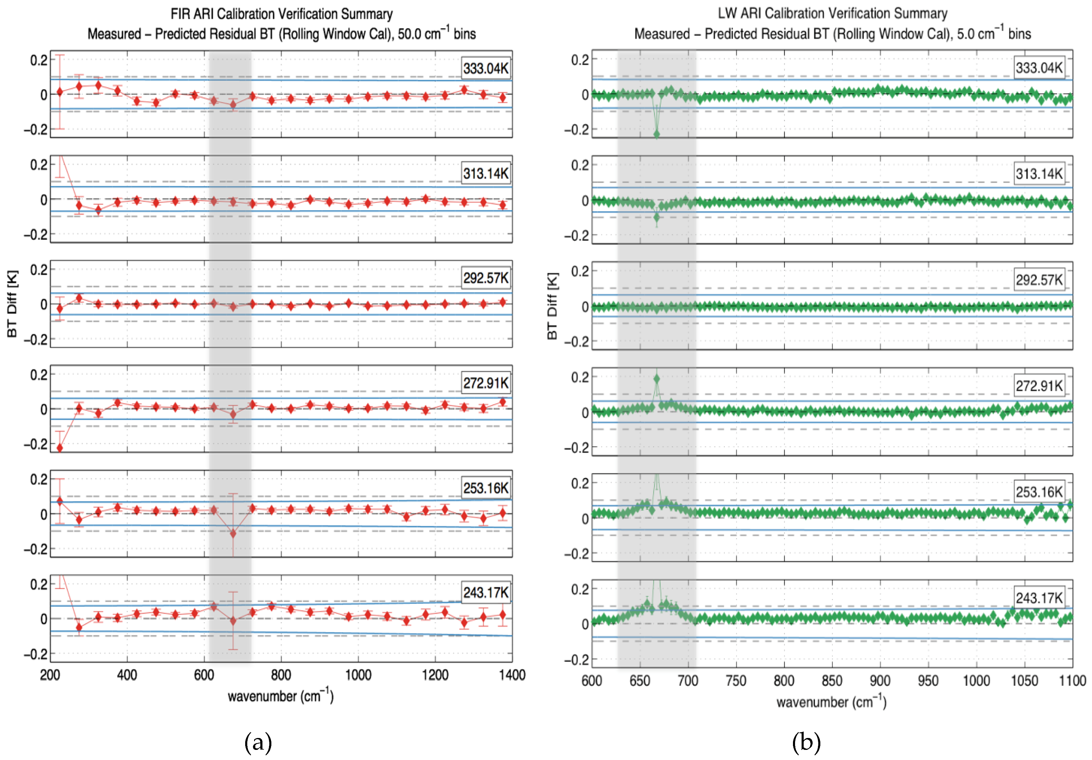
4.4. Radiometric Calibration Verification Results

The ARI calibration verification for the DTGS and longwave (LW) MCT channels presented here was completed in the vacuum calibration configuration and environment using the OARS at temperature setpoints of approximately 216 K, 233 K, 253 K, 273 K, 293 K, 313 K, and 333 K. The cold calibration reference was operated at a temperature of approximately 217 K, and the hot calibration reference at 300 K. Calibration of the data was completed using a rolling window implementation of the complex calibration method [7].

To illustrate the large range of radiance levels over which calibration validation was completed, the measured and predicted radiances for all OARS setpoints are shown for the ARI DTGS in Figure 11. Results of the calibration verification using the OARS, expressed as observed and predicted OARS brightness temperatures for the DTGS detector are shown in Figure 12. The difference between the observed and predicted brightness temperatures is shown in Figure 13. Spectral averaging has been applied to the residuals in Figure 13, with a spectral bin width of 50 cm^−1, and error bars represent a statistical error in each average. The difference between observed and predicted brightness temperature is very close to zero plus random noise in the regions with sufficient signal to noise. It can be shown that a low signal to noise ratio (SNR) threshold exists, below which bias in the calibration occurs [33,53,54]. The impact of extremely low signal to noise on calibration accuracy is discussed in detail by Taylor [33]. Despite the use of the low signal to noise formulation of the rolling window calibration equation, the impact of low signal to noise on the calibration accuracy is evident in Figure 13 in the spectral regions near the band edges, and over a wider spectral range for the case corresponding to the lowest OARS radiance (OARS temperature setpoint = 216 K). With the exclusion of the results for which low signal to noise is an issue, the results for the DTGS detector are within the prescribed radiometric uncertainty for the data collected during the ARI demonstration under vacuum.

The noise for the DTGS detector in the ARI prototype demonstration is significantly larger than what is expected for the flight design. For the vacuum demonstration, the DTGS noise is roughly a factor of 4 larger than the on-orbit noise specification due to shorter interferogram dwell times alone. As noted, a commercially available DTGS detector was used for the prototype, and improved DTGS detector sensitivity is a realistic expectation for the flight version of the instrument. Also noted earlier, due to resource constraints a beam splitter coating based on an existing production recipe was used for the ARI prototype, and it is expected that the beam splitter coating will be optimized for improved far-infrared modulation efficiency in a flight unit. Finally, the measurement duration for the vacuum duration was approximately 24 h for each OARS temperature. The number of observations averaged for the climate radiance products will be significantly larger, with a corresponding reduction in noise via the larger averages. With these considerations, the signal to noise for the DTGS channel is not expected to be an issue for the flight unit and the on-orbit climate benchmark measurement.

The observed and predicted OARS brightness temperatures for the LW MCT detector are shown in Figure 14 and the brightness temperature residuals are provided in Figure 15. Spectral averaging has been applied to the residuals, with a spectral bin width of 5 cm⁻¹ and the error bars represent the statistical error in each average. Nonlinearity correction has been applied for the LW MCT. The results are within the predicted combined radiometric calibration and calibration verification uncertainty. A small bias, associated with the stray light issue that was resolved after vacuum testing, is evident for the 313.16 K and 333.61 K OARS data collection results. The radiometric calibration validation results after implementation of the solution to the stray light issue are provided in Figure 16. For the post vacuum test results, the testing was completed in the laboratory environment under a dry air purge. Due to laboratory dewpoint considerations, the OARS was limited to an operating range of 243–333 K, and the cold reference blackbody was operated at 243 K. The predicted radiances for the OARS do not include atmospheric absorption calculations and as a result, the 15 μm CO₂ band absorption signature is evident in the residual.

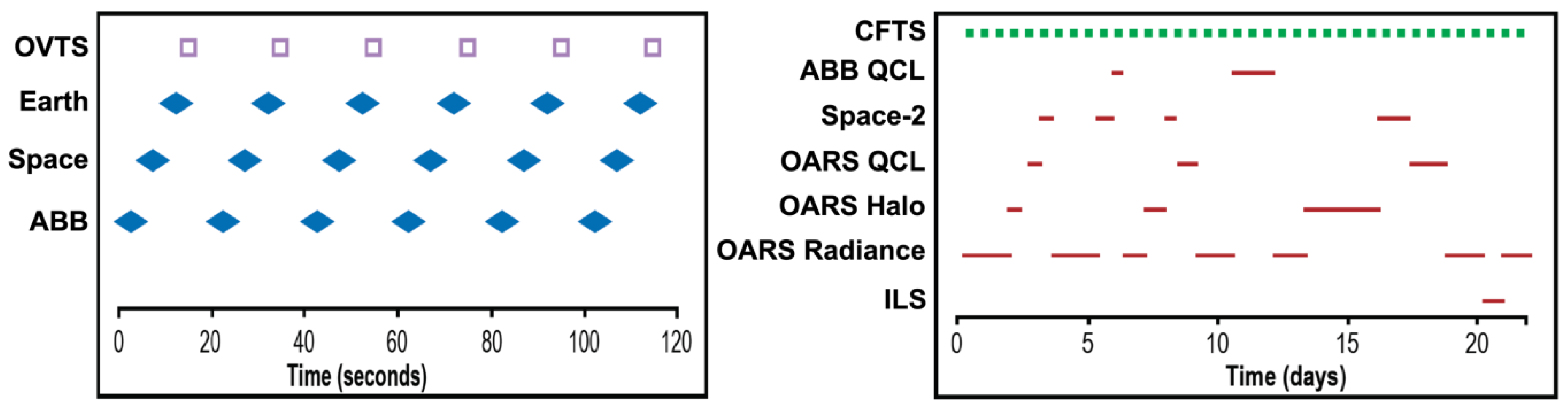
5. The On-Orbit Verification and Test System (OVTS)

As described earlier, the ARI Calibrated Fourier Transform Spectrometer (CFTS) is calibrated on-orbit in the traditional way using an ambient blackbody and a space view. The ARI also includes a completely independent set of end-to-end calibration verification measurements that make up the On-Orbit Verification and Test System (OVTS). The OVTS consists of an On-Orbit Absolute Radiance Standard (OARS) and modules for measuring blackbody cavity emissivity and Instrument Line Shape (ILS) using a Quantum Cascade Laser (QCL). The same 45° scene mirror that is rotated to expose the CFTS to its calibration sources is used to select OVTS views. The scene mirror is also used to direct the QCL beam into the OARS or Ambient Blackbody for emissivity measurements at 9.5 µm, or into an integrating sphere for ILS measurements. This section describes each of the elements of the OVTS and concludes with an on-orbit observation scheme that illustrates how the verification measurements are interleaved with the climate observations.

5.1. On-Orbit Absolute Radiance Standard (OARS)

The On-Orbit Absolute Radiance Standard (OARS) is a measurement standard that provides traceability to the SI, the International System of units [20,21,22,23]. It is a variable temperature (−50 to 50 °C), high emissivity (>0.998–0.999), cavity blackbody that serves as a standard radiance source based on the fundamental quantum mechanical theory of the Planck function. The Planck function radiance applies to a perfectly emitting blackbody (unit emissivity) and depends only on temperature and wavenumber (or wavelength). The small deviation of the OARS radiance from a Planck function because of its non-unit emissivity is handled by knowing its emissivity quite accurately (order 0.1%) and accounting for its reflection of background radiation. Because of the high emissivity, an uncertainty of several degrees in the effective background radiative temperature is acceptable. For ARI, the wavenumber scale is accurately maintained by the Fourier Transform Spectrometer (FTS) operating principle that uses a temperature-controlled diode laser to control Optical Path Difference sampling and is calibrated using the signatures of atmospheric absorption lines with well-known spectral locations. In addition, the spectral instrument line shape (ILS) is measured on-orbit.

5.1.1. OARS Temperature Calibration

A section view schematic of the key features of the OARS design is shown in Figure 17. The light-trapping cavity shape is coated with Aeroglaze Z306 diffuse black paint, recently improved by adding carbon nanoplatelets to enhance emissivity out to 50 µm. The heated cavity temperature is measured with five Thermometrics SP60 thermistors, with absolute temperature calibration provided by three embedded phase transition cells (mercury, water, and gallium). The heated cavity is cold-biased to its fluid-controlled shroud; the spaceflight OARS will use a conductive coupling to a cold heat sink in place of the circulating temperature-controlled fluid. The Heated Halo located in front of the cavity is used for periodically measuring cavity emissivity to within an accuracy of 0.0006 (k = 3) [26,27]. The OARS cavity design is a derivative of an earlier UW development for NASA’s Geostationary Imaging Fourier Transform Spectrometer (GIFTS) [41,55]. Under NASA IIP funding the OARS with its phase transition cell and Heated Halo technologies were brought from TRL 3 to 6.

The concept for using miniature phase transition cells to calibrate imbedded blackbody cavity thermistors in the ARI Prototype instrument is illustrated in Figure 18, which shows a typical transient temperature response from one of the blackbody cavity thermistors during a gallium (<30 mg) melt event [20,21,22,23]. At the start of the melting process, the blackbody cavity is brought to thermal stability in the constant temperature mode about 50 mK under the expected phase change temperature. Then the blackbody controller is switched into constant power mode using a power level that would bring the cavity to about 100 mK above the expected phase change temperature, and provide a melt duration of 6500 s. If no gallium were present, the cavity would follow an exponential temperature rise to a new equilibrium temperature; however, even in the presence of a small quantity of gallium the cavity heater power goes into melting the gallium when it reaches the melt temperature—creating a melt plateau on the temperature vs time plot. As the time taken to pass through the melt plateau increases, the mid melt temperature more closely approaches the theoretical melt temperature to the reference material. This is illustrated, again for gallium, in Figure 19.

It has been shown that the asymptotic characteristic curve used to fit the mid melt temperature versus melt duration data shown in the right plot of Figure 19 is unique and invariant for a given melt material and design implementation. This is important on-orbit because repeated long-duration melts are not necessary to establish calibration. Even though the thermal design of the OARS provides immunity to the expected on-orbit variations in instrument temperature, which allows melts to be conducted throughout an entire orbit, establishing the characteristic curve with mostly shorter melts (on the order of 2000 s) is all that is necessary. The characteristic curve also served as an important metric in the validation of the housing design and greatly simplified the extensive accelerated life testing that simulated 7 years on orbit [20,23].

Extensive testing has shown that the calibration temperatures associated with the three different melt materials can be established to within 10 mK using the transient signature approach, see Figure 20. A thermistor temperature sensor is calibrated using this scheme by measuring its resistance during the mid-melt plateau. With the aid of the characteristic curve, a calibration temperature can be assigned and associated with this resistance. A continuous temperature scale accurate to better than 16 mK (k = 3) is established by using each of the three melt points to constrain the three coefficients of the well-established Steinhart–Hart thermistor sensor equation [20]. The thermal design of the blackbody and long duration of the melt transient, lead to “isothermal” conditions in the cavity during a melt, keeping the gradients between the melt materials and the thermistors under calibration to typically less than 2 mK.

The temperature gradient and 24-h stability of the OARS at a setpoint of −20 °C (with an environmental temperature of +20°) are shown in Figure 21, under vacuum conditions. Temperatures from three thermistors, located in the blackbody cavity as shown at right, are plotted along with the effective radiating temperature (T_eff) of the blackbody. The maximum gradient in the critical conical section of the blackbody is on the order of 15 mK for the case shown, with a cavity setpoint temperature of −20 °C and the ARI instrument temperature at 20 °C. Because these gradients are driven mainly by conduction, they are expected to double to no more than 30 mK at the worst-case setpoint temperature of −60 °C, well under the allocated gradient of 0.1 K. The 24-h plot illustrates excellent thermal stability during the test. The effective temperature is computed by weighting the cavity thermistors following the formula at the bottom of the figure. The weighting factors were determined by convolving the interferometer CFTS instrument viewing geometry with the cavity thermal gradient geometry.

The overall estimate for temperature uncertainty for the OARS on-orbit is shown in

Table 6. OARS temperature uncertainty budget. Refer to Siwek et al. [42] for further details on the thermistor stability.

Source of Error	Temperature Uncertainty [K] (3-σ)
Thermistor Temperature Calibration Uncertainty
Melt Plateau Determination	0.010
Transfer of Melt Cell to Thermistor Uncertainty (gradients during cal.)	0.002
Thermistor Calibration Equation Interpolation Error Between Cal. Pts.	0.016
Cavity Temperature Uniformity Uncertainty
Cavity to Thermistor Gradient Uncertainty (1/2 of max expected gradient)	0.015
Thermistor Wire Heat Leak Temperature Bias Uncertainty *	0.020
Paint Gradient (due to radiative coupling to surrounding temperatures)	0.018
Stablilty Between Calibrations
Blackbody Thermistor (From [42] with factor applied for configuration differences)	0.005
Blackbody Thermistor Readout Electronics	0.005
Effective Radiometric Temperature (Teff) Weighting Factor Uncertainty
Monte Carlo Ray Trace Model Uncertainty in Determining Teff	0.025
(radiometric error that accounts for non-isothermal cavty temperature) (On-Orbit cases improved due to additional modelling)
RSS Combination	0.045

* Due to conductive coupling of leads to a temperature different that the cavity.

. This budget includes the 3-σ uncertainty contributions from the thermistor calibration using phase-change cells, the cavity temperature uniformity (during operation), the thermistor and readout electronics stability between calibrations, and the determination of the thermistor weighting factors used to calculate the blackbody effective radiating temperature from the cavity measured temperatures. The RSS combination of all the uncertainty sources in the table indicates an on-orbit total blackbody temperature uncertainty of 45 mK (k = 3). This value used in the end-to-end uncertainty budget for the ARI instrument.

5.1.2. OARS Spectral Emissivity Measurement

To avoid having to assume emissivity stability on-orbit, a system called the Heated Halo has been devised to measure the broadband spectral emissivity of the OARS cavity. Figure 22 presents the configuration and method used to make these measurements, which are described in detail by Gero [26,27]. The heated halo is heated to 70 °C above the blackbody cavity that is at ambient temperature (near 20 °C). Baffling is configured so that the halo is visible to the ARI CFTS spectrometer only via reflection from the cavity. Equation (10) defines the radiance measured by the CFTS when viewing the OARS equipped with the Heated Halo. The measured radiance consists of two components: (1) the radiance emitted from the OARS cavity, and (2) the radiance reflected from the OARS cavity.

$$L_{OARS}=e_{OARS}B(T_{OARS})+\left(1-e_{OARS}\right)\left[F\cdot B(T_{halo})+\left(1-F\right)\cdot B(T_{bg})\right]$$

(10)

All of the terms on the right side of Equation (10) are known except for the cavity emissivity, $e_{OARS}$. B(T_OARS) is the Planck radiance emitted directly from the blackbody cavity. The view factor from the cavity to the heated halo is F and can be accurately calculated using traditional radiation transfer methods. B(T_halo) is the Planck radiance from the halo, and B(T_bg) is the background radiance. Equation (10) can be rearranged to solve for the cavity emissivity:

$${\langle 1-e_{OARS}\left(t\right)\rangle }_t={\langle \frac{L_{OARS}\left(t\right)-B(T_{OARS}\left(t\right))}{L_{refl}-B\left(T_{OARS}\left(t\right)\right)}\rangle }_t$$

(11)

In Equation (11), t is the time of the measurement, and the radiance emitted from the Heated Halo and the background that the CFTS observes reflected from the cavity has been combined into a single term, L_refl:

$$L_{refl}\left(t\right)=F\cdot B(T_{halo}\left(t\right))+\left(1-F\right)\cdot B(T_{bg}\left(t\right))$$

(12)

Equation (11) can be used to calculate emissivity at each time (t), following an instrument calibration cycle (~20 s). Using this approach, the individual emissivity measurements can be averaged over long periods to reduce noise in the measurement, eliminating the need for thermal stability over the entire duration of the measurement.

Figure 23 shows emissivity measurements of the OARS Cavity from the Heated Halo method, using a fully integrated ARI instrument operated under laboratory conditions. Test results and careful uncertainty analysis of the heated halo implementation for ARI show that the emissivity can be measured to about 0.06%, better than the 0.1% required for CLARREO [26,27]. The dashed red line at 0.998 represents the cavity threshold emissivity level needed for the Heated Halo measurement uncertainty to be below the target of 0.06%. The red curve is from measurements of a cavity painted with Aeroglaze Z306 and the blue line is from a cavity painted with this paint doped with graphene nanoplatelets, recently added to enhance the emissivity out to 50 microns—the ARI measurement limit. The discrete data points shown in the plot are from independent measurements conducted at NIST using three different techniques and show good agreement with the Heated Halo results. The measurements were made using blackbodies from the Atmospheric Emitted Radiance Interferometer (AERI) program [9,10] that are scaled geometric equivalents to the OARS cavity and coated with the same Aeroglaze paint. The three NIST measurements [56] were made using the: Thermal-Infrared Transfer Radiometer (TXR) [57]; Complete Hemispherical Laser-based Reflectometer (CHILR) [58]; and Advanced Infrared Radiometry and Imaging (AIRI) facility [59].

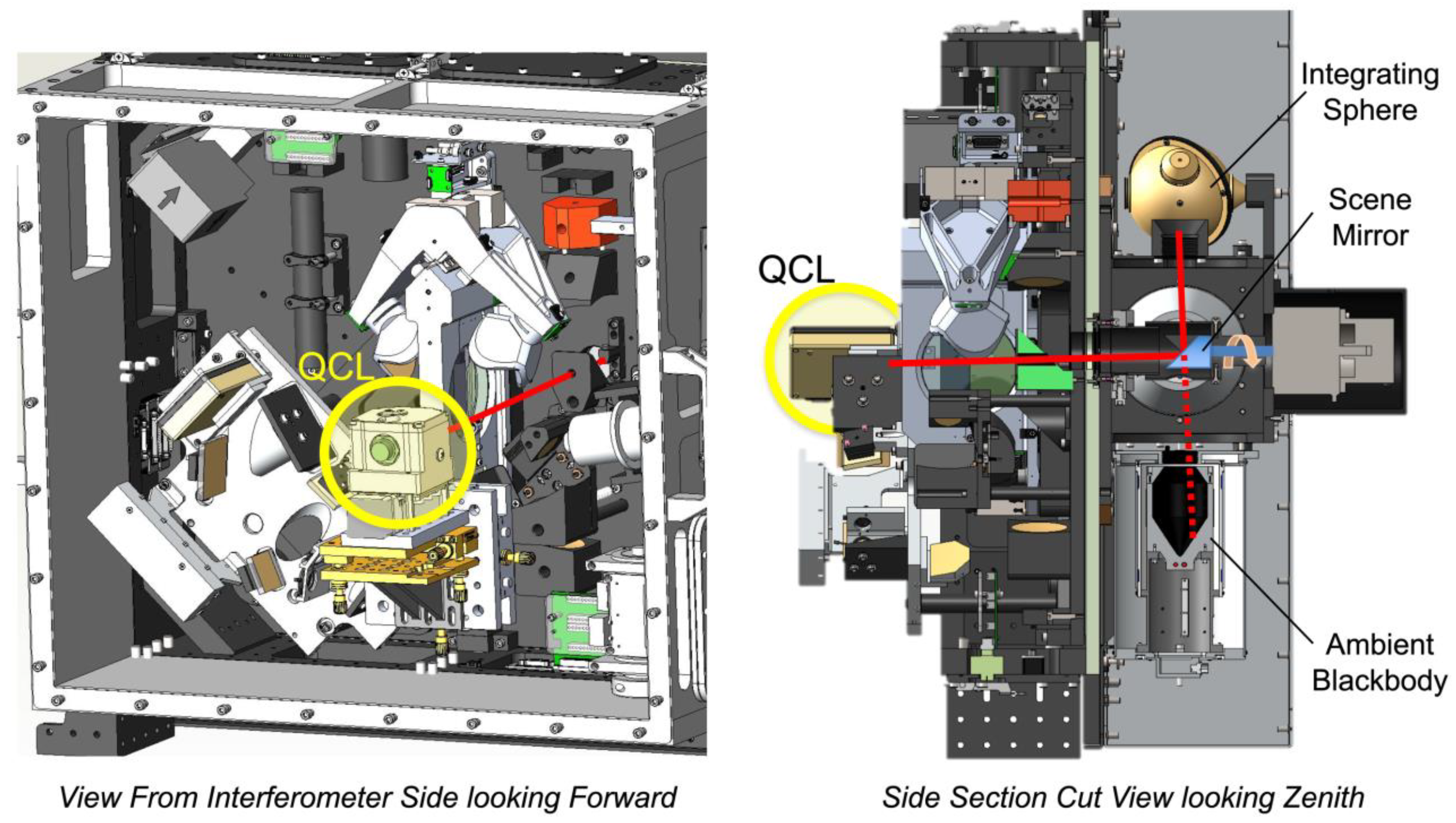
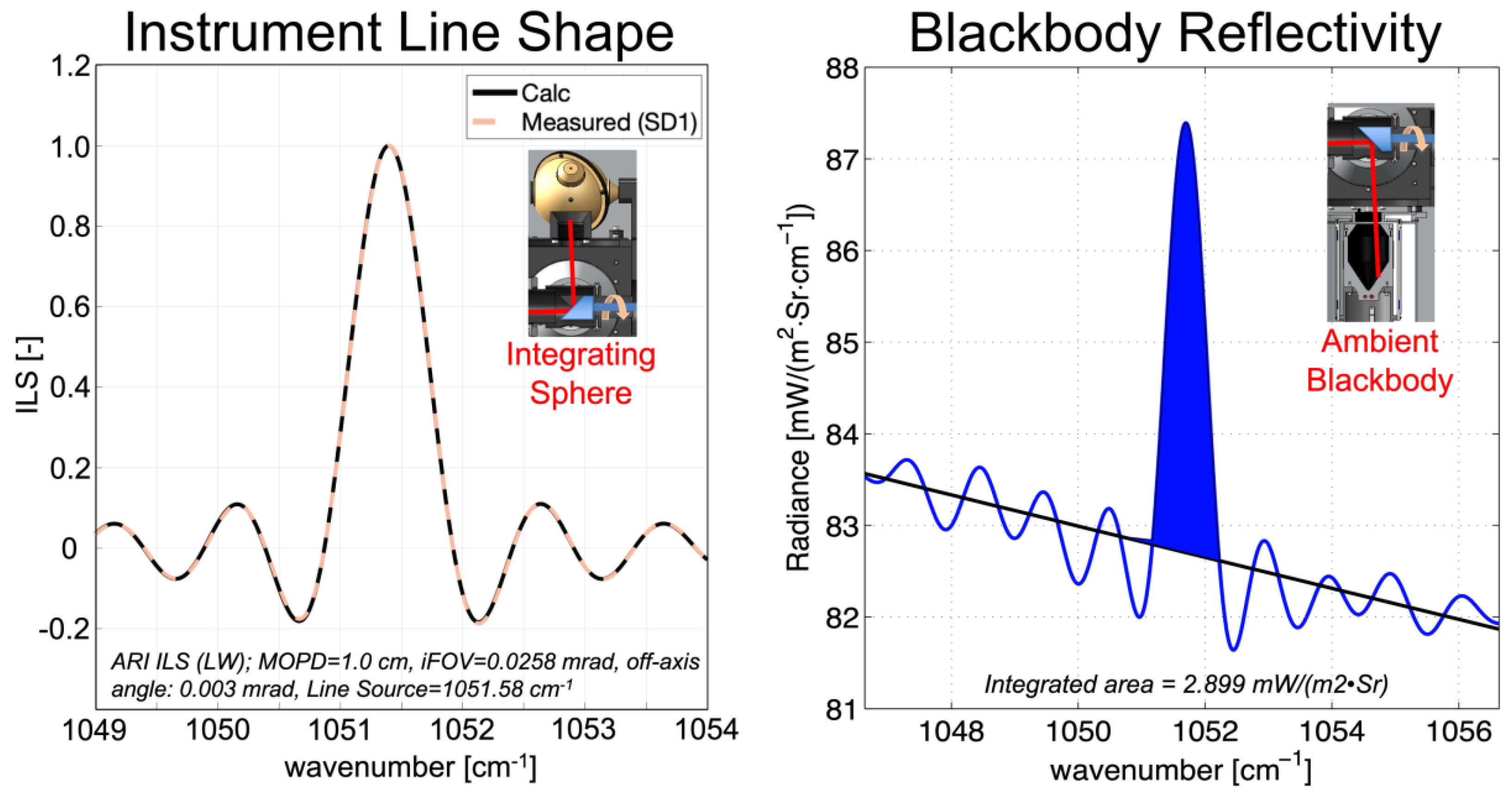
5.2. Blackbody Cavity Emissivity and Instrument Line Shape Measurement Using a Quantum Cascade Laser

The OVTS includes a Quantum Cascade Laser (QCL) with an output wavelength of 9.5 µm to measure the Instrument Line Shape (ILS) and monochromatic reflectivity of the OARS and Ambient Blackbody cavity. The QCL was packaged and characterized by the Anderson group at Harvard University [60] and then integrated into the ARI instrument at Wisconsin. Figure 24 illustrates the flight configuration of the QCL which is positioned in the back of the fore optics and injected into the center of the 45° Scene Mirror through a hole in the 1st optical flat (the periscope mirror). The scene mirror is used to direct the QCL beam to the target of interest: either the Integrating Sphere, OARS, or Ambient Blackbody.

Figure 25 presents an instrument ILS and an Ambient Blackbody reflectivity measurement that were obtained using the QCL. These measurements were made prior to the integration of the QCL into the flight-like configuration shown in Figure 24. For these measurements, the QCL was injected directly into the target of interest from the front of the instrument, while bypassing the Scene Mirror. Similar results are expected with the QCL in the flight-like configuration, which introduces only one additional flat into the QCL beam path.

The ILS measurement shown in Figure 25 (solid) is in excellent agreement with the standard self-apodization line shape (dashed), which follows from the field stop geometry that limits the spread of angles in the interferometer to dθ. The resulting smear of the Optical Path Difference x = x₀ cos θ by dx = x₀ d (cos θ) = −x sin θ dθ for each field point θ determines the ILS in the spectral domain. While the type of interferometer used on ARI has proven to be highly stable, having this type of information on orbit provides verification and would allow any significant geometry change to be detected and accounted for.

The QCL blackbody reflectivity measurements (illustrated in Figure 25 for the Ambient Blackbody) provide a way to also monitor any unexpected changes in the ABB emissivity on-orbit by comparison with the OARS. The QCL beam is positioned to hit the conical portion of the blackbody cavities directly viewed by the CFTS, a location where the signal has been shown to have a weak dependent on illumination geometry. While the beam does not fill the area viewed by the CFTS, it directly illuminates a large enough area to be representative (about 25%). Because of the high emissivity of the ARI blackbodies, even a 10% change in the measurement of the QCL reflected power (which is easily achieved by measuring the blue area in the figure) provides a relative comparison of 0.0003 emissivity change. In fact, since the ILS measurements provide an accurate measure of the QCL power, a useful estimate of the absolute emissivity can also be deduced from these measurements combined with cavity modeling.

5.3. Other OVTS Capabilities

An additional feature of the OVTS is the provision of a second space view, clocked 45° from the primary space view, that is used to characterize any artifacts due to polarization. These artifacts are fundamentally minimized by important features of the instrument design that include uncoated gold reflective optical elements, and clocking of the Earth, Space, Ambient Blackbody, and OARS targets at 90° intervals, at the polarization null points. In addition, all targets are viewed by the FTS via the same 45° rotating scene mirror.

Another feature of the OVTS is used to check for any subtle out-of-field obstructions in the instrument field of view while viewing the Earth or Space views. This is accomplished by commanding (on/off) annular shaped heaters at the limiting apertures for the view in question.

5.4. Concept of Operations Employing Climate Measurements With on-Orbit Verification

Figure 26 illustrates the concept of operations for the ARI instrument on-orbit, which interleaves climate measurements of the Earth with the different verification elements of the OVTS. The ARI continuously collects an interferogram every 5 s. In the diagram at the left of the figure, the instrument scene mirror is used to sequence through a calibration cycle (Earth, Space, and Ambient Black Body) and a view of the OVTS, every 20 s. Over a period of 22 days, different elements of the OVTS are viewed as shown in the diagram at right. Over this period, the OARS is stair-stepped over a temperature range from −50 °C to 50 °C. If desired, melts of the phase changes cells can be obtained during dwells at the three melt temperatures of −38.9, 0, and 29.8 °C, for mercury, water, and gallium respectively.

The On-Orbit Verification and Test System is what really sets the ARI apart from previously deployed instrumentation employing on-orbit calibration. It provides SI radiance and temperature scale references and verification testing on-orbit that either makes sure the on-orbit calibration is stable or determines how to correct it.

6. Radiance Intercalibration Traceability for Improving the Accuracy of Operational IR Sounding Instruments

There are many Earth system investigations of weather- and climate-related processes and climate change that rely on observations that do not have the inherent accuracy and traceability desired for the intended use. That is, data from sensors designed and tested based on weather-related specifications are frequently used in studies to understand and track climate, yet often lacking the required basic measurement characteristics. Furthermore, today’s state-of-the-art numerical weather prediction and atmospheric sounding applications are increasingly demanding on weather satellite sensor absolute accuracy, internal consistency (e.g., consistent calibration across scan angle or detector array), and stability. Therefore, a key challenge that spans innumerous Earth science applications is to understand, and improve if possible, the accuracy of NOAA, NASA, and international satellite products. In particular, a challenge is to improve the radiance calibration accuracy of the large suite of infrared sensor observations including those from, for example, the Atmospheric Infrared Sounder (AIRS), Infrared Atmospheric Sounding Interferometer (IASI), Cross-track Infrared Sounder (CrIS), Moderate Resolution Imaging Spectroradiometer (MODIS), Visible Infrared Imaging Radiometer Suite (VIIRS), Advanced Very High Resolution Radiometer (AVHRR), High-Resolution Infrared Radiation Sounder (HIRS), and Geostationary Operational Environmental Satellite (GOES). Specifically, the goal is to increase the accuracy of the infrared observations by factors ranging from 3 to 10, approaching 0.1 K 3-σ uncertainty. The resulting improved calibration and characterization of the calibration uncertainties will provide benefits in two main areas: (1) improved radiances and derived products from the individual intercalibrated sensors, and (2) the ability of the intercalibrated radiance observations to contribute to the construction of a climate radiance benchmark.

6.1. The Need for Improved Infrared Observation Calibration Accuracy via Intercalibration with a Reference Sensor

CLARREO has the potential to provide high accuracy measurements with on-orbit SI traceability that will form the backbone of the satellite intercalibration system, making the larger suite of satellite observations more useful for both weather and climate applications. This approach is in line with the overall strategy promoted for several years. For example, the need for this type of reference observation capability is recognized and discussed in Ohring et al. 2007 [12]. The need was also recognized when NASA identified CLARREO as a Tier 1 mission in its 2007 Decadal Survey. Also, as summarized in the 2013 WMO/CEOS/CGMS report “Strategy Towards an Architecture for Climate Monitoring from Space” (Dowell et al. 2013) [61]: “To characterize climate and climate change, data need to be accurate and homogeneous over long time scales. The signals important for the detection of climate change can easily be lost in the noise of a changing observing system. This enforces the need for continuity in an observing system, where observations can be tied to an invariant reference. Such a system needs to be maintained over at least several decades and beyond. It is with these boundary conditions that a climate monitoring architecture needs to be formulated.” Similarly, the 2015 NASA report “Continuity of NASA Earth Observations from Space: A Value Framework” highlighted the need for measurement continuity. Via intercalibration, CLARREO offers the ability to assess measurement uncertainty of infrared sensors as well as the ability to improve concurrent sensors calibration and therefore provide improved measurement continuity.

Currently, the international intercalibration community, organized around the Global Space-based Inter Calibration System (GSICS) [62], utilizes IASI, AIRS, and CrIS to serve as “reference sensors” for the intercalibration of other infrared observations, despite the relatively large uncertainty in these observations and the lack of in-orbit verification and traceability that is needed for the rigorous metrology required for climate studies and associated societal decisions. Other than CLARREO, there are no other existing or planned programs that will provide this capability. This is a challenge that must involve improved spaced based observations, and other existing and planned programs lack the high accuracy and in-orbit traceability required for this challenge. Hewison et al. 2020 [63] describe the benefits of extending GSICS to tie Satellite Radiances to an absolute scale, which is based on the availability of future sensors termed “SI-Traceable Satellite instruments” or SITSATs, such as ARI.

6.2. CLARREO Observational Requirements and Its Ability to Serve as an Infrared Intercalibration Reference

Previous sections of this paper document the performance of the ARI. Summarizing, it is expected to provide infrared observations with absolute calibration with uncertainty better than 0.1 K 3-σ and with in-orbit calibration verification. The observations are also well suited for intercalibration, with full contiguous spectral coverage from 3.5 to 50 microns, high spectral resolution, and good radiometric noise performance.

The characterization of the ability of CLARREO to serve as an infrared intercalibration reference is provided in Tobin et al. 2016 [17]. The intercalibration strategy includes the intercalibration of CLARREO with the sun-synchronous hyperspectral sounders (AIRS, CrIS, IASI), followed by the existing GSICS strategy of intercalibration of these sounders with various broadband infrared sensors on sun-synchronous and geostationary platforms. The intercalibration capability is investigated for a 90-degree polar orbit CLARREO mission and for a Pathfinder mission on the International Space Station. For both of these cases, the CLARREO intercalibration performance is very good, with 3-σ intercalibration uncertainties less than 50 to 100 mK (depending on the wavelength region considered and whether intercalibrating with IASI versus AIRS or CrIS) obtained after accumulating several months of collocated observations.

Here, we present the metrology considerations for quantifying the traceability of the intercalibration process. The fundamental challenge to achieving optimized comparisons and ascribing accurate uncertainty estimates is defining how to handle errors related to spatial and temporal mismatches. The key properties of spatial mismatches from the simulations using MODIS images are illustrated in Figure 27.

The mathematical approach to quantifying the radiance uncertainty of each Simultaneous Nadir Overpass (SNO) due to sampling differences, based on the properties shown in Figure 27, is quite straight forward (although, beware that the result in our first two publications is incorrect [17,64], as explained below). Assume that the mean of M sounder samples that fall within the j^th ARI circular footprint are used to represent the coincident sounder estimate of the ARI measurement, $C^{SDR}=\frac{{\sum }_{i=1}^M{y}_i}{M},$ where the spatial uncertainty associated with each spectral sample y is Gaussian with standard deviation ${\sigma }_j$. Then, to make use of the statistical properties of sounder samples, it is assumed that the Big Circle representing the ARI measurement can be exactly filled by N sounder samples (think of it as geometrically a big square with aligned square sounder FOVs). The Big Circle mean measurement representing ARI can be written as $C^{ARI}={\sum }_{i=1}^N{y}_i/N$. The variance of the difference for a given intercomparison j is then

$$\begin{array}{cc}\hfill \mathrm{var}\left(C^{SDR}-C^{ARI}\right)& =\mathrm{var}\left[\frac{{\displaystyle {\sum }_{i=1}^M{y}_i}}{M}-\frac{{\displaystyle {\sum }_{i=1}^N{y}_i}}{N}\right]\hfill \\ & =\frac{{\sigma }_j^2}{M}-\frac{{\sigma }_j^2}{N}\hfill \\ & =\left(1-\frac{M}{N}\right)\frac{{\sigma }_j^2}{M}\hfill \end{array}$$

(13)

Note that this form for the variance (or square of the uncertainty due to sampling differences) makes physical sense, because the sampling uncertainty goes to zero when M = N and blows up when there are no sounder samples (M = 0). The analogous equation in [17] used N in the denominator instead of M.

This spatial sampling error formalism can be used, combined with noise and similar temporal sampling error estimates, to optimally weight mean SNO differences [17]. The weights are the normal inverse of the total error variance [w_j = 1/(total error variance for SNO_j)], and yield a rigorous uncertainty estimate [=$1/\sum {\omega }_j^{1/2}$]. This approach results in a rigorous mean difference and uncertainty, with no clear sky selection or other SNO filtering! The benefit of not have to perform clear sky determinations or SNO filtering of any other kind is that these processes are inherently subjective and therefore lack quantitative uncertainty propagation.

Finally, applying this technique shows that a single CLARREO in a true polar orbit can achieve Intercalibration uncertainties for the CrIS and AIRS sounders (for which M/N = 0.55) of less than 0.05 K in 6 months, even assuming a reasonably large CLARREO noise and for a window channel where spatial non-uniformity is largest (see Figure 28).

This shows that intercalibration can be used to transfer the higher CLARREO accuracy, proven on-orbit, to other concurrent sensors with rigorous traceability, and that a single ARI Pathfinder instrument could lead to a very important climate benchmark. Future ARI launches could then establish long-term trends with unprecedented accuracy.

7. Conclusions

The overall conclusion of this paper is that the new technologies and implementation approaches demonstrated and tested with the ARI instrument have proven the capability needed to justify a spaceborne pathfinder that would initiate an ongoing sequence of missions to better quantify the long-term climate trend of Earth emission from orbit. More specifically, we conclude that

• The scientific value and societal benefits of spectrally resolved Earth emission spectrum measurements with ultra-high and proven accuracy have been well established by the NASA CLARREO Science Definition Team and related activities. Wielicki et al. [15] have shown that both emitted radiative trends and trends in temperature and water vapor distributions can be quantified at close to the observing limit set by natural variability using the type of measurements defined here, and that a series of this type of SI-based benchmark measurements will help limit the uncertainty of climate models. Both the information content and the accuracy significantly exceed that of current and planned total broadband climate observations including the Libera mission, recently selected by NASA under its new Earth Venture Continuity program. Further, regarding the benefits of the far-infrared coverage of ARI, it will substantially augment the valuable capability to be offered by the new NASA PREFIRE (Polar Radiant Energy in the Far-InfraRed Experiment) and ESA FORUM (Far-infrared Outgoing Radiation Understanding and Monitoring) missions. The ARI spectral resolution is substantially higher than that of PREFIRE, and the ARI radiometric accuracy and capability for on-orbit end-to-end calibration verification with direct traceability to absolute standards is not offered by any other mission.
• NASA Instrument Incubator Program (IIP) developments and follow-on refinements have resulted in a mature ARI instrument design that is ready for mission implementation. The IIP took our early design concepts for making spectrally resolved climate observations (including verifying them on-orbit using an SI standard and extensive testing) and advanced them to a NASA TRL 6 design using a demonstration unit with a short technological path to space.
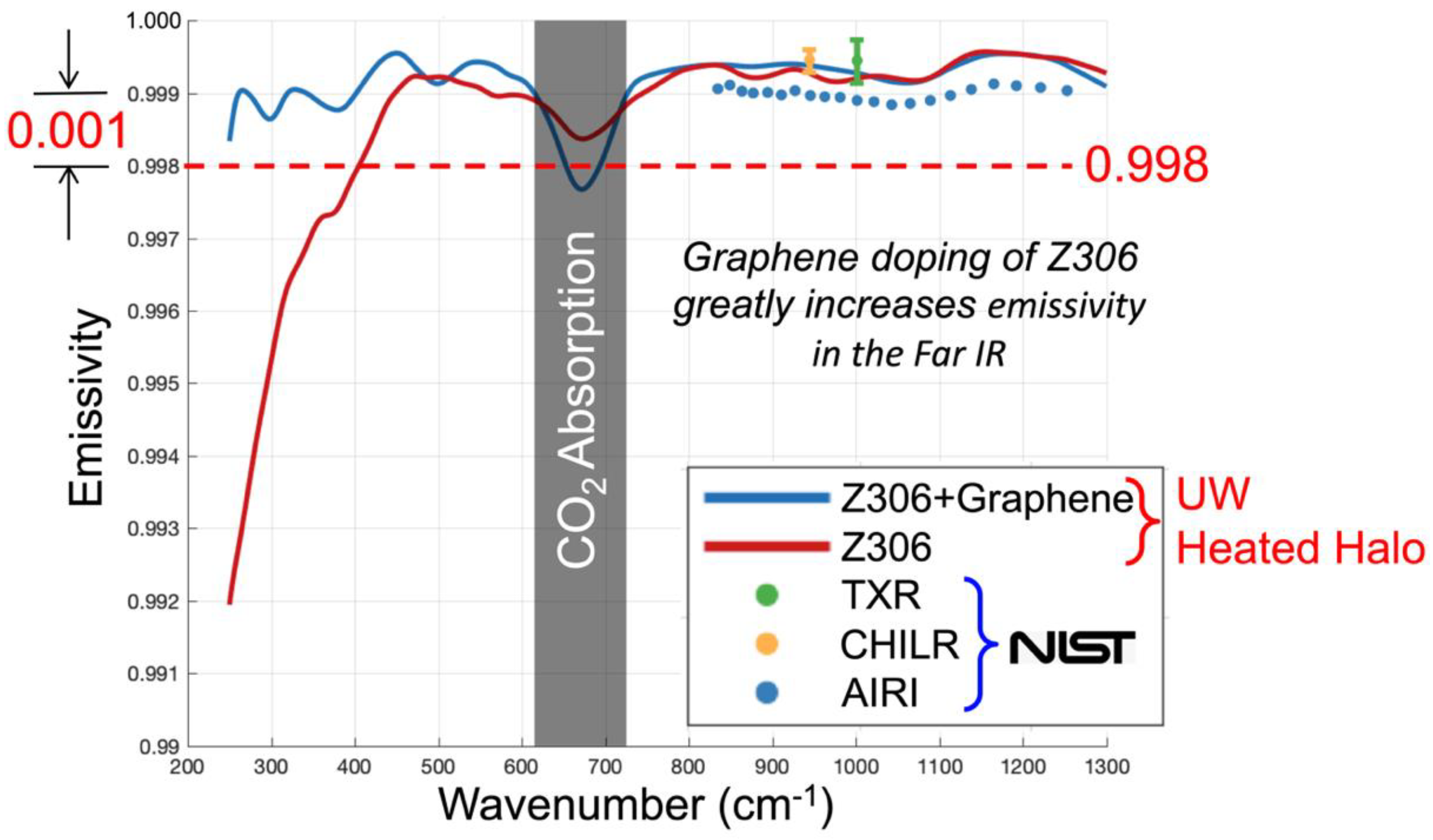
• The Calibrated Fourier Transform Spectrometer (CFTS) portion of ARI makes use of proven space-based type components (4 port, cube-corner interferometer; high emissivity calibration blackbody with emissivity greater than 0.998 out to 50 microns; all reflective fore-optics with stops carefully designed for radiometric accuracy; traditional detectors and small mechanical cooler combined to achieve contiguous spectral coverage from 200–2000 cm⁻¹ for climate products and to 2600 cm⁻¹ for additional intercalibration capability) to achieve highly accurate (better than 0.1 K 3-σ brightness temperature at scene temperature) spectral radiances at 0.625 cm⁻¹ resolution. Accuracy improvements over traditional sounding instruments (an order of magnitude at cold temperatures and at least a factor of 3 for warm temperatures) are achieved through the use of highly linear detectors, essentially eliminating polarization related measurement artifacts, and careful attention to minimizing blackbody temperature uncertainty. These are made possible by long-term climate trend observing requirements that do not demand low noise performance, high spatial resolution, or cross-track sampling. In fact, a relatively large spatial footprint (25–100 km) is advantageous for the intercalibration of other infrared instruments.
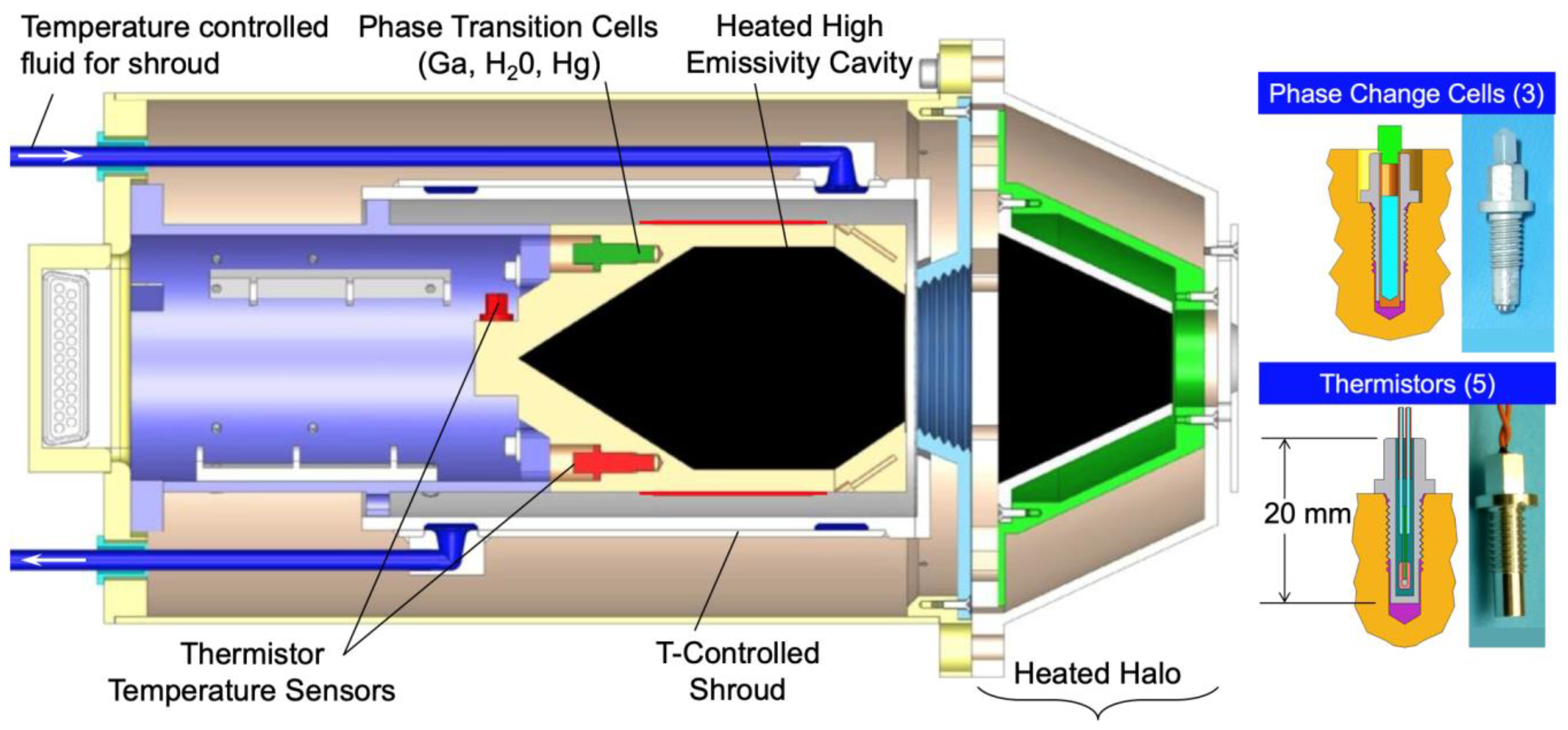
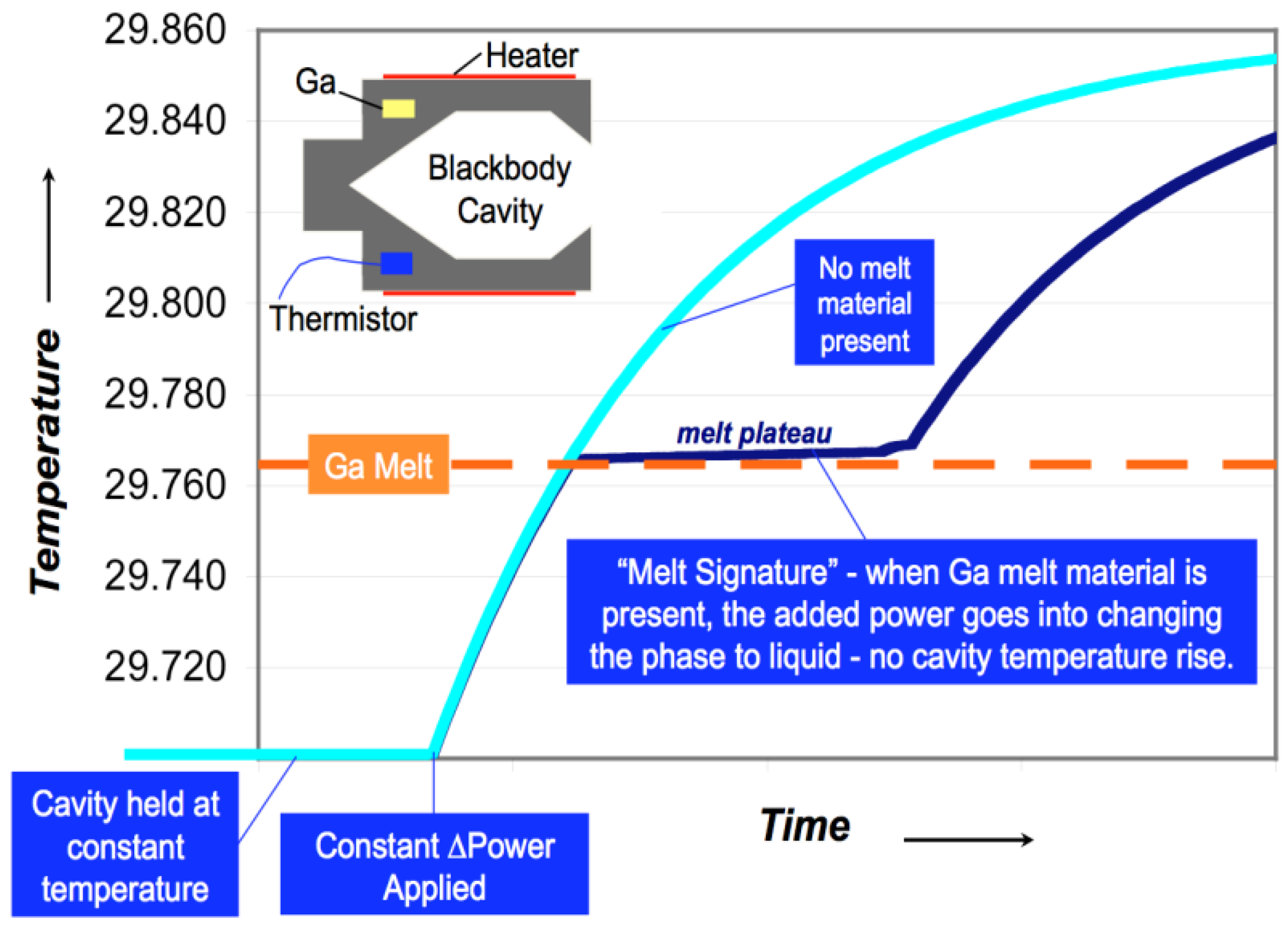
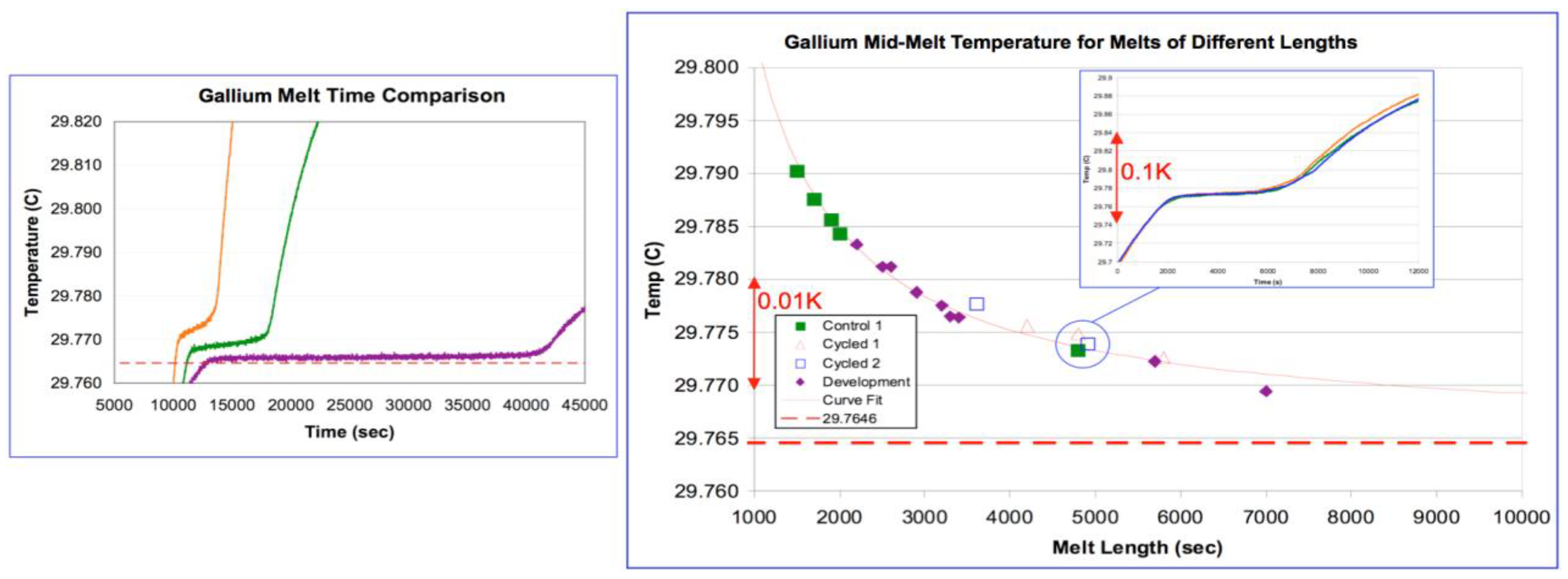
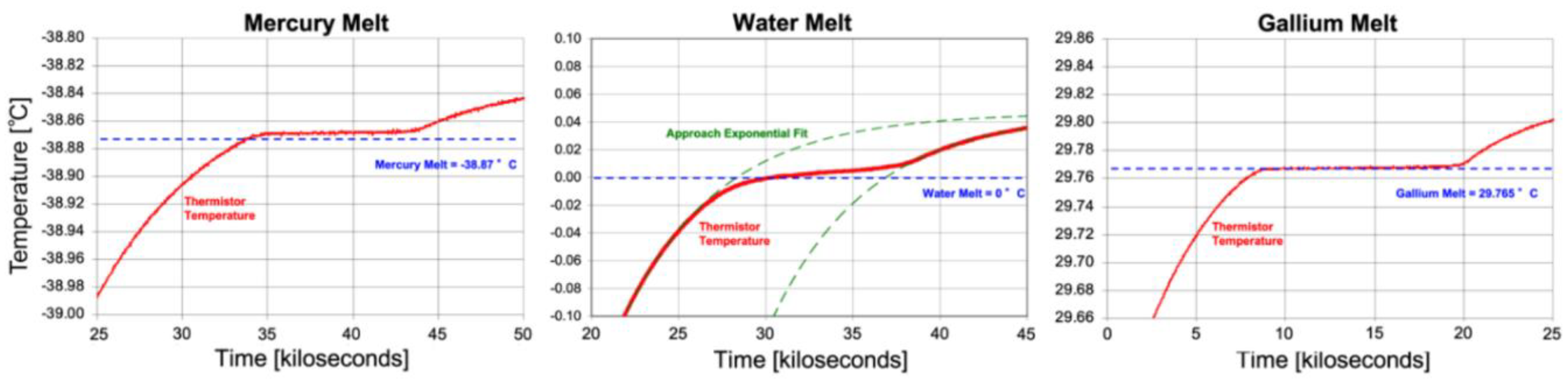
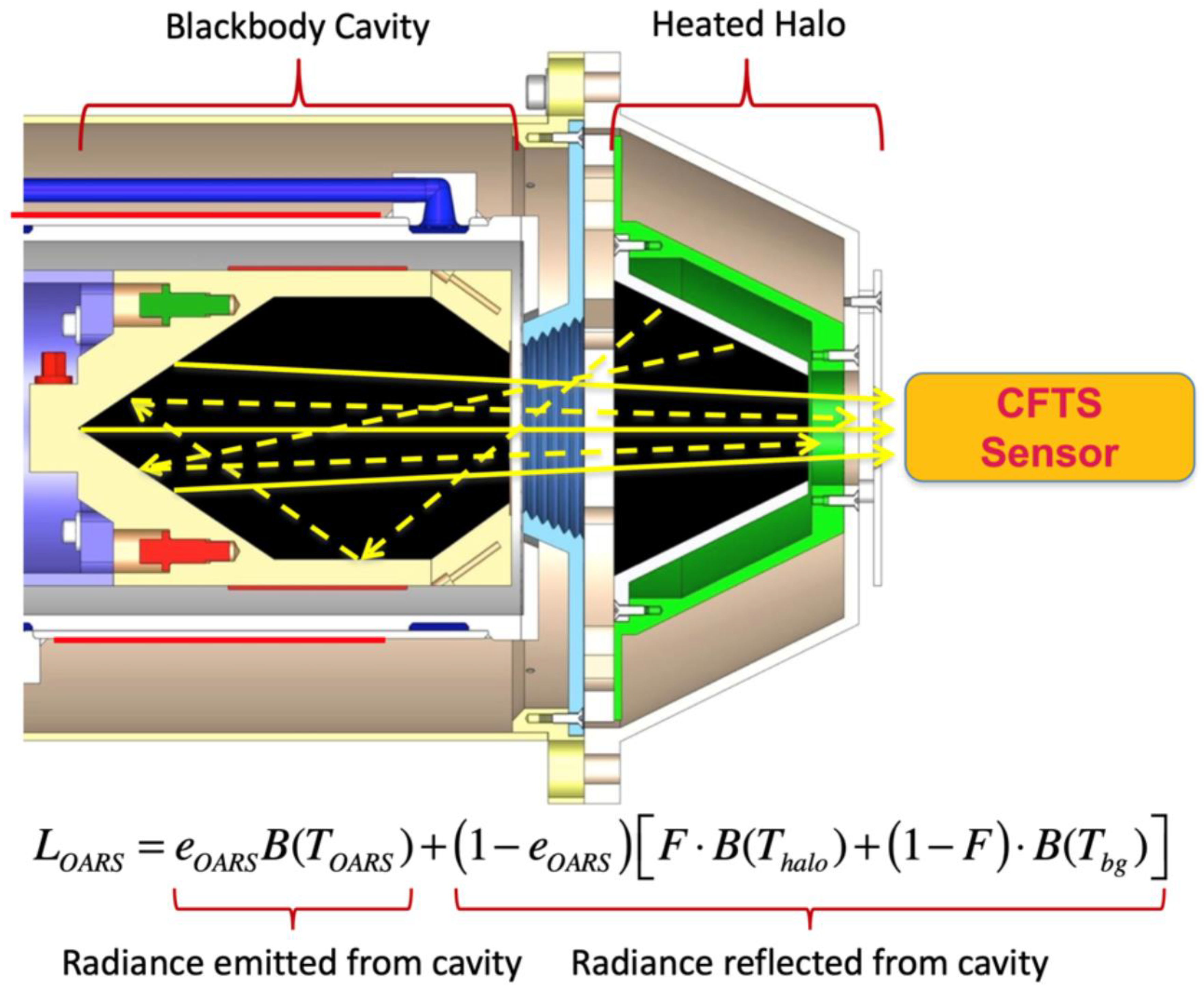
• The On-orbit Verification and Test (OVTS) portion of ARI allows the accuracy of the CFTS to be proven real time (or even improved if necessary). This is the fundamentally new thing about the ARI that allows it to offer a new climate benchmarking capability. When viewed with the interferometer of the CFTS, the new technologies of the OVTS provide observations for verification and test that are similar to those normally collected during carefully designed, pre-launch thermal vacuum testing. An On-orbit Absolute Radiance Standard (OARS) is provided to verify radiometric accuracy over a wide range of emitting temperatures. The fundamental SI temperature scale of the OARS blackbody is established and verified monthly by three miniature melt cells containing, gallium, water, and mercury, probably the most important new technology. The other fundamental property of a blackbody, its emissivity, is verified by another new space-based technology called the heated halo. Several other new testing capabilities, including accurate measurement of the spectral Instrument Line Shape, are included to make sure that the on-orbit radiometric and spectral uncertainty remains well-characterized, thereby avoiding false climate signatures.
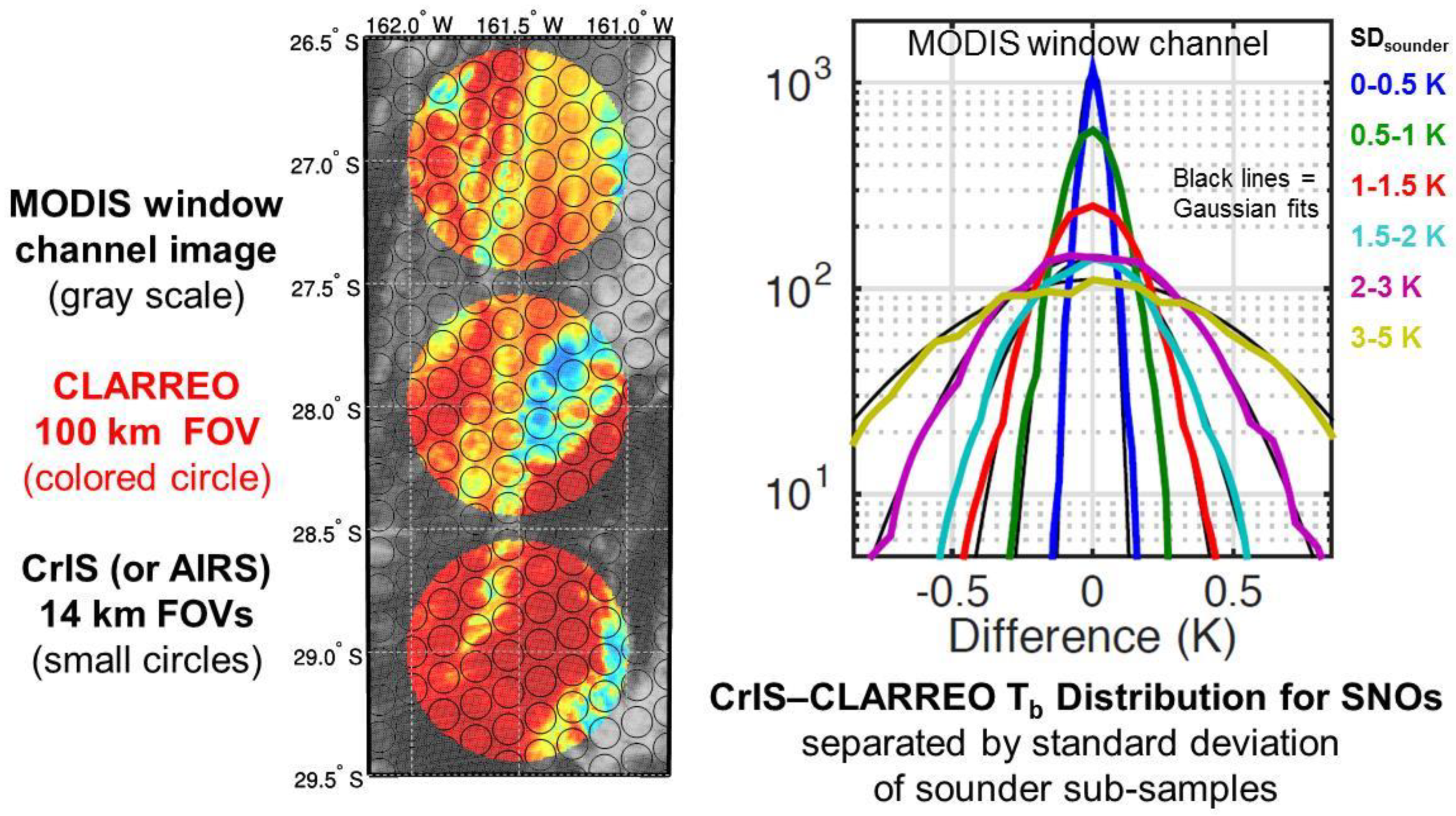
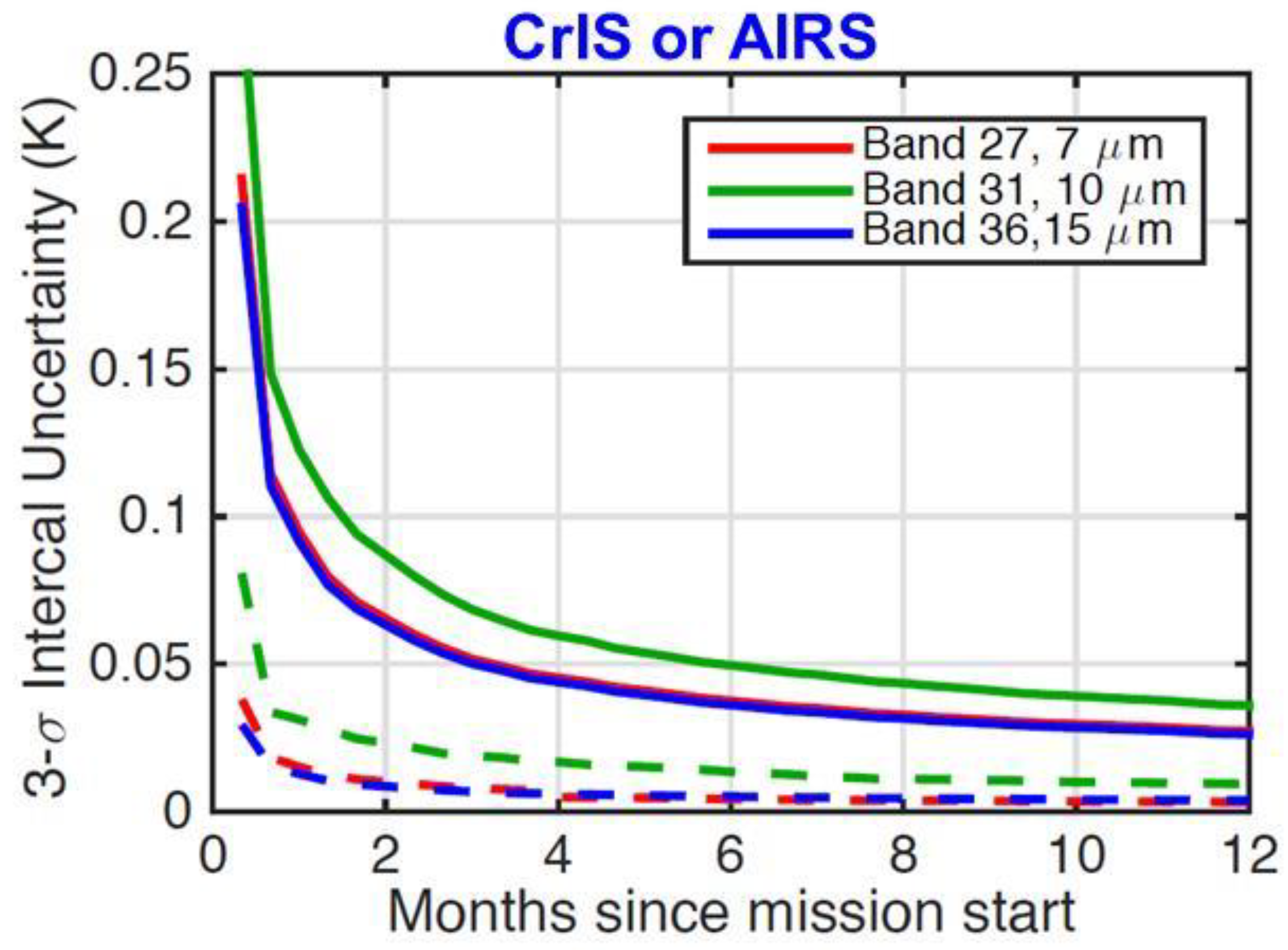
• It will be possible to transfer the highly accurate ARI calibration to other well-characterized infrared instruments on orbit. This property is very important for being able to achieve the unbiased temporal and spatial sampling required to establish a climate benchmark. Instead of needing to fly a fleet of ARI instruments in different orbits, the current more affordable plan would be to use ARI to inter-calibrate the international fleet of high spectral resolution sounding instruments, including the US CrIS, the European IASI, and the Chinese HIRAS. Here, we describe simulations and the fundamental properties of inter-calibrations that prove this key capability to transfer the highly accurate calibration of ARI to other high spectral resolution infrared sounding instruments. This inter-calibration approach is far more practical than trying to incorporate the ARI on-orbit verification and test capabilities into future operational sounding instruments that are already quite complex; their design optimization requires looking at the Earth as much of the available time as possible
• A Pathfinder Mission that would fly ARI on a precessing orbit like that of the International Space Station or a non-precessing true polar orbit would offer many opportunities for inter-calibration of the international fleet of an infrared sounding instrument in sun-synchronous orbits. Given the observing capability from having a pair of CrIS instruments in 1330 orbits, a pair of IASI instruments in 0930 orbits and a HIRAS in the 0530 orbit (starting soon) the opportunity for excellent spatial and temporal sampling can be expected for at least the next two decades.

We feel that moving ahead with the flight of a pathfinder, SI-based, climate benchmark mission based on ARI should be considered an urgent priority by the world’s space agencies.

References

1. Hansen, J.E.; Rossow, W.B.; Fung, I. Long-Term Monitoring of Global Climate Forcings and Feedbacks; NASA-CP-3234; National Aeronautics and Space Administration: Washington, DC, USA, 1993.
2. Anderson, J.; Goody, R.; Keith, D. Arrhenius: A Small Satellite for Climate Research; Harvard University: Cambridge, MA, USA, 1996. [Google Scholar]
3. Kirk-Davidoff, D.B.; Goody, R.M.; Anderson, J.G. Analysis of sampling errors for climate monitoring satellites. J. Clim. 2005, 18, 810–822. [Google Scholar] [CrossRef] [Green Version]
4. Smith, W.L.; Revercomb, H.E.; Howell, H.B.; Woolf, H.M.; LaPorte, D.D. The High Resolution Interferometer Sounder (HIS). In Atmospheric Radiation: Progress and Prospects, Proceedings of the Beijing International Radiation Symposium, Beijing, China, 26–30 August 1986; Springer: Berlin, Germany, 1987; pp. 271–281. [Google Scholar]
5. Revercomb, H.E.; LaPorte, D.D.; Smith, W.L.; Buijs, H.; Murcray, D.G.; Murcrayr, F.J.; Sromovsky, L.A. High-altitude aircraft measurements of upwelling IR radiance: Prelude to FTIR from geosynchronous satellite. Microchim. Acta 1988, 95, 439–444. [Google Scholar] [CrossRef]
6. Revercomb, H.E.; Buijs, H.; Howell, H.B.; LaPorte, D.D.; Smith, W.L.; Sromovsky, L.A. Radiometric calibration of IR Fourier transform spectrometers: Solution to a problem with the High-Resolution Interferometer Sounder. Appl. Opt. 1988, 27, 3210–3218. [Google Scholar] [CrossRef] [PubMed]
7. Revercomb, H.; Buijs, H.; Howell, H.; Knuteson, R.; LaPorte, D.; Smith, W.; Sromovsky, L.; Woolf, H. Radiometric calibration of IR interferometers: Experience from the High-resolution Interferometer Sounder (HIS) aircraft instrument. RSRM 1989, 87, 89–102. [Google Scholar]
8. Goody, R.; Haskins, R. Calibration of radiances from space. J. Clim. 1998, 11, 754–758. [Google Scholar] [CrossRef]
9. Knuteson, R.; Revercomb, H.; Best, F.; Ciganovich, N.; Dedecker, R.; Dirkx, T.; Ellington, S.; Feltz, W.; Garcia, R.; Howell, H. Atmospheric emitted radiance interferometer. Part I: Instrument design. J. Atmos. Ocean. Technol. 2004, 21, 1763–1776. [Google Scholar] [CrossRef]
10. Knuteson, R.; Revercomb, H.; Best, F.; Ciganovich, N.; Dedecker, R.; Dirkx, T.; Ellington, S.; Feltz, W.; Garcia, R.; Howell, H. Atmospheric emitted radiance interferometer. Part II: Instrument performance. J. Atmos. Ocean. Technol. 2004, 21, 1777–1789. [Google Scholar] [CrossRef]
11. Revercomb, H.; Walden, V.; Tobin, D.; Anderson, J.; Best, F.; Ciganovich, N.; Dedecker, R.; Dirkx, T.; Ellington, S.; Garcia, R. Recent results from two new aircraft-based Fourier transform interferometers: The Scanning High-resolution Interferometer Sounder and the NPOESS Atmospheric Sounder Testbed Interferometer. In Proceedings of the 8th International Workshop on Atmospheric Science from Space Using Fourier Transform Spectrometry (ASSFTS), Toulouse, France, 16–18 November 1998; pp. 16–18. [Google Scholar]
12. Ohring, G.; Tansock, J.; Emery, W.; Butler, J.; Flynn, L.; Weng, F.; St Germain, K.; Wielicki, B.; Cao, C.; Goldberg, M.; et al. Achieving satellite instrument calibration for climate change. EOS Trans. Am. Geophys. Union 2007, 88, 136. [Google Scholar] [CrossRef]
13. National Research Council. Earth Science and Applications from Space: National Imperatives for the Next Decade and Beyond; National Academies Press: Washington, DC, USA, 2007. [Google Scholar]
14. Smith, W.L.; Weisz, E.; Knuteson, R.; Revercomb, H.; Feldman, D. Retrieving Decadal Climate Change from Satellite Radiance Observations—A 100-year CO2 Doubling OSSE Demonstration. Sensors 2020, 20, 1247. [Google Scholar] [CrossRef] [Green Version]
15. Wielicki, B.; Young, D.F.; Mlynczak, M.G.; Thome, K.J.; Leroy, S.; Corliss, J.; Anderson, J.G.; Ao, C.O.; Bantges, R.; Best, F.; et al. Achieving Climate Change Absolute Accuracy in Orbit. Bull. Am. Meteorol. Soc. 2013, 94, 1519–1539. [Google Scholar] [CrossRef] [Green Version]
16. Liu, X.; Wu, W.; Wielicki, B.A.; Yang, Q.; Kizer, S.H.; Huang, X.; Chen, X.; Kato, S.; Shea, Y.; Mlynczak, M. Spectrally Dependent CLARREO Infrared Spectrometer Calibration Requirement for Climate Change Detection. J. Clim. 2017, 30, 3979–3998. [Google Scholar] [CrossRef]
17. Tobin, D.; Holz, R.; Nagle, F.; Revercomb, H. Characterization of the Climate Absolute Radiance and Refractivity Observatory (CLARREO) ability to serve as an infrared satellite intercalibration reference. J. Geophys. Res. Atmos. 2016, 121, 4258–4271. [Google Scholar] [CrossRef] [Green Version]
18. Tobin, D.; Revercomb, H.; Knuteson, R.; Taylor, J.; Best, F.; Borg, L.; DeSlover, D.; Martin, G.; Buijs, H.; Esplin, M.; et al. Suomi-NPP CrIS radiometric calibration uncertainty. J. Geophys. Res. Atmos. 2013, 118, 10589–510600. [Google Scholar] [CrossRef]
19. Eyre, J. Observation bias correction schemes in data assimilation systems: A theoretical study of some of their properties. Q. J. R. Meteorol. Soc. 2016, 142, 2284–2291. [Google Scholar] [CrossRef]
20. Best, F.A.; Adler, D.P.; Ellington, S.D.; Thielman, D.J.; Revercomb, H.E. On-orbit absolute calibration of temperature with application to the CLARREO mission. In Earth Observing Systems XIII; SPIE: Bellingham, WA, USA, 2008; Volume 7081, p. 70810O. [Google Scholar]
21. Best, F.A.; Adler, D.P.; Pettersen, C.; Revercomb, H.E.; Gero, P.J.; Taylor, J.K.; Knuteson, R.O. Results from recent vacuum testing of an on-orbit absolute radiance standard intended for the next generation of infrared remote sensing instruments. In Multispectral, Hyperspectral, and Ultraspectral Remote Sensing Technology, Techniques and Applications; SPIE: Bellingham, WA, USA, 2014; Volume: 9263, p. 926314. [Google Scholar]
22. Best, F.A.; Adler, D.P.; Pettersen, C.; Revercomb, H.E.; Gero, P.J.; Taylor, J.K.; Knuteson, R.O.; Perepezko, J.H. On-Orbit Absolute Radiance Standard for the Next Generation of IR Remote Sensing Instruments. In Multispectral, Hyperspectral, and Ultraspectral Remote Sensing Technology, Techniques and Applications; SPIE: Bellingham, WA, USA, 2012; Volume 8527, p. 85270N. [Google Scholar]
23. Best, F.A.; Adler, D.P.; Pettersen, C.; Revercomb, H.E.; Perepezko, J.H. On-orbit absolute temperature calibration using multiple phase change materials: Overview of recent technology advancements. In Multispectral, Hyperspectral, and Ultraspectral Remote Sensing Technology, Techniques, and Applications; SPIE: Bellingham, WA, USA, 2010; Volume 7857, p. 78570J. [Google Scholar]
24. Gero, P.J.; Dykema, J.A.; Anderson, J.G. A Quantum Cascade Laser–Based Reflectometer for On-Orbit Blackbody Cavity Monitoring. J. Atmos. Ocean. Technol. 2009, 26, 1596–1604. [Google Scholar] [CrossRef]
25. Gero, P.J.; Taylor, J.K.; Best, F.; Revercomb, H.; Knuteson, R.; Tobin, D.; Adler, D.P.; Ciganovich, N.; Dutcher, S.; Garcia, R. On-orbit Absolute Blackbody Emissivity Determination Using the Heated Halo Method. In Proceedings of the Fourier Transform Spectroscopy, Toronto, ON, Canada, 7 October 2011; p. FMA3. [Google Scholar]
26. Gero, P.J.; Taylor, J.K.; Best, F.A.; Garcia, R.K.; Revercomb, H.E. On-orbit absolute blackbody emissivity determination using the heated halo method. Metrologia 2012, 49, S1. [Google Scholar] [CrossRef]
27. Gero, P.J.; Taylor, J.K.; Best, F.A.; Revercomb, H.E.; Garcia, R.K.; Knuteson, R.O.; Tobin, D.C.; Adler, D.P.; Ciganovich, N.N. The heated halo for space-based blackbody emissivity measurement. In Multispectral, Hyperspectral, and Ultraspectral Remote Sensing Technology, Techniques and Applications IV; SPIE: Bellingham, WA, USA, 2018; p. 85270O. [Google Scholar]
28. Gero, P.J.; Taylor, J.K.; Best, F.A.; Revercomb, H.E.; Knuteson, R.O.; Tobin, D.C.; Adler, D.P.; Ciganovich, N.N.; Dutcher, S.; Garcia, R.K. On-orbit Absolute Blackbody Emissivity Determination Using the Heated Halo Method. In Multispectral, Hyperspectral, and Ultraspectral Remote Sensing Technology, Techniques and Applications III; SPIE: Bellingham, WA, USA, 2010; Volume 7857, p. 78570L. [Google Scholar]
29. Anderson, J.G.; Dykema, J.A.; Goody, R.; Hu, H.; Kirk-Davidoff, D. Absolute, spectrally-resolved, thermal radiance: A benchmark for climate monitoring from space. J. Quant. Spectrosc. Radiat. Transf. 2004, 85, 367–383. [Google Scholar] [CrossRef]
30. BIPM; IEC; IFCC; ISO; IUPAC; IUPAP; OIML. Guide to the Expression of Uncertainty in Measurement; SASO: Riyadh, Saudi Arabia, 1995; pp. 67–92. [Google Scholar]
31. BIPM; IEC; IFCC; IUPAC; ISO. The International Vocabulary of Metrology—Basic and general concepts and associated terms (VIM). JCGM 2012, 200, 2012. [Google Scholar]
32. Taylor, B.N.; Kuyatt, C.E. Guidelines for Evaluating and Expressing the Uncertainty of NIST Measurement Results; NIST Technical Note 1297; National Institute of Standards and Technology: Gaithersburg, MD, USA, 1994.
33. Taylor, J.K. Achieving 0.1 K Absolute Calibration Accuracy for High Spectral Resolution Infrared and Far Infrared Climate Benchmark Measurements; Université Laval: Quebec City, QC, Canada, 2014. [Google Scholar]
34. Reine, M.B. Nonlinear Response of 8–12 μm (HgCd)Te Photoconductor to Large Signal Photon Flux Levels; Morse, P.G., Ed.; Honeywell: Charlotte, NC, USA, 1979. [Google Scholar]
35. Revercomb, H.; Best, F.; Dedecker, R.; Dirkx, T.; Herbsleb, R.; Knuteson, R.; Short, J.; Smith, W. Atmospheric emitted radiance interferometer (AERI) for ARM. In Proceedings of the Fourth Symposium on Global Change Studies, Anaheim, CA, USA, 17 January 1993; pp. 46–49. [Google Scholar]
36. Revercomb, H.E. Techniques for Avoiding Phase and Non-linearity Errors in Radiometric Calibration: A Review of Experience with the Airborne HIS and Ground-based AERI. In Proceedings of the 5th International Workshop on Atmospheric Science from Space Using FTS, Madison, WI, USA, 30 November–2 December 1994; pp. 353–378. [Google Scholar]
37. Tobin, D.C. NAST-I Detector Nonlinearity Characterization. In Proceedings of the AIRS Science Team Meeting, Santa Barbara, CA, USA, 25–27 Febuary 2003. [Google Scholar]
38. Taylor, J.K.; Tobin, D.C.; Revercomb, H.E.; Knuteson, R.O.; Borg, L.; Best, F.A. Analysis of the CrIS Flight Model 1 Radiometric Linearity. In Proceedings of the Fourier Transform Spectroscopy, Beijing, China, 4 August 2009. [Google Scholar]
39. Knuteson, R.O.; Tobin, D.C.; Revercomb, H.E.; Taylor, J.K.; DeSlover, D.; Borg, L. Suomi NPP/JPSS Cross-Track Infrared Sounder (CrIS): Non-Linearity Assessment And On-Orbit Monitoring. In Proceedings of the 93rd AMS Annual Meeting, Austin, TX, USA, 24 December 2012. [Google Scholar]
40. Best, F.A.; Revercomb, H.E.; Knuteson, R.O.; Tobin, D.C.; Thielman, D.; Ellington, S.; Werner, M.; Adler, D.; Taylor, J.K.; Smith, W.L.; et al. GIFTS On-board Blackbody Calibration Subsystem. In Proceedings of the NASA GIFTS EDU and Other FTS Instruments, San Diego, CA, USA, 11 January 2006. [Google Scholar]
41. Best, F.A.; Revercomb, H.E.; Tobin, D.C.; Knuteson, R.O.; Taylor, J.K.; Thielman, D.J.; Adler, D.P.; Werner, M.W.; Ellington, S.D.; Elwell, J.D.; et al. Performance verification of the Geosynchronous Imaging Fourier Transform Spectrometer (GIFTS) on-board blackbody calibration system. In Multispectral, Hyperspectral, and Ultraspectral Remote Sensing Technology, Techniques, and Applications; SPIE: Bellingham, WA, USA, 2006; Volume 6405, p. 64050I. [Google Scholar]
42. Siwek, W.; Sapoff, M.; Goldberg, A.; Johnson, H.; Botting, M.; Lonsdorf, R.; Weber, S. Stability of NTC thermistors. Temp. Meas. Control. Sci. Ind. 1992, 6, 497–502. [Google Scholar]
43. Best, F.; Revercomb, H.; Knuteson, R.; Tobin, D.; Dedecker, R.; Dirkx, T.; Mulligan, M.; Ciganovich, N.; Te, Y. Traceability of absolute radiometric calibration for the Atmospheric Emitted Radiance Interferometer (AERI). In Proceedings of the 2003 Conference on Characterization and Radiometric Calibration for Remote Sensing, San Diego, CA, USA, 10 November 2003. [Google Scholar]
44. Best, F.A. Accurately Calibrated Airborne and Ground-Based Fourier Transform. Spectrometers II: HIS and AERI Calibration Techniques, Traceability, and Testing; University of Wisconsin: Madison, WI, USA, 1997. [Google Scholar]
45. Turner, D.; Knuteson, R.; Revercomb, H.; Dedecker, R.; Feltz, W. An Evaluation of the Nonlinearity Correction Applied to Atmospheric Emitted Radiance Interferometer (AERI) Data Collected by the Atmospheric Radiation Measurement Program; DOE ARM Climate Research Facility: Washington, DC, USA, 2004.
46. Revercomb, H.; Best, F. Calibration of the Scanning High-resolution Interferometer Sounder (SHIS) Infrared Spectrometer: Overview (Parts 1 and 2). In Proceedings of the 2005 Calcon Workshop, Calibration of Airborne Sensor Systems, Vienna, Austria, 29–30 August 2005. [Google Scholar]
47. Revercomb, H.E.; Knuteson, R.O.; Best, F.A.; Tobin, D.C.; Smith, W.L.; LaPorte, D.D.; Ellington, S.D.; Werner, M.W.; Dedecker, R.G.; Garcia, R.K. Scanning high-resolution interferometer sounder (S-HIS) aircraft instrument and validation of the Atmospheric InfraRed Sounder (AIRS). In Proceedings of the Optical Remote Sensing, Yalta, Ukraine, 20 September–4 October 2003; p. JMA4. [Google Scholar]
48. Revercomb, H.E.; Tobin, D.C.; Knuteson, R.O.; Best, F.A.; Smith, W.; LaPorte, D.; Ellington, S.; Werner, M.; Garcia, R.; Ciganovich, N. Highly accurate FTIR observations from the scanning HIS aircraft instrument. In Proceedings of the SPIE, Denver, CO, USA, 4 November 2004; pp. 41–53. [Google Scholar]
49. Taylor, J.; Best, F.; Ciganovich, N.; Dutcher, S.; Ellington, S.; Garcia, R.; Howell, H.; Knuteson, R.; LaPorte, D.; Nasiri, S. Performance of an infrared sounder on several airborne platforms: The scanning high resolution interferometer sounder (S-HIS). In Proceedings of the Earth Observing Systems X, San Diego, CA, USA, 1 June 2009; p. 588214. [Google Scholar]
50. Taylor, J.K.; Revercomb, H.E.; Best, F.A.; Tobin, D.C.; Knuteson, R.O. GIFTS EDU Radiometric Calibration Performance Assessment. In Proceedings of the NASA GIFTS EDU and Other FTS Instruments, Hampton, VA, USA, 30 October 2006. [Google Scholar]
51. Taylor, J.K.; Tobin, D.C.; Revercomb, H.E.; Knuteson, R.O.; Borg, L.; Best, F.A. Analysis of CrIS Flight Model 1 Radiometric Linearity and Radiometric Uncertainty. In ASSFTS 14; Optical Society of America: Washington, DC, USA, 2009. [Google Scholar]
52. Taylor, J.K.; Tobin, D.C.; Revercomb, H.E.; Knuteson, R.O.; Borg, L.; Best, F.A. Analysis of the CrIS Flight Model 1 Radiometric Linearity. In Proceedings of the Fourier Transform Spectroscopy, Baltimore, MD, USA, 14 May 2012. [Google Scholar]
53. Rowe, P.M.; Neshyba, S.P.; Cox, C.J.; Walden, V.P. A responsivity-based criterion for accurate calibration of FTIR emission spectra: Identification of in-band low-responsivity wavenumbers. Optics Express 2011, 19, 5930–5941. [Google Scholar] [CrossRef]
54. Rowe, P.M.; Neshyba, S.P.; Walden, V.P. Responsivity-based criterion for accurate calibration of FTIR emission spectra: Theoretical development and bandwidth estimation. Optics Express 2011, 19, 5451–5463. [Google Scholar] [CrossRef] [PubMed] [Green Version]
55. Best, F.A.; Revercomb, H.E.; Knuteson, R.O.; Tobin, D.C.; Ellington, S.D.; Werner, M.W.; Adler, D.P.; Garcia, R.K.; Taylor, J.K.; Ciganovich, N.N. The Geosynchronous Imaging Fourier Transform Spectrometer (GIFTS) on-board blackbody calibration system. In Proceedings of the Fourth International Asia-Pacific Environmental Remote Sensing Symposium 2004: Remote Sensing of the Atmosphere, Ocean, Environment, and Space, Honolulu, HI, USA, 30 December 2004; pp. 77–87. [Google Scholar]
56. Best, F.A.; Knuteson, R.O.; Revercomb, H.E.; Tobin, D.C.; Gero, P.J.; Taylor, J.K.; Rice, J.P.; Hanssen, L.; Mekhontsev, S. Measurements of the Atmospheric Emitted Radiance Interferometer (AERI) blackbody emissivity and radiance using multiple techniques. In Proceedings of the CALCON Technical Conference, Logan, UT, USA, 22 January 2010. [Google Scholar]
57. Rice, J.P.; Johnson, B.C. The NIST EOS thermal-infrared transfer radiometer. Metrologia 1998, 35, 505. [Google Scholar] [CrossRef]
58. Zeng, J.; Hanssen, L. An infrared laser-based reflectometer for low reflectance measurements of samples and cavity structures. In Reflection, Scattering, and Diffraction from Surfaces; SPIE: Bellingham, WA, USA, 2008; p. 70650F. [Google Scholar]
59. Mekhontsev, S.; Khromchenko, V.; Hanssen, L.M. NIST radiance temperature and infrared spectral radiance scales at near-ambient temperatures. Int. J. Thermophys. 2008, 29, 1026–1040. [Google Scholar] [CrossRef]
60. Dykema, J.A.; Witinski, M.; Anderson, J. Quantum Cascade Laser based reflectometry for on-orbit blackbody emissivity measurements for CLARREO. In Proceedings of the CALCON Technical Conference, Logan, UT, USA, 22 January 2010. [Google Scholar]
61. Dowell, M.; Lecomte, P.; Husband, R.; Schulz, J.; Mohr, T.; Tahara, Y.; Eckman, R.; Lindstrom, E.; Wooldridge, C.; Hilding, S.; et al. Strategy towards an Architecture for Climate Monitoring from Space; CEOS: Washington, DC, USA, 2013. [Google Scholar]
62. Goldberg, M.; Ohring, G.; Butler, J.; Cao, C.; Datla, R.; Doelling, D.; Gärtner, V.; Hewison, T.; Iacovazzi, B.; Kim, D. The global space-based inter-calibration system. Bull. Am. Meteorol. Soc. 2011, 92, 467–475. [Google Scholar] [CrossRef]
63. Hewison, T. Extending the Global Space-based Inter-Calibration System (GSICS) to tie Satellite Radiances to an Absolute Scale. Remote Sensing 2020, 12, 1782. [Google Scholar] [CrossRef]
64. Revercomb, H.; Best, F.; Tobin, D.; Knuteson, B.; Smith, N.; Smith Sr, W.L.; Weisz, E. Monitoring climate from space: A metrology perspective. In Earth Observing Missions and Sensors: Development, Implementation, and Characterization IV; SPIE: Bellingham, WA, USA, 2016; p. 98810F. [Google Scholar]
Figure 1. Radiometric uncertainty (RU) of the three spectral bands of the SNPP Cross-track Infrared Sounder (CrIS) operational sounder compared to that for ARI. The format of this figure follows that of Tobin et al. [18]. The RU is assessed via perturbation of the calibration equation, following accepted metrology approaches, as described in Section 4.2 and by Tobin et al. [18]. The colors represent the density of occurrence in a typical Earth atmosphere for the CrIS RU. The lower bound for CrIS is set by uncertainty in the radiance of its internal calibration target (ICT). Larger longwave (LW) band (shortwave (SW) band) uncertainties arise from residual non-linearity (polarization) correction uncertainty, while the midwave (MW) band values are a combination of both mechanisms. The ARI calibration uncertainty, shown in black, is totally dominated by the uncertainty of the radiance from its internal calibration target resulting in an order of magnitude reduction in peak uncertainties at cold temperatures. Additionally, the ARI On-orbit Absolute Radiance Standard (OARS, see Section 5) provides end-to-end calibration verification with direct on-orbit traceability to absolute standards.
Remotesensing 12 01915 g001
Figure 2. A notional illustration indicating the primary Absolute Radiance Interferometer subsystems and optical path.
Remotesensing 12 01915 g002
Figure 3. (a) Front view of the completed ARI sensor prototype, showing the Ambient Blackbody (ABB) calibration reference, the Hot Blackbody (HBB) calibration reference, and the On-orbit Absolute Radiance Standard (OARS) calibration verification blackbody; any of these sources can be selected using the scene selection mirror (SSM). The OARS includes the Heated Halo On-orbit Cavity Emissivity Monitor (OCEM), which is located inside the OARS case and not visible here. (b) Internal view of the completed ARI sensor prototype. Primary components are labeled and include the ABB Generic Interferometer for Climate Studies (GICS), the Stirling cooler, the fore-optics, far-infrared (FIR) aft-optics and deuterated triglycine sulfate (DTGS) detector, the infrared (IR) aft-optics and detector dewar module, and the second input port reference source.
Remotesensing 12 01915 g003
Figure 4. The ABB Generic Interferometer for Climate Studies (GICS) shown here during post-delivery testing at the University of Wisconsin-Madison Space Science and Engineering Center (UW-SSEC) was selected for the ARI interferometer core.
Remotesensing 12 01915 g004
Figure 5. Predicted on-orbit radiometric calibration uncertainty (dashed) and calibration verification source uncertainty (solid) (k = 3).
Remotesensing 12 01915 g005
Figure 6. Predicted on-orbit combined radiometric calibration and verification uncertainty (k = 3).
Remotesensing 12 01915 g006
Figure 7. Predicted laboratory radiometric calibration uncertainty (dashed) and calibration verification source uncertainty (solid) (k = 3).
Remotesensing 12 01915 g007
Figure 8. Predicted laboratory combined radiometric calibration and verification uncertainty (k = 3).
Remotesensing 12 01915 g008
Figure 9. Predicted vacuum radiometric calibration uncertainty (dashed) and calibration verification source uncertainty (solid) (k = 3).
Remotesensing 12 01915 g009
Figure 10. Predicted vacuum combined radiometric calibration and verification uncertainty (k = 3).
Remotesensing 12 01915 g010
Figure 11. Radiance summary for the ARI DTGS detector calibration verification conducted under vacuum. The OARS was operated over a range of temperatures from approximately 216 K to 334 K.
Remotesensing 12 01915 g011
Figure 12. ARI calibration verification results for tests conducted under vacuum. Observed brightness temperature for the DTGS detector is shown in red and the black dashed line indicates predicted brightness OARS brightness temperature. The noise for the DTGS detector in the ARI prototype demonstration is significantly larger than what is expected for the flight design. Note that the brightness temperature of a real blackbody depends on both the blackbody temperature and emissivity, and for a non-ideal blackbody the brightness temperature will not be spectrally flat due to the spectral dependence of the emissivity.
Remotesensing 12 01915 g012
Figure 13. DTGS detector brightness temperature residuals (observed–predicted) for end-to-end calibration verification datasets conducted under vacuum. The results have been spectrally averaged in 50 cm−1 wide bins for noise reduction. Error bars represent statistical error only (k = 1 standard error). Total (calibration and calibration verification) radiometric uncertainty (k = 3) is shown in blue, and the grey dashed lines indicate ±0.1 K. The effect of low SNR is evident at the edges of the spectral band.
Remotesensing 12 01915 g013
Figure 14. ARI calibration verification results for tests conducted under vacuum. Observed brightness temperature for the long-wave Mercury-Cadmium-Telluride (HgCdTe or MCT) detector is shown in green and the black dashed line indicates predicted brightness OARS brightness temperature.
Remotesensing 12 01915 g014
Figure 15. Long-wave MCT detector brightness temperature residuals (observed–predicted) for end-to-end calibration verification datasets conducted under vacuum. The results have been spectrally averaged in 25 cm−1 wide bins for noise reduction. Error bars represent statistical error only (k = 1 standard error). Total (calibration and calibration verification) radiometric uncertainty (k = 3) is shown in blue, and the grey dashed lines indicate ±0.1 K. The artifact associated with the original field stop is evident. The solution to this issue was implemented post-vacuum testing.
Remotesensing 12 01915 g015
Figure 16. ARI calibration verification in the laboratory conditions under dry air purge, following the resolution of the fore-optics stray-light issue discovered during vacuum testing. Observed–predicted OARS brightness temperature residuals for the (a) DTGS detector (averaged over 50 cm−1 for noise reduction) and (b) the MCT (averaged over 5 cm−1 for noise reduction). The differences generally fall inside the ±0.1 K boundaries shown, and the improvement for both bands compared to vacuum tests is evident. In the far-infrared from 200–300 cm−1 the low signal to noise due to the less than optimum beamsplitter coating causes a small bias. Total (calibration and calibration verification) radiometric uncertainty (k = 3) for the laboratory environment is shown in blue, and the grey dashed lines indicate ±0.1 K. Error bars represent statistical error only (k = 1 standard error). The predicted radiances for the OARS do not include atmospheric absorption calculations and as a result, the 15 μm CO2 band absorption signature (shaded in grey) is evident in the residual.
Remotesensing 12 01915 g016
Figure 17. Section view schematic of the OARS showing the blackbody cavity and the embedded thermistor temperature sensors and phase transition cells, which are broken out in more detail at right. Multilayer insulation is not shown.
Remotesensing 12 01915 g017
Figure 18. The sequence of events during a typical melt of gallium confined in a phase transition cell and imbedded into an OARS as illustrated in Figure 17. After initial stabilization in the constant temperature mode, a constant power is used to transition through the melt plateau.
Remotesensing 12 01915 g018
Figure 19. The plot on the left shows three different melts of different duration. The longer the melt the closer the plateau approaches the theoretical melt temperature (indicated with a dashed red line). The large plot at right illustrates this by plotting mid-melt temperature vs. melt length—each data point corresponds to a single melt. The inset plot at upper right shows the three melt signatures associated with the circled data points, indicating great reproducibility.
Remotesensing 12 01915 g019
Figure 20. Melts of mercury, water, and gallium obtained using the ARI Prototype OARS. Each melt temperature is established to within 10 mK (k = 3), half of a division in each of the plots above.
Remotesensing 12 01915 g020
Figure 21. OARS temperature gradients at −20 °C and 24-h stability in a vacuum environment. The temperature of the ARI instrument and its surroundings is +20 °C. The red dashed lines in the diagram on the right represent the field of view of the Calibrated Fourier Transform Spectrometer (CFTS) as it observes the OARS.
Remotesensing 12 01915 g021
Figure 22. Illustration of the Heated Halo approach for measuring blackbody hemispheric-to-normal spectral emissivity on orbit.
Remotesensing 12 01915 g022
Figure 23. Laboratory emissivity measurements of the OARS cavity using the Heated Halo (red and blue solid curves), showing good agreement with three different independent NIST measurements. The uncertainty of the Heated Halo measurements is 0.06% (k = 3). TXR and CHILR uncertainties are as indicated at the discrete data points. The ARI uncertainty is expected to be less than 0.1% (k = 2). The CO2 absorption feature is due to operation in a laboratory environment and will not be present under vacuum conditions.
Remotesensing 12 01915 g023
Figure 24. The Quantum Cascade Laser (QCL) is injected to the center of the 45° Scene Mirror from the back of the optical system, allowing all targets to be illuminated in identical fashion, while being viewed by the Fourier Transform Spectrometer (FTS).
Remotesensing 12 01915 g024
Figure 25. ARI ILS measurement (left) and Ambient Blackbody reflectivity measurements obtained using the QCL (right). In the plot on the right, the blue curve is the measured radiance when the blackbody is illuminated with the QCL, the black curve is the radiance from the blackbody without QCL illumination, and the blue region is a measure of the laser power reflected from the blackbody.
Remotesensing 12 01915 g025
Figure 26. The concept of operations for the ARI instrument on-orbit, over a short-term period of 120 s, as shown at left, where the blue diamonds indicate the normal Earth/calibration views and the squares indicate specialized verification and test views. The wide range of OVTS views employed over a long-term period of 22 days is shown at right, where the red lines differentiate OVTS functions from the normal calibration cycle views shown in green.
Remotesensing 12 01915 g026
Figure 27. Illustration of the properties of the CLARREO intercalibration approach for comparison to operational sounding instruments. On the left, a black-and-white MODIS image is shown with the large CLARREO footprints color enhanced to illustrate individual Simultaneous Nadir Overpasses (SNOs). MODIS Band 32 brightness temperatures are shown with an RGB color scale with values ranging from 300 K (red) to 200 K (blue). The much smaller sounder footprints are overlaid as black circles. On the right, the key statistical properties of SNOs are shown, demonstrating that the distribution of radiance differences is composed of a summation of Gaussian distributions, each well characterized by the standard deviation of sounder sub-samples in the SNO.
Remotesensing 12 01915 g027
Figure 28. Simulated Intercalibration Uncertainty (IU) as a function of time since mission start for a single CLARREO polar orbit with 50 km IR footprints and 20 s between samples.
Remotesensing 12 01915 g028