Mapping Land Cover and Tree Canopy Cover in Zagros Forests of Iran: Application of Sentinel-2, Google Earth, and Field Data

Abstract

The Zagros forests in Western Iran are valuable ecosystems that have been seriously damaged by human interference (harvesting the wood and forest sub-products, converting the forests to the agricultural lands, and grazing) and natural events (drought events and fire). In this study, we generated accurate land cover (LC), and tree canopy cover percentage (TCC%) maps for the forests of Shirvan County, a part of Zagros forests in Western Iran using Sentinel-2, Google Earth, and field data for protective management. First, we assessed the accuracy of Google Earth data using 300 random field plots in 10 different land cover types. For land cover mapping, we evaluated the performance of four supervised classification algorithms (minimum distance (MD), Mahalanobis distance (MaD), neural network (NN), and support vector machine (SVM)). The accuracy of the land cover maps was assessed using a set of 150 stratified random plots in Google Earth. We mapped the forest canopy cover by using the normalized difference vegetation index (NDVI) map, and field plots. We calculated the Pearson correlation between the NDVI values and the TCC% (obtained from field plots). The linear regression between the NDVI values and the TCC% was used to obtain the predictive model of TCC% based on the NDVI. The results showed that Google Earth data yielded an overall accuracy of 94.4%. The SVM algorithm had the highest accuracy for the classification of Sentinel-2 data with an overall accuracy of 81.33% and a kappa index of 0.76. The results of the forest canopy cover analysis showed a Pearson correlation coefficient of 0.93 between the NDVI and TCC%, which is highly significant. The results also showed that the linear regression model is a good predictive model for TCC% estimation based on the NDVI (r² = 0.864). The results can be used as a baseline for decision-makers to monitor land cover change in the region, whether produced by human activities or natural events and to establish measures for protective management of forests.

1. Introduction

Iran is a vast country with different types of climate and vegetation, a wide range of elevation, and varied geological formations, the combination of which led to having rich biological diversity [1] and numerous endemic species [2]. The Zagros forests of Iran on Zagros Mountain extend from the northwest to the southwest of the country, making it the regional habitat with a large concentration of fauna and flora [2,3,4]. Although the Zagros Mountain is not the most bio-diverse region in Iran, the Zagros oak forests are one of the most important natural ecosystems in Iran, that are 5500 years old [5,6,7,8]. Besides, these forests have an essential role in soil and water conservation in the Zagros Mountains in western Iran [9]. Over the last 30 years, climate change, population growth, and the dependence of people’s livelihoods on these forests (by harvesting the wood and forest sub-products, converting forests to the agricultural lands, and grazing) have resulted in degradation of these natural ecosystems [9,10]. These forests, especially in Ilam Province in Western Iran, have been damaged by climate change, droughts (especially in oak forests), fires and human interference through, for example, the dependence of the residents on these areas for the provision of wood for fuel and land for livestock, agriculture, and grazing [9,10,11,12]. The biodiversity, ecosystem services, and economical production of the Zagros forests also suffered due to the lack of a management plan for these forests [12,13]. On the other hand, despite the high environmental value of these forests, there is not a comprehensive plan for the conservation of these forests on the national scale. Therefore, having accurate maps of the Zagros forests (area, density, and distribution) of Iran will be very useful in helping to detect the loss or gain process of these forests. Providing accurate maps of Zagros forests faciliates the effective management of these forests [14]. For example, providing a precise land cover map in Zagros forests would help the managers of the natural resources to find the answers to questions such as (1) how natural and human-made land covers are distributed in the Zagros forest, (2) how large the exact area of different land covers inside Zagros forests is, or (3) how human-made land covers interact with the natural land covers (forests and rangelands). Additionally, providing an accurate forest cover map including different density classes would guide the forest managers to analyze (1) where the Zagros forests are distributed, (2) how much the exact area of Zagros forests in western Iran is, or (3) how the forest cover is disaggregated in different density classes. Therefore, providing land cover and forest canopy cover maps in these forests will be the first step to protecting them and preventing further destruction [15].

Remote sensing data is an excellent source for mapping, monitoring, and understanding the land cover changes because of its synoptic, multi-spectral, and multi-temporal nature [14,15,16,17]. Satellite images have been widely applied for land use/land cover mapping in different areas around the world, such as in Brazil [18], India [19], and Turkey [20]. Landsat-8 and normalized difference vegetation index (NDVI) have been used to estimate the tree species diversity in the savannah woodland of southern Africa [21] and mapping the tree canopy cover (TCC) in the south of Ouagadougou in central Burkina Faso [22] and semi-arid forests of the Sahel [23]. At a coarser spatial resolution, the moderate resolution imaging spectroradiometer (MODIS) imagery allowed the land cover mapping in other countries such as India, Germany, and Pakistan [24,25,26]. IRS data was also used for land cover mapping in some regions around the world [27,28,29]. In recent years, Sentinel-2 satellite image data has proven very useful for land use/land cover mapping [30,31,32,33], achieving superior results for this purpose by applying the support vector machine (SVM) algorithm [30,33]. In the case of forest monitoring and management, Sentinel-2 images have successfully performed tree cover mapping [34], tree species mapping [35], vegetation mapping [36], forest type mapping [37], forest succession [38], forest decline [39], quantitative estimation of biophysical variables [40], and estimation of defoliation of needle-leaf stands [41]. The results of these studies have shown that the SVM algorithm has led to high accuracies for vegetation mapping and forest monitoring [36,41].

Regarding forest density and canopy cover mapping, vegetation indices have been widely used to estimate vegetation density or canopy cover mapping in forest areas. Pereira et al. [42] used Landsat TM imagery and fieldwork data to determine the canopy cover percentage in Mediterranean shrublands. They obtained the best results when using the NDVI to estimate the canopy cover percentage (r² = 0.65). Oliveira [43] used field radiometry and Landsat TM imagery to estimate several shrub parameters in the Alto-Dao region in Portugal. Field radiometry results showed that the NDVI was a vegetation index with high performance (r = 0.75). Calvao and Palmeirim [44] collected field data of Mediterranean shrublands and developed correlations between several biophysical parameters and spectral variables (single channel reflectance and NDVI) from Landsat TM data. The higher correlation for canopy cover was obtained with TM band 3 (r = −0.91) and NDVI (r = 0.91). Karlson et al. [22] used the NDVI from the WorldView-2 and Landsat-8 image to partition a woodland landscape in Burkina Faso into three classes based on the tree canopy cover density. Results showed that the dry-season NDVI and other spectral and textural characteristics were the most important factors in tree canopy cover mapping in the study area. Mohamed [23] mapped the tree canopy cover in the semi-arid Sahel using Landsat-8 and Google Earth imagery. The developed method utilized the NDVI as the predictor variable coupled with estimations of tree canopy cover from Google Earth imagery as the response variable. The results showed a strong correlation (r² = 0.83) between the NDVI derived from Landsat 8 imagery and the TCC estimations from Google Earth imagery. Soares et al. [45] mapped tree canopy cover changes in space and time in High Nature Value Farmland in southeast Portugal using aerial photography and Landsat images to prioritize reforestation efforts. The results showed that the dry-season NDVI was positively related to tree canopy cover changes, both across space and time. Barakat et al. [46] used a supervised classification algorithm on Landsat-8 and NDVI to quantify the extent and density change of forest covers, crops, and bare soils in Morocco. The overall classification accuracy was 97.76% and 95.80% in 2001 and 2015 images, respectively. He adopted a method of thresholding the NDVI [47] to highlight the density of each forest stand. Based on the NDVI values, the image was classified into three distinct thematic classes: NDVI < 0.1: without vegetation, 0.2 < NDVI < 0.4: slightly dense forest, and 0.4 < NDVI < 0.74: dense forest. The identification of the best-fitting threshold value was based on the comparison between the Google Earth images and the NDVI results. Chasmer et al. [48] used the NDVI, simple ratio (SR), and soil adjusted vegetation index (SAVI) derived from a SPOT5 satellite image to estimate canopy cover. Their results indicated that the NDVI and SAVI are more comparable to canopy cover than other vegetation indices.

The results of several studies mentioned above have demonstrated that NDVI is the best vegetation index for estimating the tree canopy cover in different forest areas around the world [22,23,40,42,43,44,45,46,47,48,49]. Besides, among different methods for predicting the relationship between TCC% and NDVI, linear regression has successfully been applied for this purpose. Many researchers have used linear regression to discover the relationship between the canopy cover and NDVI values in different areas around the world and have obtained acceptable results [21,23,45,50,51].

Some studies in Western Iran have used different satellite images to perform land cover and forest cover mapping [14,52,53,54,55]. Despite these studies, land cover and canopy cover mapping with Sentinel-2 satellite and Google Earth data, novel algorithms, and vegetation indices have not yet been performed in the Zagros forests. The extensive destruction of the Zagros forests in Western Iran in recent years [12,13,14,55,56,57,58] necessitates comprehensive research for land cover mapping and evaluating the area, distribution, and density of these forests. Therefore, providing a new accurate land cover map and forest canopy cover map for the management of the Zagros forests is very important to preserve the biodiversity and ensure the conservation of endemic species. Although Cao et al. [59] or Hansen et al. [60] developed global land cover maps, their spatial resolution (30 m) is not sufficient to manage the endemic forests at the regional or national scale in Iran. In addition, the accuracy of these global maps for the Zagros ecosystem in Iran has not yet been assessed, and this global map may not be up-to-date for management purposes in the study area. Furthermore, we detected a gap regarding the information of tree canopy cover for this region. Previous studies demonstrated that a global tree canopy cover product has some obvious limitations, especially where the canopy cover is open [61,62,63,64].

This study aims to determine the method that adapts best to conditions in Western Iran (Shirvan County) for land cover and tree canopy cover mapping. This study focuses on answering the following questions: (1) Is Google Earth data helpful and accurate for land cover mapping in western Iran? (2) Is Sentinel-2 data able to produce an accurate land cover map in the highest spatial resolution for management purposes in mountainous Zagros forests of western Iran? (3) Which algorithm is the most accurate method for land cover mapping in the western forests of Iran for future applications? (4) Does NDVI, along with field data, provide a proper tool for tree canopy cover mapping in mountainous ecosystems of western Iran?

This study is the first application of Sentinel-2, Google Earth, and field data for land cover and tree canopy cover mapping in the study area as a part of the Zagros forests of Iran. We aim to provide a high spatial resolution (10 m) land cover and forest canopy cover maps that serve as the proper baseline to manage Zagros forests and to advance further the research of land cover and forest changes in the study area. The results of this research will be beneficial for Iranian forest managers in Forest, Rangelands, and Watershed Organization of Iran (FRWOI) to manage the land covers, especially forest cover in the study area. The forest managers in FRWOI need more detailed and up-to-date maps for effective management of the western mountainous forests in Iran. The paper provides an estimation of the different land cover type areas, as well as the distribution and density of the forests for future conservation planning.

2. Materials and Methods

2.1. Study Area

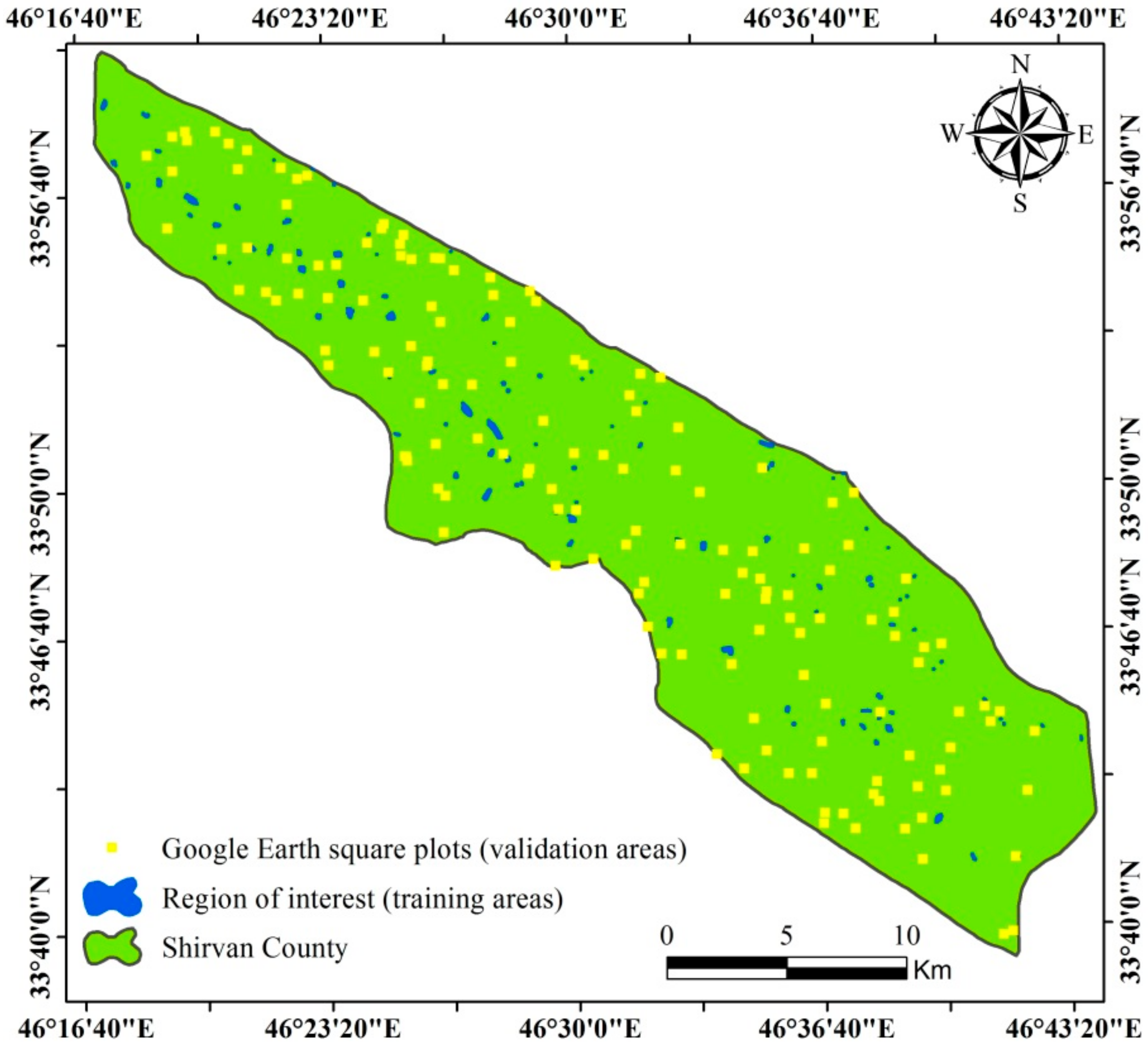
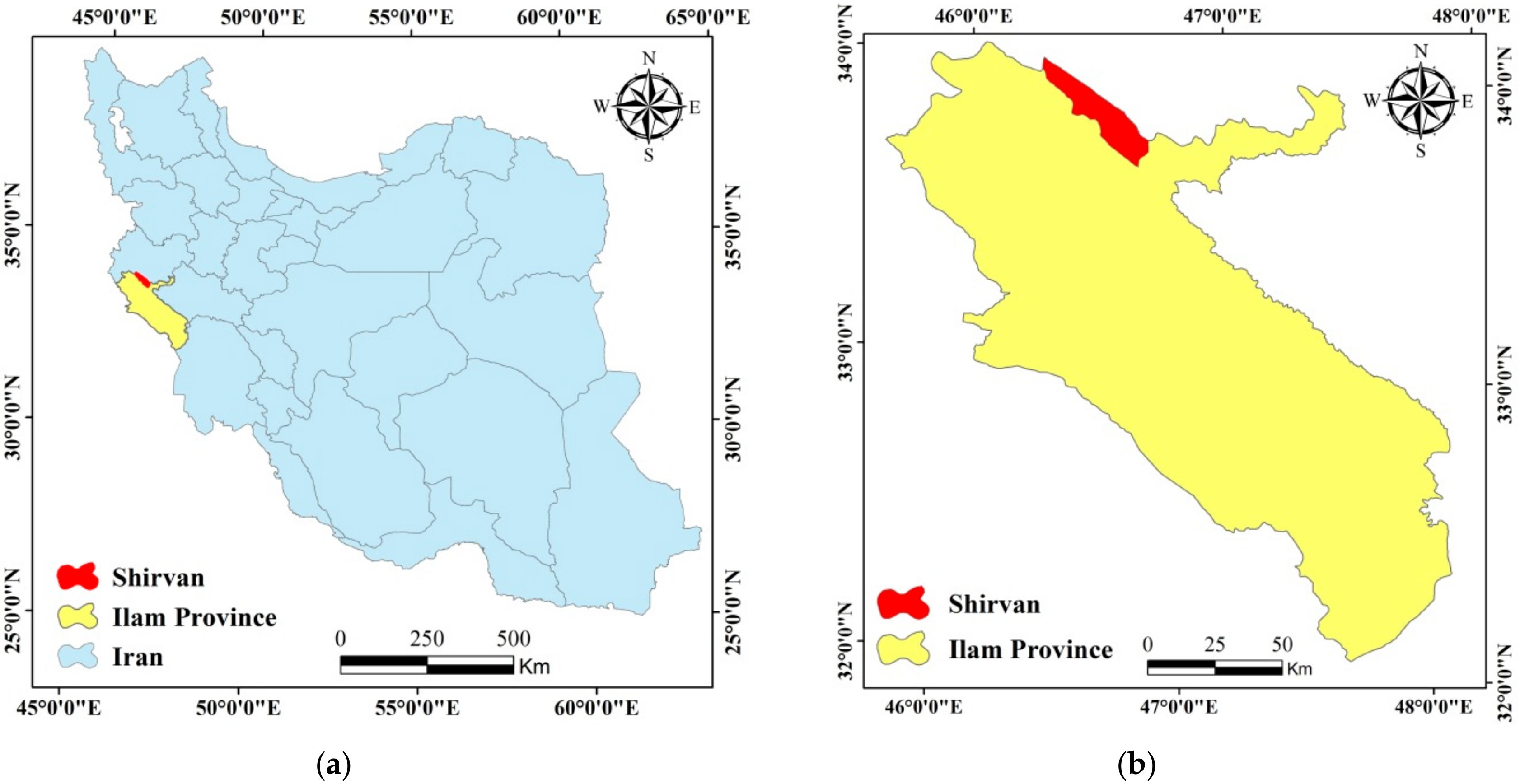
The study area is Shirvan County, situated in the northeast of Ilam Province in Iran, between 618,000 to 663,000 East longitude and 3,720,000 to 3,765,000 North latitude in WGS 1984_UTM Zone of 38 N (Figure 1). Shirvan County, with an area of about 45,355 ha, is located in a semi-arid region of Zagros Mountain. In this area, human interference (harvesting the wood and forest sub-products, converting the forests to the agricultural lands, grazing) and natural events (drought event, fire occurrence) have produced significant disturbances in the ecosystems. Additionally, agricultural lands have widely extended in this area in recent years. Still, the forest remnants are of high ecological value. Previous reports stated the Zagros forests in Western Iran are the oldest oak forests in the world with 5500 year old trees [5,6,7,8]. The main tree species in the study area are oak (Quercus brantii and Quercus persica), pistachio (Pistacia atlantica), almond (Amygdalus orientalis and Amygdalus scoparia), wild almond (Prunus scoparia), hackberry (Celtis caucasica), hawthorn (Cratagus aronia), and fig (Ficus johanis), which provide a unique habitat for many endemic animal species such as the Persian squirrel (Sciurus anomalus), Iranian leopard (Panthera pardus tulliana), Eurasian hog (Sus scrofa), wild goat (Capra aegagrus), Iranian gazelle (Gazella subgutturosa), ruppell’s fox (Vulpes rueppellii), etc. [2,65]. Some animal species like the Persian squirrels have an essential role in the regeneration, proliferation, and growth of some tree species such as oak trees [10,11,66].

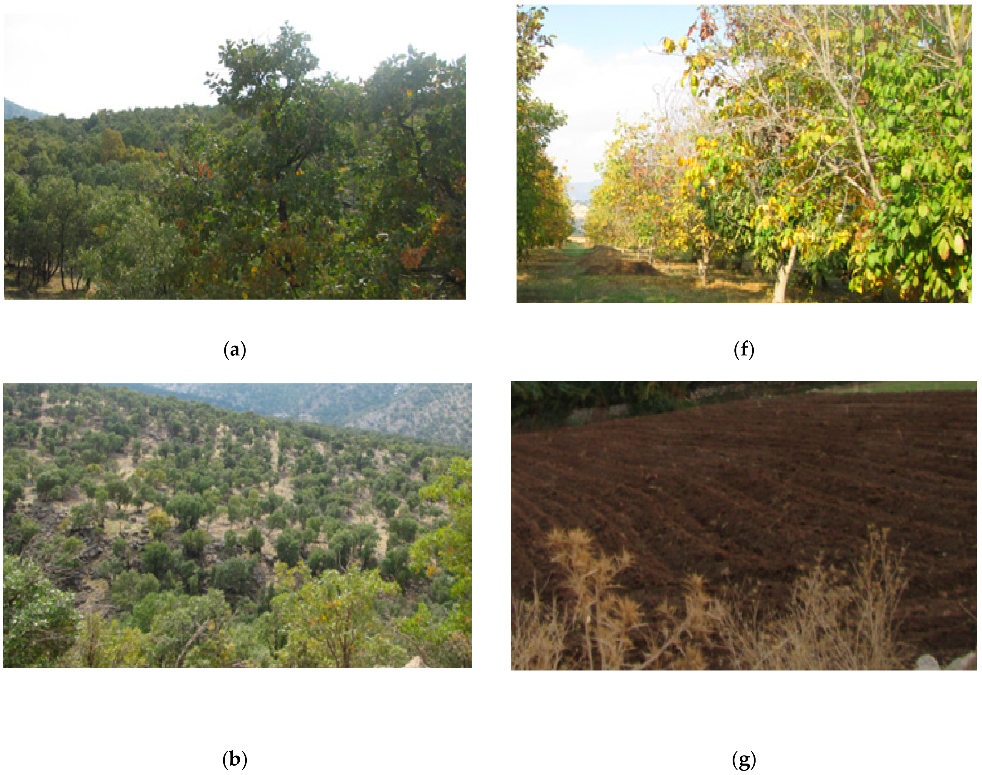
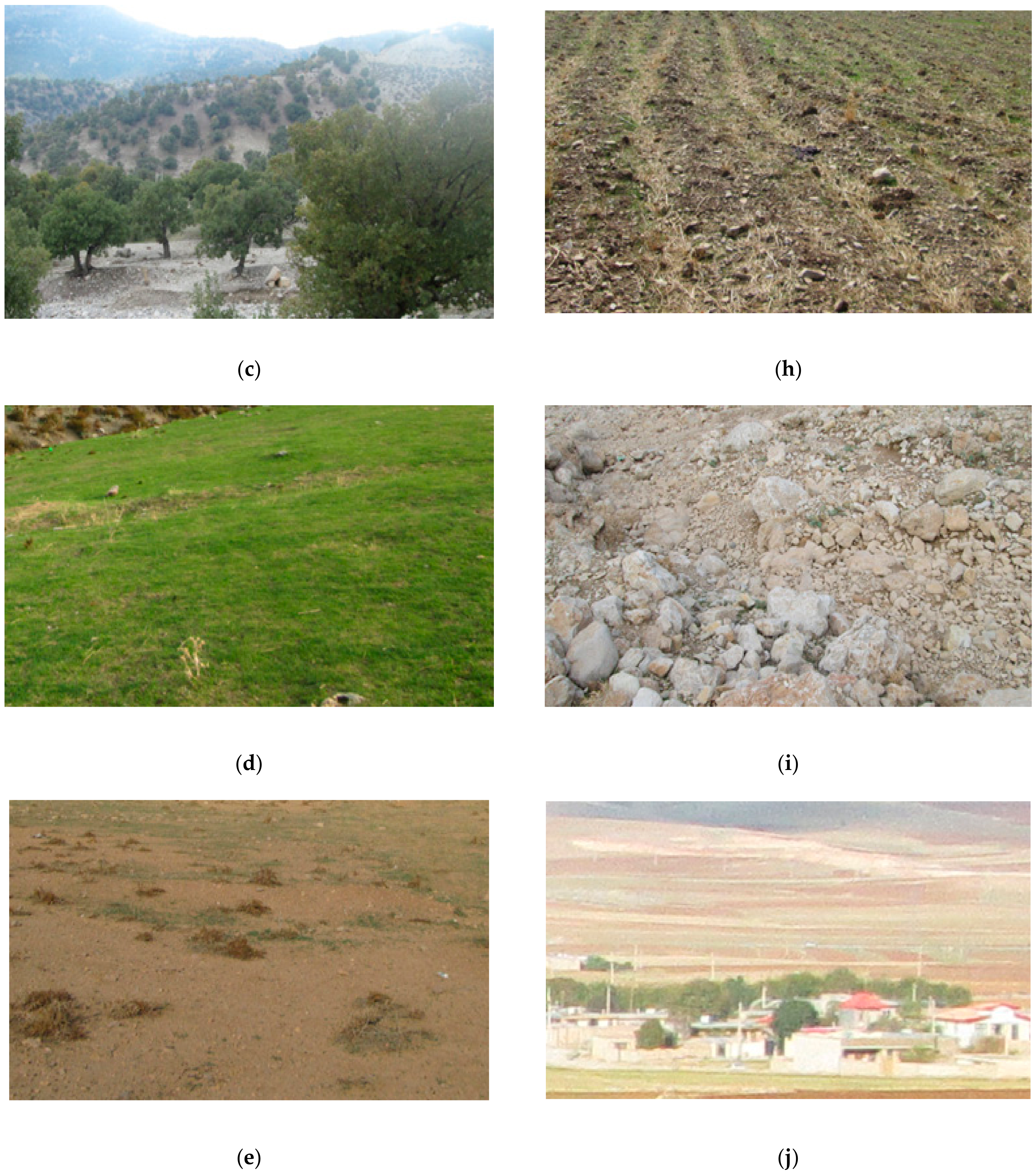
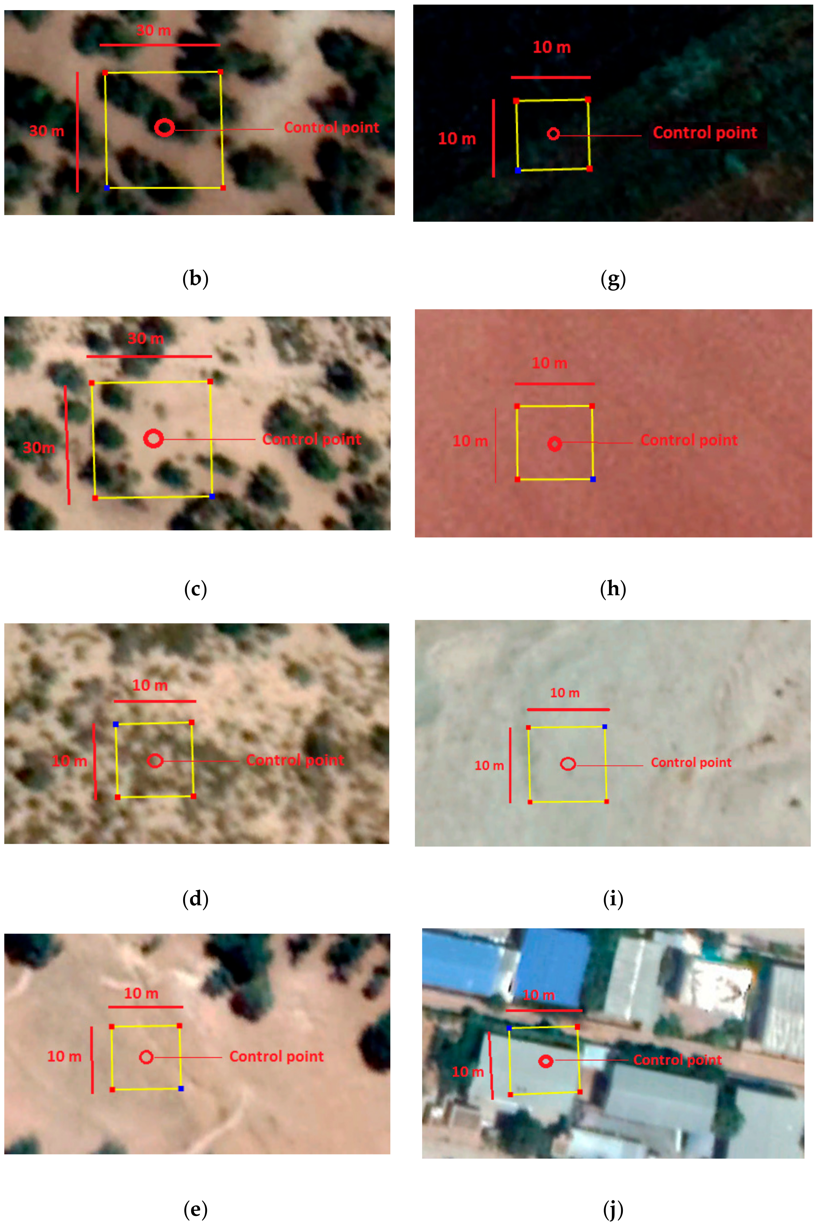
The land cover types considered in the study area are dense forest, semi-dense forest, sparse forest, dense rangeland, sparse rangeland, garden, irrigated farmland, dry farmland, bare soil, and urban area. The characteristics of these land cover classes are unique, and they proved to be spectrally different (Figure 2). Zagros forests are known as the oak forests of Iran as the dominant tree species is Quercus brantii and other tree species are very limited (Figure 3a–c) [8,9,12]. Therefore for land cover mapping in this study, we considered one tree species for forest cover (Quercus brantii), but different forest densities (three classes described in Section 2.3.1) (Figure 3a–c).

2.2. Data

For this research, we used two data sets for land cover and tree canopy cover mapping in Shirvan County: (1) Sentinel-2 images and (2) reference data including field data and Google Earth high-resolution data. The detailed descriptions of these data (date, resolution, and reference of data) are described below.

2.2.1. Sentinel-2 Images

Sentinel-2 is a wide-swath, high-resolution, multi-spectral imaging mission developed by ESA (European Space Agency) as part of the Copernicus Programme, supporting the Copernicus land monitoring services [67]. Sentinel-2 has 13 spectral bands with a spatial resolution from 10 to 60 m (

Table 1. The spectral bands of Sentinel-2 data.

Band Number	Band Name	Wavelength Mean (nm)	Spatial Resolution (m)
B01	Coastal aerosol	443	60
B02	Blue	490	10
B03	Green	560	10
B04	Red	665	10
B05	Vegetation Red Edge	705	20
B06	Vegetation Red Edge	740	20
B07	Vegetation Red Edge	783	20
B08	NIR	842	10
B08a	Narrow NIR	865	20
B09	Water Vapor	945	60
B10	SWIR-Cirrus	1375	60
B11	SWIR	1610	20
B12	SWIR	2190	20

).

For this research, we used the Sentinel-2 Level-1C product. The Level-1C product is composed of 100 × 100 km² tiles (Ortho-images in UTM/WGS84 projection). This product results from using a digital elevation model (DEM) to project the image in cartographic geometry. Level-1C products are resampled with a constant ground sampling distance (GSD) of 10, 20, and 60 m depending on the native resolution of the different spectral bands [67]. We selected Sentinel-2 data in this study because of its better spatial resolution (10 m) rather than Landsat-8 (30 m). In recent years, the application of the Sentinel-2 satellite image for land use/land cover mapping has been very successful in different areas around the world [30,31,32,33].

For this research, we obtained the Sentinel-2 Level-1C satellite image for the study area (28 July 2017) from the ESA website (https://scihub.copernicus.eu) (Figure 4).

FRWOI provided the vector map of Shirvan County in Ilam Province. Then, the Sentinel-2 satellite data was clipped to focus the classification on Shirvan County, which was our study area (Figure 4).

2.2.2. Reference Data

In this study, we used field data and Google Earth’s high-resolution data as reference data. Field data of 300 square plots (see Section 2.3.1) were used for the TCC% estimation and also the accuracy assessment of the Google Earth data. Later, we used Google Earth data for the accuracy assessment of the land cover maps obtained from Sentinel-2 (see Section 2.3.3). We selected images from 2017 to 2019 with 65 × 65 cm spatial resolution. The advantages of using Google Earth data are that they are high-resolution (65 × 65 cm), are available for free, and depict the imagery date [68,69]. Google Earth’s high-resolution data have been widely used as reference data in many studies. Previous research proved the horizontal and vertical precision of these images [68,69,70,71,72]. Although the overall accuracy of Google Earth data is established in the literature, we considered it appropriate to assess the accuracy of the images in our study area. For this research, we used Google Earth data acquired in 2017.

2.3. Research Method

2.3.1. Accuracy Assessment of Google Earth Data Using Field Data

We assessed the accuracy of Google Earth data using several control points and square plots in the field. Figure 3 shows the different land covers in the field in the study area, Shirvan County. For this purpose, we randomly collected 300 control points in the center of 300 square plots during a field visit in July 2019 (Figure 4). Due to the heterogeneous landscape of the study area, we used a random sampling strategy in this study [39,45,46,49,50]. The 300 field square plots included 30 plots for each land cover type (there were 10 land cover types, including both forest cover classes and non-forest cover classes). The center of 300 square plots was found by GPS (global positioning system) (Model: Garmin Map 64S C) that had an accuracy of less than 1 m.

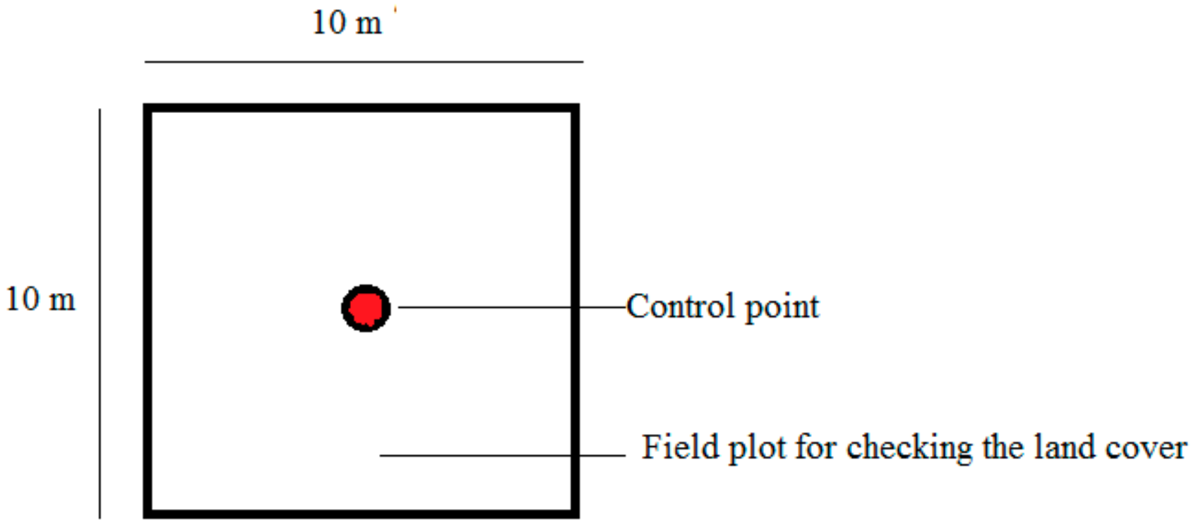
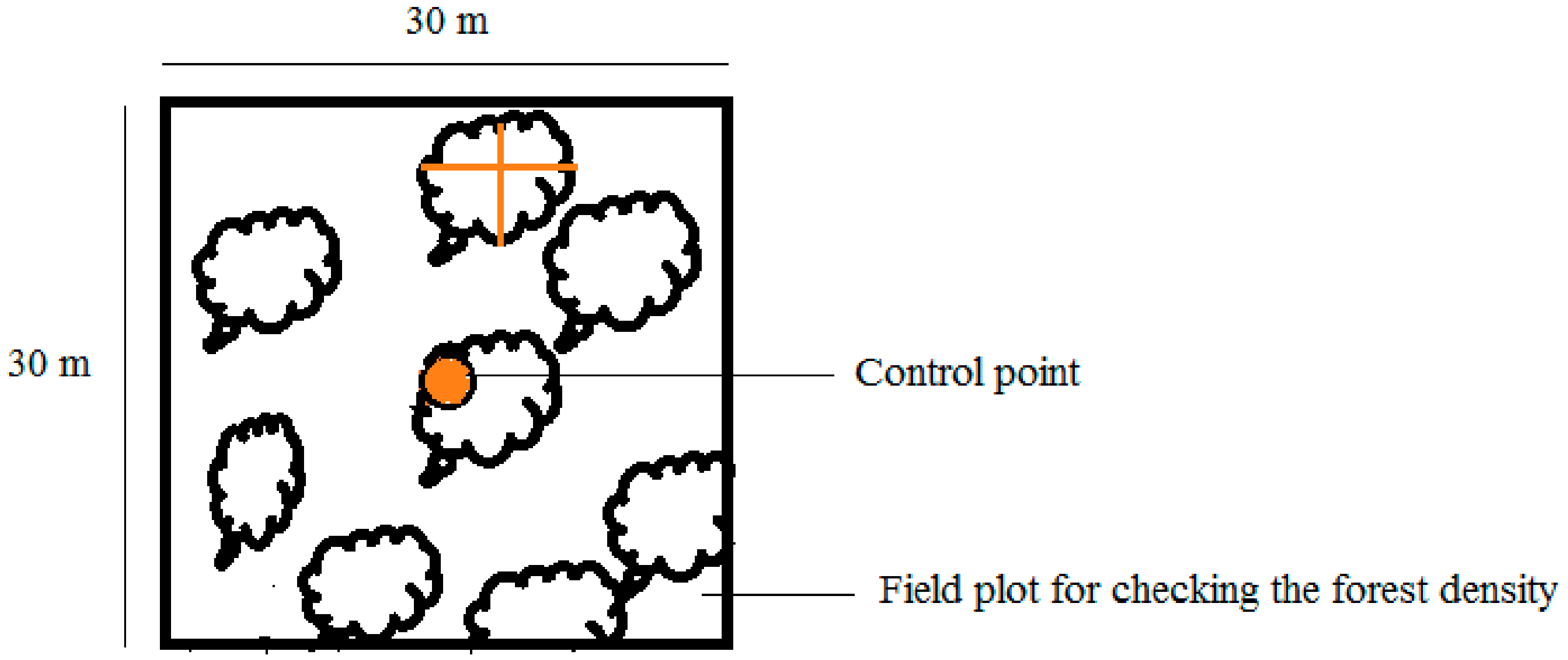
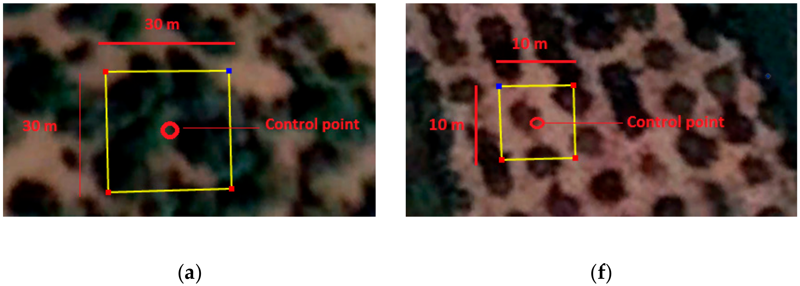
For each non-forest land cover (dense rangeland, sparse rangeland, garden, irrigated farmland, dry farmland, bare soil, and urban area), thirty 10 × 10 m square field plots were taken, which corresponded to the pixel size of the Sentinel-2 images (Figure 5). In the case of forest cover (dense forest: >50% tree canopy cover, semi-dense forest: 25–50% tree canopy cover, sparse forest: 5–25% tree canopy cover), we took 30 30 × 30 m square field plots, corresponding to 3 × 3 pixels of the Sentinel-2 images (Figure 6). The dimension of 30 × 30 m for square forest plots was selected because of the diameter of the tree crown (5–8 m) in the study area [65] and based on recommendations of previous studies [22]. We noted that the estimation of tree canopy cover in a 10 × 10 m square plot might be possible. Still, it probably creates some errors in tree canopy cover estimation, because based on FRA definition, the forest is a land with at least 0.5 ha area with trees higher than 5 m [73]. Therefore, we considered an area of 900 m²⁻ (3 × 3 pixels of the Sentinel-2 images) to establish square field plots in forest cover. Consequently, we applied 30 × 30 m square plots in forest covers and 10 × 10 m square plots in other land covers.

There was a temporal difference of two years between the field data (summer 2019) and the Sentinel-2 data (summer 2017) because the image processing of the Sentinel-2 image was performed before fieldwork. We needed to obtain a general map of land cover in the study area to allocate the square plots in different land covers in the field. After that, we designed our fieldwork to sample 300 square plots. Therefore, the date of the Sentinel-2 image was before the date of field sampling. However, the season of Sentinel-2 image and field surveys were the same (summer) to prevent some errors because of physiologic and phenologic differences in the field and satellite image. In addition, the cutting of trees was prohibited in the study area during the time between 2017 and 2019, and potential changes in tree cover were assumed to be minor [22].

Our purpose was the measurement of dry-season NDVI (summer) in this study [22]. This was because the results of previous studies have shown that the dry-season NDVI was positively related to tree canopy cover changes, both across space and time [22,45].

2.3.2. Land Cover Mapping Using Supervised Classification Algorithms

For land cover mapping, we used a combination of bands B02, B03, B04, and B08 of the Sentinel-2 satellite image because of their enhanced spatial resolution (10 m). In this study, we preferred spatial resolution to spectral resolution of the bands to determine different land covers. This was because the selection of four bands in visible and near-infrared spectral range was good enough to separate the predictable land covers in our study area (forest, rangeland, garden, irrigated farmland, dry farmland, bare soil, and urban area) (Figure 2). However, the separation of different forest density classes was more challenging. For this purpose, we applied a proper vegetation index (dry-season NDVI) which is described in Section 2.3.4.

After layer stacking of bands B02, B03, B04, and B08, we applied four supervised classification algorithms to produce an accurate 10 m resolution land cover map: minimum distance (MD), Mahalanobis distance (MaD), neural network (NN), and support vector machine (SVM). These algorithms were selected due to their ability to adapt to the heterogeneous structure of the study area, the spatial resolution of a satellite image (10 m), and their suitability for land cover classification in the previous studies [17,30,33,36,41,74,75].

For the algorithm application, we selected a set of training pixels from the Sentinel-2A image for each land cover type. Based on the predictable land covers (dense forest, semi-dense forest, sparse forest, dense rangeland, sparse rangeland, garden, irrigated farmland, dry farmland, bare soil, and urban area) in the study area, regions of interest (ROI) were selected as pixel-based samples. We considered a minimum number of 500 pixels as a training area for each land cover class. Then, we applied the supervised classification algorithms on the Sentinel-2 image for land cover mapping of the study area. The applied algorithms are described below.

Minimum Distance (MD)

In the minimum distance algorithm, all pixels are classified to the nearest class unless a standard deviation or distance threshold is specified, in which case some pixels may be unclassified if they do not meet the selection criteria. The minimum distance classifier computes the Euclidean distance (ED) between the pixel values (xp,yp) and the mean values for the classes. It then allocates the pixel to the class with the shortest Euclidean distance [76,77].

Mahalanobis Distance (MaD)

The Mahalanobis distance classification is a direction-sensitive distance classifier that uses statistics for each class. It is similar to the maximum likelihood classification but assumes that all class co-variances are equal, and therefore, it is a faster method. The advantage of the Mahalanobis classifier over the maximum likelihood procedure is that it is faster and yet retains a degree of direction sensitivity via the covariance matrix C, which could be a class average or a pooled covariance [78]. All pixels are classified to the closest region of interest (ROI) class unless a distance threshold is specified, in which case some pixels may be unclassified if they do not meet the criteria [79].

Neural Network (NN)

The most popular neural network classifier in remote sensing is the multilayer perceptron. Feedforward or multilayer perceptrons (MLP) may have one or more hidden layers of neurons between the input and output layers [80]. They have a simple layer structure in which successive layers of the neuron are fully interconnected, with connection weights controlling the strength of the connections. The input to each neuron in the next layer is the sum of all its incoming connection weights multiplied by their connecting input neural activation value [80,81]. This method is independent of the statistical parameters of a particular class and accepts qualitative and quantitative data to be introduced as input data.

Support Vector Machine (SVM)

The SVM algorithms are non-linear binary classifiers and aim to find a threshold that divides the dataset into the predefined classes using training samples [82]. The optimal separation is applied to minimize misclassifications, which usually occur in the training step [41,83]. Considering the principles of structural risk minimization [84,85], SVMs aim to minimize the upper bound of the expected generalization error by maximizing the margin between the separating hyperplane and the data. The concept of margin plays a key role in the SVM algorithm as it indicates the generalization capability of SVMs [86,87]. The main advantage of SVMs is the ability to transform the model to solve a non-linear classification problem without any prior knowledge [33].

2.3.3. Accuracy Assessment of Land Cover Maps Using Google Earth Data

Many researchers have expressed opinions about the proper sampling scheme to use for accuracy assessment. Five common sampling schemes were applied for collecting reference data/accuracy assessment: (1) simple random sampling, (2) systematic sampling, (3) stratified random sampling, (4) cluster sampling, and (5) stratified, systematic, unaligned sampling [88].

To perform the accuracy assessment of the land cover classifications in this research, we generated a stratified random sampling of 150 points (Figure 7). We randomly distributed a number of points in each class proportional to the area of each class [89]. We selected the stratified sampling method [88] because this method proved to be more appropriate than a systematic-random method for the determination of forest areas in the Zagros Mountains, as reported in previous studies [90]. Additionally, stratified random sampling has been highly recommended in previous studies concerning assigning sufficient samples to each land cover type for the accuracy assessment of the classified maps [21,22]. Finally, coordinates of stratified random points were extracted, and the locations were visited in Google Earth Pro 7 to record their land cover class.

We obtained Google Earth data in July 2017, coinciding with the date of Sentinel-2 imagery. In Google Earth, we checked the actual cover of each control point of non-forest classes in a square plot of 10 × 10 m, which was concordant to the pixel dimension in the Sentinel-2 image (Figure 5). The land cover of each control point in the forest density classes was checked in a square plot of 30 × 30 m, which was accordant to the 3 × 3 pixel size in the Sentinel-2 image and also to the dimension of the forest field plots (Figure 6). Figure 8 shows the method for checking the different land cover types in plot areas in Google Earth Pro.7.

Then, we compared the Google Earth land cover classes and the classified land cover classes in the 150 random points to assess the accuracy of the classification algorithms. The calculated accuracy metrics in this study were the overall accuracy (OA) and the kappa index ($\widehat{k}$) [88,91].

2.3.4. Forest Density or TCC% Estimation Based on Fieldwork and the NDVI

Forest density mapping is an essential subject for forest management because proper management and planning are required for each category of forest density. For example, in the western forests of Iran (Zagros forests), the dense forests’ biodiversity should be protected, because this forest category provides a valuable habitat for much unique fauna and flora in Western Iran. On the other hand, the semi-dense forest requires planning for soil and water conservation in the Zagros Mountains as the erosion risk is an essential factor [9,12,17]. The sparse forests are the most fragile ecosystems in Western Iran. If they are not protected, they are at risk of being converted to farmland and urban area in the future [17].

The forest density is defined by the TCC in Iran [92]. The TCC is the land area that is covered by tree canopy when viewed from above [22].

First, the forest cover (including three density classes described in Section 2.3.1) was classified on the Sentinel-2 imagery. Then, we used the field data of three forest density classes (including tree canopy cover in each forest plot) to separate the forest density classes. Three forest densities were considered, which we estimated in 90 square plots with dimensions of 30 × 30 m (30 square plots for each forest density class) in the field (Figure 6). In each forest density class, we measured in the field two diameters of the crowns of all trees inside the square plots (Figure 6). The diameters were taken in north-south and east-west directions (Figure 6) for all trees inside a certain plot (Figure 6). We did not measure diameters of the tree crowns on Google Earth, but we measured all of them in the field by meter tape.

Based on our measurements in the field, we did not find a big difference between the two diameters (north-south and east-west) of the crown of most trees. Therefore, we assumed that the tree crowns followed a circle shape (for instance, two diameters of the crown of a tree inside a plot were 5.5 and 6 m). Therefore, we calculated the average of two diameters of each tree in each square plot. It was divided by two to obtain the radius (r) of the crown of each tree. By assuming that a tree crown is a circle, the canopy area of each tree was calculated based on the circle area formula (πr²). Then, assuming the same area for every tree in the plot we calculated the sum of the canopy areas of all trees in each square plot. Finally, the canopy cover for each forest square plot was calculated based on the relationship of the sum of tree canopy areas to the square plot area (900 m²). Thus, the canopy cover percentage for each forest square plot was calculated as below:

$$\mathrm{Canopy} \mathrm{Cover} \mathrm{Percent}=\frac{\sum \begin{array}{c}\mathrm{n}\\ \mathrm{i}=1\end{array}\mathrm{TCCA}}{\mathrm{SPA}}\times 100$$

(1)

where TCCA is a tree canopy cover area, and SPA is a square plot area that is 900 m² (30 × 30 m = 900) in this study.

For some plots in the dense forest, there was a little overlapping among some tree crowns inside a plot. However, we measured the diameters of all trees inside the plot. Our final purpose was an estimation of tree canopy cover (relation of the sum of canopy areas of all trees to the square plot area). Therefore, this overlapping cannot create many errors in such estimation. Based on its definition, the tree canopy cover (TCC) is the land area that is covered by tree canopy when viewed from above [22]. If the overlapping is high, the TCC% may obtain more than 100%. However, we did not have TCC% more than 100% in our records, as the highest TCC% obtained in our measurements was 95%.

As mentioned before (Section 2.3.2), we used a combination of bands B02, B03, B04, and B08 for land cover mapping such as primary forest cover mapping, because of their enhanced spatial resolution (10 m). Then, for canopy cover estimation in forest cover, we used the NDVI as a standard vegetation index and predictor variable in the estimation of the TCC%, which resulted in a nicely fitted correlation with forest canopy cover in previous studies [22,23,42,43,44,45,46,48,50,51]. In fact, for more exact analysis, we used dry-season NDVI for separating different forest density classes. Among all vegetation indexes, we used the NDVI in this study because this index has yielded a better correlation with tree canopy cover than other vegetation indices, especially in the dry season [22,45]. It has been the most reliable vegetation index in forest density estimations [22,42,43,44,46,51]. The NDVI is described below [23,93]:

$$\mathrm{NDVI}=\frac{NIR-RED}{NIR+RED}$$

(2)

where NIR is the spectral reflectance in the near-infrared wavelength (0.85–0.88 μm) and RED is the spectral reflectance in the red wavelength (0.64–0.67 μm) [23,93].

We then calculated the NDVI for the forest cover of Shirvan County and extracted the NDVI values for each forested square plot. Then, the correlation between the tree canopy cover percentage (TCC%) (obtained from field plots) and the NDVI value was calculated by using the Pearson correlation coefficient. We produced a fitted linear regression model between the TCC% and the NDVI values. Based on these analyses, a predictive model of the TCC% based on the NDVI was developed. We applied the model to all the forest cover types in Shirvan County to estimate the canopy cover percentage map for the whole forest area. Finally, this map was classified into three classes of forest density (sparse: 5–25%, semi-dense: 25–50%, and dense: >50% canopy cover percentage).

3. Results

3.1. Accuracy Assessment of the Google Earth Data Using Field Plots

The results of the accuracy assessment of the Google Earth data using 300 square field plots are shown in

Table 2. The confusion matrix of comparison of the control plots in the Google Earth (predicted) and in the field (observed).

		Number of Control Plots in Google Earth (Predicted)
	Land Cover	Dense Forest	Semi-Dense Forest	Sparse Forest	Dense Rangeland	Sparse Rangeland	Garden	Irrigated Farmland	Dry Farmland	Bare Soil	Urban Area	Total
Number of Control Plots in the Field (Observed)	Dense forest	29	0	0	0	0	0	0	0	0	0	29
	Semi-dense forest	1	27	0	0	0	0	0	0	0	0	28
	Sparse forest	0	0	25	0	0	0	0	2	0	0	27
	Dense rangeland	0	0	0	28	0	0	1	0	0	0	29
	Sparse rangeland	0	0	0	0	28	0	0	0	0	0	28
	Garden	0	0	0	0	2	30	0	0	0	0	32
	Irrigated farmland	0	0	0	2	0	0	29	0	0	0	31
	Dry Farmland	0	0	5	0	0	0	0	28	0	0	33
	Bare soil	0	3	0	0	0	0	0	0	30	0	33
	Urban area	0	0	0	0	0	0	0	0	0	30	30
	Total	30	30	30	30	30	30	30	30	30	30	300

and

Table 3. Evaluating the accuracy of Google Earth data using 300 field plots.

Land Cover in Google Earth	Land Cover in the Field	Number of Square Plots	Number of True Classified Square Plots	Overall Accuracy (%)
Dense forest	Dense forest	30	29	96
Semi-dense forest	Semi-dense forest	30	27	90
Sparse forest	Sparse forest	30	25	83
Dense rangeland	Dense rangeland	30	28	93
Sparse rangeland	Sparse rangeland	30	28	93
Garden	Garden	30	30	100
Irrigated farmland	Irrigated farmland	30	29	96
Dry Farmland	Dry Farmland	30	28	93
Bare soil	Bare soil	30	30	100
Urban area	Urban area	30	30	100
Total	Total	300	284	94.4

. Table 2 shows the confusion matrix comparing the control points in the Google Earth (predicted) and in the field (observed). The overall accuracy of the 10 land cover types was completely different. Based on the results in Table 2, garden, bare soil, and urban area, with an overall accuracy of 100%, yielded the highest accuracy based on field data. The dense rangeland and sparse rangeland have shown the same accuracies (overall accuracy of 83%). The irrigated farmland obtained a slightly higher accuracy than dry farmland in Google Earth. About forest density classes, the accuracy of Google Earth decreased from the dense forest to the sparse forest, so that sparse forest, with an overall accuracy of 83%, resulted in the lowest accuracy of all land cover types (Table 3). The results of Table 3 show that the Google Earth data, with an overall accuracy of 94.4%, has shown a reliable accuracy as reference data in this study.

3.2. Land Cover Maps

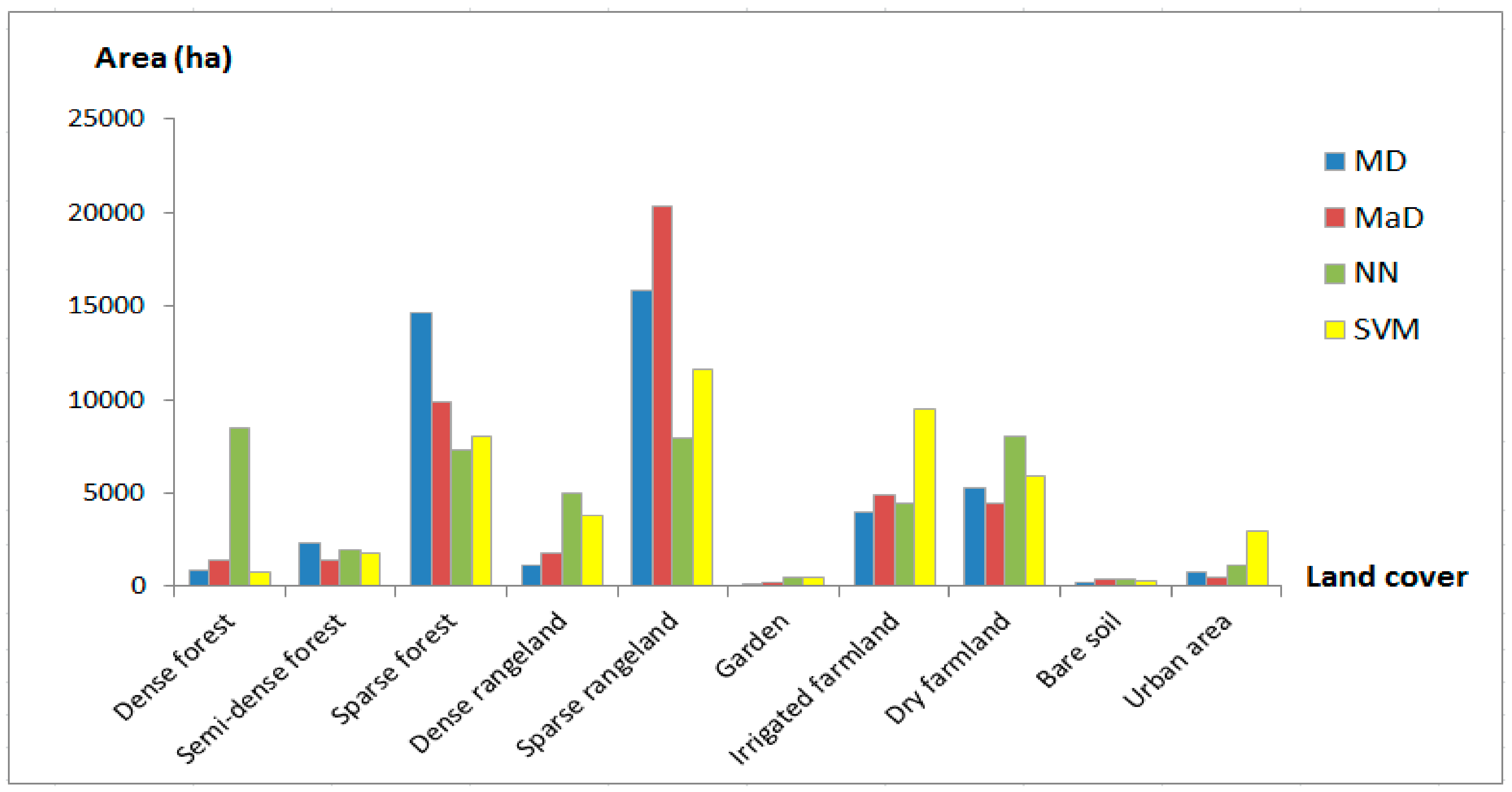
We produced four land cover maps of Shirvan County by classifying a Sentinel-2 image using different supervised algorithms: minimum distance, Mahalanobis distance, neural network, and support vector machine (Figure 9). Areas of land cover classes based obtained from the different algorithms are reported in Figure 10.

All the land cover maps showed a similar spatial distribution of the land cover classes as the other three methods (MD, MaD, SVM). However, we noted that the NN land cover map (Figure 9c) classified a large area as dense forest 8–10 times larger than the area classified as dense forest by the other methods (Figure 10). Based on some observed reports, the dense forest area is limited to a specific region in the study area, because many oak trees were affected by drought events in the Ilam Province in recent years [65]. The official report states that there are only 2594 ha of dense forests in the Ilam Province [65]. Analyzing the results, we concluded that the NN algorithm classified areas of semi-dense forest as dense forest, thus producing the overestimation of the latter.

Between the MD (Figure 9a), MaD (Figure 9b), and SVM (Figure 9d) algorithms, we observed the most substantial differences in the classes of the sparse forest, sparse rangeland, and irrigated farmland. The MD classified a larger area as sparse forest compared to the other two methods, whereas the MaD mapped a broader area as sparse rangeland. The SVM yielded an area of irrigated farmland that was twice the size of that produced by the MaD and MD classifiers. In general, the SVM land cover map (Figure 9d) classified an area of the dense forest of 777.13 ha, which is coincident with our field observations. In addition, the location of sparse forests in the northeast of Shirvan County is correct. Additionally, the SVM classified dense and semi-dense forests in the southwest of the study area, exactly where they were found in the field. Farmlands extend over a wide area of Shirvan County, whereas urban areas locate in the middle of Shirvan County and are surrounded by sparse rangelands. This qualitative evaluation of the method suggests that the SVM classifier is more accurate than the other classifier methods used in this study.

3.3. Accuracy Assessment of Land Cover Maps Using Google Earth Data

We performed the accuracy assessment of all the algorithms by computing the overall accuracy and kappa index (

Table 4. The accuracy assessment of supervised classification algorithms.

Classification Algorithm	Overall Accuracy (%)	Kappa Index
Minimum distance (MD)	68	0.57
Mahalanobis distance (MaD)	72.67	0.63
Neural network (NN)	48.67	0.38
Support vector machine (SVM)	81.33	0.76

). The SVM algorithm has the highest accuracy in land cover mapping with an overall accuracy of 81.33% and a kappa index of 0.76 (Table 4). These results show that the land cover map obtained from SVM is more accurate than other land cover maps. Therefore, the areas of different land covers based on this algorithm represent the reality better than other algorithms. After the SVM method, the MaD stands out with an overall accuracy of 72.67% and a kappa index of 0.63. In contrast, the NN algorithm with an overall accuracy of under 50% and kappa index values of less than 0.5 presents the lowest accuracy of the land cover mapping of Shirvan County (Table 4).

For further analysis of the accuracy assessment of the SVM land cover map, the confusion matrix comparing the control plots in the land cover map (classified land cover) and Google Earth (reference data) is shown in

Table 5. The confusion matrix of comparison of control plots in support vector machine (SVM)-land cover map (classified) and Google Earth (reference).

		Number of Control Plots in Land Covers in SVM Map (Classified Map)
	Land Cover	Dense Forest	Semi-Dense Forest	Sparse Forest	Dense Rangeland	Sparse Rangeland	Garden	Irrigated Farmland	Dry Farmland	Bare Soil	Urban Area	Total
Number of Control Plots in Land Covers in Google Earth (Reference)	Dense forest	6	0	0	0	0	0	0	0	0	0	6
	Semi-dense forest	0	8	0	0	0	0	0	0	4	0	12
	Sparse forest	0	0	20	0	0	0	0	6	0	0	26
	Dense rangeland	0	0	0	12	0	0	4	0	0	0	16
	Sparse rangeland	0	0	0	0	22	1	0	0	0	0	23
	Garden	0	0	0	0	1	7	0	0	0	0	8
	Irrigated farmland	0	0	0	7	0	0	19	0	0	0	26
	Dry Farmland	0	0	2	0	0	0	0	12	0	0	14
	Bare soil	0	3	0	0	0	0	0	0	7	0	10
	Urban area	0	0	0	0	0	0	0	0	0	9	9
	Total	6	11	22	19	23	8	23	18	11	9	150

. In

Table 6. Accuracy assessment of land covers obtained from the SVM algorithm by Google Earth data.

Land Cover	Number of Control Plots (Reference) in Google Earth	Number of True Classified Control Plots in SVM-Land Cover Map	Overall Accuracy (OA)
Dense forest	6	6	100%
Semi-dense forest	12	8	66%
Sparse forest	26	20	77%
Dense rangeland	16	12	75%
Sparse rangeland	23	22	96%
Garden	8	7	87%
Irrigated farmland	26	19	73%
Dry farmland	14	12	86%
Bare soil	10	7	70%
Urban area	9	9	100%
Total	150	122	81.3%

, we represent a more detailed analysis of the accuracy of the most accurate map (SVM) by land cover class.

3.4. Forest Density or TCC% Mapping

3.4.1. NDVI Map of Forest Cover

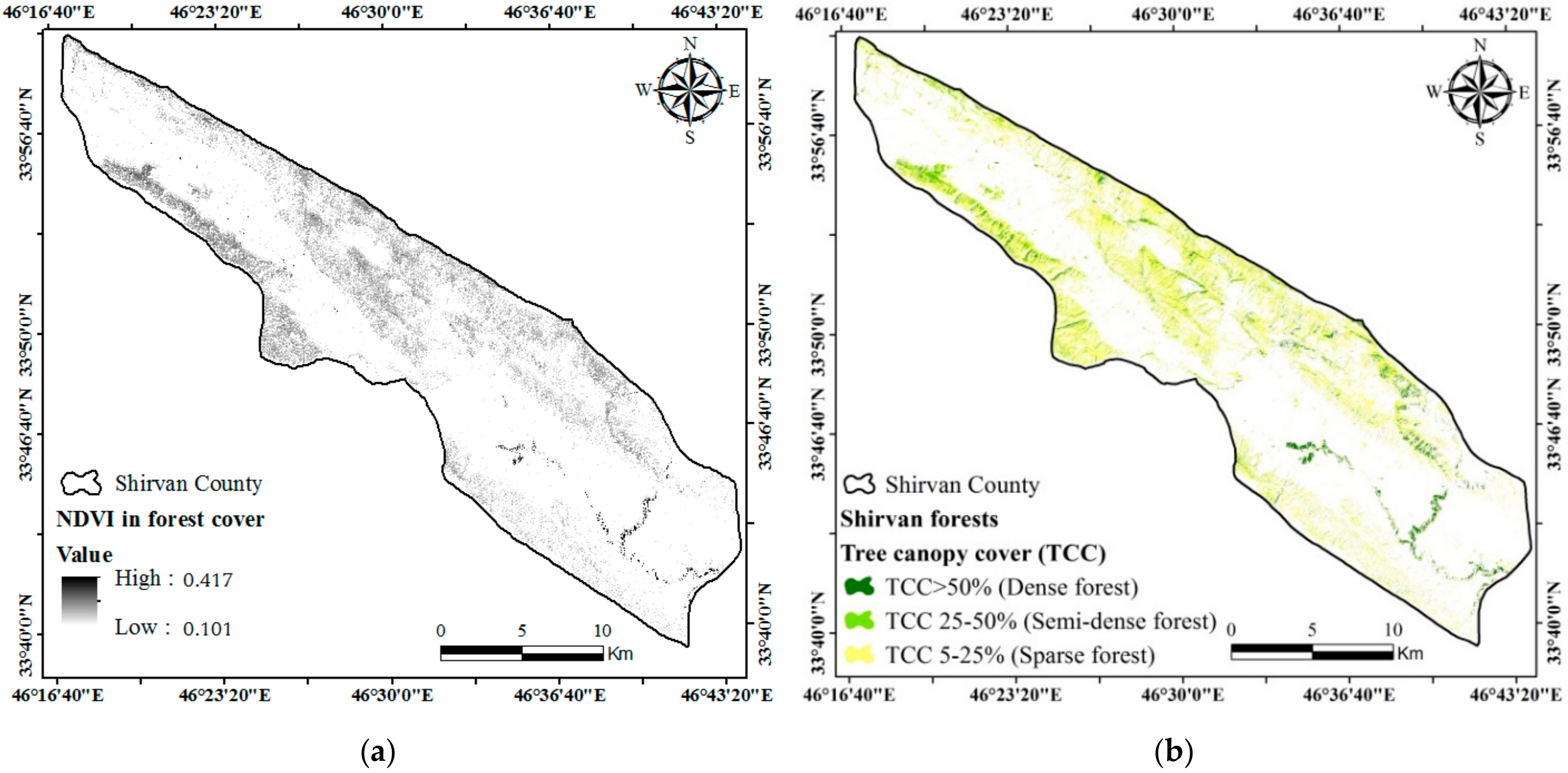
The results show that the NDVI forest cover values range from 0.101 to 0.417 in Shirvan County (

Table 7. Details of normalized difference vegetation index (NDVI) and tree canopy cover (TCC)% obtained from field plots for each forest density class.

Forest Density Class	Standard Canopy Cover (%)	Number of Field Plots	TCC Percentage (%)				NDVI
			Min	Max	Mean	SD	Min	Max	Mean	SD
Sparse forest	5–25	30	5	25	16.36	7.25	0.101	0.206	0.181	0.028
Semi-dense forest	25–50	30	30	50	42.17	6.56	0.219	0.269	0.245	0.012
Dense forest	>50	30	55	95	73.88	10.99	0.272	0.417	0.334	0.037

). These results demonstrate that the NDVI values in the study area are not very high in comparison with other forests around the world [23,45]. It may be related to the health conditions of the Zagros forests in Shirvan County because these forests have gone through several drought events in recent decades.

3.4.2. Correlation between the TCC% and the NDVI and Predictive Regression Model for the TCC%

Results of the field plot data and the NDVI values for each TCC% class are shown in Table 7. Based on these results, the NDVI ranges from 0.101 to 0.206 in the sparse forest density class in the 30 plots. The canopy cover percentage ranges from 5% to 25% in the sparse forest, which is within the standard canopy cover percentages based on the FRWOI [92] classification.

For the semi-dense forest, the minimum NDVI is 0.219, and the maximum NDVI is 0.269, and the canopy cover percentage ranges from 30% to 50%.

In the dense forest, the NDVI has the highest value, with a maximum NDVI of 0.417 and a minimum NDVI of 0.272. The canopy cover ranges from 55% to 95%, which is within the range of the standard canopy cover percentage [92].

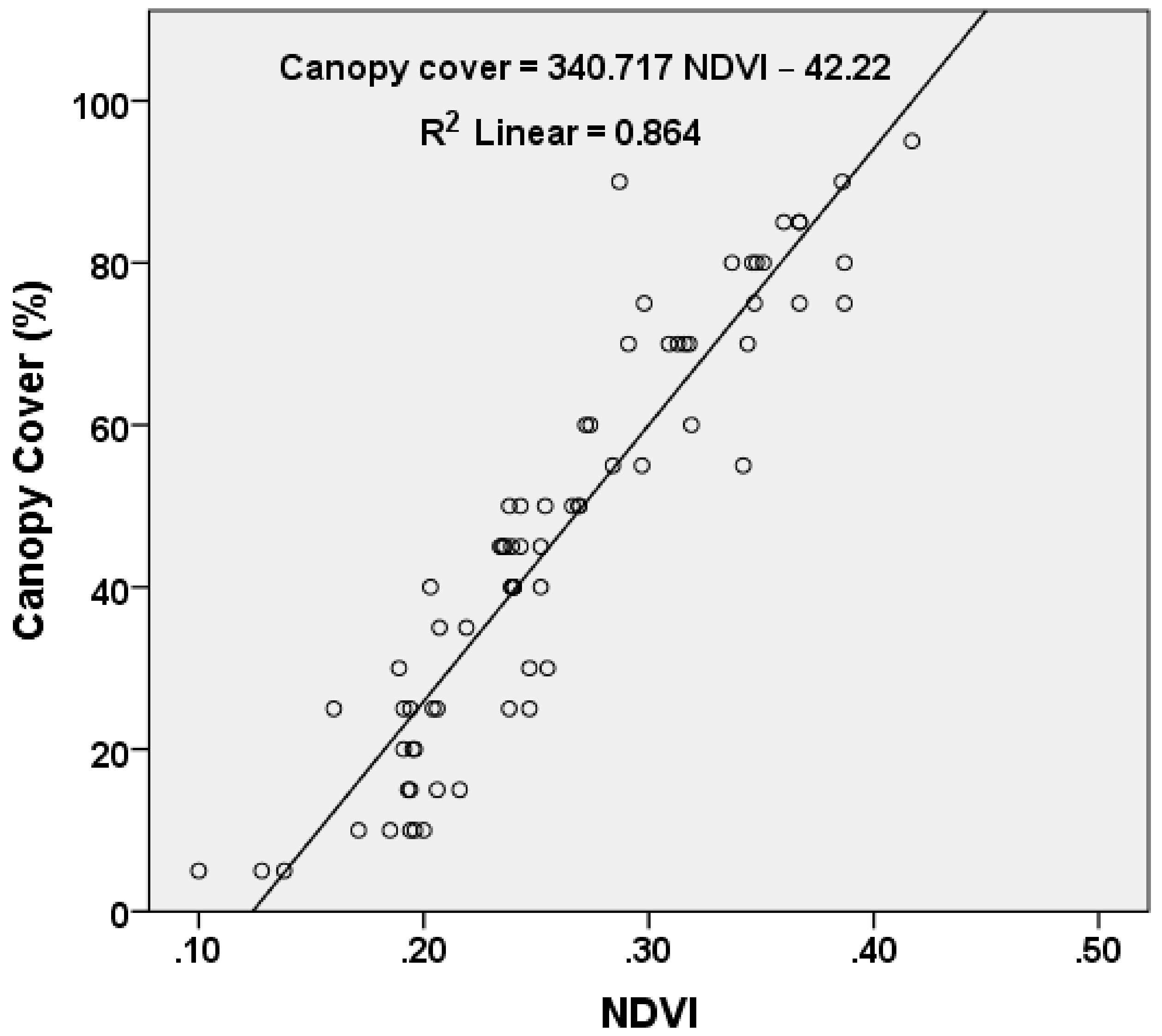
Results of the correlation coefficient between the TCC% and the NDVI showed that the Pearson correlation between these variables is 0.93, which is significant at the 99% confidence level (

Table 8. Correlation between the canopy cover percentage and NDVI.

Variable	n	Pearson Correlation	Sig.
NDVI	90	0.93 **	0.000
TCC%	90	0.93 **	0.000

** Significant at a 99% confidence level.

). The graphic plot shows that there is a linear correlation between the canopy cover percentage and NDVI values (Figure 11). Therefore, we applied linear regression method instead of random forest (RF) and SVM methods for predicting TCC% in this study. So far, many researchers have used this method to discover the relationship between the canopy cover and NDVI values in different forest areas around the world [21,23,45,50,51].

We performed a linear regression based on 90 sample plots in three forest density classes (dense forest, semi-dense forest, and sparse forest,

Table 9. Model summary of the TCC% based on the NDVI.

Model	R	R Square	Adjusted R Square	Standard Error of the Estimate
1	0.930 a	0.864	0.864	9.4607

a. Predicators: Constant, NDVI.

and

Table 10. Coefficients of the linear regression model between the TCC% and NDVI.

Model	Unstandardized Coefficients		Standardized Coefficients	t	Sig.
	B	Standard Error	Beta
Constant	−42.226 **	4.338		−9.735	0.000
NDVI	340.717 **	16.156	0.930	21.090	0.000

** Significant at a 99% confidence level.

) to determine the linear correlation between the TCC% and NDVI values.

Results showed that the coefficient value (340.717) and constant value (−42.22) for the linear regression equation are highly significant (p < 0.001). The predictive model for the TCC% based on the NDVI (with r² = 0.864) was obtained as below:

TCC% = 340.717 NDVI − 42.22

(3)

3.4.3. Tree Canopy Cover (TCC) percentage Map

The NDVI map of Shirvan County is given in Figure 12a. Furthermore, the TCC% map in the forest area of is shown in Figure 12b. Results show that the sparse forest covers a wide area of Shirvan County, while dense forest covers only 745.23 ha (

Table 11. Forest density and tree canopy cover in the forest area of Shirvan County based on the predictive regression model.

Forest Density Class	TCC%	Area (ha)
Dense forest	>50%	745.23
Semi-dense forest	25–50%	1834.52
Sparse forest	5–25%	8044.44

).

4. Discussion

Monitoring the forest cover change and understanding the dynamics of forest cover is increasingly important in sustainable development and management of forest ecosystems [20]. The Shirvan forests have a unique environmental and cultural value that needs to be preserved for future generations [2]. Unfortunately, these forests have been damaged by climate change, drought events (especially in oak forests), fire, and human interference in recent years. The proper management of the remaining forests of Shirvan County is essential to stop their degradation and to protect the Zagros forest ecosystem and this biodiversity hotspot. Due to the lack of land cover and tree canopy cover percentage (TCC%) maps in a proper spatial resolution for the study area, the management of Shirvan forests is impossible. It was the main challenge in performing this research. Therefore, this study was performed for providing the land cover map at 10 m spatial resolution for this area as a part of Zagros forests for the first time. During this research, we obtained the land cover and TCC% maps for the Shirvan County at 10 m spatial resolution. We assessed the accuracy of the land cover maps by Google Earth data. The results showed that the land cover map obtained from the SVM algorithm had the best accuracy to manage this area. Besides, by providing the TCC% map at 10 m spatial resolution we produced a forest density classification in the mountainous Zagros forests of Iran. The total findings demonstrated the capability of SVM and NDVI in combination with Sentinel-2, Google Earth, and field data for land cover and TCC% mapping of Zagros forests in Iran. The results of this research will be beneficial for Iranian forest managers in FRWOI to have a baseline for the management of the land covers, especially forest cover in the Zagros forests.

4.1. Accuracy Assessment of Google Earth Data

The first part of this research was the accuracy assessment of Google Earth data as reference data. The results of the accuracy assessment of Google Earth data using 300 square field plots showed that the Google Earth data, with an overall accuracy of 94.4%, was reliable as reference data in this study. The results of many other studies have also proven the horizontal and vertical precision of these images as reference data [68,69,70,71,72]. Based on the results of this study, the overall accuracy for the ten different land cover types ranged from 83% to 100%. Garden, bare soil, and urban area, with overall accuracies of 100%, presented the highest overall accuracy based on field data. Bare soil is easily discovered in Google Earth (Figure 8i) because of its homogenous structure. Urban areas do not have a homogenous structure, but they are easily identified in Google Earth because of systematic format, existing buildings, and color themes (Figure 8j). Garden is a human-made land cover in which the systematic cultivation of the trees makes it identifiable in Google Earth (Figure 8f). Therefore, these three covers showed the best accuracies in identification by Google Earth. The dense forest and irrigated farmland, with overall accuracies of 96%, also showed high overall accuracies. Although the dense forest does not have a regular shape, the existence of intensive trees makes it easy to identify in Google Earth. The identification of the irrigated farmland was also easy because of its systematic format. Dense rangeland, sparse rangeland, and dry farming showed the same overall accuracies of 93%. Dense rangeland can be identified because of the existence of short shrubs around the forest areas in Google Earth (Figure 8d). Sparse rangeland can also be identified around the urban areas and especially in the forest-farmland interface in Google Earth. Just like the irrigated farmland, identification of the dry farmland was also easy because of systematic format. However, it is not covered by crops in all seasons of the year, and sometimes it may misdiagnose by sparse rangelands in Google Earth. Therefore, the dry farmland showed less accuracy than irrigated farmland in Google Earth. The semi-dense forest showed an overall accuracy of 90%. Due to the heterogeneous structure of this cover (a combination of tree and rangeland), identification of this cover has probably created some errors in Google Earth. Finally, the sparse forest, with an overall accuracy of 83% showed the lowest overall accuracy among all land cover types. The reason, in addition to the heterogeneous structure of the sparse forest, is its overlapping with dryland farming in Zagros forests; because in Zagros forests of Iran, local farmers have started the crop farming in the understory of the sparse forests in the recent decades. This cultivation is named “understory cultivation” in the forests, which is a dangerous threat to the Zagros forests of Iran. The central policy of FRWOI in recent years focuses on decreasing this type of crop farming in the understory of Zagros forests, especially in the sparse forest class.

The total results show that Google Earth has different accuracies in different forest density classes. For example, dense forest (OA: 96%) can be detected more accurately than the semi-dense forest (OA: 90%) or sparse forest (OA: 83%). In the dense forest, most of the land area was covered by tree crowns and homogenous structures, which will increase the accuracy of detection in Google Earth. However, in the sparse forest, a combination of soil-tree or rangeland-tree creates complex structures, which mainly will decrease the accuracy in imagery. Previous studies proved that effect as well [22].

4.2. Land Cover Mapping by Sentinel-2 Data

The second part of this research was to generate a land cover map with the highest spatial resolution available using free data as there was no previous knowledge of land cover distribution in the study area. We used the 10 m spatial resolution bands of the Sentinel-2 sensor, and we applied different pixel-based supervised classification algorithms. That choice implied that the analysis was limited to four bands covering the visible and NIR spectral ranges. These bands, in addition to having a good spectral resolution to separate the predictable the land covers, provided the necessary spatial resolution (10 m) for mapping all the land covers in the study area. The spectral dimensions introduced to the classification algorithms were reduced in comparison with other studies using Landsat data [19,20,30,57]. This limitation may affect the performance of some of the classification algorithms applied. However, the support vector machine proved superior to the other methods since it showed higher accuracies despite that limitation. The separation of different forest density classes by four spectral bands was challenging, which we tackled by using the NDVI.

Sentinel-2 data at 10 m resolution showed a good ability for land cover mapping in the study area. In a previous study, Karlson et al. [22] used Landsat-8 image for land cover, and TCC% mapping in a woodland landscape in Burkina Faso. Due to some limitations of the Landsat-8 image in their study, they recommended Sentinel-2 data for land cover, and TCC% mapping in future studies. In the current study, we used Sentinel-2 data, and we believe that this data can create a more accurate land cover map than Landsat-8, at least in terms of superior spatial resolution.

4.3. Accuracy Assessment of Land Cover Maps by Google Earth Data

The SVM algorithm, with an overall accuracy of 81.33% and a kappa index of 0.76, had the highest accuracy in land cover mapping in Shirvan County (Table 4). The results of other studies also showed that the SVM algorithm had the highest precision to detect land cover and vegetation cover [30,33,36,41,74,75]. This algorithm has high efficiency in image classification, especially in heterogeneous areas, because it applies an optimal separation of pixel clusters to minimize misclassifications that usually occur in the training phase [41,83].

In terms of discrepancies between methods, it is remarkable how neural network algorithms showed lower accuracies compared with the support vector machine algorithm. In particular, the neural network method’s overestimation of dense forest area, which is 10 times higher than the dense forest area estimated by three of the other methods, indicated that the neural network method might not be an appropriate classification method for this area. This initial evaluation was confirmed in the accuracy assessment analysis, which showed an overall accuracy of less than 50% for the neural network method. These results concur with previous studies that obtained a lower accuracy with neural network algorithms than with the support vector machine algorithm [94]. The NN method is highly influenced by the number of training data, while the support vector machine method performs well with a limited number of training data [94].

We analyzed the accuracy of the land cover map obtained from the best method (SVM) based on the confusion matrix of comparison of land cover plots in SVM-classified map with Google Earth plots. We observed how, in most of the classes, the errors are balanced. In general, comparison between control plots in classified maps and Google Earth plots (the third part of this research) was more challenging than the comparison between reference plots in Google Earth and field plots (the first part of this research). The highest accuracy of land covers classified by the SVM algorithm was observed in the dense forest (OA: 100%), urban area (OA: 100%), and sparse rangeland (OA: 96%) classes. In contrast, the semi-dense forest (OA: 66%) showed the lowest accuracy among all the land covers in the study area. In general, the dense forest was classified as more accurate than semi-dense and sparse forests because of its homogenous structure.

4.4. Tree Canopy Cover Mapping

The final part of this research was to generate a canopy cover map of Shirvan County using the NDVI. For this purpose, the NDVI map was extracted, and field plots in forest areas were used. Results of the NDVI values for each TCC% showed that the NDVI (Mean ± Sd) is 0.181 ± 0.028 in the sparse forest, 0.245 ± 0.012 in semi-dense forest, and 0.334 ± 0.037 in the dense forest. Additionally, the tree canopy cover percentage ranged from 5 to 25% for the sparse forest, 30–50% for the semi-dense forest, and 55–95% for the dense forest, all of which are within the standard ranges of tree canopy covers based on FRWOI [92].

Furthermore, results showed a high correlation between the canopy cover percentage (forest density) and the NDVI values in the forest area of Shirvan County. The results of many studies have also proven that the NDVI has a very good correlation with the tree canopy cover and forest density [22,23,42,43,44,45,46,48,50,51], which is in agreement with the results of this study.

The results of the linear regression between the canopy cover percentage (forest density) and the NDVI values showed that the predictive model for the TCC% based on the NDVI (TCC% = 340.717 NDVI - 42.22) with r² = 0.864 was a reliable model to predict the tree canopy cover percentage in the western Zagros forests of Iran. Soares et al. [45] obtained a different predictive model in forests in southeast Portugal (TCC% = 176.34 NDVI - 41.36), and Mohamed [23] also achieved another model (TCC% = 155.48 NDVI - 18.512) with r² = 81 in semi-arid forests of Sahel. Therefore, the predictive TCC% model based on the NDVI would be completely different in different forests around the world. One reason can be the existence of different types of forests in different areas around the world. In addition, NDVI is dependent on forest health, tree biomass, the density of foliage, chlorophyll content, water stress, etc. [95]. In the study area, the forests are covered by Quercus brantii which is an endemic tree species in the Zagros forests of Iran. Our results show that NDVI values in the forests of the study area are less than NDVI in other forests around the world [22,23,45]. The main reason for this difference is the drought event which occurred in Quercus brantii trees in the Zagros forests of Iran in recent years. This phenomenon is accentuated in Zagros forests, especially in Ilam Province [95]. This phenomenon has probably affected the NDVI values in the Zagros forests in recent years. The forest health decreased due to increased water stress, which has directly influenced the NDVI values even in the dense forest. We believe that NDVI was higher in Zagros forests in the past years. Our results demonstrate that the coefficient of NDVI in our predictive model (340.717) is higher than the reported coefficients for other forest areas around the world. This model shows that the values of NDVI for dense forests could not be very high, as the highest value of NDVI (0.417) was obtained for the TCC% of 95% (very dense forest) based on our results (Table 7). On the other hand, the predictive model propends to solve this issue by increasing the coefficient of NDVI in the equation of TCC% estimation. That demonstrates that although the forest is dense, it is not in complete health conditions.

Continuing this research in a specific time interval may result in fewer values of NDVI for dense forests or other forest density classes. Protective management of these forests may decrease the destruction trend in the Zagros forests. The protective management is an environmental policy whose main purpose is the protection of the forests, and it has no plan for wood logging or sub-product harvesting in the forests. As the Zagros forests are mountainous, protective management is essential for conserving them [96].

4.5. Challenges and Suggestions

This research involved many challenges. One of the most important challenges of this study was the lack of a previous land cover map in the study area to design the field plots in different land covers in the study area. To overcome this problem, first, we acquired the Sentinel-2 image before starting the field sampling. That was the main reason that the date of the Sentinel-2 image was before the date of field sampling. By selection of training areas in different land covers on layer stacked images of Sentinel-2, we obtained the land cover maps from different supervised algorithms. These land covers helped us to design our field samples in different covers.

Another challenge of this study was taking field plots in the mountainous forests, which was very difficult for field data collection, as accessibility to some plots was tough. As the measurement of tree canopy diameters in the field is very time-consuming and expensive, the estimation of the tree canopy cover percentage based on fieldwork in a wide area of forests would be complicated. In this way, we recommend that tree crown diameters would be measured on the high-resolution images instead of in the fieldwork in future studies. In this study, only Google Earth data was available as high-resolution data. We did not use this database for tree canopy cover estimation (the measurement of tree crown diameters) because it was not up to date for all of the square plots (300 field plots). Although, Mohamed [23] successfully applied it for estimating the tree canopy cover percentage in his study performed in semi-arid forests of Sahel. Moreover, Karlson et al. [22] recommended Google Earth data as free reference data for future studies about tree canopy cover mapping. However, we believe that Google Earth data can be used for estimation of TCC% only where the imagery is up to date, as we used the free database of Google Earth data just for accuracy assessment of land cover maps where the imagery was up to date (2017).

Another challenge of tree canopy cover estimation in this study was an extension of our field measurements about tree canopy cover to the whole of the study area. To overcome this challenge, we selected one of the best vegetation indices with a high correlation to tree canopy cover. For this purpose, we chose dry-season NDVI, and our results showed that it is a reliable vegetation index for estimating and mapping the canopy cover in the mountainous Zagros forests of Iran.

Our results showed that NDVI values in the forests of Shirvan County are less than NDVI in other forests around the world [22,23,45]. We guess that the main reason for this difference is health conditions and drought events in Zagros forests of Iran, which has widely occurred in Quercus brantii trees in recent years. For proving this hypothesis, we suggest that the trees with high drought stress will be identified in the field, and their exact geographic locations will be recorded in a pilot region of Zagros in the feature studies. Then, the correlation between canopy cover of these trees and NDVI will be obtained. The findings can be very useful to find out the reason for the low values of NDVI in the Zagros forests of Iran.

Regarding forest density classes, the accuracy of Google Earth (by field data) and the accuracy of land covers (by Google Earth) in the dense forests were mainly more than semi-dense forests and sparse forests. It is probably because of the homogenous structure of dense forest (covering land by trees) rather than semi-dense and sparse forests. In semi-dense and sparse forests, a part of the earth has been covered by soil and rangeland, which may create some errors in the identification of these classes in Google Earth and satellite images [22]. However, the identification and distribution of sparse forests in the whole of Zagros forests are essential for FRWOI managers. The sparse forest class represents the most fragile ecosystem in the Zagros forests, as it can easily be converted to farmland or urban areas. In recent years, farmland has widely been extended in the study area, mainly affecting sparse forests [65]. Unfortunately, under-story cultivation by local farmers has quickly happened in the Zagros forest of Iran, especially in the sparse forest-farmland interface. Using the SVM method as proposed in this study, the periodic land cover mapping could facilitate the consistent monitoring of land cover changes in Shirvan County. Besides, periodic canopy cover mapping in Zagros forests using the NDVI provides a proper tool for detecting forest density change in the sensitive Zagros forests for optimum management of these valuable mountainous forests.

5. Conclusions

This research presented an approach for mapping the land cover and tree canopy cover in western Zagros forests of Iran based on Sentinel-2, Google Earth, and field data. The results confirmed the possibility of producing an accurate 10 m resolution land cover and canopy cover maps exploiting easily accessible and free satellite data.

The accuracy assessment of Google Earth data using field data demonstrated that Google Earth data was reliable as reference data in this study. Assessing the accuracy of land cover maps using field data or other high-resolution data (WorldView, Quick bird, etc.) is very time-consuming or expensive. However, Google Earth data is freely available and reliable as reference data and could be used in similar studies in the future if the imagery is up to date.

When evaluating the performance of commonly used classification algorithms to produce a land cover map of Shirvan County using Sentinel-2 10 m bands, the SVM algorithm yielded the highest accuracy for land cover classification in our study area. The SVM algorithm adapted better to the limited input spectral information, the land cover classes, and the within-class variability compared to other commonly used methods such as the neural network classifier. Currently, there is no official report on the status of the land cover in Shirvan County. Therefore, the land cover map generated using the SVM algorithm in this study could be used as a baseline for FRWOI decision-makers to monitor land cover changes in the region, whether they be the result of human activities or natural events, and to establish a management plan of the preservation of the current natural land cover. The analysis of the land cover map obtained based on this algorithm showed that human land uses, such as irrigated farmland and dry farmland, cover a larger part of Shirvan County than the forested areas. The ancient oak forests of Shirvan County with 5500 years old are considered as one of the most important biodiversity hotspots of Iran where endemic and endangered species of fauna and flora converge. Therefore, effective environmental management and protection of these forests are required to control the pressure of human activities in these areas. Therefore, continuous and consistent land cover mapping of the study area using Sentinel-2 data will offer the FRWOI decision-makers and policymakers the information they need to protect the natural and cultural heritage of Shirvan County.

The results of this research demonstrated that the NDVI is a standard and reliable index for estimating the canopy cover based on some field data. Furthermore, the high reliability of the predictive model of the TCC% based on the NDVI means that this index could be very useful, especially for forest density mapping in mountainous landscapes like Western Iran, where accessibility to the forests is challenging. However, the reliability of this index should be further analyzed by collecting more field data for canopy cover estimation in future studies. The development of a model for the TCC% based on the NDVI in each province of the Western forests of Iran could be vital for the protective management of the whole Zagros forests in Western Iran.

References

1. Makhdoum, M. Management of protected areas and conservation of biodiversity in Iran. Int. J. Environ. Stud. 2008, 65, 563–585. [Google Scholar] [CrossRef]
2. Farashi, A.; Shariati, M.; Hosseini, M. Identifying biodiversity hotspots for threatened mammal species in Iran. Mamm. Biol. 2017, 87, 71–88. [Google Scholar] [CrossRef]
3. Gholamifard, A. Endemism in the reptile fauna of Iran. Iran. J. Anim. Biosyst. 2011, 7, 13–29. [Google Scholar]
4. Hosseinzadeh, M.S.; Aliabadian, M.; Rastegar-Pouyani, E.; Rastegar-Pouyani, N. The roles of environmental factors on reptile richness in Iran. Amphib. Reptil. 2014, 35, 215–225. [Google Scholar] [CrossRef]
5. El-Moslimany, A.P. Ecology and Late-Quaternary History of the Kurdo-Zagrosian Oak Forest near Lake Zeribar, Western Iran. Vegetatio 1986, 68, 55–63. [Google Scholar]
6. Van Zeist, W.; Wright, H.E., Jr. Preliminary Pollen Studies at Lake Zeribar, Zagros Mountains, Southwestern Iran. Science 1963, 140, 65–67. [Google Scholar] [CrossRef]
7. Potts, D.T. The Archaeology of Elam: Formation and Transformation of an Ancient Iranian State, 2nd ed.; Cambridge University Press: Cambridge, UK, 2016; 501p. [Google Scholar]
8. Soheili, F.; Naji, H.R. Slow death of oak trees in Zagros: Reasons, damage, and solutions. Strategy For. 2017, 2, 35–49. [Google Scholar]
9. Fattahi, M.; Ansari, N.; Abbasi, H.R.; Khanhasani, M. Zagros Forest Management; Research Institute of Forests and Rangelands: Tehran, Iran, 2001; 471p. [Google Scholar]
10. Khalili, F.; Malekian, M.; Hemami, M.R. Habitat suitability modelling of Persian squirrel (Sciurus anomalus) in Zagros forests, western Iran. J. Wildl. Biodivers. 2018, 2, 56–64. [Google Scholar]
11. Sadeghi, M.; Malekian, M.; Khodakarami, L. Forest losses and gains in Kurdistan Province, western Iran: Where do we stand? Egypt. J. Remote Sens. Space Sci. 2017, 20, 51–59. [Google Scholar] [CrossRef]
12. Fattahi, M. Study of Zagros Forests and the Most Important Degradation Factors; Research Institute of Forests and Rangelands: Tehran, Iran, 1994; 63p. [Google Scholar]
13. Derikvandi, A.; Heidarpour, A.; Ahmadi, A.; Soosani, J.; Mahmoodi, M.; Jaafari, H. Investigation of changes in area and density of Middle Zagros forests in different slopes using aerial photos interpretation and applying GIS (Case study: Kaka Reza region in Lorestan Province). In Proceedings of the National Conference on Middle Zagros Forests, Capabilities and Impasses, Lorestan, Iran, 15 December 2011; pp. 1–7. [Google Scholar]
14. Mahdavi, A.; Fallah Shamsi, S.R. Mapping forest cover change, using aerial photography and IRS–LISSIII imagery (Case study: Ilam Township). J. Wood Forest Sci. Technol. 2012, 19, 77–91. [Google Scholar]
15. Shatayi, S.; Abdi, O. Land use mapping in Zagros Mountainous region using ETM+ imagery; case study, Sorkhab Watershed, Khoramabad, Lorestan. J. Agric. Sci. Nat. Resour. 2007, 14, 1–10. [Google Scholar]
16. Chauhan, H.B.; Nayak, S. Land use/Land cover changes near Hazira region, Gujarat using remote sensing satellite data. J. Indian Soc. Remote Sens. 2005, 33, 413–420. [Google Scholar] [CrossRef]
17. Eskandari, S. Comparison of different algorithms for land cover mapping in sensitive habitats of Zagros using Sentinel–2 satellite image: (Case study: A part of Ilam province). J. RS GIS Nat. Resour. 2019, 10, 72–87. [Google Scholar]
18. Bacani, V.M.; Sakamoto, A.Y.; Quénol, H.; Vannier, C.; Corgne, S. Markov chains-cellular automata modeling and multicriteria analysis of land cover change in the Lower Nhecolândia subregion of the Brazilian Pantanal wetland. J. Appl. Remote Sens. 2016, 10, 016004. [Google Scholar] [CrossRef]
19. Rakesh Kumar, S.; Nandy, R.A.; Kushwaha, S.P.S. Forest cover dynamics analysis and prediction modeling using logistic regression model. Ecol. Indic. 2014, 45, 444–455. [Google Scholar] [CrossRef]
20. Cakir, G.; Sivrikaya, F.; Keles, S. Forest cover change and fragmentation using Landsat data in Macka state forest enterprise in Turkey. Environ. Monit. Assess. 2008, 137, 51–66. [Google Scholar] [CrossRef]
21. Madonsela, S.; Cho, M.A.; Ramoelo, A.; Mutanga, O.; Naidoo, L. Estimating tree species diversity in the savannah using NDVI and woody canopy cover. Int. J. Appl. Earth Obs. Geoinf. 2018, 66, 106–115. [Google Scholar] [CrossRef] [Green Version]
22. Karlson, M.; Ostwald, M.; Reese, H.; Sanou, J.; Tankoano, B.; Mattsson, E. Mapping Tree Canopy Cover and Aboveground Biomass in Sudano-Sahelian Woodlands Using Landsat 8 and Random Forest. Remote Sens. 2015, 7, 10017–10041. [Google Scholar] [CrossRef] [Green Version]
23. Mohamed, A.E.A. Mapping Tree Canopy Cover in the Semi-Arid Sahel Using Satellite Remote Sensing and Google Earth Imagery. Master’s Thesis, Department of Physical Geography and Ecosystem Science, Lund University, Lund, Sweden, 2016; 56p. [Google Scholar]
24. Acharya, P.; Punia, M. Comparison of MODIS derived land use and land cover with Ministry of Agriculture reported statistics for India. J. Appl. Remote Sens. 2013, 7, 073524. [Google Scholar] [CrossRef]
25. Yin, H.; Pflugmacher, D.; Kennedy, R.E.; Hostert, P. Mapping Annual Land Use and Land Cover Changes Using MODIS Time Series. IEEE J. Sel. Top. Appl. Earth Obs. Remote Sens. 2014, 7, 3421–3427. [Google Scholar] [CrossRef]
26. Usman, M.; Liedl, R.; Shahid, M.A.; Abbas, A. Land use/land cover classification and its change detection using multi-temporal MODIS NDVI data. J. Geogr. Sci. 2015, 25, 1479–1506. [Google Scholar] [CrossRef]
27. Gautam, N.C. IRS-1C applications for land use/land cover mapping, change detection and planning. In Proceedings of the 1997 IEEE International Geoscience and Remote Sensing Symposium, Remote Sensing—A Scientific Vision for Sustainable Development, Singapore, 3–8 August 1997. [Google Scholar]
28. Saha, A.K.; Arora, M.K.; Csaplovics, E.; Gupta, R.P. Land cover classification using IRS LISS III image and DEM in a Rugged Terrain: A case study in Himalayas. Geocatro Int. 2005, 20, 33–40. [Google Scholar] [CrossRef]
29. Rao, P.V.N.; Sai, M.V.R.S.; Sreenivas, K.; Rao, M.V.K.; Rao, B.R.M.; Dwivedi, R.S.; Venkataratnam, L. Textural analysis of IRS-1D panchromatic data for land cover classification. Int. J. Remote Sens. 2002, 23, 3327–3345. [Google Scholar] [CrossRef]
30. Topaloglu, R.H.; Sertel, E.; Musaoglu, N. Assessment of classification accuracies of Sentinel–2 and Landsat8 data for land cover/use mapping. In Proceedings of the International Archives of the Photogrammetry, Remote Sensing and Spatial Information Sciences, Prague, Czech Republic, 12–19 July 2016; pp. 1055–1059. [Google Scholar]
31. Guo, J.; Hu, J.; Li, B.; Zhou, L.; Wang, W. Land subsidence in Tianjin for 2015 to 2016 revealed by the analysis of Sentinel-1A with SBAS-InSAR. J. Appl. Remote Sens. 2017, 11, 026024. [Google Scholar] [CrossRef]
32. Phan, T.H.N.; Kappas, M.; Degener, J. Land cover classification using Sentinel-2 image data and random forest algorithm. In Proceedings of the 19th International Conference on Geoscience and Remote Sensing, Rome, Italy, 18–19 September 2017; pp. 613–617. [Google Scholar]
33. Mustafa, A.; Rienow, A.; Saadi, I.; Cools, M.; Teller, J. Comparing support vector machines with logistic regression for calibrating cellular automata land use change models. Eur. J. Remote Sens. 2018, 51, 391–401. [Google Scholar] [CrossRef]
34. Mirończuk, A.; Hościło, A. Mapping tree cover with Sentinel-2 data using the Support Vector Machine (SVM). Geoinf. Issues 2018, 9, 27–38. [Google Scholar]
35. Immitzer, M.; Vuolo, F.; Atzberger, C. First experience with Sentinel-2 data for crop and tree species classifications in Central Europe. Remote Sens. 2016, 8, 166. [Google Scholar] [CrossRef]
36. Jedrych, M.; Bogdan Zagajewski, B.; Marcinkowska-Ochtyra, A. Application of Sentinel-2 and EnMAP new satellite data to the mapping of Alpine vegetation of the Karkonosze Mountains. Pol. Cartogr. Rev. 2017, 49, 107–119. [Google Scholar] [CrossRef] [Green Version]
37. Puletti, N.; Chianucci, F.; Castaldi, C. Use of Sentinel-2 for forest classification in Mediterranean environments. Ann. Silvic. Res. 2018, 42, 1–7. [Google Scholar]
38. Szostak, M.; Hawryło, P.; Piela, D. Using of Sentinel-2 images for automation of the forest succession detection. Eur. J. Remote Sens. 2018, 51, 142–149. [Google Scholar] [CrossRef]
39. Brovkina, O.; Cienciala, E.; Zemek, F.; Lukeš, P.; Fabianek, T.; Russ, R. Composite indicator for monitoring of Norway spruce stand decline. Eur. J. Remote Sens. 2017, 50, 550–563. [Google Scholar] [CrossRef]
40. Frampton, W.J.; Dash, J.; Watmough, G.; Milton, E.J. Evaluating the capabilities of Sentinel-2 for quantitative estimation of biophysical variables in vegetation. ISPRS J. Photogramm. Remote Sens. 2013, 82, 83–92. [Google Scholar] [CrossRef] [Green Version]
41. Hawrylo, P.; Bednarz, B.; Wężyk, P.; Szostak, M. Estimating defoliation of Scots pine stands using machine learning methods and vegetation indices of Sentinel-2. Eur. J. Remote Sens. 2018, 51, 194–204. [Google Scholar] [CrossRef] [Green Version]
42. Pereira, J.M.C.; Oliveira, T.M.; Paul, J.C.P. Satellite-based estimation of Mediterranean shrubland structural parameters. EARSeL Adv. Remote Sens. 1995, 4, 14–20. [Google Scholar]
43. Oliveira, T.M. Cartografia Quantitativa de Formacoes Arbustivas Empregando Dados de Deteccao Remota. Master’s Thesis, Universidade Tecnica de Lisboa, Instituto Superior de Agronomia, Lisbon, Portugal, 1998. [Google Scholar]
44. Calvao, T.; Palmeirim, J.M. Mapping Mediterranean scrub with satellite imagery: Biomass estimation and spectral behaviour. Int. J. Remote Sens. 2004, 25, 3113–3126. [Google Scholar] [CrossRef]
45. Soares, C.; Príncipe, A.; Köbel, M.; Nunes, A.; Branquinho, C.; Pinho, P. Tracking tree canopy cover changes in space and time in High Nature Value Farmland to prioritize reforestation efforts. Int. J. Remote Sens. 2018, 39, 4714–4726. [Google Scholar] [CrossRef]
46. Barakat, A.; Khellouk, R.; Jazouli, A.E.; Touhami, F.; Nadem, S. Monitoring of forest cover dynamics in eastern area of Béni-Mellal Province using ASTER and Sentinel-2A multispectral data. Geol. Ecol. Landsc. 2018, 2, 203–215. [Google Scholar] [CrossRef] [Green Version]
47. Slimani, M.A.; El Aboudi, A.; Rahimi, A.; Khalil, Z. Use of GIS and Satellite Imagery in the Study of the Spatial Distribution of Vegetation in the Entifa Forest (High Atlas Central, Morocco). In Proceedings of the Euro-Mediterranean Conference for Environmental Integration, Sousse, Tunisia, 20–25 November 2017. [Google Scholar]
48. Chasmer, L.; Baker, T.; Carey, S.K.; Straker, J.; Strilesky, S.; Petrone, R. Monitoring ecosystem reclamation recovery using optical remote sensing: Comparison with field measurements and eddy covariance. Sci. Total Environ. 2018, 642, 436–446. [Google Scholar] [CrossRef]
49. Zhao, Q.; Wang, F.; Zhao, J.; Zhou, J.; Yu, S.; Zhao, Z. Estimating Forest Canopy Cover in Black Locust (Robinia pseudoacacia L.) Plantations on the Loess Plateau Using Random Forest. Forests 2018, 9, 623. [Google Scholar] [CrossRef] [Green Version]
50. Carreiras, J.C.J.; Pereira, J.M.C.; Pereira, J.S. Estimation of tree canopy cover in evergreen oak woodlands using remote sensing. For. Ecol. Manag. 2006, 223, 45–53. [Google Scholar] [CrossRef]
51. La, H.P.; Eo, Y.D.; Kim, J.H.; Kim, C.; Pyeon, M.W.; Song, H.S. Analysis of Correlation between Canopy Cover and Vegetation Indices. Int. J. Digit. Content Technol. Appl. 2013, 7, 10–17. [Google Scholar]
52. Eskandari, S.; Moradi, A. Investigation of land use and the analysis of landscape elements in Sivar village from environmental viewpoint. J. Environ. Stud. 2012, 38, 35–44. [Google Scholar]
53. Arkhi, S.; Niazi, Y.; Ebrahimi, H. Comparison of efficiency of artificial neural network and decision tree algorithms in provision of land use map using ETM+ data, case study: Darreshahr Watershed Basin in Ilam Province. Geogr. Space 2014, 13, 47–72. [Google Scholar]
54. Fathizad, H.; Fallah Shamsi, S.R.; Mahdavi, A.; Arkhi, S. Comparison of two classification methods of maximum probability and artificial neural network of fuzzy Artmap to produce rangeland cover maps (Case study: Rangeland of Doviraj, Dehloran). Iran. J. Range Desert Res. 2015, 22, 59–72. [Google Scholar]
55. Mahdavi, A.; Rangin, S.; Mehdizadeh, H.; Mirzaei Zadeh, V. Assessment of forest cover change trends and determination of the main physiographic factors on forest degradation in Ilam Province (Case study: Sirvan county). Iran. J. For. Range Prot. Res. 2017, 15, 1–16. [Google Scholar]
56. Amini, M.R.; Shatayi, S.; Ghazanfari, H.; Moayeri, M.H. An Investigation on Zagros forest area changes using aerial photos and satellite imagery; case study, Armardeh forest, Baneh. J. Agric. Sci. Nat. Resour. 2008, 15, 10–20. [Google Scholar]
57. Yousefi, S.; Moradi, H.R.; Hoseini, S.H.; Mirzaee, S. Monitoring of land use change of Marivan by using TM and ETM+ sensor of Landsat satellite. J. RS GIS Nat. Resour. 2012, 3, 97–105. [Google Scholar]
58. Niazi, Y.; Ekhtesasi, M.; Malekinejad, H.; Hosseini, S.Z. Comparison of maximum likelihood and artificial neural network in extracting land use map, case study: Watershed Basin of Ilam Dam. Geogr. Dev. 2011, 20, 119–132. [Google Scholar]
59. Cao, X.; Chen, X.; Zhang, W.; Liao, A.; Chen, L.; Chen, Z.; Chen, J. Global cultivated land mapping at 30 m spatial resolution. Sci. China Earth Sci. 2016, 59, 2275–2284. [Google Scholar] [CrossRef]
60. Hansen, M.C.; Potapov, P.V.; Moore, R.; Hancher, M.; Turubanova, S.A.A.; Tyukavina, A.; Thau, D.; Stehman, S.V.; Goetz, S.J.; Loveland, T.R.; et al. High-resolution global maps of 21st-century forest cover change. Science 2013, 342, 850–853. [Google Scholar] [CrossRef] [Green Version]
61. Hansen, M.C.; Townshend, J.R.G.; DeFries, R.S.; Carroll, M. Estimation of tree cover using MODIS data at global, continental and regional/local scales. Int. J. Remote Sens. 2005, 26, 4359–4380. [Google Scholar] [CrossRef]
62. Heiskanen, J. Evaluation of global land cover data sets over the tundra-taiga transition zone in northern most Finland. Int. J. Remote Sens. 2008, 29, 3727–3751. [Google Scholar] [CrossRef]
63. Gessner, U.; Machwitz, M.; Conrad, C.; Dech, S. Estimating the fractional cover of growth forms and bare surface in savannas. A multi-resolution approach based on regression tree ensembles. Remote Sens. Environ. 2013, 129, 90–102. [Google Scholar] [CrossRef] [Green Version]
64. Herrmann, S.M.; Wickhorst, A.J.; Marsh, S.E. Estimation of tree cover in an agricultural parkland of Senegal using rule-based regression tree modeling. Remote Sens. 2013, 5, 4900–4918. [Google Scholar] [CrossRef] [Green Version]
65. Ilam Natural Resources Administration. Natural Resources Landscape of Ilam Province. Available online: http://www.ilam.frw.org.ir/00/Fa/StaticPages/Page.aspx?tid=1689 (accessed on 2 November 2016).
66. Abdolvand, A. Oak in the Zagros. Available online: https://thymeflower.ir/oak–in–the–zagros/ (accessed on 18 December 2018).
67. ESA (European Space Agency). User Guide of Sentinel-2 Level-1C. Available online: https://sentinel.esa.int/web/sentinel/user–guides/sentinel–2–msi/processing–levels/level–1 (accessed on 17 June 2018).
68. Pulighe, G.; Baiocchi, V.; Lupia, F. Horizontal accuracy assessment of very high resolution Google Earth images in the city of Rome, Italy. Int. J. Digit. Earth 2015, 9, 342–362. [Google Scholar] [CrossRef]
69. Goudarzi, M.A.; Landry, R.J. Assessing horizontal positional accuracy of GoogleEarth imagery in the city of Monteral, Canada. Geod. Cartogr. 2017, 43, 56–65. [Google Scholar] [CrossRef] [Green Version]
70. Potere, D. Horizontal Positional Accuracy of Google Earth’s High-Resolution Imagery Archive. Sensors 2008, 8, 7973–7981. [Google Scholar] [CrossRef]
71. Benker, S.C.; Langford, R.P.; Pavlis, T.L. Positional accuracy of the Google Earth terrain model derived from stratigraphic unconformities in the Big Bend region, Texas, USA. Geocarto Int. 2011, 26, 291–303. [Google Scholar] [CrossRef]
72. Farah, A.; Algarni, D. Positional accuracy assessment of GoogleEarth in Riyadh. Artif. Satell. 2014, 49, 101–106. [Google Scholar] [CrossRef] [Green Version]
73. FRA (Forest Resource Assessment). Terms and Definitions; Working paper; FAO Press: Rome, Italy, 2015; 36p. [Google Scholar]
74. Pal, P.; Mather, M. Support vector machines for classification in remote sensing. Int. J. Remote Sens. 2005, 26, 1007–1011. [Google Scholar] [CrossRef]
75. Davoudi Monazam, Z.; Hajinejad, A.; Abbasnia, M.; Pourhashemi, S. Detecting of land use change with remote sensing technique (Case study: Shahriar Province). J. RS GIS Nat. Resour. 2014, 5, 1–13. [Google Scholar]
76. SEOS. Introduction to Remote Sensing. Available online: http://seos–project.eu/modules/remotesensing/remotesensing–c06–p03.html (accessed on 25 July 2018).
77. Chuvieco, E. Fundamentals of Satellite Remote Sensing: An Environmental Approach, 2nd ed.; CRC Press, Taylor & Francis Group: Boca Raton, FL, USA, 2016; 468p. [Google Scholar]
78. Richards, J. Remote Sensing Digital Image Analyst, 5th ed.; Springer: Berlin, Germany, 2012; 502p. [Google Scholar]
79. Park, B. Computer Vision Technology for Food Quality Evaluation; Academic Press, Elsevier Inc.: Dublin, Ireland, 2008; 658p. [Google Scholar]
80. Mustapha, M.R.; Lim, H.S.; Mat Jafri, M.Z. Comparison of neural network and maximum likelihood approaches in image classification. J. Appl. Sci. 2010, 10, 2847–2854. [Google Scholar] [CrossRef] [Green Version]
81. Tedesco, M.; Pulliainen, J.; Takala, M.; Hallikainen, M.; Pampaloni, P. Artificial neural network based techniques for the retrieval of SWE and snow depth from SSM/I data. Remote Sens. Environ. 2004, 90, 76–85. [Google Scholar] [CrossRef]
82. Huang, C.; Davis, L.S.; Townshend, J.R.G. An assessment of support vector machines for land cover classification. Int. J. Remote Sens. 2002, 23, 725–749. [Google Scholar] [CrossRef]
83. Mountrakis, G.; Im, J.; Ogole, C. Support vector machines in remote sensing: A review. ISPRS J. Photogramm. Remote Sens. 2011, 66, 247–259. [Google Scholar] [CrossRef]
84. Vapnik, V.N. The Nature of Statistical Learning Theory; Springer: New York, NY, USA, 1995. [Google Scholar]
85. Vapnik, V.N.; Vapnik, V. Statistical Learning Theory; Wiley: New York, NY, USA, 1998. [Google Scholar]
86. Burges, C.J. A tutorial on support vector machines for pattern recognition. Data Min. Knowl. Discov. 1998, 2, 121–167. [Google Scholar] [CrossRef]
87. Huang, B.; Xie, C.; Tay, R. Support vector machines for urban growth modeling. GeoInformatica 2010, 14, 83–99. [Google Scholar] [CrossRef]
88. Congalton, R.G.; Green, K. Assessing the Accuracy of Remotely Sensed Data: Principles and Practices, 2nd ed.; CRC Press: Boca Raton, FL, USA, 2008; 184p. [Google Scholar]
89. Zobeiri, M. Forest Biometry; Tehran University Press: Tehran, Iran, 2008; 411p. [Google Scholar]
90. Fallah, A.; Zobeiri, M.; Rahimipour Sisakht, A.; Naghavi, H. Investigation on Four Sampling Methods for Canopy Cover Estimation in Zagros Oak Forests (Case study: Mehrian Forests of Yasuj City). Iran. J. For. Poplar Res. 2012, 20, 194–203. [Google Scholar]
91. Jenness, J.; Wynne, J.J. Cohen’s Kappa and Classification Table Metrics 2.1a. Available online: http://www.jennessent.com/arcview/kappa_stats.htm (accessed on 22 December 2018).
92. Forests, Rangelands and Watershed Organization of Iran (FRWOI). Forests of Iran. Available online: http://www.frw.ir/02/En/default.aspx (accessed on 14 August 2018).
93. Rouse, J.W.; Haas, R.H.; Schell, J.A.; Deering, W.D. Monitoring vegetation systems in the Great Plains with ERTS. In Third ERTS Symposium; NASA SP–351; NASA: Washington, DC, USA, 1973; pp. 309–317. [Google Scholar]
94. Shao, Y.; Lunetta, R.S. Comparison of support vector machine, neural network, and CART algorithms for the land-cover classification using limited training data points. ISPRS J. Photogramm. Remote Sens. 2012, 70, 78–87. [Google Scholar] [CrossRef]
95. Marx, A.; Kleinschmit, B. Sensitivity analysis of RapidEye spectral bands and derived vegetation indices for insect defoliation detection in pure Scots pine stands. iFor. Biogeosci. For. 2017, 10, 659–668. [Google Scholar] [CrossRef] [Green Version]
96. Eskandari, S.; Moradi, A. Mapping the land uses and analysing the landscape elements in south-western Iran: Application of Landsat-7, field data, and landscape metrics. Int. J. Conserv. Sci. 2020, 11. in press. [Google Scholar]
Figure 1. Location of our study area in Iran and Ilam Province. (a) Location of Ilam Province in Iran. (b) Location of Shirvan County in Ilam Province.
Remotesensing 12 01912 g001
Figure 2. The spectral properties of different land covers.
Remotesensing 12 01912 g002
Figure 3. Different land covers in the field in the study area (Authors took all photos). (a) Dense forest. (b) Semi-dense forest. (c) Sparse forest. (d) Dense rangeland. (e) Sparse rangeland. (f) Garden. (g) Irrigated farmland. (h) Dry farmland. (i) Bare soil. (j) Urban area.
Remotesensing 12 01912 g003aRemotesensing 12 01912 g003b
Figure 4. Location of 300 field square plots and Sentinel-2 satellite image of Shirvan County.
Remotesensing 12 01912 g004
Figure 5. The control point and the field plot for checking the non-forest land covers.
Remotesensing 12 01912 g005
Figure 6. The control point and the field plot for checking the forested land covers (the orange lines show two diameters of each tree in the plot).
Remotesensing 12 01912 g006
Figure 7. Location of region of interest (training areas) and 150 random square plots in Google Earth (validation areas) for accuracy assessment of land cover maps.
Remotesensing 12 01912 g007
Figure 8. Different land cover plots in Google Earth used for the accuracy assessment of land cover maps. (a) Dense forest. (b) Semi-dense forest. (c) Sparse forest. (d) Dense rangeland. (e) Sparse rangeland. (f) Garden. (g) Irrigated farmland. (h) Dry farmland. (i) Bare soil. (j) Urban area.
Remotesensing 12 01912 g008aRemotesensing 12 01912 g008b
Figure 9. The supervised classification of Sentinel-2 image using different algorithms. (a) Minimum distance. (b) Mahalanobis distance. (c) Neural network. (d) Support vector machine.
Remotesensing 12 01912 g009aRemotesensing 12 01912 g009b
Figure 10. Area of different land covers by different algorithms.
Remotesensing 12 01912 g010
Figure 11. Linear correlation between TCC% (forest density) and NDVI.
Remotesensing 12 01912 g011
Figure 12. NDVI and TCC% maps in the forest area of Shirvan County. (a) NDVI map of forest cover. (b) Tree canopy cover map in the forest area.
Remotesensing 12 01912 g012