Article

Detecting Long-Term Urban Forest Cover Change and Impacts of Natural Disasters Using High-Resolution Aerial Images and LiDAR Data

Geography Department, Minnesota State University, Mankato, MN 56001, USA
*
Author to whom correspondence should be addressed.
Remote Sens. 2020, 12(11), 1820; https://doi.org/10.3390/rs12111820
Submission received: 6 May 2020 / Revised: 26 May 2020 / Accepted: 2 June 2020 / Published: 4 June 2020
(This article belongs to the Special Issue Urban Forest Detection with Remote Sensing)

Abstract

:
Urban forests provide ecosystem services; tree canopy cover is the basic quantification of ecosystem services. Ground assessment of the urban forest is limited; with continued refinement, remote sensing can become an essential tool for analyzing the urban forest. This study addresses three research questions that are essential for urban forest management using remote sensing: (1) Can object-based image analysis (OBIA) and non-image classification methods (such as random point-based evaluation) accurately determine urban canopy coverage using high-spatial-resolution aerial images? (2) Is it possible to assess the impact of natural disturbances in addition to other factors (such as urban development) on urban canopy changes in the classification map created by OBIA? (3) How can we use Light Detection and Ranging (LiDAR) data and technology to extract urban canopy metrics accurately and effectively? The urban forest canopy area and location within the City of St Peter, Minnesota (MN) boundary between 1938 and 2019 were defined using both OBIA and random-point-based methods with high-spatial-resolution aerial images. Impacts of natural disasters, such as the 1998 tornado and tree diseases, on the urban canopy cover area, were examined. Finally, LiDAR data was used to determine the height, density, crown area, diameter, and volume of the urban forest canopy. Both OBIA and random-point methods gave accurate results of canopy coverages. The OBIA is relatively more time-consuming and requires specialist knowledge, whereas the random-point-based method only shows the total coverage of the classes without locational information. Canopy change caused by tornado was discernible in the canopy OBIA-based classification maps while the change due to diseases was undetectable. To accurately exact urban canopy metrics besides tree locations, dense LiDAR point cloud data collected at the leaf-on season as well as algorithms or software developed specifically for urban forest analysis using LiDAR data are needed.

Graphical Abstract

1. Introduction

Ecosystem services measure the urban forest’s benefits and economic value in four categories: supporting (e.g., biodiversity), regulating (e.g., air quality), cultural (e.g., health), and provisioning (e.g., fresh water) [1]. Measuring urban tree canopy cover and other metrics, such as size and height, provides the most basic quantification of the urban forest’s potential ecosystem services. Currently, the most accurate way to collect tree attribute data is by trained personnel collecting individual tree metrics using ground assessments within an urban forest. However, ground assessments are both time-consuming and expensive, and it is not physically possible or legal to access every tree within an urban environment.
Geospatial technology offers the potential to collect data for the majority of trees within an urban forest in a timely and cost effective manner [2]. Global Positioning System (GPS), in conjunction with Geographic Information System (GIS), has proved an invaluable tool when locating, assessing, and managing urban forests [3,4]. Remote sensing can help map urban forest spatially and show how the urban forest has changed temporally and in response to natural disasters, e.g., species structure, canopy height, etc. [5]. Hyperspectral remote sensing has been used to assess individual tree species and forest health [6,7]. Light Detecting and Ranging (LiDAR) data have also proven to be helpful in mapping canopy cover and structure [8], extracting tree variables [9,10,11], estimating biophysical parameters [12,13,14,15], and determining urban forest health [13,16,17,18].
Remote sensing has also proved instrumental in assessing the impacts of forest disturbance such as tornados and tree diseases. For example, aerial and ground photographic images were used to describe and then classify tornado types based on damage [19], assess associated damage [20] and effects [21], and analyze the direction that trees fell in the tornado event [22]. A combination of Synthetic Aperture Radar (SAR) and/or multispectral satellite imagery have been used to map land cover change after the tornado disturbance [23,24,25]. Finally, tree diseases can also significantly change the forest and urban forest [26,27,28]. Remote sensing has demonstrated high potential to map and predict tree diseases effectively [26,27,28,29].
Historically, per-pixel based classification methods have been widely used to map land use and land cover including urban forest from remote sensing imagery [30,31,32]. Per-pixel-based methods that depend on spectral pixel values have limitations, particularly with high-spatial-resolution images. The increased spectral variance within a designated land cover class in high-spatial-resolution imagery leads to “salt-and-pepper” effect in the land cover maps generated by per-pixel classifications [32,33,34,35].
Object-based image analysis (OBIA), which uses spectral pixel values and the shape, size, spatial, textural, contextual, and topological information of a set of pixels or objects, has demonstrated its advantages in land cover extraction from high-spatial-resolution imagery [30,36,37,38]. In addition to image classification techniques, the United States Department of Agriculture (USDA) Forest Service’s i-Tree Canopy, based on random sampling and associated computation of standard error, has also been used to determine forest canopy cover and ecosystem services [1,39,40,41].
Can both OBIA and non-image classification methods (such as random-point-based assessment) accurately determine urban canopy coverage from high-resolution aerial images? What are the advantages and disadvantages of these methods? To the authors’ knowledge, there have been no previous studies comparing OBIA with random-point-based assessments to determine long-term urban forest coverage using historical high-spatial-resolution remote sensing data. In addition, few studies have focused on analyzing the impacts of natural disasters on urban forest change using multi-temporal airborne imagery. Therefore, for the OBIA, another goal is to examine if it is possible to evaluate the impacts of natural disturbances (e.g. tornados and tree diseases) in addition to other factors (e.g. urban development) on urban canopy changes in the classification maps. Lastly, for urban forest management, a big challenge is to obtain accurate urban tree metrics efficiently using recently free downloadable LiDAR data and remote sensing techniques without relying on traditional ground assessments. For example, for the City of St Peter, before this research began there was no information known about the City’s total urban forest canopy cover. The only tree metrics known, such as tree species and diameter at breast height (DBH), were limited to city boulevard trees located on rights of way (ROW), collected using ground assessment. To meet this challenge, publicly available LiDAR data was tested to extract various tree metrics, including tree location, height, density, crown area, diameter, and volume.

2. Materials and Methods
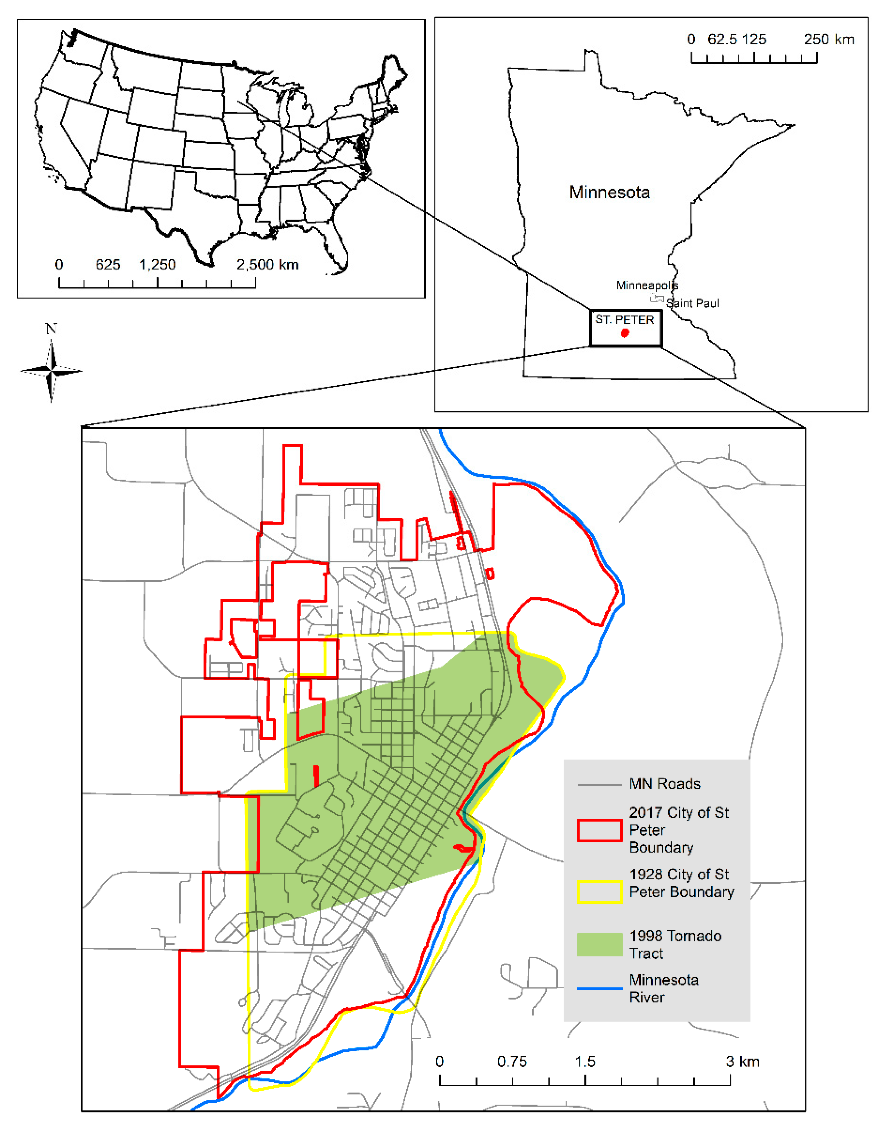
2.1. Study Site

The City of St Peter is situated in Nicollet County, 96 km south of the Minneapolis–Saint Paul Twin Cities, USA, with the Minnesota River on the east boundary and a bluff to the west (Figure 1). The coordinates of its central location are 44.323°N and 93.958°W. The total area of the City is 14.76 km2 with 11,400 residents [42]. The total boulevard tree population is 4824 trees. The majority of the population consists of 1414 maple (Acer spp.), 1094 ash (Fraxinus spp.) and other species such as 404 basswood (Tilia spp) and 301 hackberry (Celtis spp.) [43]. On March 29, 1998, between 17:18hrs and 17:36hrs, a tornado struck the city, and many of the town’s houses, businesses, civil buildings and urban forests were damaged. Therefore, one aspect of this study examined the impact of the 1998 tornado on the urban canopy cover area. The possibility of detecting forest canopy change due to the tree diseases Dutch Elm Disease (Ophiostoma ulmi and O. nova-ulmi) and Butternut Canker (Sirococcus clavigigenti-juglandacearum) was also explored, as hundreds of millions of trees have been infected since the 1960s in the USA.

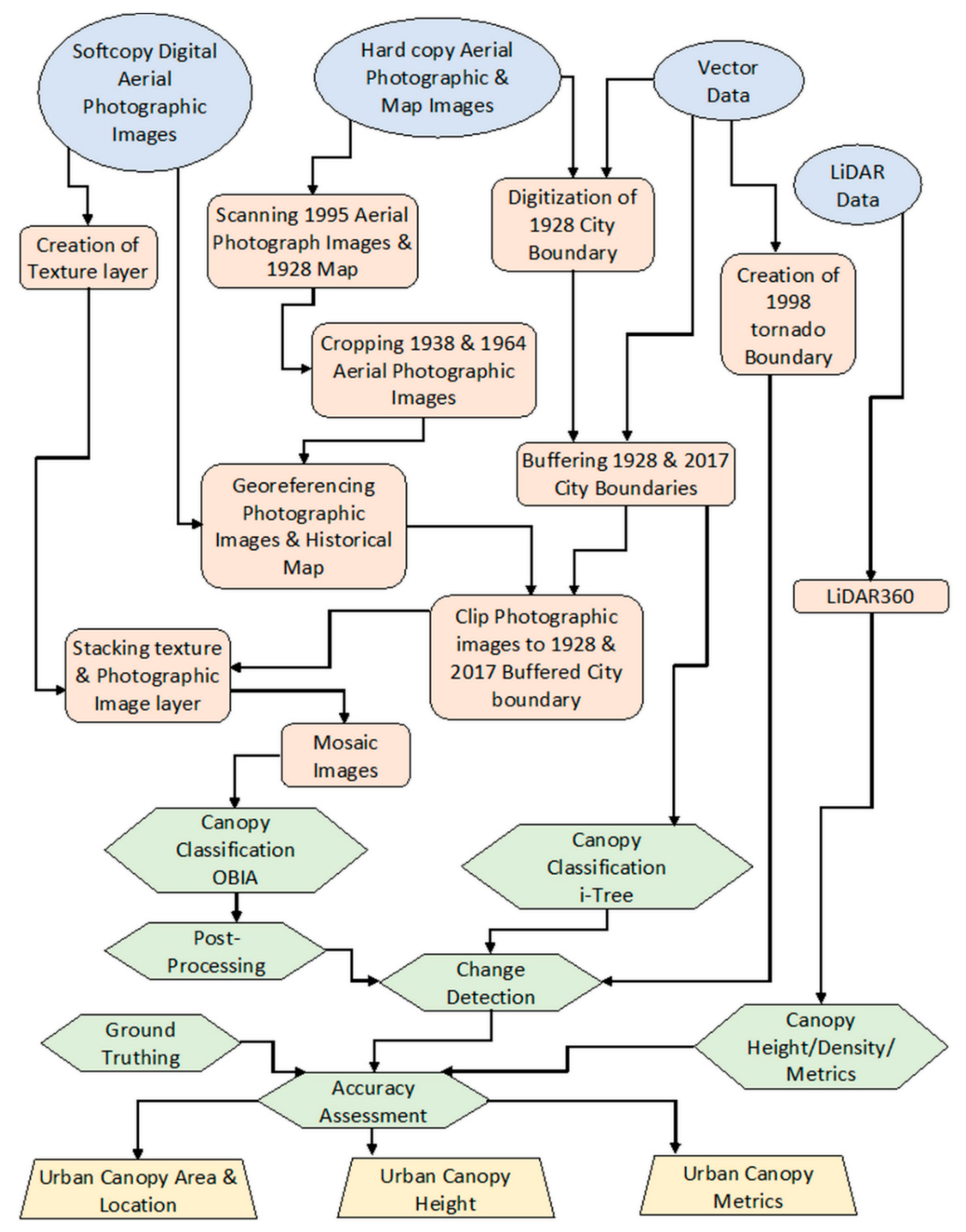
2.2. Data and Preprocessing

The complete methodological process, described in Section 2.2, Section 2.3, Section 2.4, Section 2.5 and Section 2.6, is shown as a schematic in Figure 2. The research data consisted of digital airborne ortho-images and aerial photographs, hardcopy historical aerial photographs, scanned images and historical maps, vector data, and LiDAR data. Table 1 and Table 2 provide detailed information regarding the multi-source datasets. Seven selection criteria determined the aerial images used: (1) high image resolution, i.e., 600 Dots Per Inch (DPI) or pixel resolution ≥ 0.93 m; (2) minimum map scale of 1:20,000; (3) trees with leaves on; (4) historical photographic images taken during the same months; (5) images with the full areas within the city boundary of 1928 and 2017; (6) ease of access to and availability of images; (7) images just prior to and post the 1998 tornado. The images selected were for 1938, 1951, 1964, 1995, 2008, and 2017 (Table 1).
To prepare the images, first, the 1938 and 1964 Black and White (B+W) panchromatic images were cropped to remove black borders and distorted sections of the image deemed unsuitable for analysis, e.g., incorrect tone. Second, the 1995 aerial image and the 1928 engineering map were transferred from hard copy to soft copy by digital scan (3-band, natural color at 600 DPI). Third, the 1938, 1951, 1964, and 1995 aerial photographic images lacked camera parameters and exterior orientation parameters [2] and could not be orthorectified. Therefore, the photographic images and the 1928 engineering map were georeferenced [2] within ArcGIS 10.6.
The root-mean-square errors (RMSEs) range from 1.40 m to 113.60 m; on average, 17 GCPs were used. The 1951 south image and 1928 engineering map (Table 3) had relatively high RMSEs; both were georeferenced with a first-order polynomial transformation. The 1928 GCPs were based on a reference photograph from 1951, due to difficulty in determining viable GCPs in 1938. The high RMSE is likely due to the limited GCPs available, which were based on the road layout; it is also probable that the road layout changed between 1928 and 1951. For example, the Saint Peter Broadway Bridge (highway 99) was remodeled three years after the 1928 engineering map [45]; therefore, the road layout detailed in 1951 may have changed accordingly. It should be noted that the process for accuracy of individual images was based on a compromise between both RMSE and visual interpretation due to the disparity in image type, location of suitable GCPs for overlapping and adjacent images, limited availability of GCP sites, and temporal variation of the photographic images when georeferencing. Therefore, low RMSEs do not guarantee high positional accuracy [46].
After georeferencing, the city limits were digitized and a polygon feature class created from the 1928 engineering map. The 1928 and 2017 feature class boundaries were buffered to 60.96 m for two reasons. First, the city boundary is a human construct and the urban forest does not conform to a linear boundary. Using visual estimation, it was determined that no trees in the boundary areas had a canopy width greater than 121.92 m; therefore, the 60.96-m buffer contained trees within the city boundary. Second, the 60.96-m boundary and the remaining minimum bounding rectangle with the 1928 and 2017 city boundary was a large enough area to perform validation results on the aerial photographic images. The 1998 tornado boundary was created by buffering two polyline shapefiles to a distance of 2.01 km, clipping them to the 1928 and 2017 boundary, reflecting the geographic extent of the tornado as described by the NOAA Storm Prediction Center’s (SPC) United States severe report database [47].
The aerial photographic images were clipped to the 1928 and 2017 city feature classes and a single raster dataset was created by mosaicking the clipped aerial photographic images. To aid distinction between land use classes for the B+W panchromatic and 1995 three-band color image, a 3 × 3 variance (second-order) texture layer was created from the mosaicked photographic images within ERDAS IMAGINE 2018 [48]. Each texture layer was stacked with the mosaicked photographic image.

2.3. OBIA Urban Forest Canopy Analysis and Change Detection

For analyzing high-resolution B+W panchromatic aerial photographs, texture can be crucial to maximize extraction of land use categories, particularly forest and urban forest areas [48,49,50]. B+W Panchromatic photographs have low radiometric and spectral information and texture adds another variable for extraction [48]. Feature Analyst, the software chosen for OBIA analysis, includes texture as an object input [51]; the combination of the texture layer created in ERDAS IMAGINE 2018 and that included within Feature Analyst gave the best results.
Feature Analyst uses a contextual classifier in its segmentation process which utilizes object size, edge type, spatial context, and shape to produce vector files that can be edited [51,52]. After preliminary investigations using this software, it became apparent that the extraction classification process was most effective if supervised learning using multiple classes (Table 4) was used rather than unsupervised or a single-class approach [53]. Large shrubs were included within the urban forest, as it is virtually impossible to differentiate between trees and large shrubs in the B+W panchromatic images due to the resolution and hue/tone. It also became apparent, as documented by Yuan [48], that differentiation between grass and soil in the B+W panchromatic images was challenging; the classes were combined as grass/soil. For consistency, these classes were kept for B+W panchromatic, three-band natural color, and four-band color infrared images. All the images had some form of shadow; therefore a shadow/other class was created as detailed in Qiu, Wu [54].
Training samples were manually digitized drawing close to the edge of class features (objects) to represent the shape, size, spectral content, texture, patterns, and contextual data and to distinguish them from adjacent objects [54,55]. Due to the differences between the three types of aerial photographic images, multiple supervised learning operations were repeated using different histogram stretches, learning options, and input representations to extract each class.
Post-processing of the OBIA data was performed first in ArcGIS by visibly comparing the OBIA canopy cover class polygons to the photographic images and removing inaccuracies. Second, the OBIA polygon was converted to raster and imported into ERDAS IMAGINE 2018, where a majority function using a 3 x 3 window was used to remove single pixels incorrectly classified as canopy cover.
To quantitatively determine and compare canopy change between the years, a post-classification change detection model was created within ERDAS IMAGINE 2018 [56]. The change detection model created a thematic layer from a matrix that evaluated two historical image files. This thematic layer displays the unique difference in the values of the two overlapping original images [57].

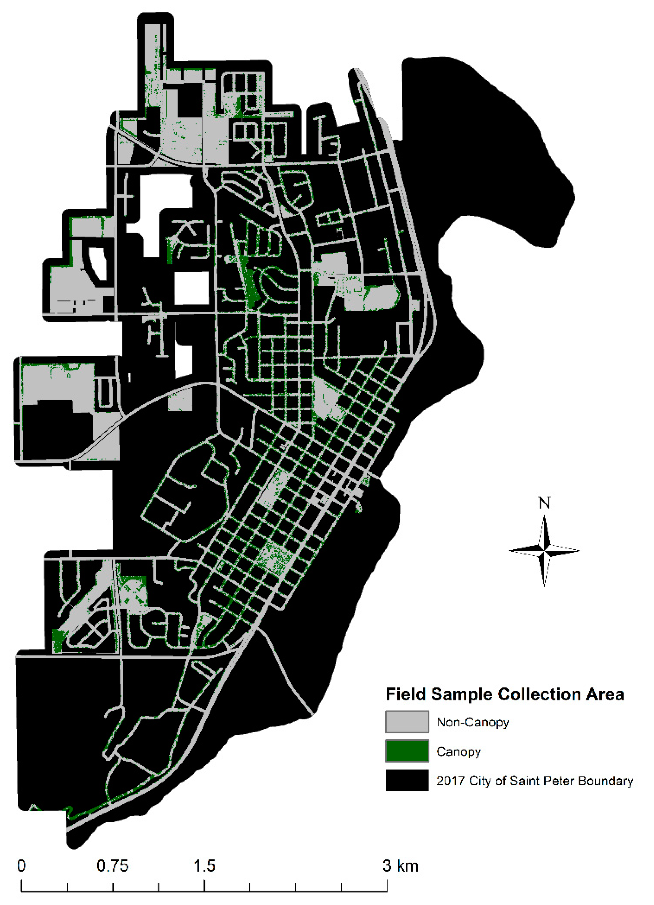
2.4. Accuracy Assessment of Urban Forest Canopy cover Extracted by OBIA

For accuracy assessment, a site-specific thematic error matrix [58] and Kappa coefficient were created, using the method proposed by Zhou and Troy [59]. Stratified random sampling enabled the canopy and non-canopy classes to be proportionately weighted; there were fewer canopy class features compared to non-canopy features and these were unevenly distributed [54]. To mitigate against potential positional inaccuracy, a small difference in cell size between photographic images of different years, and ensure a representative sample within a category polygon [58], a sample unit of a 5 × 5 pixel block was created for each year. Congalton and Green [58] state that when the research site is less than 404,686 hectares and 12 classes, a minimum of 50 samples per class is needed for accuracy assessment. Therefore, 150 samples were used: 50 per class (forest, non-forest) and 50 randomly distributed. As no higher-resolution images were available for reference data, the same high-spectral-resolution aerial photographic images were used for the accuracy assessment process. Field sample collection was possible for the 2017 dataset. The area selected for field sample data was based on the ability to legally and practically assess areas within the 2017 city boundary: the city owned land (parcel) and the rights of way (ROW) of all roads within the city boundary (Figure 3).
The field sampling map was created in ArcGIS by buffering the Nicollet County streets shapefile to reflect the correct ROW distance for streets within the city, dependent on municipal code. This dataset was merged with the city tax parcel polygon shapefile. Any significant difference between the 2017 photographic image and 2019 ground truthing was mitigated by the researcher’s in-depth knowledge as the city’s urban forester.

2.5. Urban Forest Canopy Cover Assessment Using i-Tree Canopy

i-Tree is a freely available suite of urban forest ecosystem service evaluation software, created by the U.S. Forestry Service and other collaborators [60,61]. i-Tree Canopy is one tool within i-Tree that allows users to define land cover categories (e.g., water, trees) using a web browser application (Google Maps and Google Earth) to enable photo interpretation of current and historical aerial imagery using randomly selected points [62]. The Google Maps 2019 image and the Google Earth 2008 image were selected for their relevance.
Both 1928 and 2017 polygon boundary shapefiles were imported into i-Tree Canopy and five classes, as per OBIA, were created. Employing the 2019 Google photographic image in Google Maps; one thousand randomly generated survey points were produced, and, through photo-interpretation, each point was assigned a class, as recommended by the i-Tree Canopy technical notes [63]. To photo-interpret the 2008 Google Earth image, a Keyhole Markup Language (KML) file, representing the randomly generated survey points produced for the 2019 images, was imported into Google Earth. Using the 2008 Google Earth photographic image, each imported point was photo-interpreted and assigned a class.

2.6. Urban Forest Metrics Detection Using LiDAR

LiDAR data was analyzed with LiDAR360 software [64]. To improve data’s quality, LiDAR data preprocessing included reclassifying the point cloud and removing outliers. LiDAR360 can re-classify by machine learning, using a small training sample that was manually corrected to reclassify points and then using the random forest method along with the training sample to edit the entire dataset in batches [64]. Initial results were poor; therefore, the following three LiDAR point classification processes were applied and proved successful. First, bare earth ground points were classified/reclassified using the improved progressive TIN densification filtering algorithm proposed by GreenValley International Ltd [64], Zhao, Guo [65]. The maximum building size was set to 160 m, the actual length of the largest building within the study site. Second, the bare earth ground points were refined by fitting quadratic surfaces using a concoid filter [64]. The point cloud was classified, paying particular attention to the vegetation points using the interactive editing module, which allows the user to manually edit points or groups of points with a profile tool. Finally, to remove topographic relief elevation effects, the LiDAR points were normalized by subtracting the closest classified bare earth ground point elevation from other classified points’ z value [64].
To create a canopy height model (CHM), a Spike Free TIN method [64,65] was used to interpolate a Digital Surface Model (DSM) and a Digital Elevation Model (DEM). Medium vegetation returns were used instead of first returns to improve accuracy by removing buildings, etc., which in an urban environment can be higher than the urban canopy. The CHM was created by subtracting the DSM from the DEM. Canopy cover density was determined by calculating the ratio of medium vegetation returns to the total number of LiDAR first returns for a pixel [64]. Vegetation below 2 m was removed, and the pixel size was determined by measuring the width of the largest single tree canopy, 33 m.
Two different tree segmentation models—CHM segmentation and the point cloud segmentation model—were used to determine individual tree attributes, e.g., tree location, height, crown diameter, crown area and volume. In CHM segmentation, watershed segmentation recognizes and demarcates individual tree crowns using the CHM created in the previous step as the input layer. The watershed segmentation algorithm inverts individual tree canopy points to represent a catchment basin. The level at which the water would start to overflow the basin represents the bottom of the individual tree canopy [64,66]. From this segmentation, tree location, height, crown diameter, and crown area can be calculated. Point cloud segmentation uses the relative spacing between trees. As spacing at the top of trees is greater than at the bottom, LiDAR points are included or excluded based on their relative distance to each other, starting at the top of the tree and working down. Using this segmentation process, the same tree attributes were created [12,64]. To extract tree metrics, a normalized point cloud consisting of vegetation points was created, and, due to the close proximity of trees in areas within the research site, the spacing threshold was set to 0.5 m.

3. Results

3.1. Accuracy Assessment of OBIA and Stratified Random Sampling Results

In general, for OBIA (Table 5), the overall classification accuracy was excellent: over 90% except 1995 (89.33%). The overall Kappa statistics show strong agreement (>80%) [58] between the years, excepting 1995 (0.78%). In general, the error matrix shows that the producer’s accuracy for canopy (89%–97%) is higher than the user’s accuracy (84%–94%), excepting the 2017 OBIA (1928 boundary). The error matrices for the entire period 1938–2017 show that the producer’s accuracy (89%–97%) (omission error) of canopy cover ranges from 3% to 11%; slightly higher than user’s accuracy (84%–94%) (commission error) of 16% to 6%, excepting the 2017 OBIA (1928 boundary) (Table 5). However, different producer’s and user’s accuracies were obtained using the 2017 city boundary. Therefore, accuracy assessment results appear sensitive to the study site boundary. To enhance the OBIA accuracy assessment validation, ground truthing was conducted. Due to only being able to access public property combined with local flooding, the area available to ground truth within the city was approximately ¼ of the total 2017 boundary. Despite these restrictions, the error matrix is comparable to those within photointerpretation (Table 5).
Using standard error (SE), i-Tree’s stratified random sampling has a 95% confidence interval for 2008 and 2019 canopy cover data (1928 boundary) of + or – 1.45, leading to a 31.75%–28.85% canopy cover estimation, in 2008, and 1.53, equating to a 38.33%–35.27% canopy cover estimation, in 2019. For the 2019 data (2017 boundary), 31.86%–28.94% canopy cover change was estimated, as the SE is + or – 1.46 (Table 6).

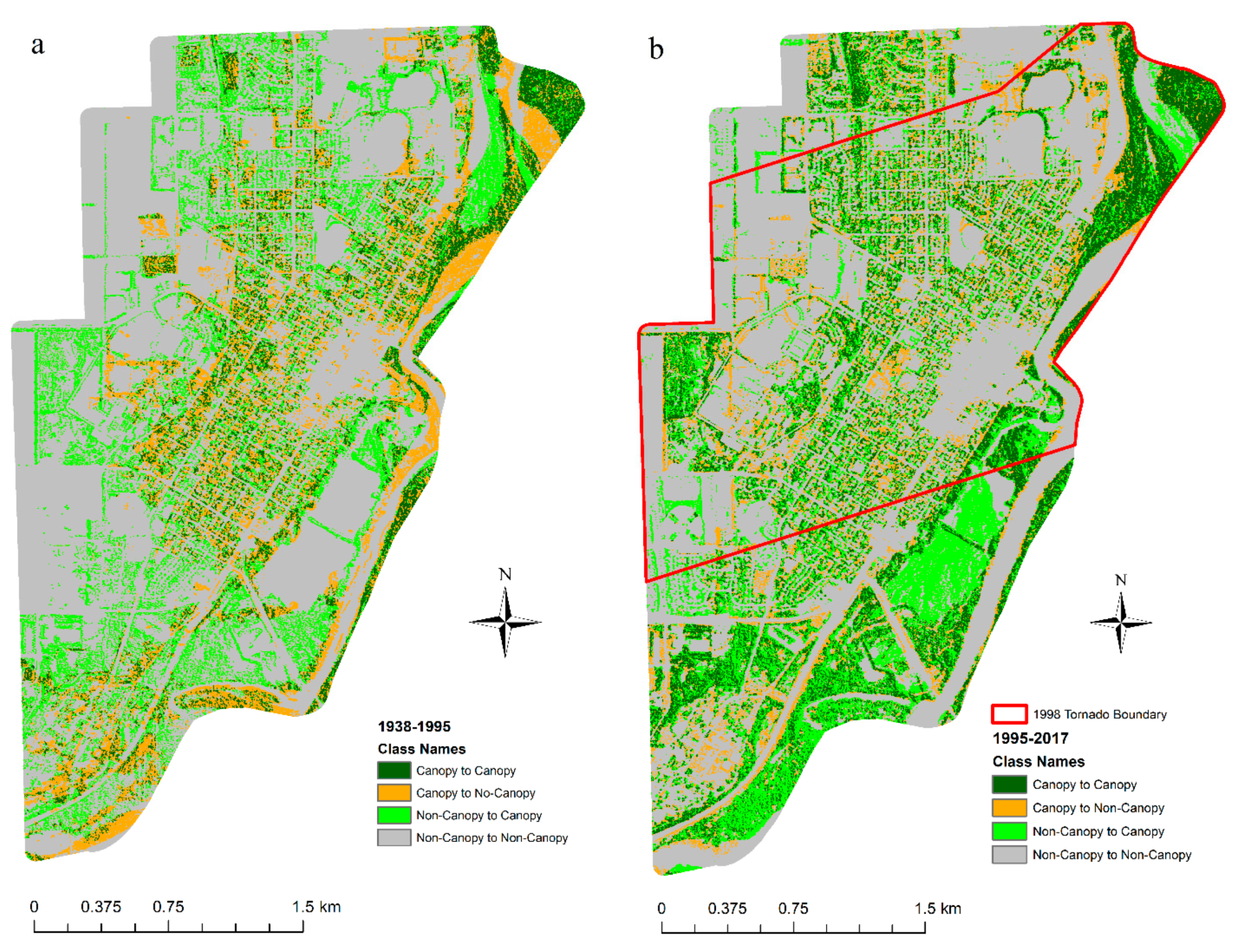
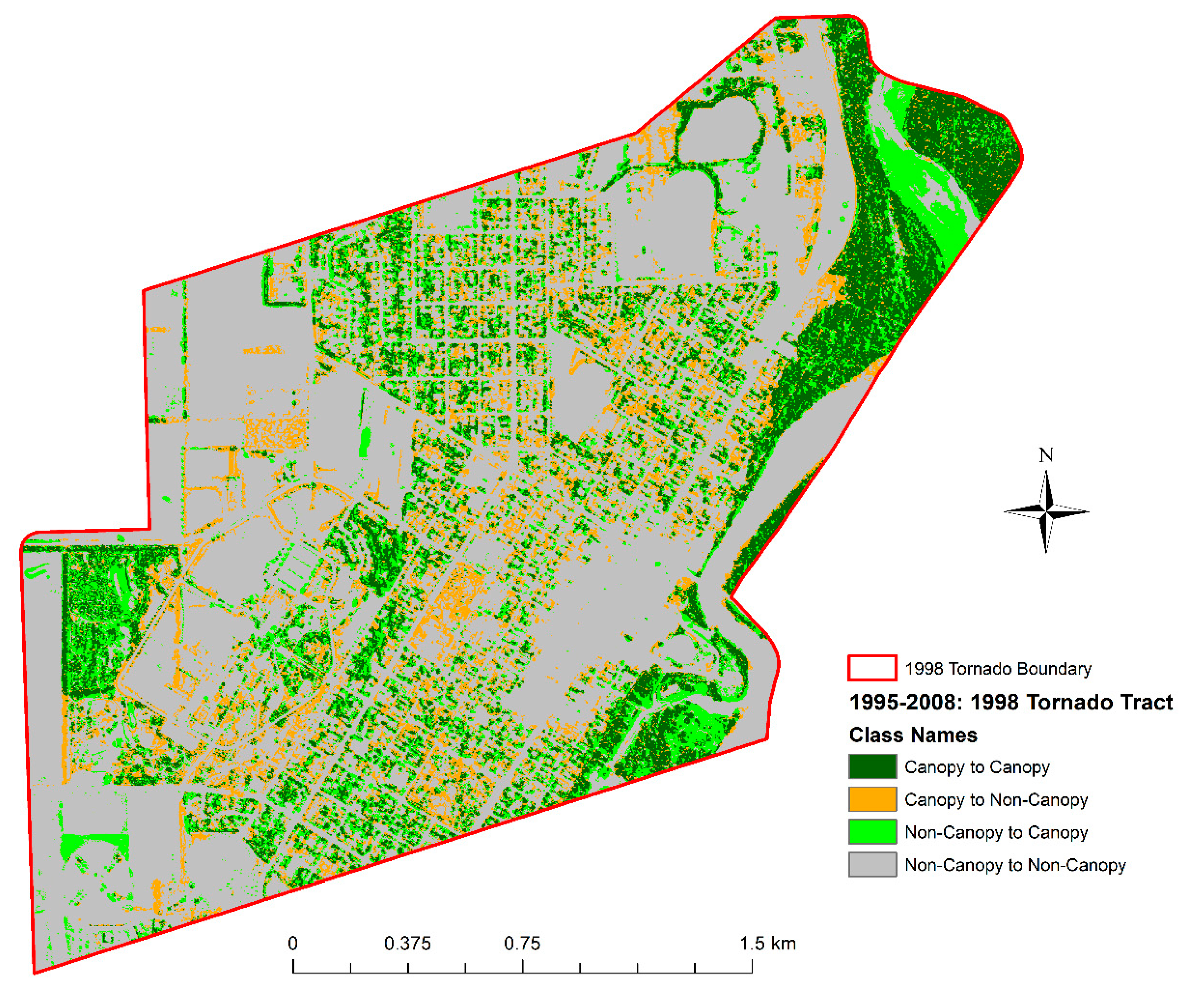
3.2. Trend of Urban Forestry Canopy Change and the Impacts of the 1998 Tornado and Tree Diseases

For the 1928 City boundary, the OBIA analytical results (Table 7) show a general trend of canopy increase from 1938 to 2017, with a minimum area in 1938 of 20.68% to a maximum of 35.53% in 2008. Total canopy area can be split into two specific time frames: pre-1995 and post-1995. Pre-1995 % area ranges from 20.68% (1938) to 25.97% (1995); post-1995% area ranges from 35.53% (2008) to 35.30% (2017).
i-Tree’s stratified random sampling confirms that from 2008 to 2019 the percentage canopy cover within the 1928 boundary is ~ 30%–35% (Table 6). From 1938 to 1995 (57 years), canopy cover increased as a proportion of city area by 5%. From 1995 to 2017 (22 years), canopy cover increased by 10% of the city area. In fact, the 10% increase occurred between 1995 and 2008 and canopy cover remained stable from 2008 to 2019.
The canopy change map (Figure 4) shows that between 1938–1995 and 1995–2017 the majority of canopy increase took place on the east boundary of the city along the Minnesota River flood plain, within the central urban areas, e.g., streets and backyards and towards the north, west, and south boundary edges of the city. The increase in canopy area along the river flood plain is due to a change in land management; areas shifted from farmland to naturalized woodland. The tornado response is primarily responsible for the increase in the central urban reforestation. Canopy cover increased towards the edges of the city boundary, as new development of previous farmland created new areas for planting trees. While overall canopy cover increased, many areas remained non-canopy areas, or changed to non-canopy, primarily before 1995. The change to non-canopy is particularly evident along the Minnesota River flood plain between 1938–1951 and 1964–1995, where the shift in the river’s position and subsequent flooding have changed the land use. Within the city center, areas have changed to non-canopy, likely due to redevelopment, e.g., dividing a large parcel containing one property and trees into smaller parcels containing fewer trees.
The canopy change between 1995 and 2008 within the tornado tract (Figure 5) shows increased canopy cover on streets and backyards, as well as along the Minnesota River flood plain. The canopy to non-canopy area change during this time span is primarily due to the tornado, as these areas have changed due to infrastructure conversion or redevelopment, e.g., houses, parking lots. The results of this study reveal that more than 45% of the canopy cover within the defined F3 tornado (158–206mph) boundary was lost.
The butternut (Juglans cinerea L.) and, particularly, the American elm (ulmus americana L) trees were both highly visible within the urban forest and naturalized areas prior to the 1980s, but due to Dutch Elm Disease and Butternut Canker they have disappeared, excepting a few disease-resistant “survivor” trees. Due to a probable combination of image resolution and the length of time between images it was not possible to determine any correlation between the loss of these tree species and canopy cover. However, up until 1995, canopy cover remained relatively constant, therefore replanting using other tree species, e.g., maple (Acer spp.), or natural regrowth mitigated the loss.
The results primarily focused on the 1928 city boundary. However, comparing the 1928 (941 hectares) and 2017 (1705 hectares) city boundary data for canopy cover for both OBIA and random sampling for the years 2008 and 2017/19, the data shows that the areas have a comparable canopy cover of ~34%, even though the 2017 area is almost double that of the 1928 boundary.

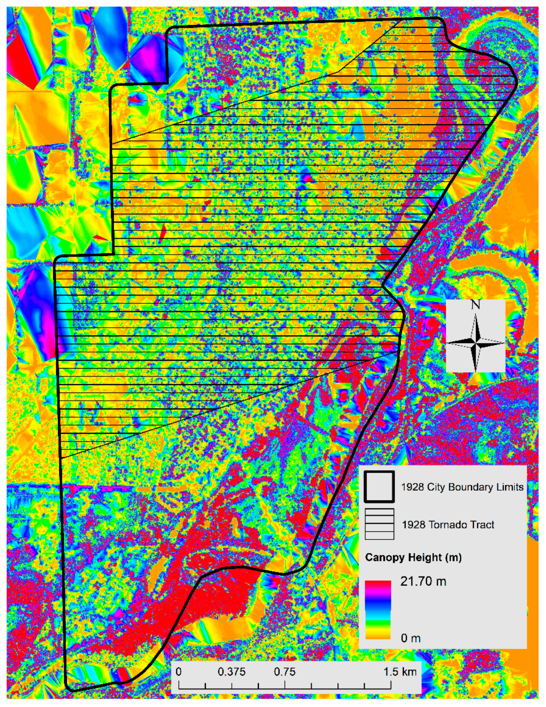
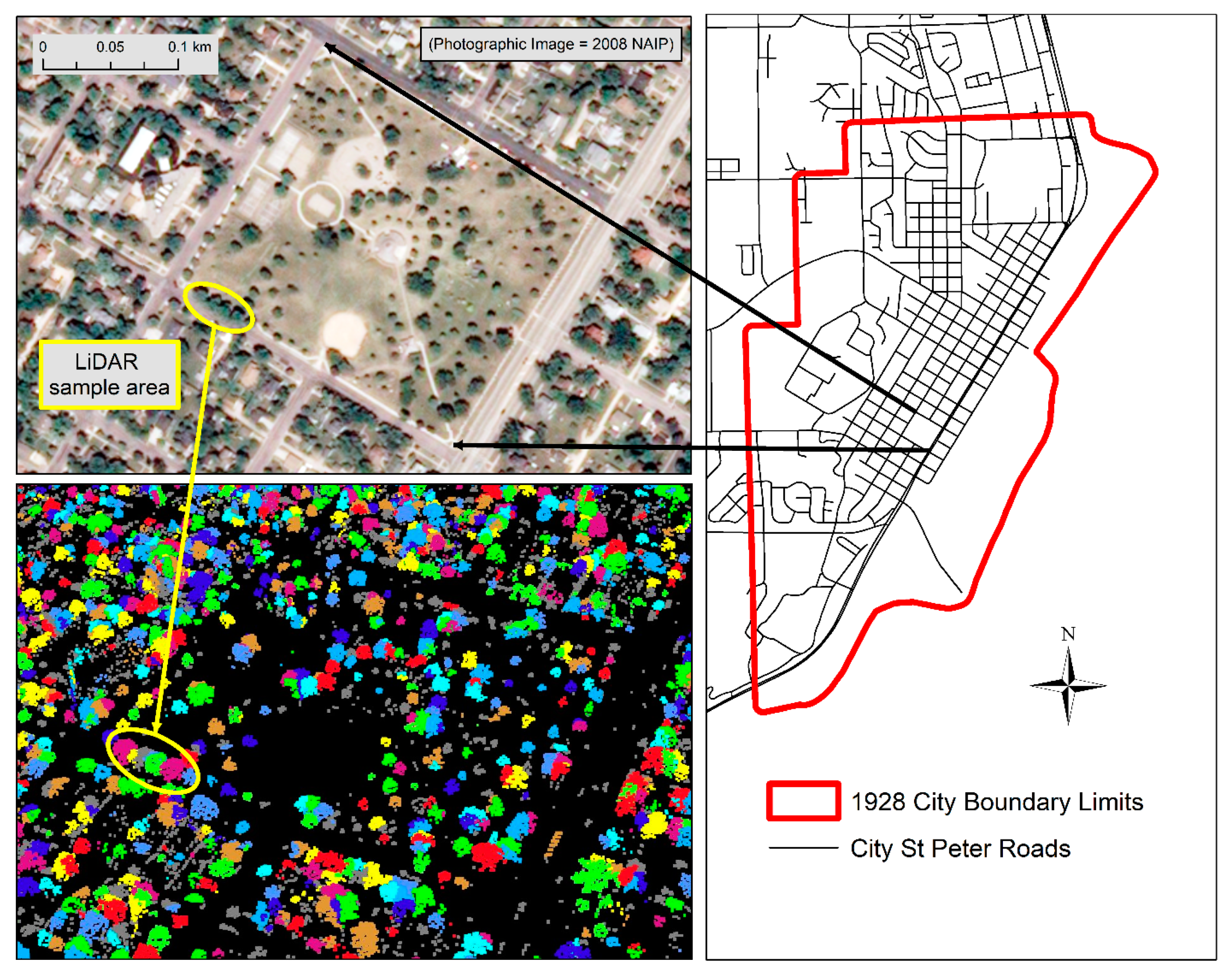
3.3. Urban Forest Canopy Density, Height Assessment and Individual Tree Metrics using LiDAR

LiDAR was used to create a canopy cover density model, CHM, and tree metrics for 2010. The canopy cover model shows the total canopy coverage within a pixel area of 10.06 m2. Although the resolution of canopy coverage is low compared to the OBIA 2008 data (0.28 m2), the two datasets corroborate each other with respect to canopy cover (Figure 6).
Figure 7 shows canopy cover height. The majority of the highest canopy and tallest trees are in naturalized areas within the flood plain (>12.19m), which is expected due to environmental conditions, e.g., soil, nutrients, water allocation, etc., allowing extended growth of pioneer species specific to the environment, such as poplar (e.g. Populus deltoides). Isolated areas of high canopy within the city center are trees that survived the tornado. The path of the tornado through the city (Figure 7) is visible, as is the lower height of the canopy within the tornado tract compared to the canopy height north and south of the tornado boundary. The high canopy located on the west boundary in the flood plain is due to the density of trees protecting them from wind exposure as compared to isolated individual trees within the urban environment.
The tree attributes determined for both the Canopy Height Model (CHM) and point cloud (PC) segmentation processes were tree location, tree height, crown diameter, and crown area. The point cloud segmentation process also provided crown volume. However, both processes extracted a different number of trees. Table 8 shows a selection of tree attributes for trees located along the south west corner of Minnesota Square Park (Figure 8). Both the x and y tree locations are accurate. However, the remaining metrics each have accuracy discrepancies and cannot be rectified without performing regression analysis, not included within this study.

4. Discussion

4.1. Comparision of the Urban Canopy Cover Assessment Methods and Factors of Urban Canopy Cover Changes

The accuracy assessment results of the OBIA and the random-point-based sampling methods (Table 5 and Table 6) indicate that both analysis techniques are accurate enough to assess urban canopy cover change based on high-spatial-resolution remote sensing images. The difference in results may be partially attributed to a difference in image quality and resolution, e.g., Google imagery compared to NAIP imagery [63]. Whilst comparable, i-Tree random-point-based assessment only shows the total coverage of the classes and cannot detail the locations of canopy change over time; however, the stratified random sampling technique is quick, taking days to complete compared to weeks for OBIA. In addition, a possible answer for the lower classification accuracy for 1995 based on the OBIA (Table 5) is that the 1995 photographic image has relatively low spectral variability even though it was scanned at a high spatial resolution. Because the digitally scanned image is essentially a copy of the hardcopy photograph, not the original negative, spectral information can be lost during the scanning process, according to Feature Analyst’s product support lead, William Veteto.
Natural disasters, urban development, and the shift of the Minnesota River channel are the main factors for urban forest cover change in this study area. The 1998 tornado caused considerable damage to both grey and green infrastructure. As mentioned in Section 3.2, a minimum of 45% of the canopy cover within the tornado tract was lost between 1995 and 2008. After the tornado, the City implemented a tree replanting regime. Forty percent of the planting occurred within the tornado tract, with 60% planted in remaining areas of the city. Replanting led to a 10% increase in canopy cover by 2008, especially in the central urban area, and led to a total canopy cover of 35% that has since remained stable. Changes in land management (e.g., farmland converted to naturalized woodland) led to the increase in canopy area along the river flood plain. Urban canopy change to non-canopy within the city center areas could also be attributed to urban redevelopment. The shift in the river’s position and subsequent flooding have caused an evident change to non-canopy along the Minnesota River flood plain between 1938–1951 and 1964–1995. Nevertheless, due to the limitations of the spectral and temporal resolutions of the images used in this study, it was not possible to determine the canopy cover change caused by tree diseases.

4.2. Limitations and Potentials of Canopy Metrics Extraction using LiDAR Data Analysis

Except for tree locations, the other canopy metrics determined for both CHM and PC segmentation processes based on the LiDAR data demonstrated remarkable discrepancies (Table 8). For example, tree heights for both processes vary by 0.91–2.43 m. For crown diameter and crown area, the differences are even greater between processes, e.g., for the same tree crown diameter (CHM 25.76 m vs. point cloud 38.98 m) and crown area (CHM 521.28 m2 vs. point cloud 1193.32 m2). These canopy metrics’ accuracy is limited by several factors. Firstly, the research LiDAR was collected with the leaves off; forestry research LiDAR is typically collected with the leaves on. Secondly, the LiDAR point cloud was 0.08 points/m2, 2.25 times less dense than the minimum commonly used within LiDAR-derived forest research, 0.18 points/m2 [12,66,67]. Thirdly, after improvement of the LiDAR data quality, errors remained in the point cloud classification and therefore there is the potential to locate trees where none exist. More detailed information about this can be found in Blackman [68]. Fourthly, LiDAR360 offers only one algorithm for CHM segmentation, based on a paper that uses an algorithm where the research location is oak savannah woodland, not an urban forest. The only building structure was a fire lookout, removed from the data prior to the assessments [66]. Likewise, there is only one point cloud segmentation algorithm provided by LiDAR360 software based on a previous study that uses a segmentation algorithm where the research area is a mixed conifer forest, not an urban environment [12]. In conclusion, the canopy metrics analysis is limited by the quality of the publicly available LiDAR data and the limitations of the LiDAR data processing software.

5. Conclusions

This paper has shown the importance of remote sensing techniques to extract invaluable information from historical data sources. It demonstrated that both the OBIA and the point-based non-image classification approach could determine the temporal change in the canopy cover accurately from historical aerial images. The point-based random sampling method is an efficient method to determine the urban forest canopy cover area but lacks locational information. In contrast, the OBIA offers the ability to ascertain spatial-temporal canopy change leading to more detailed analysis, but this can be time-consuming and requires specialist knowledge. Based on this research, urban forest stakeholders can now choose whether to use OBIA or random-point-based assessment to determine urban tree canopy cover dependent on their specific purposes.
The post-classification comparison change analysis indicated that the 1998 tornado had the largest impact on canopy cover changes in the study site in addition to the other two identified factors —urban development and the shift of the Minnesota River channel. However, tree disease impact on canopy cover was undetectable in the OBIA-based classification maps derived from the historical aerial images. This might be partially attributed to a limitation of the study—only having access to hard-copy historical images acquired in some discrete years but lacking access to digital multi-spectral airborne images with high spectral and temporal resolutions.
The research also revealed the value and potential of LiDAR data and techniques to determine urban forest metrics. However, the canopy metrics analysis in this study is limited by the quality of the freely available LiDAR data and the limitations of the LiDAR data processing software. To accurately extract canopy metrics (such as crown area, diameter, and volume) in addition to locations of urban canopies, more dense LiDAR point cloud data collected during the leaf-on season, sample and independent variable data, as well as LiDAR processing software with algorithms developed specifically for urban forest analysis are needed.

Author Contributions

Conceptualization, R.B.; methodology, R.B. and F.Y.; software, R.B.; validation, R.B.; formal analysis, R.B.; investigation, R.B.; resources, R.B.; data curation, R.B.; writing—original draft preparation, R.B.; writing—review and editing, R.B. and F.Y..; visualization, R.B.; supervision, F.Y.; project administration, R.B.; funding acquisition, R.B. All authors have read and agreed to the published version of the manuscript.

Funding

This research was funded by the Minnesota State University, Mankato’s, 2019–2020 James F. Goff Graduate Research Award and the 2019–2020 Dr. Mary Dooley Scholarship Award.

Conflicts of Interest

The authors declare no conflict of interest. The funders had no role in the design of the study; in the collection, analyses, or interpretation of data; in the writing of the manuscript; or in the decision to publish the results.

References

  1. Grant, S. The Right Tree in the Right Place: Using GIS to Maximize the Net Benefits from Urban Forests, in Physical Geography and Ecosystem Science. Master’s Thesis, Lund University, Lund, Sweden, 2015; p. 63. [Google Scholar]
  2. Wright, J.; Lillesand, T.M.; Kiefer, R.W. Remote Sensing and Image Interpretation. Geogr. J. 1980, 146, 448. [Google Scholar] [CrossRef]
  3. Ward, K.T.; Johnson, G.R. Geospatial methods provide timely and comprehensive urban forest information. Urban For. Urban Green. 2007, 6, 15–22. [Google Scholar] [CrossRef]
  4. Hawthorne, T.L.; Elmore, V.; Strong, A.; Bennett-Martin, P.; Finnie, J.; Parkman, J.; Harris, T.; Singh, J.; Edwards, L.; Reed, P. Mapping non-native invasive species and accessibility in an urban forest: A case study of participatory mapping and citizen science in Atlanta, Georgia. Appl. Geogr. 2015, 56, 187–198. [Google Scholar] [CrossRef]
  5. Nowak, D.J.; Rowntree, R.A.; McPherson, E.; Sisinni, S.M.; Kerkmann, E.R.; Stevens, J.C. Measuring and analyzing urban tree cover. Landsc. Urban Plan. 1996, 36, 49–57. [Google Scholar] [CrossRef] [Green Version]
  6. Thenkabail, A.; Lyon, P.; Huete, J. Hyperspectral Remote Sensing of Vegetation; Hyperspectral Remote Sensing of Vegetation; CRC Press: Boca Raton, FL, USA, 2016; p. 705. [Google Scholar]
  7. Voss, M.; Sugumaran, R. seasonal effect on tree species classification in an urban environment using hyperspectral data, LiDAR, and an object-oriented approach. Sensors 2008, 8, 3020–3036. [Google Scholar] [CrossRef] [Green Version]
  8. Knight, J.; Host, T.; Rampi, L. 2015 Urban Tree Canopy Assessment Twin Cities Metropolitan Area; Department of Forest Resources, University of Minnesota: St. Paul, MN, USA, 2016; pp. 1–15. [Google Scholar]
  9. Hovi, A.; Korhonen, L.; Vauhkonen, J.; Korpela, I. LiDAR waveform features for tree species classification and their sensitivity to tree- and acquisition related parameters. Remote Sens. Environ. 2016, 173, 224–237. [Google Scholar] [CrossRef]
  10. Sumnall, M.J.; Hill, R.A.; Hinsley, S.A. Comparison of small-footprint discrete return and full waveform airborne lidar data for estimating multiple forest variables. Remote Sens. Environ. 2016, 173, 214–223. [Google Scholar] [CrossRef] [Green Version]
  11. Yao, W.; Krzystek, P.; Heurich, M. Tree species classification and estimation of stem volume and DBH based on single tree extraction by exploiting airborne full-waveform LiDAR data. Remote Sens. Environ. 2012, 123, 368–380. [Google Scholar] [CrossRef]
  12. Li, W.; Guo, Q.; Jakubowski, M.K.; Kelly, M. A New Method for Segmenting Individual Trees from the Lidar Point Cloud. Photogramm. Eng. Remote Sens. 2012, 78, 75–84. [Google Scholar] [CrossRef] [Green Version]
  13. Zhang, C.; Zhou, Y.; Qiu, F. Individual Tree Segmentation from LiDAR Point Clouds for Urban Forest Inventory. Remote Sens. 2015, 7, 7892–7913. [Google Scholar] [CrossRef] [Green Version]
  14. Zhen, Z.; Quackenbush, L.; Zhang, L. Trends in Automatic Individual Tree Crown Detection and Delineation—Evolution of LiDAR Data. Remote Sens. 2016, 8, 333. [Google Scholar] [CrossRef] [Green Version]
  15. Lindberg, E.; Holmgren, J. Individual tree crown methods for 3D data from remote sensing. Curr. For. Rep. 2017, 3, 19–31. [Google Scholar] [CrossRef] [Green Version]
  16. Shrestha, R.; Wynne, R. Estimating Biophysical Parameters of Individual Trees in an Urban Environment Using Small Footprint Discrete-Return Imaging Lidar. Remote Sens. 2012, 4, 484–508. [Google Scholar] [CrossRef] [Green Version]
  17. Plowright, A.A.; Coops, N.C.; Eskelson, B.N.; Sheppard, S.R.; Aven, N.W. Assessing urban tree condition using airborne light detection and ranging. Urban For. Urban Green. 2016, 19, 140–150. [Google Scholar] [CrossRef]
  18. Song, Y.; Imanishi, J.; Sasaki, T.; Ioki, K.; Morimoto, Y. Estimation of broad-leaved canopy growth in the urban forested area using multi-temporal airborne LiDAR datasets. Urban For. Urban Green. 2016, 16, 142–149. [Google Scholar] [CrossRef]
  19. Fujita, T.T. Proposed Characterization of Tornadoes and Hurricanes by Area and Intensity; Satellite and Mesometeorology Research Project, Department of the Geophysical Sciences, The University of Chicago: Chicago, IL, USA, 1971; pp. 1–46. [Google Scholar]
  20. Burgess, D.; Ortega, K.; Stumpf, G.; Garfield, G.; Karstens, C.; Meyer, T.; Smith, B.; Speheger, D.; LaDue, J.; Smith, R.; et al. 20 May 2013 Moore, Oklahoma, Tornado: Damage Survey and Analysis. Weather. Forecast. 2014, 29, 1229–1237. [Google Scholar] [CrossRef]
  21. Bloniarz, D.V.; Brooks, R.T. Preliminary Assessment of the Tornado Effects on Residential Street Canopy Cover, Temperature, and Humidity; USDA Forest Service, Northern Research Station: Madison, WI, USA, 2011; p. 6.
  22. Karstens, C.D.; Gallus, W.A.; Lee, B.D.; Finley, C.A. Analysis of tornado-induced tree fall using aerial photography from the Joplin, Missouri, and Tuscaloosa–Birmingham, Alabama, Tornadoes of 2011. J. Appl. Meteorol. Clim. 2013, 52, 1049–1068. [Google Scholar] [CrossRef] [Green Version]
  23. Yuan, M.; Dickens-Micozzi, M.; Magsig, M.A. Analysis of Tornado Damage Tracks from the 3 May Tornado Outbreak Using Multispectral Satellite Imagery. Weather. Forecast. 2002, 17, 382–398. [Google Scholar] [CrossRef]
  24. Gokaraju, B.; Turlapaty, A.C.; Doss, D.A.; King, R.L.; Younan, N.H. Change detection analysis of tornado disaster using conditional copulas and Data Fusion for cost-effective disaster management. In Proceedings of the 2015 IEEE Applied Imagery Pattern Recognition Workshop (AIPR), Washington, DC, USA, 13–15 October 2015; pp. 1–8. [Google Scholar] [CrossRef]
  25. Kingfield, D.; De Beurs, K.M. Landsat identification of tornado damage by land cover and an evaluation of damage recovery in forests. J. Appl. Meteorol. Clim. 2017, 56, 965–987. [Google Scholar] [CrossRef]
  26. Mercader, R.; Siegert, N.W.; Liebhold, A.M.; McCullough, D.G. Dispersal of the emerald ash borer, Agrilus planipennis, in newly-colonized sites. Agric. For. Èntomol. 2009, 11, 421–424. [Google Scholar] [CrossRef]
  27. Mercader, R.; Siegert, N.W.; Liebhold, A.M.; McCullough, D.G. Simulating the effectiveness of three potential management options to slow the spread of emerald ash borer (Agrilus planipennis) populations in localized outlier sites. Can. J. For. Res. 2011, 41, 254–264. [Google Scholar] [CrossRef]
  28. McCullough, D.G.; Mercader, R. Evaluation of potential strategies to SLow Ash Mortality (SLAM) caused by emerald ash borer (Agrilus planipennis): SLAM in an urban forest. Int. J. Pest Manag. 2012, 58, 9–23. [Google Scholar] [CrossRef]
  29. Mullen, K.; Yuan, F.; Mitchell, M. The Mountain pine beetle epidemic in the Black Hills, South Dakota: The consequences of long term fire policy, climate change and the use of remote sensing to enhance mitigation. J. Geogr. Geol. 2018, 10, 69. [Google Scholar] [CrossRef]
  30. Moskal, L.M.; Styers, D.M.; Halabisky, M. monitoring urban tree cover using object-based image analysis and public domain remotely sensed data. Remote Sens. 2011, 3, 2243–2262. [Google Scholar] [CrossRef] [Green Version]
  31. Hussain, M.; Chen, D.M.; Cheng, A.; Wei, H.; Stanley, D. Change detection from remotely sensed images: From pixel-based to object-based approaches. ISPRS J. Photogramm. Remote Sens. 2013, 80, 91–106. [Google Scholar] [CrossRef]
  32. Li, X.; Shao, G. Object-based land-cover mapping with high resolution aerial photography at a county scale in Midwestern USA. Remote. Sens. 2014, 6, 11372–11390. [Google Scholar] [CrossRef] [Green Version]
  33. Yu, Q.; Gong, P.; Clinton, N.; Biging, G.; Kelly, M.; Schirokauer, D. Object-based detailed vegetation classification with airborne high spatial resolution remote sensing imagery. Photogramm. Eng. Remote Sens. 2006, 72, 799–811. [Google Scholar] [CrossRef] [Green Version]
  34. Meneguzzo, D.M.; Liknes, G.C.; Nelson, M.D. Mapping trees outside forests using high-resolution aerial imagery: A comparison of pixel- and object-based classification approaches. Environ. Monit. Assess. 2012, 185, 6261–6275. [Google Scholar] [CrossRef]
  35. Pu, R.; Landry, S.; Yu, Q. Assessing the potential of multi-seasonal high resolution Pléiades satellite imagery for mapping urban tree species. Int. J. Appl. Earth Obs. 2018, 71, 144–158. [Google Scholar] [CrossRef]
  36. Walker, J.S.; Briggs, J.M. An Object-oriented Approach to Urban Forest Mapping in Phoenix. Photogramm. Eng. Remote Sens. 2007, 73, 577–583. [Google Scholar] [CrossRef]
  37. Hay, G.; Castilla, G. Geographic Object-Based Image Analysis (GEOBIA): A New Name for a New Discipline; Springer Science and Business Media: Berlin, Germany, 2008; pp. 75–89. [Google Scholar]
  38. Blaschke, T. Object based image analysis for remote sensing. ISPRS J. Photogramm. Remote Sens. 2010, 65, 2–16. [Google Scholar] [CrossRef] [Green Version]
  39. Nowak, D.J.; Hoehn, R.E.; Bodine, A.R.; Greenfield, E.J.; O’Neil-Dunne, J. Urban forest structure, ecosystem services and change in Syracuse, NY. Urban Ecosyst. 2013, 19, 1455–1477. [Google Scholar] [CrossRef]
  40. Strunk, J.; Mills, J.R.; Ries, P.D.; Temesgen, H.; Jeroue, L. An urban forest inventory and analysis investigation in Oregon and Washington. Urban For. Urban Green. 2016, 18, 100–109. [Google Scholar] [CrossRef] [Green Version]
  41. Bodnaruk, E.; Kroll, C.; Yang, Y.; Hirabayashi, S.; Nowak, D.; Endreny, T. Where to plant urban trees? A spatially explicit methodology to explore ecosystem service tradeoffs. Landsc. Urban Plan. 2017, 157, 457–467. [Google Scholar] [CrossRef] [Green Version]
  42. City of Saint Peter Statistics. Available online: https://www.saintpetermn.gov (accessed on 19 April 2017).
  43. City of Saint Peter. Species Distibution of Public Trees; Saint Peter, Ed.; City of Saint Peter: ST PETER, MN, USA, 2018. Available online: https://www.saintpetermn.gov/230/Environmental-Services-Forestry (accessed on 2 June 2020).
  44. Metadata: LiDAR Elevation, Minnesota River Basin, Southwest Minnesota. 2010. Available online: Ftp://ftp.gisdata.mn.gov/pub/gdrs/data/pub/us_mn_State_mngeo/elev_lidar_swmn2010/metadata/metadata.html (accessed on 5 April 2018).
  45. Minnesota Department of Transportation. MnDOT Historic Bridge Management Plan (MnDOT Bridge 4930); MnDOT, Ed.; MnDOT: St Paul, MN, USA, December 2018; p. 36.
  46. ESRI. ArcGIS, version 10.5, Help; ESRI: Redlands, CA, USA, 2019. [Google Scholar]
  47. National Oceanic and Atmospheric Administration. Tornado Shapefile; NOAA, Ed.; NOAA: Washington, DC, USA, 2017.
  48. Yuan, F. Land-cover change and environmental impact analysis in the Greater Mankato area of Minnesota using remote sensing and GIS modelling. Int. J. Remote. Sens. 2007, 29, 1169–1184. [Google Scholar] [CrossRef]
  49. Haralick, R.M.; Shanmugam, K.; Dinstein, I. Textural features for image classification. IEEE Trans. Syst. Man Cybern. 1973, 610–621. [Google Scholar] [CrossRef] [Green Version]
  50. Ryherd, S.; Woodcock, C. Combining spectral and texture data in the segmentation of remotely sensed images. Photogramm. Eng. Remote Sens. 1996, 62, 181–194. [Google Scholar]
  51. Nagel, P.; Cook, B.J.; Yuan, F. High Spatial-resolution land cover classification and wetland mapping over large areas using integrated geospatial technologies. Int. J. Remote Sens. Appl. 2014, 4, 71. [Google Scholar] [CrossRef]
  52. Opitz, D.; Blundell, S. Object recognition and image segmentation: The Feature Analyst® approach. In GIS for Health and the Environment; Springer: Berlin/Heidelberg, Germany, 2008; pp. 153–167. [Google Scholar]
  53. Overwatch Systems Ltd. Feature Analyst® 5.1.x for ArcGIS® Tutorial, version 5.1; Overwatch Systems Ltd.: Austin, TX, USA, 2013; pp. 1–158. [Google Scholar]
  54. Qiu, X.; Wu, S.-S.; Miao, X. Incorporating road and parcel data for object-based classification of detailed urban land covers from NAIP images. GISci. Remote Sens. 2014, 51, 498–520. [Google Scholar] [CrossRef]
  55. Nagel, P.; Yuan, F.; Philipp, N.; Fei, Y. High-resolution land cover and impervious surface classifications in the twin cities metropolitan area with NAIP Imagery. Photogramm. Eng. Remote Sens. 2016, 82, 63–71. [Google Scholar] [CrossRef]
  56. Yuan, F.; Arnold, S.; Brand, A.; Klein, J.; Schmidt, M.; Moseman, E.; Michels-Boyce, M.; Lopez, J.J. Forestation in Puerto Rico, 1970s to present. J. Geogr. Geol. 2017, 9, 30. [Google Scholar] [CrossRef] [Green Version]
  57. Matrix Analysis. Available online: https://hexagongeospatial.fluidtopics.net/reader/uOKHREQkd_XR9iPo9Y_ljw/FHwHTMam8EWJP5P8tfpjig (accessed on 27 March 2019).
  58. Congalton, R.G.; Green, K. Assessing the Accuracy of Remotely Sensed Data, 3rd ed.; CRC Press: Boca Raton, FL, USA, 2019. [Google Scholar]
  59. Zhou, W.; Troy, A. An object-oriented approach for analysing and characterizing urban landscape at the parcel level. Int. J. Remote. Sens. 2008, 29, 3119–3135. [Google Scholar] [CrossRef]
  60. About i-Tree. Available online: https://www.itreetools.org/about.php (accessed on 16 March 2018).
  61. i-Tree: Climate Change Resource Center. Available online: https://www.fs.usda.gov/ccrc/tools/i-tree (accessed on 16 March 2018).
  62. USDA. i-Tree Canopy; USDA Forest Service: Washington, DC, USA, 2019.
  63. i-Tree Canopy Technical Notes. Available online: https://www.itreetools.org (accessed on 29 March 2019).
  64. GreenValley International Ltd. LiDAR360 User Guide; GreenValley International Ltd.: Berkeley, CA, USA, 2019. [Google Scholar]
  65. Zhao, X.; Guo, Q.; Su, Y.; Xue, B. Improved progressive TIN densification filtering algorithm for airborne LiDAR data in forested areas. ISPRS J. Photogramm. Remote Sens. 2016, 117, 79–91. [Google Scholar] [CrossRef] [Green Version]
  66. Chen, Q.; Baldocchi, D.D.; Gong, P.; Kelly, M. Isolating Individual Trees in a Savanna Woodland Using Small Footprint Lidar Data. Photogramm. Eng. Remote Sens. 2006, 72, 923–932. [Google Scholar] [CrossRef] [Green Version]
  67. Guo, Q.; Su, Y.; Guo, Q. Comparison of canopy cover estimations from airborne LiDAR, aerial imagery, and satellite imagery. IEEE J. Sel. Top. Appl. Earth Obs. Remote Sens. 2017, 10, 4225–4236. [Google Scholar] [CrossRef]
  68. Blackman, R. Long-Term Urban Forest Cover Change Detection with Object-Based Image Analysis and Random Point Based Assessment, in Geography. Master’s Thesis, Minnesota State University, Mankato, MN, USA, 2019; p. 121. [Google Scholar]
Figure 1. Location of research area.
Remotesensing 12 01820 g001
Figure 2. Methodology Schematic.
Remotesensing 12 01820 g002
Figure 3. Map of field sample collection area within the City of St Peter.
Remotesensing 12 01820 g003
Figure 4. OBIA-based urban tree canopy change from 1938 to 1995 (a) and canopy change from 1995 to 2017 (b) within the City of St Peter.
Remotesensing 12 01820 g004
Figure 5. OBIA canopy cover change map 1995–2008: 1998 tornado tract.
Remotesensing 12 01820 g005
Figure 6. LiDAR canopy density.
Remotesensing 12 01820 g006
Figure 7. LiDAR canopy height model.
Remotesensing 12 01820 g007
Figure 8. Location of sample LiDAR results.
Remotesensing 12 01820 g008
Table 1. Photographic images and map datasets.
Data TypeSourceImage DateFile TypeCoordinate SystemResolution/Scale
Hardcopy Historical Engineering MapCity of St Peter, Engineers Office, MN1928.tifNAD_1983_HARN_Adj_MN_Nicollet_Feet600 DPI/1:500
Hardcopy Historical Aerial PhotographCity of St Peter, Engineers Office, MNJuly–August ^ 19953-band, natural color/.tifNAD_1983_HARN_Adj_MN_Nicollet_Feet600 DPI/1:600/0.93 m
Digital Vertical Aerial PhotographsMinnesota Historical Aerial Photographs Online (MHAPO)July
1938
Panchromatic/.jpgNAD_1983_HARN_Adj_MN_Nicollet_Feet600–1200 DPI/1:20,000/0.93 m
July
1951
Panchromatic/.jpgNAD_1983_HARN_Adj_MN_Nicollet_Feet600–1200 DPI/1:20,000 */0.93 m
July–August 1964Panchromatic/.jpgNAD_1983_HARN_Adj_MN_Nicollet_Feet600–1200 DPI/1:20,000/0.93 m
Digital NAIP Ortho-imagesUnited States Geological Survey (USGS) July
2008
4-band; color near infrared/Geo TiffNAD_1983_UTM_15N0.93 m
August 20174-Band; color near infrared/Geo TiffNAD_1983_ UTM_ 15N0.93 m
i-Tree Canopy Ortho-imagesUnited Department of Agriculture (USDA) Farm Service Agency2008–2019True-color composite imageWGS 84 Web Mercator0.93 m
* No Scale shown on photographic image or within metadata from MHAPO or MNDNR. Assumption of scale based on 1938 and 1964 images that show scale within photographic image. ^ No data shown for month image captured. Visual interpretation indicates image captured July–August.
Table 2. Vector and LiDAR datasets.
Data TypeDescriptionSourceDateFile TypeCoordinate SystemResolution/Scale
Vector DataCity of St Peter RoadsNicollet County, MN2017.shp/LineNAD_1983_HARN_Adj_MN_Nicollet_FeetN/A
Nicollet County Tax Parcel dataNicollet County, MN2017shp/PolygonNAD_1983_HARN_Adj_MN_Nicollet_FeetN/A
Nicollet County City LimitsNicollet County, MN2017.shp/PolygonNAD_1983_HARN_Adj_MN_Nicollet_FeetN/A
Tornado TractsNational Oceanographic and Atmospheric Administration (NOAA)1950–2017.shp/LineGCS_North_American_ 1983N/A
LiDAR Data *LiDAR
Point Cloud
Minnesota Department of Natural Resources (MNDNR)2010.lazNAD_1983_UTM_Zone_15NResolution/Nominal Pulse
Spacing (m) = 1.25
* Data collected in leaf-off periods, April 8–May 5 and November 2–19, 2010, via fixed-wing aircraft equipped with LiDAR system (Optech Gemini) including differential GPS unit and inertial measurement system. Area data horizontal positional accuracy: acquired at or below 1700 m above mean terrain with a horizontal accuracy of 2.54 cm. Vertical positional accuracy values (RMSE): better than 10 cm. Fundamental vertical accuracy of the classified bare earth: 0.08 cm at 95% confidence level in the ‘open terrain’ land cover category. Diminished accuracy expected in areas of dense vegetation due to fewer points defining bare earth in those areas [44].
Table 3. Georeferencing information.
Image TypeYear
Of Image (Compass Location)
Reference Data:
Aerial Photographs
Total Root-Mean-Square Error (RMSE) (m)
Aerial Photograph19952017 NE, NW and SW6.20
1964 (SW)2017 NE, NW and SW11.25
1964 (SE)2017 NE, NW and SW3.06
1964 (N)2006 NE/2017 NE, NW and SW22.19
1951 (N)2006 NW and SWN/A
1951 (S)2006 NW and SW/1951 N83.37
1938 (NE)1951 S and N6.78
1938 (NW)1938 NE/1951 S and N1.40
1938 (S)1938 NE and NW/1951 S4.22
Engineering Map19281951 S and N113.60
Table 4. Description of Land Class.
DescriptionAreas
Urban ForestTree and shrub canopyBoulevards, gardens, naturalized areas
WaterRivers, ponds, storm water basins, swimming pools, etc.MN River, gardens, city property
Impervious SurfaceRoads, buildings, parking lots, etc.Urban and rural
Grass/SoilAgricultural land, gardens, green spaces, fields, gravel roads, etc.Boulevards, gardens, naturalized areas, parks
Shadow/OtherBuildings, trees, bridges, etc.Urban and rural
Table 5. OBIA error matrix: overall classification accuracy %, overall Kappa statistics, canopy producer’s accuracy % and canopy user’s accuracy %.
YearOverall Classification Accuracy (%)Overall Kappa StatisticsCanopy Producer’s Accuracy (%)Canopy User’s Accuracy (%)
193894.000.8796.4388.52
195192.670.8496.1584.75
196494.670.8996.4990.16
199589.330.7890.3284.85
200896.000.9297.0694.29
2017 (1928 boundary)90.670.8186.7692.19
2017 (2017 boundary)94.670.8993.6593.65
2017 (Ground Truth)92.670.8289.8088.00
Table 6. i-Tree’s stratified random sampling, standard error of canopy change statistics.
Year (Boundary)Canopy (ha)% Area +/−SE% Area +SE% Area−SE+SE (ha)−SE (ha)
2008 (1928)285.2030.301.4531.7528.85298.85671.02
2019 (1928)346.3836.801.5338.3335.27360.78331.98
2019 (2017)518.3630.401.4631.8628.94543.25493.47
Table 7. OBIA canopy change detection.
Canopy (ha)% AreaNon-Canopy (ha)% AreaSum of All (ha)
2017 (2017 Boundary)568.9833.371136.1366.631705.11
2017 (1928 Boundary)332.3035.30608.9464.70941.24
2008 (1928 Boundary)334.4735.53606.7864.47941.25
1995 (1928 Boundary)244.4725.98696.4874.02940.95
1964 (1928 Boundary)213.6122.69727.6477.31941.25
1951 (1928 Boundary)169.4718.00771.7882.00941.25
1938 (1928 Boundary)194.6720.68746.5879.32941.25
2008 (1928 and 1998 Tornado Boundary)155.7427.62408.1772.38563.91
1995 (1928 and 1998 Tornado Boundary)149.1126.44414.8073.56563.91
Table 8. LiDAR tree attributes from sample area using the canopy height model (CHM) and point cloud (PC) method.
Segmentation ProcessTree IDTree Location XTree Location YTree Height (m)Crown Diameter (m)Crown Area (m2)Crown Volume (m3)
CHM212174423011.804907701.8412.6025.76521.28N/A
PC26684423013.494907699.8614.4438.981193.325790.00
CHM212242423019.004907693.4411.4619.10286.56N/A
PC26706423023.394907692.6313.3812.11115.16571.67
CHM212267423027.404907689.8412.4113.05133.99N/A
PC26670423029.574907687.7114.8814.81172.29849.70
CHM212285423033.404907687.4412.4411.73108.00N/A
PC26695423040.184907683.8813.6831.56782.184682.06
CHM212299423029.804907685.0411.719.0864.80N/A
PCNo ValueNo ValueNo ValueNo ValueNo ValueNo ValueNo Value
CHM212324423037.004907682.6411.9819.15288.00N/A
PCNo ValueNo ValueNo ValueNo ValueNo ValueNo ValueNo Value
CHM212355423049.004907680.248.6211.57105.12N/A
PCNo ValueNo ValueNo ValueNo ValueNo ValueNo ValueNo Value

