On the Use of the OptD Method for Building Diagnostics

Abstract

Terrestrial laser scanner (TLS) measurements can be used to assess the technical condition of buildings and structures; in particular, high-resolution TLS measurements should be taken in order to detect defects in building walls. This consequently results in the creation of a huge amount of data in a very short time. Despite high-resolution measurements typically being needed in certain areas of interest, e.g., to detect cracks, reducing redundant information on regions of low interest is of fundamental importance in order to enable computationally efficient and effective analysis of the dataset. In this work, data reduction is made by using the Optimum Dataset (OptD) method, which allows to significantly reduce the amount of data while preserving the geometrical information of the region of interest. As a result, more points are retained on areas corresponding to cracks and cavities than on flat and homogeneous surfaces. This approach allows for a thorough analysis of the surface discontinuity in building walls. In this investigation, the TLS dataset was acquired by means of the time-of-flight scanners Riegl VZ-400i and Leica ScanStation C10. The results obtained by reducing the TLS dataset by means of OptD show that this method is a viable solution for data reduction in building and structure diagnostics, thus enabling the implementation of computationally more efficient diagnostic strategies.

1. Introduction

Terrestrial laser scanning (TLS), also called high-definition surveying (HDS), is a simple method for high-accuracy mapping of real objects. TLS is a non-contact method for rapidly capturing a rich amount of details of the measured object. The most common applications of TLS are geodetic, structural and civil engineering measurements, such as topographic surveys [1,2], landslide monitoring [3,4,5], monitoring and diagnostic of structures and buildings [6,7,8,9], roadway surveys [10,11], tunnel survey [12,13] and cultural heritage documentations [14,15].

Cultural heritage sites, which are spread all around the world, should be protected, monitored and renewed. The use of a proper remote sensing documentation technique is of fundamental importance in order to obtain 3D models of cultural heritage sites with high accuracy and details, but reducing the risk of damages. To this aim, the TLS technology can be conveniently carried out. Indeed, it provides the ability to collect at a rate of more than one million points per second with millimetre accuracy. Furthermore, TLS can register the radiometric information of a returned laser beam signal, its so-called intensity. The intensity value can be used for instance for defect detection on wall surfaces, e.g., cracks, cavities [16,17] and for assessing humidity saturation and moisture movement in buildings [18,19]. As demonstrated by these examples, intensity information can be a useful tool to assess the technical state, as well as the need of restoration of the historical buildings [20].

In recent years, TLS has gained popularity in several applications related to cultural heritage conservation. Often, other measuring techniques in cultural heritage documentation such as ground penetrating radar (GPR), seismic tomography and chemical analyses of plaster can be used to supplement TLS measurements [21]. Typical symptoms of the poor state of conservation of historical buildings are cracks, cavities and various discontinuities on the building surfaces [22]. Therefore, the collection of high-resolution point clouds on cavities and cracks is very important to monitor the conservation status of buildings. The ability to test the geometry of the building and simultaneously detect visible cracks and cavities is very useful during a building’s technical inspection.

The need of detecting also minor defects on the surfaces of walls imposes the acquisition of TLS measurements at very high resolutions. However, this often leads to very large datasets, which are consequently difficult to be efficiently analysed. This motivates the usage of automatic optimization methods for reducing the size of the above-mentioned datasets. Typically, data reduction on large datasets is performed by using random subsampling methods that can cause a partial loss of the information of interest. Despite this, the subsampling strategy is simple and computationally extremely efficient, and the consequent potential information loss may be unacceptable for accurate analysis and diagnostics. It should also be noted that many researchers have also used other approaches to reduce large datasets. For instance, the down-sampling of point clouds through mesh simplification [23,24], mathematical approach of the reduction of point clouds based on the surface curvature radius [25,26] and a planar-based adaptive to reduce large datasets [27].

Among the data reduction methods already proposed in the above-mentioned literature, this work considers the use of the Optimum Dataset (OptD) reduction method to reduce the number of points, while carefully taking into control the potential loss of useful information, e.g., the number of points without the potential loss of useful information cardinality. Meanwhile, this carefully takes into control the potential loss of useful information, e.g., the method is expected to properly reduce the number of points on flat surfaces while retaining points on defect/damaged areas (cracks and cavities). Retained points on the wall defects highlight their location. This makes it easier to identify defects of building walls, as well as the use of well-known non-destructive testing methods for further testing, such as the Schmidt hammer test and ultrasonic pulse velocity test [28,29].

The OptD method was originally designed to reduce large datasets of light detection and ranging (LiDAR) measurements, such as in applications related to the generation of digital terrain models (DTMs) [30,31,32]. This paper investigates the potential of the OptD method to optimise point clouds for building and structure diagnostics, and presents the obtained results on scans of a historical building.

2. Materials and Methods

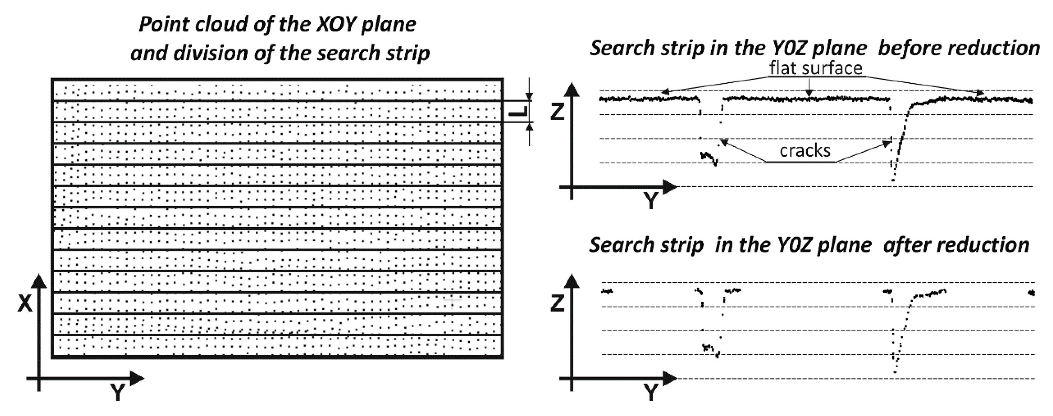
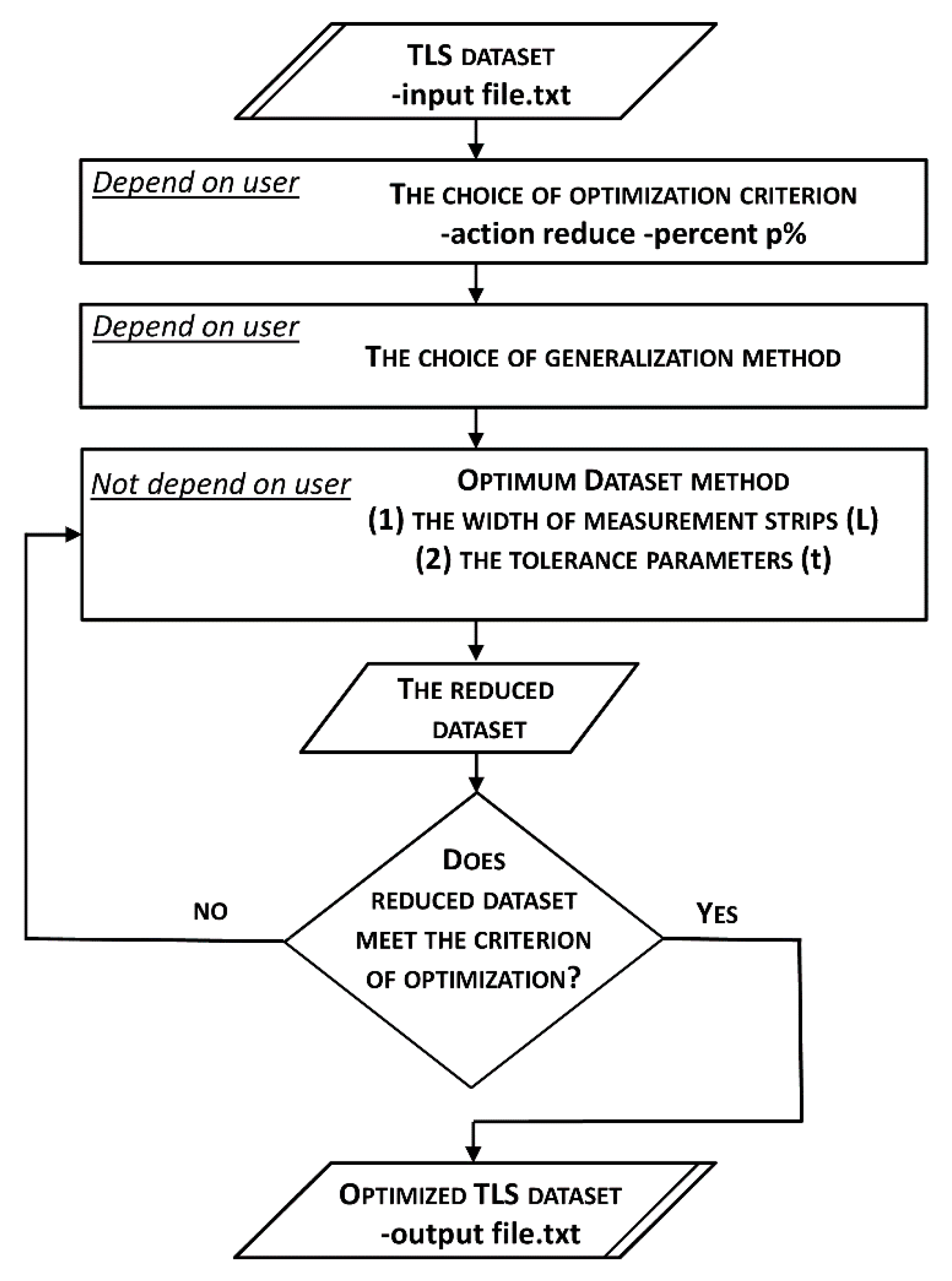
Theoretical Background of OptD Method

The theoretical principles of the algorithm’s operation and the OptD method in various applications have been presented in [30,31]. The OptD method was modified for wall defect detection, and consists of iteratively processed stages. The OptD-single method has been used in this study.

In step 1, the algorithm read the input TLS dataset in *.txt format. Depending on the content of the input file, the user modifies the configuration file. In step 2, the OptD method starts asking to the user to set a proper optimization criterion (f). Such a criterion can specify, for instance, a percentage of the total number of points in the original point cloud, leading to a data reduction of exactly the percentage value specified by (f). This is the most commonly accepted optimization criterion, as the result of optimization is the most characteristic point in the dataset—the higher the degree of reduction, the more visible changes will be on the object. Multiple optimization criteria can also be considered, if needed, in the OptD-multi case [30].

In the next step, step 3, the OptD method starts an automatic and iterative process of data examination and point selection until the desired goal is met. First, the data domain is partitioned in stripes of width L on the horizontal plane (see Figure 1). The width of the strip L is important, as the degree of reduction depends (among others) on this parameter. The initial value L depends on the density of points in the dataset. The input L is taken as the average value of the distance between points. The strips can be horizontal and vertical. It depends on defect characteristics. The width of the measurement strip is automatically calculated and adjusted in subsequent iterations (without the user’s participation). Then, in step 4, the point selection is separately performed on each of such strips by means of the cartographic generalization method [33], whose data reduction rate is strictly related to the current value of the tolerance parameter (t). Since the initial values of L and t automatically set by the OptD method usually do not allow to reach the desired optimization objective, the above process is repeated after automatically resetting the values of such parameters until the obtained results satisfy the chosen criterion. Since this working procedure allows to automatically determine the proper values of L and t, the only human interaction required by the OptD method is the selection of optimization criterion.

The rationale of the point selection principle of the OptD method is based on the idea of preserving more points on the locations where larger variations of the measured variables (e.g., height, intensity of laser beam) occur. Vice versa, fewer points are kept on smooth areas, e.g., where the object shape can be locally well approximated with a planar surface. Consequently, the application of OptD produces point clouds with non-homogeneous densities; the degree of data reduction is highly dependent of the local object shape regularity (i.e., of the information contained in such area of the 3D model). It is also worth noticing that, differently from trivial subsampling methods, OptD checks the usefulness of each point in the model: the tolerance parameter is used to determine whether a point should be preserved or discarded. The reader is referred to [30,31] for a more detailed description of the OptD method.

The result of step 4 depends on the value of the tolerance parameter. The end of the OptD processing process occurs in step 5, when the generalization method will be applied in all measurement strips, and the saved dataset will meet the optimization criterion set in step 2. The width of the measurement strip and the tolerance parameter decide the degree of reduction, therefore these values are changed during iteration until the output dataset meets the optimization criterion.

Figure 2 summarizes the workflow of the OptD method, taking into account all the parameters that affect the reduction results.

In the scheme, the parameters that are dependent and not dependent on the user are visible. In the iterative process, a dataset that meets the optimization criterion is selected. It should be mentioned that with the use of TLS, the one wall or the entire object are measured. To apply the OptD method, each wall must be implemented separately in the local wall coordinate system. It is important that the wall with defects is in the correct coordinate system, so that the correct division into measuring strips occurs.

The use of the OptD method has a positive impact on the following aspects:

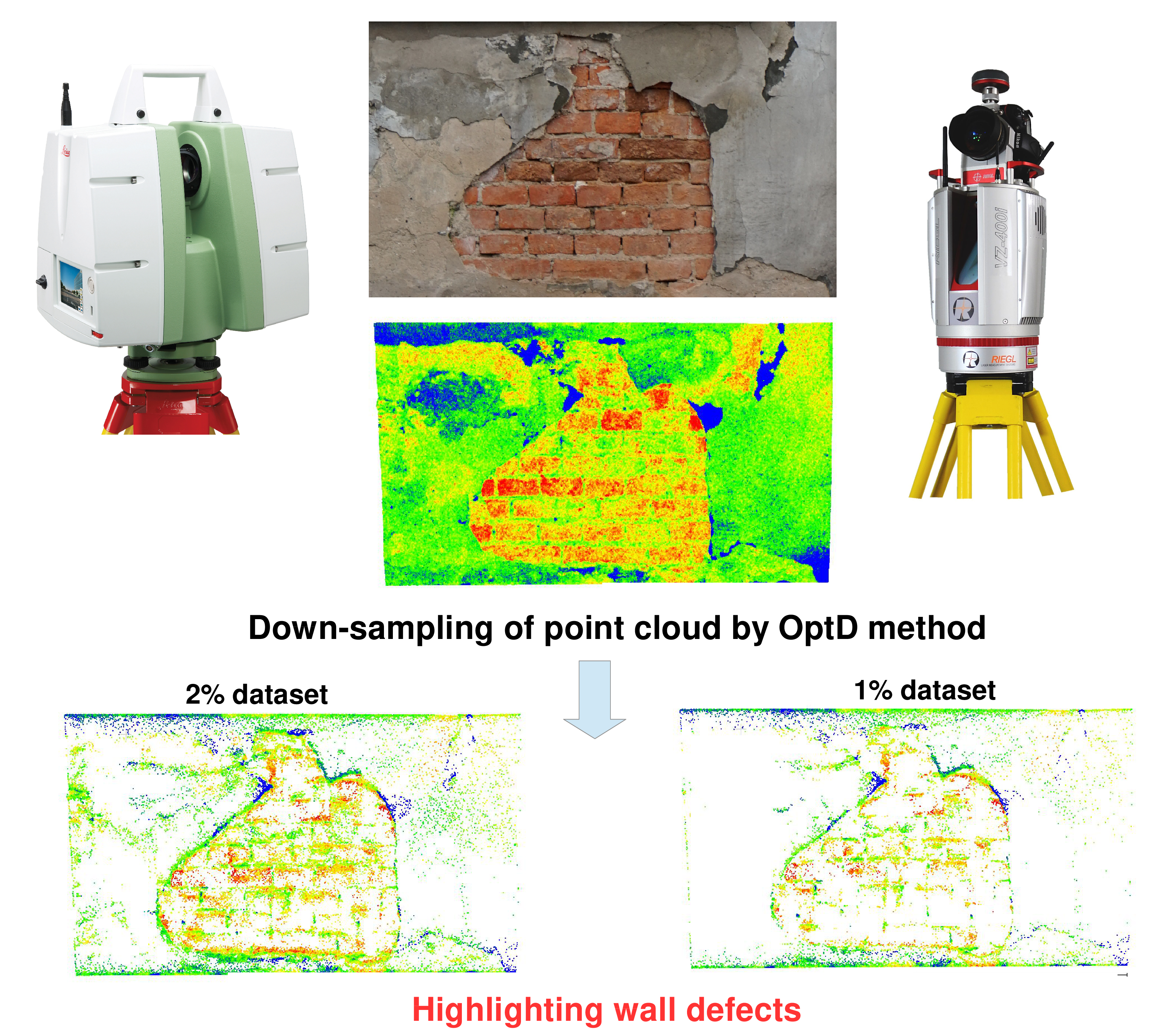
• Geometry visibility. Improvement of visibility and readability of the certain shape details. After applying OptD, it is possible to better distinguish object shapes that might originally be hardly visible because of the presence of a large amount of data [34];
• Processing time. Dataset reduction enables a computationally more efficient execution of the time-consuming analysis of the acquired data [30].

In previous papers using the OptD method, the advantage of the method was the processing speed, especially when DTM is generated based on a reduced point cloud.

In [30], the results showed that with the OptD method, the preparation of the data or DTM construction is less time-consuming. The time required for the implementation of the OptD method can be considered as negligible in the whole process of preparing the data for the DTM construction. In the work, [35] has shown that the approach based on the OptD method is less time- and labour-consuming than the approach based on DTM generalization. It results from the fact that before the DTM is generalized, it must first be built from the original point cloud. If the OptD method is used, the dataset will be quickly reduced and DTM will be generated on the basis of the optimal dataset. During the DTM generalization, the time needed to reduce the dataset was about 1200 s. Meanwhile, for reduction using the OptD method it was up to 20 s. In both approaches, datasets can be reduced by up to 98%.

Furthermore, in the case of MLS data for a dataset consisting of 20 million points, the OptD method lasted for about 72 s (for criterion of optimization equal to 50%) and 121 s (for criterion of optimization equal to 90%) [36].

3. Results

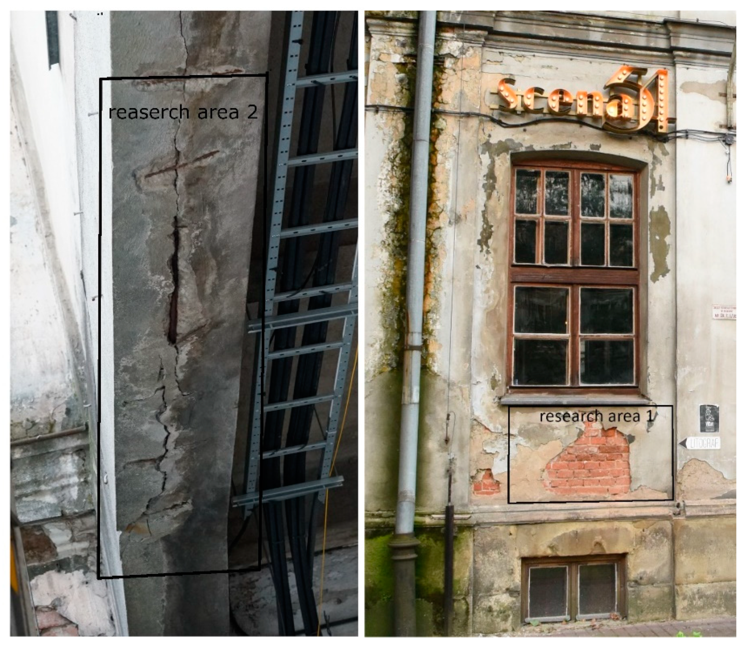
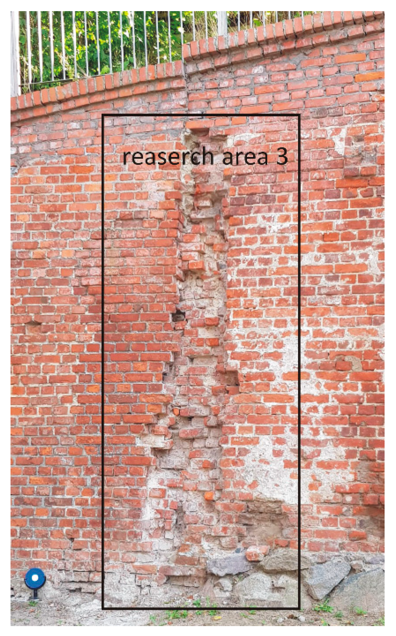
3.1. Objects of Research and Used Equipment

In this work, two different time-of-flight terrestrial laser scanners, Riegl VZ-400i and Leica ScanStation C10, were used.

The Riegl VZ-400i TLS uses a narrow infrared laser beam. Laser pulse repetition is from 100 kHz to 1200 kHz. The maximum measurement range of this TLS is up to 800 meters for a laser pulse repetition rate of 100 kHz. The scanner works with a maximum measurement rate of 500,000 points/s for a laser pulse repetition rate of 1200 kHz. The laser beam divergence is 0.35 mrad. The angle measurement resolution is better than 0.0007°, and the range accuracy at 100 m is 5 mm.

The Leica ScanStation C10 TLS uses a visible green laser beam (wavelength equal to 532 nm). The maximum and minimum measurement ranges are approximately 300 m and 0.1 m, respectively. The Leica ScanStation C10 scanner has scan speed of up to 50,000 points/s. The laser beam width at 50 m is 4.5 mm (full-width-half-maximum). Angular accuracy is 60 μrad, while range and position measurement accuracies at 50 m are 4 mm and 6 mm, respectively.

The first case study considered in this work is an old tobacco factory in Cracow. The building is part of the Dolne Młyny complex, which is under the supervision of the conservator. The interior part of the building has been restored, while the outer part of the building is in poor technical condition. A part of wall with damaged plaster and concrete structural element with cracks (Figure 3) was used to carry out the tests. Measurements were conducted with Riegl VZ-400i TLS at 10 m distance from the wall, setting the laser pulse repetition rate to 1200 kHz. The angular measurement resolution, both horizontal and vertical, was set on the scanner to 0.01 deg.

The second case study was the historic retaining wall strengthening the bluff located in Olsztyn (Figure 4). The TLS survey was conducted with a Leica ScanStation C10 from two stations in order to properly scan the entire deep cavity. The two-point clouds were registered using special targets and merged using the Cyclone software.

The registration results are shown in

Table 1. Point clouds registration report.

ID	ScanWorld	ScanWorld	Weight	Error [m]	Error Vector [m]	Error Horz [m]	Error Vert [m]
1	SW-002	SW-003	1	0.001	(−0.001, 0.000,0.000)	0.001	0.000
2	SW-002	SW-003	1	0.001	(0.000, 0.001,0.000)	0.001	0.000
3	SW-002	SW-003	1	0.000	(0.000, 0.000,0.000)	0.000	0.000
4	SW-002	SW-003	1	0.000	(0.000, 0.000,0.000)	0.000	0.000

.

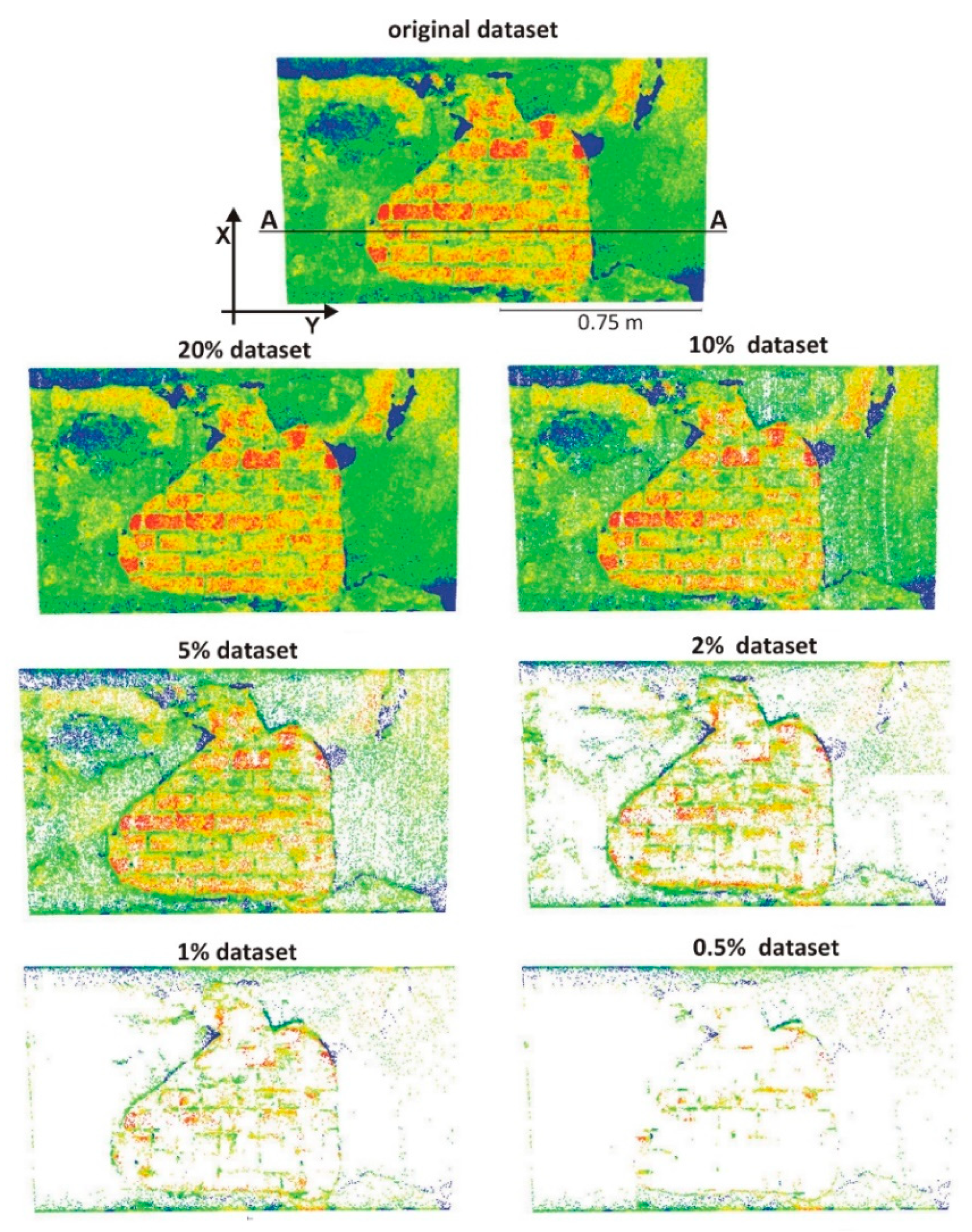
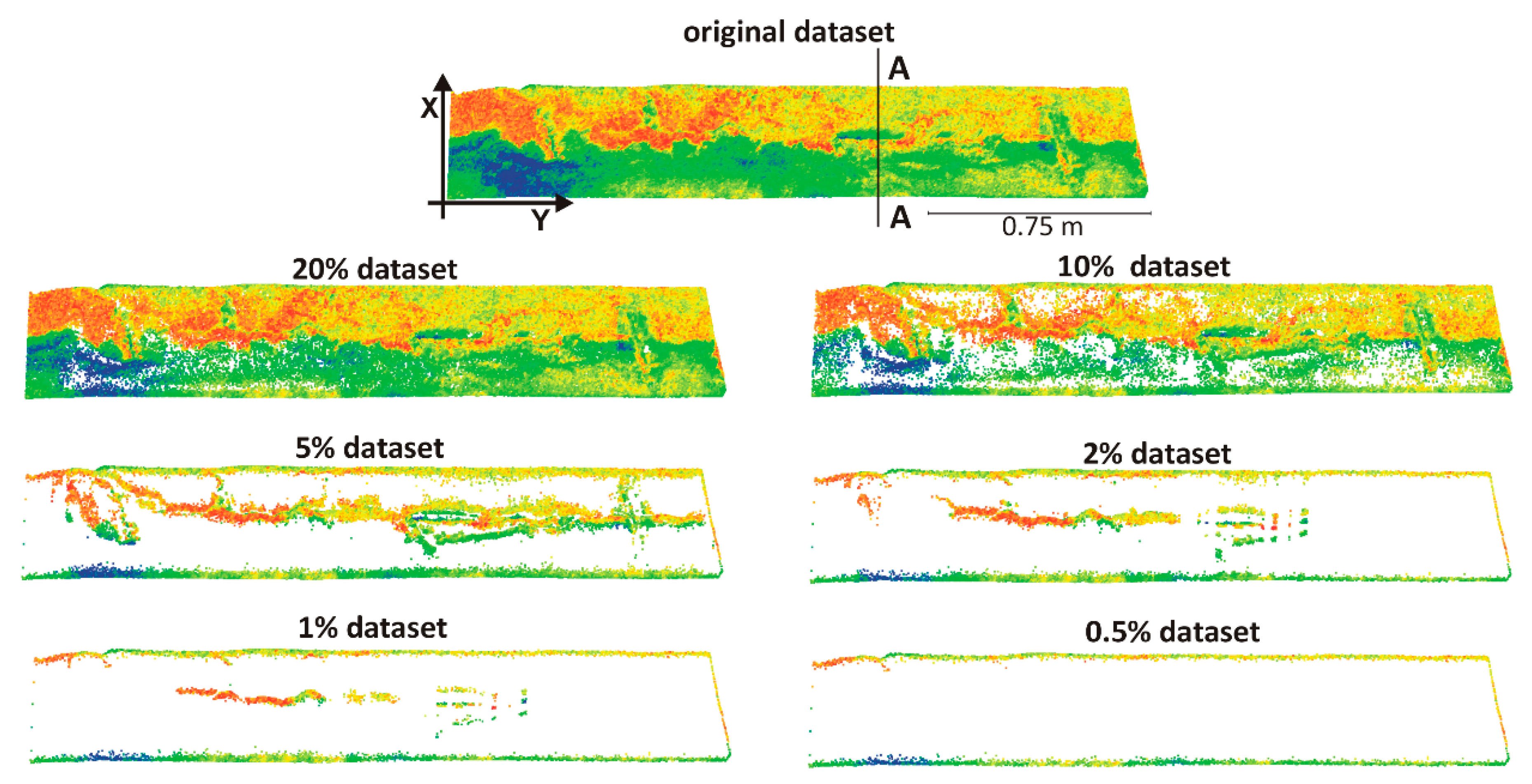
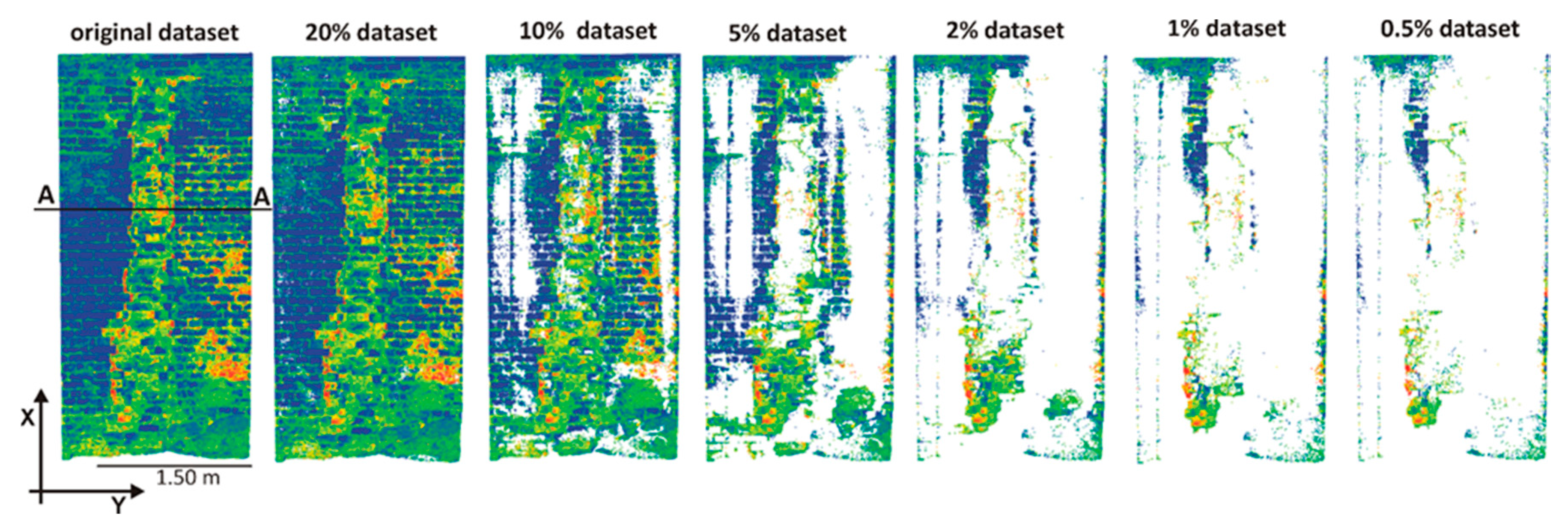
3.2. Data Processing Using the OptD Method

The CloudCompare software was used to visualize the data. Detailed characteristics of the datasets used in this work as case studies are provided in

Table 2. Characteristics of the case study datasets.

Sample	Dimensions [m]	No points
wall with damaged plaster	1.50 ∙ 0.90	2,377,449
concrete element with cracks	2.30 ∙ 0.38	762,480
damaged brick wall	3.92 ∙ 1.85	7,272,966

.

The TLS datasets were processed by means of the OptD method. Authors used their own software to reduce the datasets. The software has been written in the Java programming language (v.9). The percentage of points to be retained after the data reduction was used as the optimization criterion in the OptD. During processing, the Douglas–Peucker generalization method was used. For comparison, the OptD method was run with six different settings, i.e., with the following values of the percentage of points to be retained: 20%, 10%, 5%, 2%, 1% and 0.5%.

Table 3. Parameters adopted by the algorithm.

p%	20%	10%	5%	2%	1%	0.5%
Wall with damaged plaster
L [m]	0.001	0.001	0.001	0.001	0.001	0.001
t [m]	0.002	0.003	0.004	0.009	0.016	0.031
Iterations	9	14	14	13	11	10
Concrete element with the cracks
L [m]	0.001	0.001	0.001	0.001	0.001	0.001
t [m]	0.002	0.003	0.005	0.013	0.022	0.036
Iterations	15	13	13	12	12	10
Damaged retaining brick wall
L [m]	0.005	0.005	0.005	0.005	0.005	0.005
t [m]	0.073	0.215	0.678	0.752	0.821	0.954
Iterations	10	7	6	10	10	11

reports the values of the processing parameters, namely L and t, automatically determined by the OptD to satisfy the optimization requirements.

Table 3 presents L and t for the last iteration. For all test objects, the L value was the same for the last iteration with the adopted optimization criteria: 0.001 m for test area 1 (wall with damaged plaster) and test area 2 (concrete element with the cracks, respectively, and 0.005 m for test area 3 (damaged retaining brick wall). However, the value of t changed depending on the optimization criterion. The most iterations were needed when processing test area 2 with the optimization criterion p = 20%, while the least iterations were for test area 3 with p = 5%. The largest t-value was for test area 3 at p = 0.5%. This is due to the fact that this feature was the most diverse in terms of geometry.

The data reduction results obtained in the test areas 1, 2 and 3 are shown in Figure 5, Figure 6 and Figure 7, respectively.

The main advantage of the OptD method is that it typically ensures a low data reduction rate on areas corresponding to defects (cavities, cracks or other surface discontinuities) and, vice versa, a high reduction rate on smooth/regular areas (without defects). This can clearly be seen by means of visual inspection in the presented examples (Figure 4, Figure 5 and Figure 6). For instance, the number of points in the 2% and 1% datasets in Figure 4 were largely reduced on the flat areas, while leaving many more points on the defects of the wall.

A similar observation can be repeated for the 5%, 2% and 1% datasets in Figure 5 and Figure 6.

It is also notable that in all the considered cases (see Figure 4, Figure 5 and Figure 6), the 0.5% dataset probably does not allow a proper defect detection. This is a direct consequence of the dramatic data reduction and the specific behaviour of the OptD algorithm, which always preserves a significant amount of points on the borders of the considered area.

AA profiles were made for three cases to carefully analyze the obtained results, which are shown in Figure 8, Figure 9 and Figure 10. The profiles show strips of 0.008 m width.

It is worth noticing that points close to sudden profile changes should be preserved by the data reduction method to properly maintain the possibility of defect detection on the wall surface. Positions corresponding to such sudden changes are marked with dashed lines in figures to ease the readability of these figures.

In Figure 8, a dashed line was located in mortar layers. In most cases, the mortar layers have been damaged. By analyzing the individual profiles, it can be concluded that the OptD reduction method left more points in the above-mentioned places than on the flat surfaces, which was expected.

The profiles shown in Figure 9 correspond to a defected area in the concrete element. As shown in this figure (e.g., 2% dataset), the OptD method clearly retains a larger amount of points on areas associated with profile variations, which are more informative for detecting defects.

The profiles shown in Figure 10 correspond to a defected area in the brick wall. For instance, by analyzing these profiles, it can be seen that for a 5% dataset, one can correctly diagnose the defect. Thus, the OptD method also works well in this case.

4. Discussion

Since OptD retains a larger number of points on defected areas, it is quite clear that it allows high data reduction rates while still preserving the possibility of detecting cavities and cracks. In spite of this, the selection of a very high down-sampling rate may cause the loss of useful information about object defects.

A more in-depth analysis of three samples taken from the considered datasets were carried out in order to better investigate this aspect (Figure 11). Each sample has a flat and homogeneous area (FHA) and defect area (DA). The quantitative comparisons between the original and reduced point cloud for FHA and DA are presented in

Table 4. Results of down-sampling of point cloud for three samples.

	Flat and Homogeneous Area (FHA)		Defect Area (DA)			$\frac{\mathbf{DA}\mathbf{\%}}{\mathbf{FHA}\mathbf{\%}}$
	Number of Points	Percentage	Number of Points	Percentage	Density Points/0.01m2
Wall with damaged plaster
original dataset	181,062	100.000%	204,813	100.000%	17,226	1
20% dataset	24,664	13.622%	42,651	20.824%	3587	2
10% dataset	16,370	9.041%	29,638	14.471%	2493	2
5% dataset	4881	2.696%	20,130	9.828%	1693	4
2% dataset	305	0.168%	8441	4.121%	710	24
1% dataset	49	0.027%	3257	1.590%	274	59
0.5% dataset	5	0.003%	993	0.485%	84	176
Concrete element with the cracks
original dataset	45,351	100.000%	20,912	100.000%	12,560	1
20% dataset	3,544	7.815%	6835	32.685%	4105	4
10% dataset	1,464	3.228%	5572	26.645%	3347	8
5% dataset	12	0.026%	3456	16.526%	2076	625
2% dataset	11	0.024%	1992	9.526%	1196	393
1% dataset	1	0.002%	952	4.552%	572	2065
0.5% dataset	0	0.000%	0	0.000%	0	–
Damaged retaining brick wall
original dataset	466,071	100.000%	663,249	100.000%	9116	1
20% dataset	52,965	11.364%	122,862	18.524%	1689	2
10% dataset	22,841	4.901%	62,539	9.429%	860	2
5% dataset	52	0.011%	29,789	4.491%	409	403
2% dataset	15	0.003%	1860	0.280%	26	87
1% dataset	10	0.002%	497	0.075%	7	35
0.5% dataset	4	0.001%	317	0.048%	4	56

. As a result of a visual assessment, it was found that considering the 2% dataset is sufficient to execute a proper diagnosis of both the wall with damaged plaster and the concrete element with cracks. Differently, the 5% dataset shall be used in the case of damaged retaining brick wall. Figure 11 reports the percentage of points kept in the FHA and DA in all considered cases.

Figure 12 presents a spatial visualization for test area 3, as this object was the most diverse in terms of geometry and had the largest defects.

Figure 12 presents the distribution of points that obstruct a homogeneous area and defect area. The figure was prepared based on the sets after the optimization criterion of 5% (similar to Figure 11) and the level above, i.e., 10%. OptD processing results in a different degree of reduction in different areas of the object. On places that are not very varied, few points remained (red colour in Figure 12), and on complex surfaces there were more points (blue colour in Figure 12). Thanks to this property of the OptD method, we can find object defects while reducing the size of the dataset.

Table 4 and Figure 13 experimentally prove that the data reduction on the flat and homogeneous areas is greater than on the defect area, which was expected. Nevertheless, the reduction degree in these areas differs for different datasets.

For instance, in the first case study, in the 5% dataset 2.696% of the original amount of points were retained in the FHA area, while 9.828% points were retained in the DA area, leading to approximately four times more points kept in the DA with respect to FHA (DA%/FHA% ≈ 4). Differently, in the 2% dataset case, only 0.168% points are retained on the FHA area and 4.121% points in the DA area, leading to a 24-times ratio between the two of them. Similar considerations can also be repeated in the other cases reported in Table 4.

To conclude, according to the analysis conducted in this work, the OptD method can be effectively used for point cloud down-sampling in the context of identifying building defects. The shrunk dataset obtained from the OptD method can be more easily visually analysed or processed further using algorithms for automatic point cloud classification.

Analysing the graphs presented in Figure 13, it can be seen that the largest discrepancies in the retained points between the homogeneous area and defect area occur for concrete element (test area 2). This means that for this case, more unnecessary points have been removed (in areas with little variation) compared to the points showing the defects.

5. Conclusions

The paper presents the application of the OptD method for the optimized size reduction of point clouds in the diagnosis and monitoring of historical buildings. Results reported in this paper show that, thanks to its careful optimized point selection, the use of OptD allows to obtain a significantly smaller dataset while also highlighting defects and discontinuities in the wall with damaged plaster in the concrete element, as well as the brick wall.

Based on the results obtained in the considered case studies, the following conclusions can be drawn:

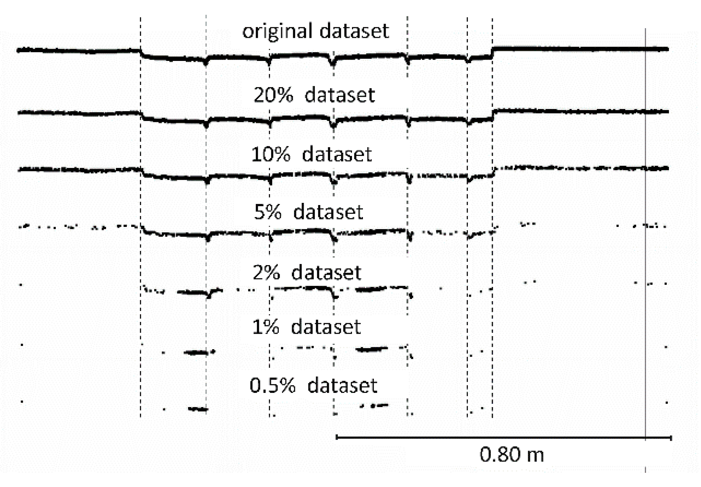
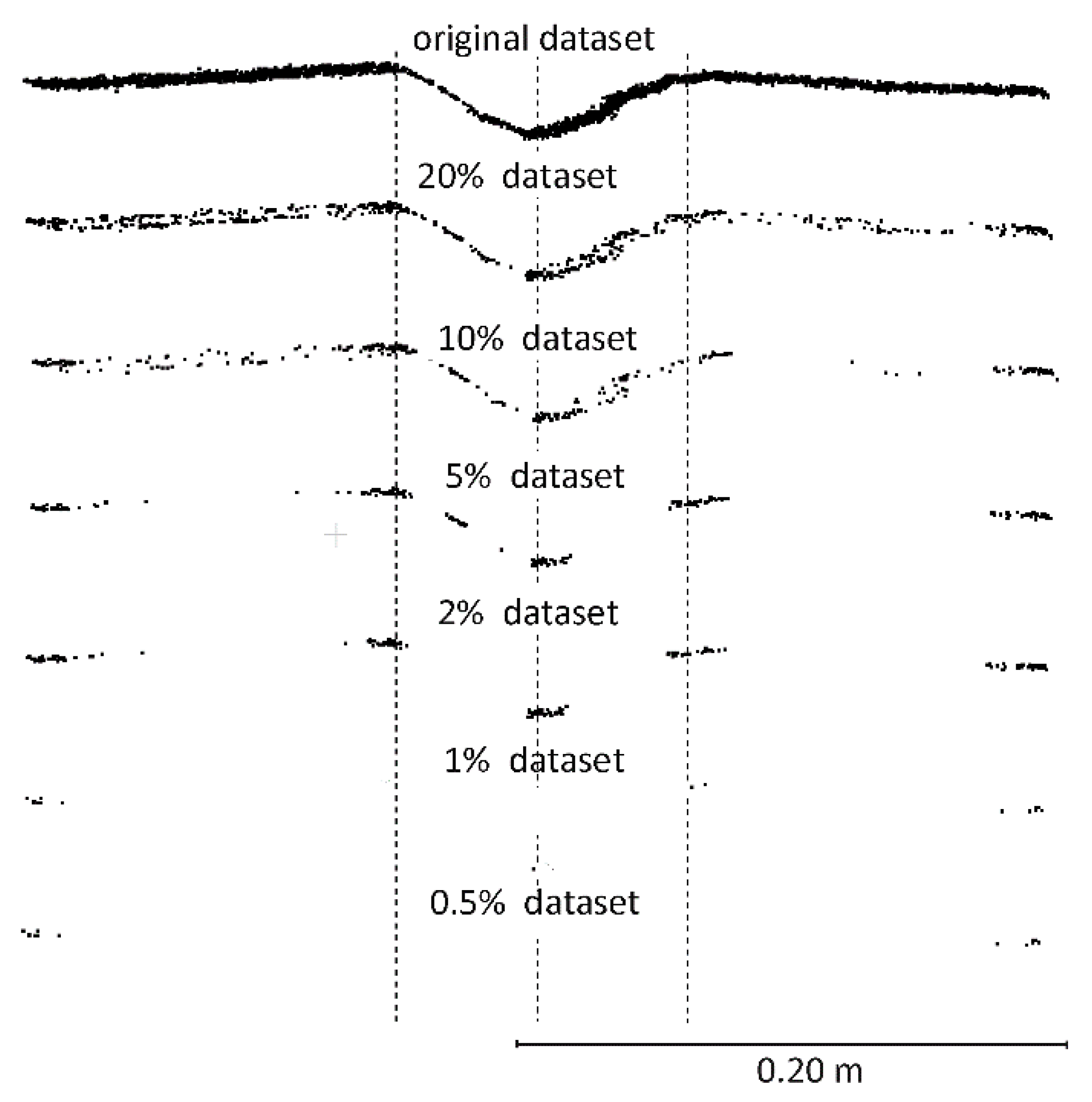
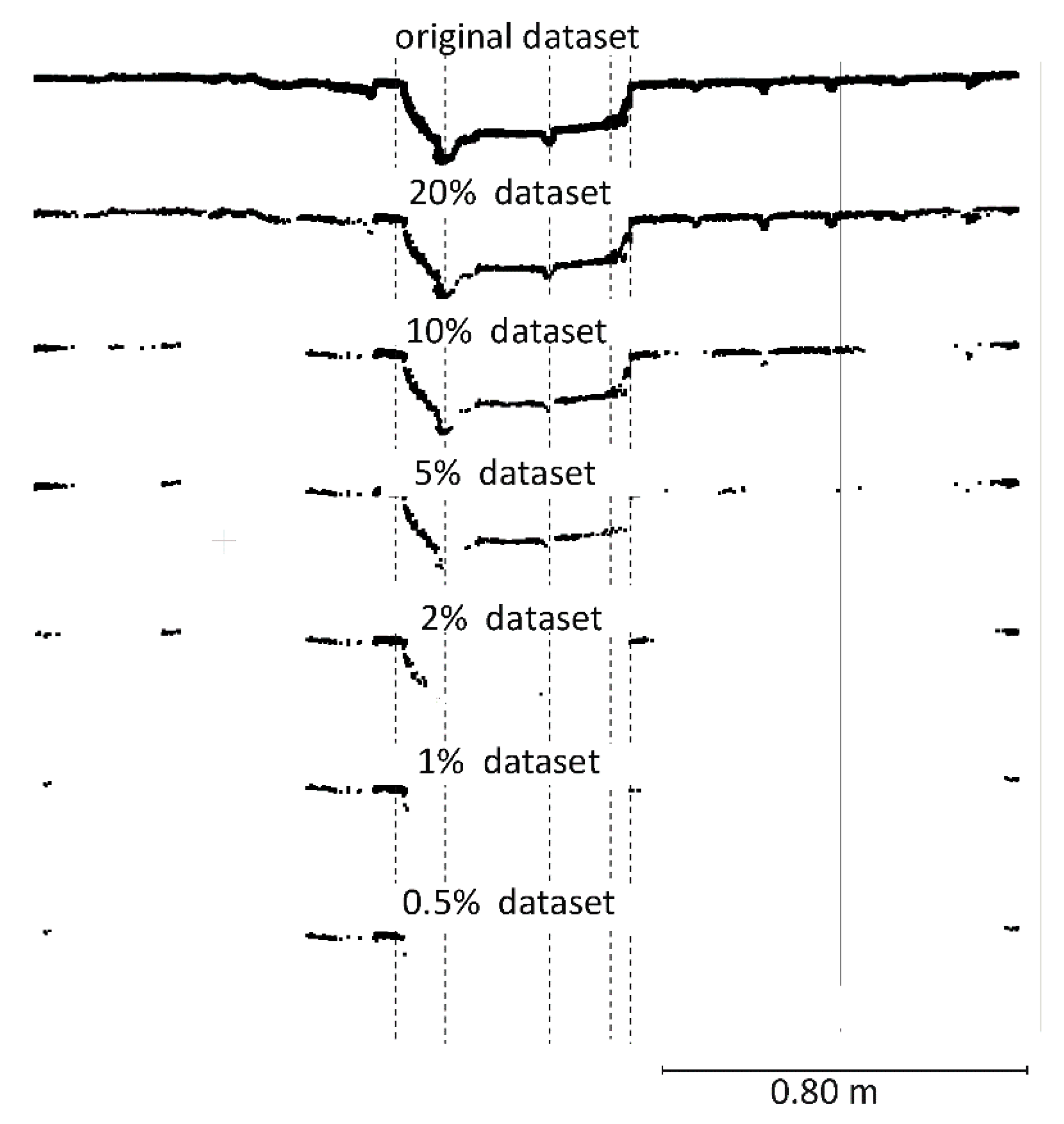
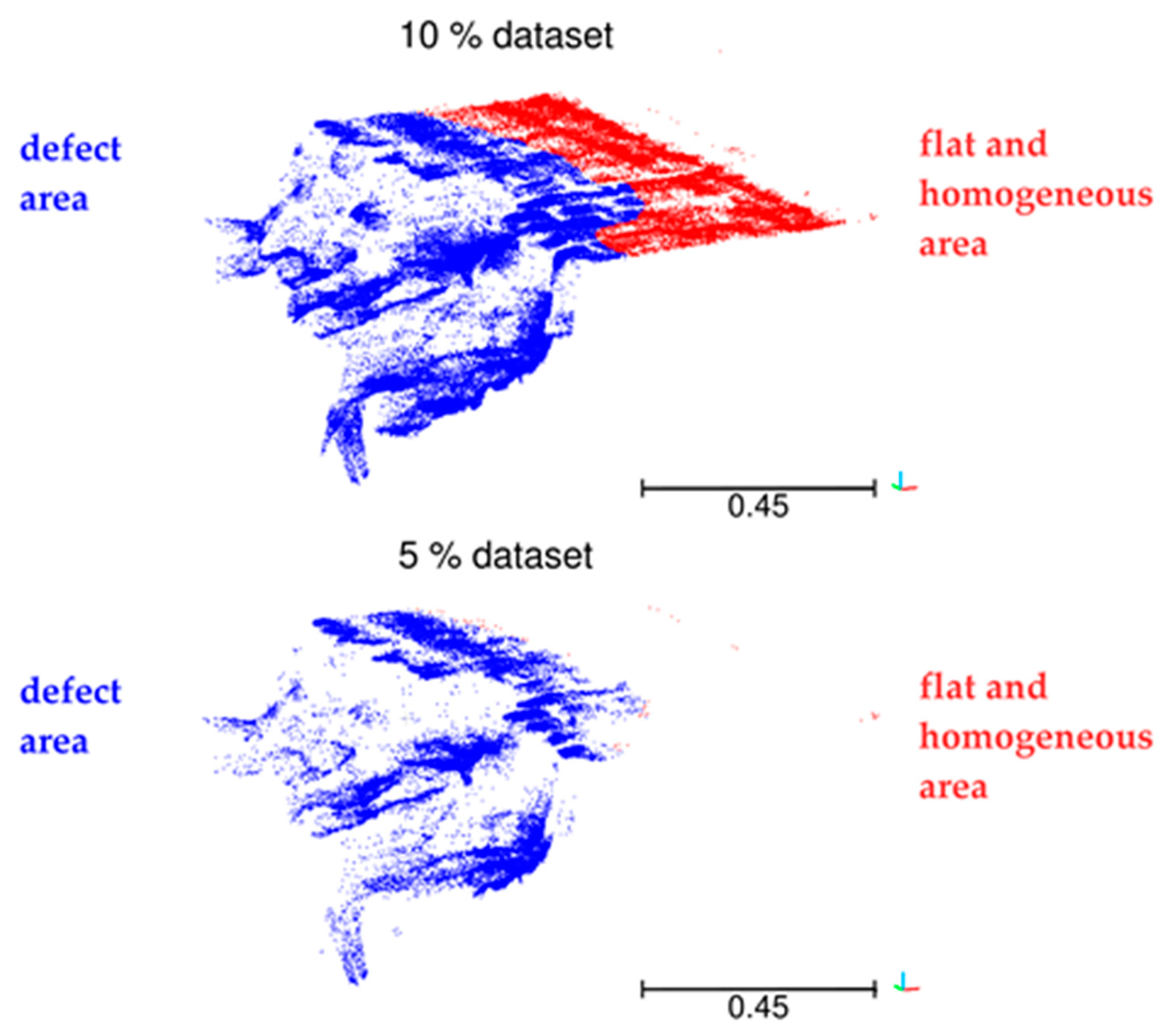
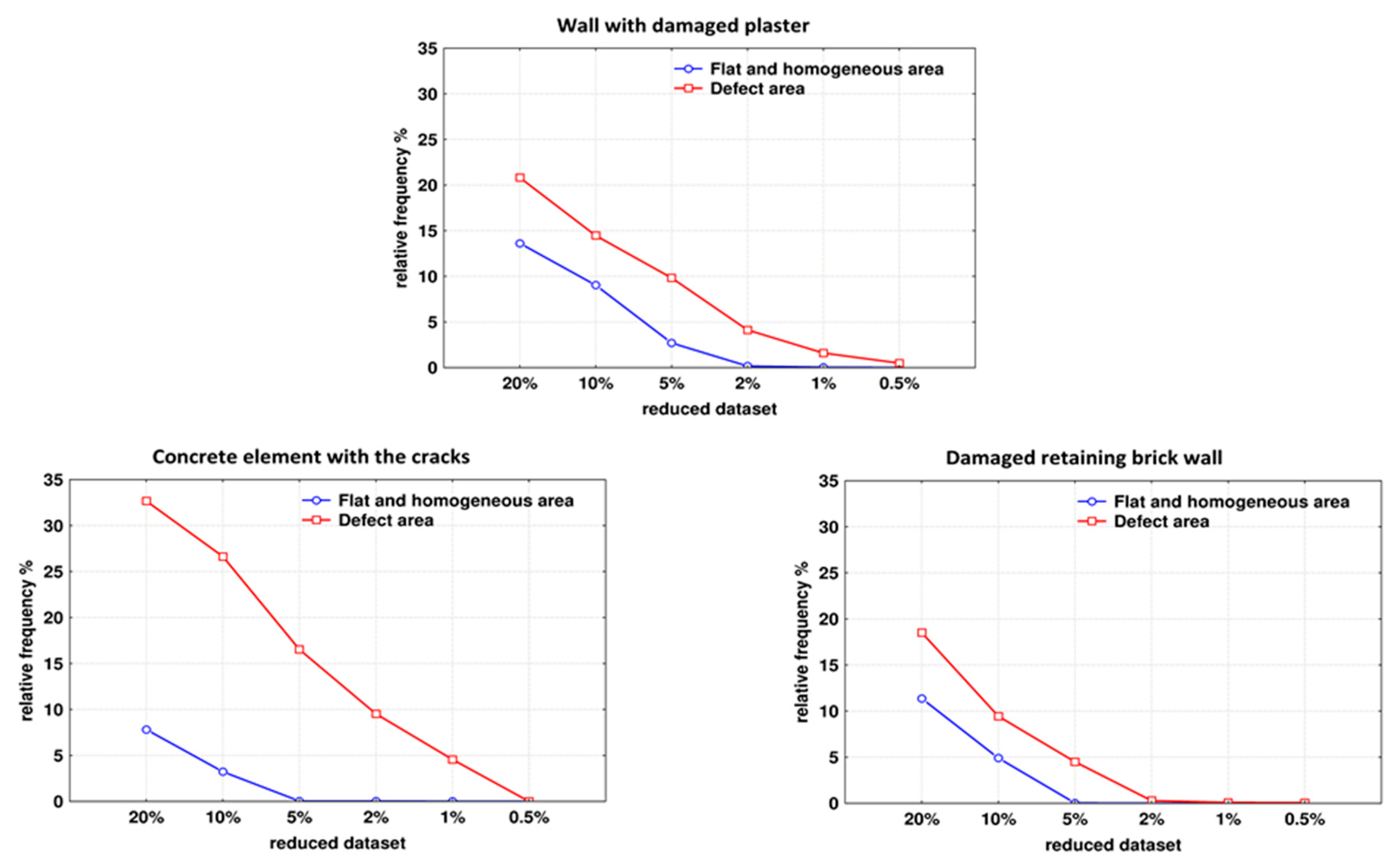
• The reduced dataset obtained with OptD has a significantly lower point density on regular areas (wall without defects) than on defects (cavities and cracks).
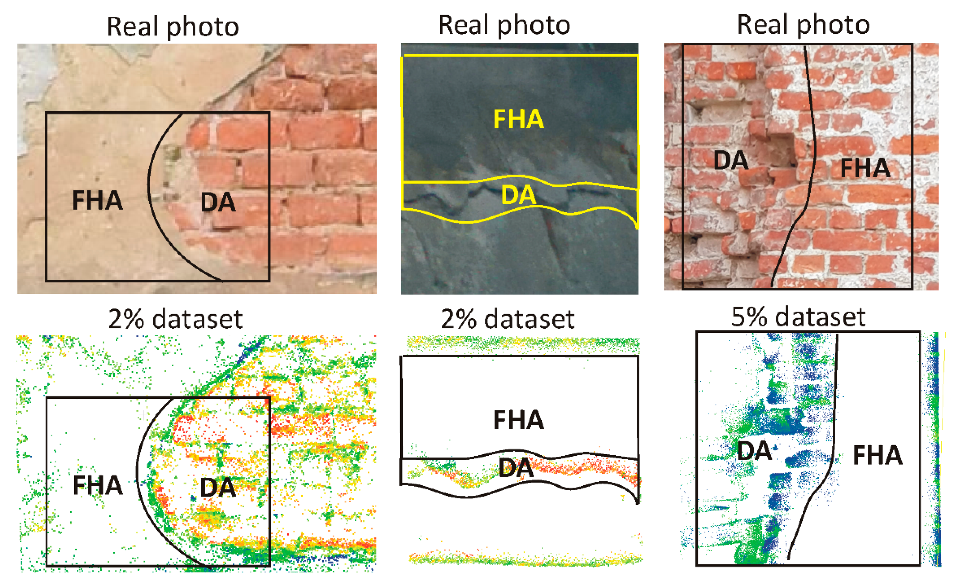
• Obtained results show that OptD can be effectively used for optimizing cloud points for diagnostic measurements buildings and other structures.
• The results of this work indicate the possibility of using OptD as a tool for easing the detection of defects in buildings and structures. Our future work will be dedicated to the investigation of this aspect.
• The main disadvantage of the OptD method is that it may retain a large number of points at the border of the region of interest.
• Authors have been working to implement the OptD method in point cloud data processing software.

References

1. Lague, D.; Brodu, N.; Leroux, J. Accurate 3D comparison of complex topography with terrestrial laser scanner: Application to the Rangitikei canyon (N-Z). ISPRS J. Photogramm. Remote Sens. 2013, 82, 10–26. [Google Scholar] [CrossRef] [Green Version]
2. Reshetyuk, Y.; Mårtensson, S.G. Terrestrial laser scanning for detection of landfill gas: A pilot study. J. Appl. Geod. 2014, 8, 87–96. [Google Scholar] [CrossRef]
3. Ossowski, R.; Przyborski, M.; Tysiac, P. Stability Assessment of Coastal Cliffs Incorporating Laser Scanning Technology and a Numerical Analysis. Remote Sens. 2019, 11, 1951. [Google Scholar] [CrossRef] [Green Version]
4. Kasperski, J.; Delacourt, C.; Allemand, P.; Potherat, P.; Jaud, M.; Varrel, E. Application of a Terrestrial Laser Scanner (TLS) to the study of the Séchilienne landslide (Isère, France). Remote Sens. 2010, 2, 2785–2802. [Google Scholar] [CrossRef] [Green Version]
5. Suchocki, C. Application of terrestrial laser scanner in cliff shores monitoring. Rocz. Ochr. Sr. 2009, 11, 715–725. [Google Scholar]
6. Nowak, R.; Orłowicz, R.; Rutkowski, R. Use of TLS (LiDAR) for building diagnostics with the example of a historic building in Karlino. Buildings 2020, 10, 24. [Google Scholar] [CrossRef] [Green Version]
7. Kermarrec, G.; Kargoll, B.; Alkhatib, H. Deformation analysis using B-spline surface with correlated terrestrial laser scanner observations-a bridge under load. Remote Sens. 2020, 12, 829. [Google Scholar] [CrossRef] [Green Version]
8. Suchocki, C.; Katzer, J. TLS technology in brick walls inspection. In Proceedings of the 2018 Baltic Geodetic Congress (BGC Geomatics), Olsztyn, Poland, 21–23 June 2018; pp. 359–363. [Google Scholar]
9. Suchocki, C.; Damięcka, M.; Jagoda, M. Determination of the building wall deviations from the vertical plane. In Proceedings of the 7th International Conference on Environmental Engineering, ICEE 2008—Conference Proceedings, Vilnius, Lithuania, 22–23 May 2008; pp. 1488–1492. [Google Scholar]
10. Pu, S.; Rutzinger, M.; Vosselman, G.; Oude Elberink, S. Recognizing basic structures from mobile laser scanning data for road inventory studies. ISPRS J. Photogramm. Remote Sens. 2011, 66, S28–S39. [Google Scholar] [CrossRef]
11. Guan, H.; Li, J.; Yu, Y.; Wang, C.; Chapman, M.; Yang, B. Using mobile laser scanning data for automated extraction of road markings. ISPRS J. Photogramm. Remote Sens. 2014, 87, 93–107. [Google Scholar] [CrossRef]
12. Chmelina, K.; Jansa, J.; Hesina, G.; Traxler, C. A 3-d laser scanning system and scan data processing method for themonitoring of tunnel deformations. J. Appl. Geod. 2012, 6, 177–185. [Google Scholar] [CrossRef]
13. Tan, K.; Cheng, X.; Ju, Q.; Wu, S. Correction of Mobile TLS Intensity Data for Water Leakage Spots Detection in Metro Tunnels. IEEE Geosci. Remote Sens. Lett. 2016, 13, 1711–1715. [Google Scholar] [CrossRef]
14. Yastikli, N. Documentation of cultural heritage using digital photogrammetry and laser scanning. J. Cult. Herit. 2007, 8, 423–427. [Google Scholar] [CrossRef]
15. Grilli, E.; Remondino, F. Classification of 3D digital heritage. Remote Sens. 2019, 11, 847. [Google Scholar] [CrossRef] [Green Version]
16. Armesto-González, J.; Riveiro-Rodríguez, B.; González-Aguilera, D.; Rivas-Brea, M.T. Terrestrial laser scanning intensity data applied to damage detection for historical buildings. J. Archaeol. Sci. 2010, 37, 3037–3047. [Google Scholar] [CrossRef]
17. Suchocki, C.; Jagoda, M.; Obuchovski, R.; Šlikas, D.; Sužiedelytė-Visockienė, J. The properties of terrestrial laser system intensity in measurements of technical conditions of architectural structures. Metrol. Meas. Syst. 2018, 25, 779–792. [Google Scholar] [CrossRef]
18. Suchocki, C.; Katzer, J.; Rapiński, J. Terrestrial Laser Scanner as a Tool for Assessment of Saturation and Moisture Movement in Building Materials. Period. Polytech. Civ. Eng. 2018, 62, 694–699. [Google Scholar] [CrossRef] [Green Version]
19. Suchocki, C.; Katzer, J. Terrestrial laser scanning harnessed for moisture detection in building materials—Problems and limitations. Autom. Constr. 2018, 94, 127–134. [Google Scholar] [CrossRef]
20. Li, Q.; Cheng, X. Damage detection for historical architectures based on tls. In Proceedings of the International Archives of the Photogrammetry, Remote Sensing and Spatial Information Sciences, Beijing, China, 3–11 July 2018; Volune XLII, pp. 7–10. [Google Scholar]
21. Peppe, P.J.; De Donno, G.; Marsella, M.; Orlando, L.; Renzi, B.; Salviani, S.; Santarelli, M.L.; Scifoni, S.; Sonnessa, A.; Verri, F.; et al. High-resolution geomatic and geophysical techniques integrated with chemical analyses for the characterization of a Roman wall. J. Cult. Herit. 2016, 17, 141–150. [Google Scholar] [CrossRef]
22. Nowak, R.; Orłowicz, R. Testing of Chosen Masonry Arched Lintels. Int. J. Archit. Herit. 2020. [Google Scholar] [CrossRef]
23. Peng, J.; Kim, C.S.; Kuo, C.C.J. Technologies for 3D mesh compression: A survey. J. Vis. Commun. Image Represent. 2005, 16, 688–733. [Google Scholar] [CrossRef]
24. Maglo, A.; Lavoue, G.; Dupont, F.; Hudelot, C. 3D Mesh Compression: Survey, Comparisons, and Emerging Trends. ACM Comput. Surv. 2015, 47, 1–44. [Google Scholar] [CrossRef]
25. Du, X.; Zhuo, Y. A point cloud data reduction method based on curvature. In Proceedings of the 2009 IEEE 10th International Conference on Computer-Aided Industrial Design & Conceptual Design—CAID CD’2009, Wenzhou, China, 26–29 November 2009; pp. 914–918. [Google Scholar] [CrossRef]
26. Mancini, F.; Castagnetti, C.; Rossi, P.; Dubbini, M.; Fazio, N.L.; Perrotti, M.; Lollino, P. An integrated procedure to assess the stability of coastal rocky cliffs: From UAV close-range photogrammetry to geomechanical finite element modeling. Remote Sens. 2017, 9, 1235. [Google Scholar] [CrossRef] [Green Version]
27. Lin, Y.-J.; Benziger, R.R.; Habib, A. Planar-Based Adaptive Down-Sampling of Point Clouds. Photogramm. Eng. Remote Sens. 2016, 82, 955–966. [Google Scholar] [CrossRef]
28. Katzer, J.; Kobaka, J. Combined non-destructive testing approach to waste fine aggregate cement composites. Sci. Eng. Compos. Mater. 2009, 16, 277–284. [Google Scholar] [CrossRef]
29. Saint-Pierre, F.; Philibert, A.; Giroux, B.; Rivard, P. Concrete Quality Designation based on Ultrasonic Pulse Velocity. Constr. Build. Mater. 2016, 125, 1022–1027. [Google Scholar] [CrossRef]
30. Błaszczak-Bąk, W.; Sobieraj-Żłobińska, A.; Kowalik, M. The OptD-multi method in LiDAR processing. Meas. Sci. Technol. 2017, 28, 7500–7509. [Google Scholar] [CrossRef]
31. Błaszczak-Bąk, W. New optimum dataset method in LiDAR processing. Acta Geodyn. Geomater. 2016, 13, 381–388. [Google Scholar] [CrossRef] [Green Version]
32. Bauer-Marschallinger, B.; Sabel, D.; Wagner, W. Optimisation of global grids for high-resolution remote sensing data. Comput. Geosci. 2014, 72, 84–93. [Google Scholar] [CrossRef]
33. Douglas, D.H.; Peucker, T.K. Algorithms for the reduction of the number of points required to represent a digitized line or its caricature. Can. Cartogr. 1973, 10, 112–122. [Google Scholar] [CrossRef] [Green Version]
34. Błaszczak-Bąk, W.; Sobieraj-Złobińska, A.; Wieczorek, B. The Optimum Dataset method—Examples of the application. In Proceedings of the E3S Web of Conferences, Wrocław, Poland, 5 January 2018; Volume 26, pp. 1–6. [Google Scholar]
35. Błaszczak-Bąk, W.; Poniewiera, M.; Sobieraj-Żłobińska, A.; Kowalik, M. Reduction of measurement data before Digital Terrain Model generation vs. DTM generalisation. Surv. Rev. 2019, 51, 422–430. [Google Scholar] [CrossRef]
36. Błaszczak-Bąk, W.; Koppanyi, Z.; Toth, C. Reduction Method for Mobile Laser Scanning Data. ISPRS Int. J. Geo-Inf. 2018, 7, 285. [Google Scholar] [CrossRef] [Green Version]
Figure 1. Point cloud reduction in the search strip using the OptD method (step 3 and step 4).
Remotesensing 12 01806 g001
Figure 2. OptD workflow.
Remotesensing 12 01806 g002
Figure 3. The research objects (1-wall with damaged plaster on the left, 2-concrete element with the cracks on the right).
Remotesensing 12 01806 g003
Figure 4. The research object 3, a damaged retaining brick wall.
Remotesensing 12 01806 g004
Figure 5. Results of processing based on OptD-single on test area 1.
Remotesensing 12 01806 g005
Figure 6. Results of processing based on OptD-single method for test area 2.
Remotesensing 12 01806 g006
Figure 7. Results of processing based on OptD-single method for test area 3.
Remotesensing 12 01806 g007
Figure 8. Profiles for test area 1.
Remotesensing 12 01806 g008
Figure 9. Profiles for test area 2.
Remotesensing 12 01806 g009
Figure 10. Profiles for test area 3.
Remotesensing 12 01806 g010
Figure 11. Tested areas for three samples.
Remotesensing 12 01806 g011
Figure 12. Tested area 3 for brick wall samples.
Remotesensing 12 01806 g012
Figure 13. Down-sampling of point cloud on the flat and homogeneous area, and defect area using the OptD method.
Remotesensing 12 01806 g013