Experimental Evidence of Swell Signatures in Airborne L5/E5a GNSS-Reflectometry

Abstract

As compared to GPS L1C/A signals, L5/E5a Global Navigation Satellite System-Reflectometry (GNSS-R) improves the spatial resolution due to the narrower auto-correlation function. Furthermore, the larger transmitted power (+3 dB), and correlation gain (+10 dB) allow the reception of weaker reflected signals. If directive antennas are used, very short incoherent integration times are enough to achieve good signal-to-noise ratios, allowing the reception of multiple specular reflection points without the blurring induced by long incoherent integration times. This study presents for the first time experimental evidence of the wind and swell waves signatures in the GNSS-R waveforms, and it performs a statistical analysis, a time-domain analysis, and a frequency-domain analysis for a unique data set of waveforms collected by the UPC MIR instrument during a series of flights over the Bass Strait, Australia.

1. Introduction

The Microwave Interferometric Reflectometer (MIR) is an airborne multi-constellation, dual-beam, and dual-band (L1/E1 and L5/E5a), conventional and interferometric GNSS-R [1] instrument (Figure 1). It has two very directive antenna arrays to pick the direct and reflected GNSS signals [2,3]. MIR was conceived for real-time processing, but raw data is also stored at 32.768 MS/s at 1 bit I/Q for offline processing. One of its maiden flights was over the Bass Strait that separates Australia and Tasmania. The large antenna directivity (18.1 dB for the down-looking array @ L5/E5a) allows a clean detection of the reflected signal even with short incoherent integration times (40–300 ms). In these conditions, the peak of the reflected signal is not blurred, and re-tracking is not required. This has allowed that multiple peaks systematically appear in the Delay-Doppler Maps (DDM) and waveforms (WF), provided they occur within the antenna footprint. As it is presented in this study, these multiple peaks are related to sea wave information, produced by multiple reflections on consecutive waves, producing a forward Bragg scattering in consecutive wave crests.

Wind-driven and swell period or wavelengths have both been measured using other remote sensing techniques such as High Frequency (HF) radar [4], where the HF signal is back Bragg scattered over multiple swell crests, and the signal retrieved contains a modulation in frequency based on the scattered signal. Swell retrieval has been also conducted using microwaves signals, as the approach using a Doppler radar at S-Band [5], where both wind sea and swell components can be measured through spectral analysis. Moreover, Synthetic Aperture Radar (SAR) instruments have also retrieved swell parameters from space based on spectral estimation, as in Sentinel-1 [6]. As seen, most of those measurements are based on a back Bragg scattering mechanism in consecutive wave crests (Chapter 10 of [7]).

The same physical principle is presented in this study, but using GNSS-R signals in a forward scattering configuration. As stated in [8], swell components can only be seen using large bandwidth signals with narrow auto-correlation functions. Examples are given for resolutions up to 30 m. However, this is not the case for current GNSS-R instruments, which are nearly all designed to work with GPS L1 C/A signals, with 300 m spatial resolution (width of the auto-correlation function). However, the use of a higher spatial resolution signal, such as the GNSS L5 (with a spatial resolution of 30 m), opens the possibility to measure the swell spectra, as the spatial resolution provided by these signals is comparable to the swell wavelength, as will be covered in the next section.

2. Data set Description and Validation Data

On 6th June 2018 MIR flew over the Bass Strait, Australia, installed on an airplane flying at ∼1500 m height, and at speed of 74 m/s. During the post-processing of the waveforms generated by MIR (as shown in [9]), it has been found that most L5/E5 waveforms have second peak. In order to illustrate it, two different tracks have been selected, as shown in Figure 2 and Figure 3. Each track has two beams directly pointing to a GNSS satellite reflection, as detailed in

Table 1. Track, beam, PRN, and mean incidence angle of the measurement.

Track ID	Beam ID	Constellation and PRN	Incidence Angle (°)
1	1	GPS #1	40
1	2	GPS #32	52
2	1	Galileo #3	20
2	2	GPS #3	42

, which summarizes the metadata information of the reflection, including the satellite PRN, constellation, and the reflection incidence angle to each of the tracks shown in Figure 3. Incidence angle is defined as the angle between transmitter-to-specular point ray and the zenith vector perpendicular to the reflection surface, which is assumed flat for the sake of simplicity.

The data acquired by MIR is sampled at 32.768 MS/s, packetized, and time-tagged every 300 ms. In order to ease the data processing scheme, a single 300 ms packet is used for a single waveform, but a much shorter incoherent integration time of 40 ms is used to avoid blurring of the waveform due to the plane movement. Taking into account the plane speed (74 m/s), and the incoherent integration time (40 ms), the blurring corresponds to an integration over ∼3 m. In addition, the generation rate of the waveform (i.e., the final observable) is at 3.33 Hz, or one every 300 ms, hence each waveform is separated ∼22 m.

In order to understand the origin of all the secondary peaks observed in the waveforms (see Section 3), the sea state conditions during the flight are studied. As there is a lack of in situ buoy information in the area, the ICON model [10] wind wave period [s], swell wave period (s), and wind speed over the sea [m/s] are shown in Figure 2. The waves shown in Figure 2a have a period of $T_{wind}\approx 5$ s, and they are moving with a look angle with respect to the plane trajectory of ∼50°. The swell waves (Figure 2b) have a period of $T_{swell}\approx 9$ s, and the look angle with respect to the plane trajectory is ∼120°. Both wind-driven and swell wave period are related to the wave speed, and therefore to the waves wavelength (${\mathsf{\Lambda }}_{waves}$) [11] (i.e., distance between the crests of the wave) by means of Equation (1).

$$\begin{array}{l}\hfill C_{waves}=1.56·T_{waves},\\ \hfill {\mathsf{\Lambda }}_{waves}=C_{waves}·T_{waves},\end{array}$$

(1)

where $C_{waves}$ is the sea wave celerity (or speed (m/s)), and $T_{waves}$ is either the swell period $T_{swell}$ or the wind-driven period $T_{wind}$ as defined in the previous section. In deep water conditions, the relationship between them is the above closed formula.

Note that the nomenclature used in this study is $X_{waves}$ (X stands for any parameter as C, T, or $\mathsf{\Lambda }$) for any measurement that is not directly related to either wind-driven or swell waves, and $X_{wind}$ or $X_{swell}$ for any measurement directly related to the wind or the swell respectively, retrieved from the ICON model.

In the case under study, the wavelengths of the wind and swell waves are between 39 m and 126 m. Note that, the aggregation of the different waves may cause a different set of wavelengths or periods right with a minimum wavelength of 39 m and a maximum wavelength of 126 m. The following sections show a complete analysis of this second peak and its relations to the sea state conditions. As stated in [12,13], wind-driven and swell waves are combined forming different waves with different periods and heights. The wind and swell components (or even multiple swell components) can be separated by means of spectral analysis [14].

3. Sea Wavelength Retrieval from Waveforms

As in most GNSS scenarios, and due to the sea surface roughness, the combination of both swell waves and wind-driven waves cause multiple reflections, which are then captured by the down-looking antenna of the GNSS-R instrument. Despite that, and as seen in other works [9,16], the reflection over the sea surface presents a notable coherent component, which depends on the geometry of the reflection and the wind speed. Most of the waveforms retrieved in this work present a very high coherent component, the same data set used in [9] is now used to analyze the presence of secondary peaks in the retrieved waveforms, which turns to be linked to two strong reflections over nearby wave crests.

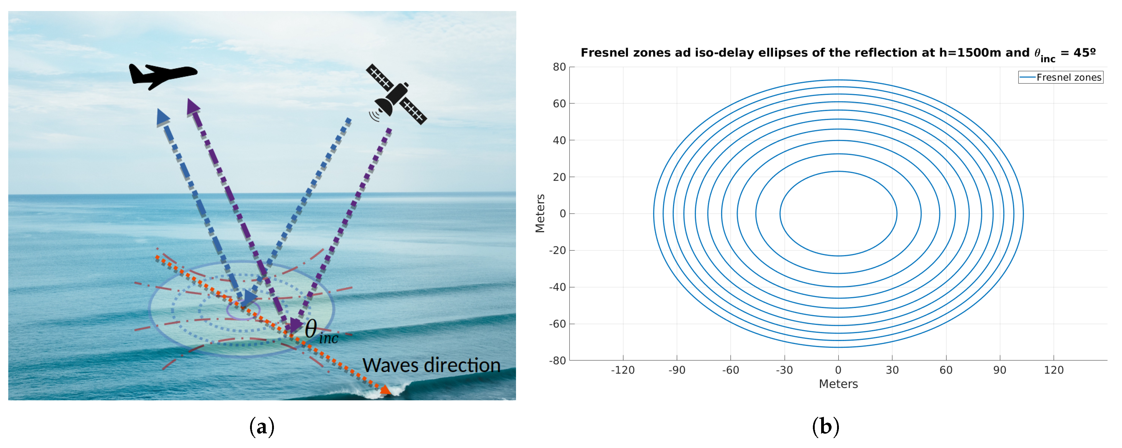
The reflection scenario is illustrated in Figure 4. Note that, the semi-radius of the ellipse formed by the first Fresnel zone [17] (i.e., the area that contains the specular reflection) in the described scenario is limited by the plane altitude as shown in Equation (2).

$$\begin{array}{c}\hfill l_{Fr}={\displaystyle \frac{\sqrt{\lambda R_r}}{cos\left({\theta }_{inc}\right)}},where{R}_r={\displaystyle \frac{h}{cos\left({\theta }_{inc}\right)}}\end{array}$$

(2)

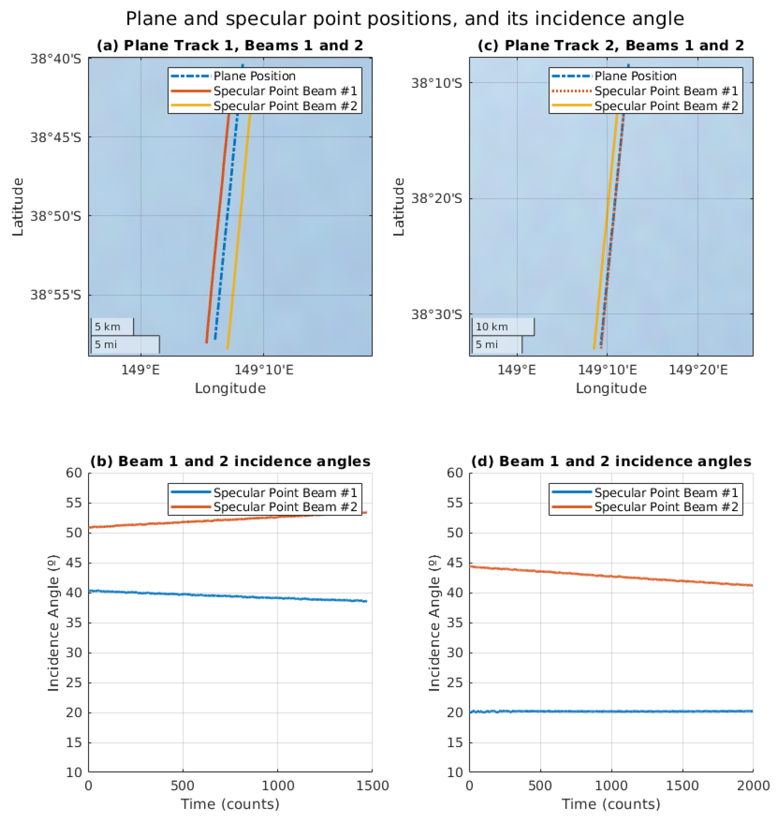
where $\lambda =25$ cm for L5, $h=1500$ m, and ${\theta }_{inc}$ is the wave incidence angle. Therefore, at ${\theta }_{inc}=45°$, $l_{F{r}_{\angle 45}}=33$ m, whereas for an almost-nadir reflection as Beam 1 of Track 2, $l_{F{r}_{\angle 20}}=21$ m.

In this case, second and third reflections occurring in consecutive wave crests in the first Fresnel zone produce different signal wave fronts that are added constructively or destructively in the receiver antenna. However, thanks to the large bandwidth, and hence the very narrow auto-correlation [18] function of the L5/E5a GNSS signal (i.e., 30 m in space), reflections from nearby crests with a distance between them larger than 30 m can produce second peaks in the retrieved waveform.

As an example, two wavefronts are reflected over two successive wave crests, and hence two different specular points, resulting in the addition of the two signals in the receiver antenna, which is detected as a second peak in the processed waveform, as detailed in Figure 5. Sometimes even a third peak appears.

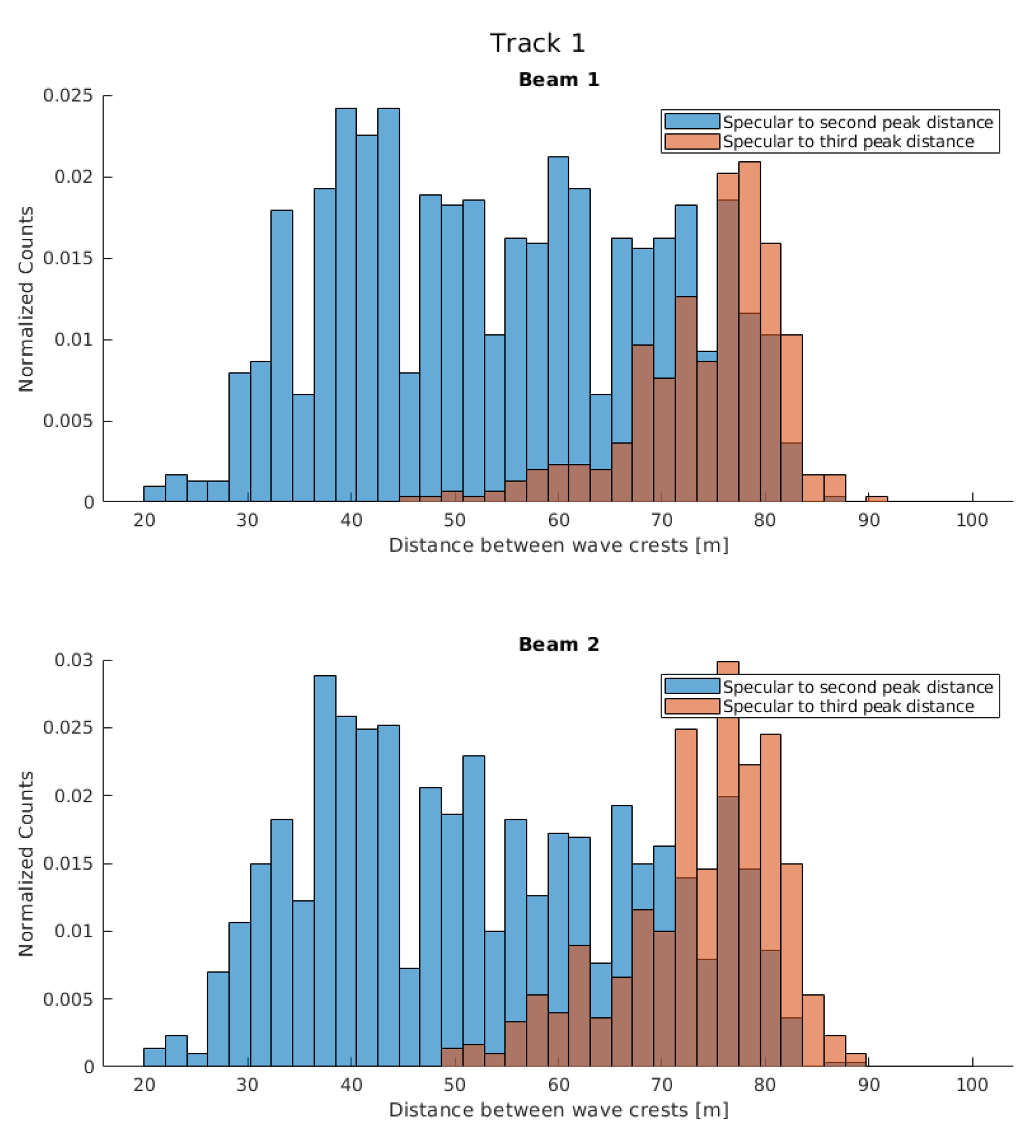
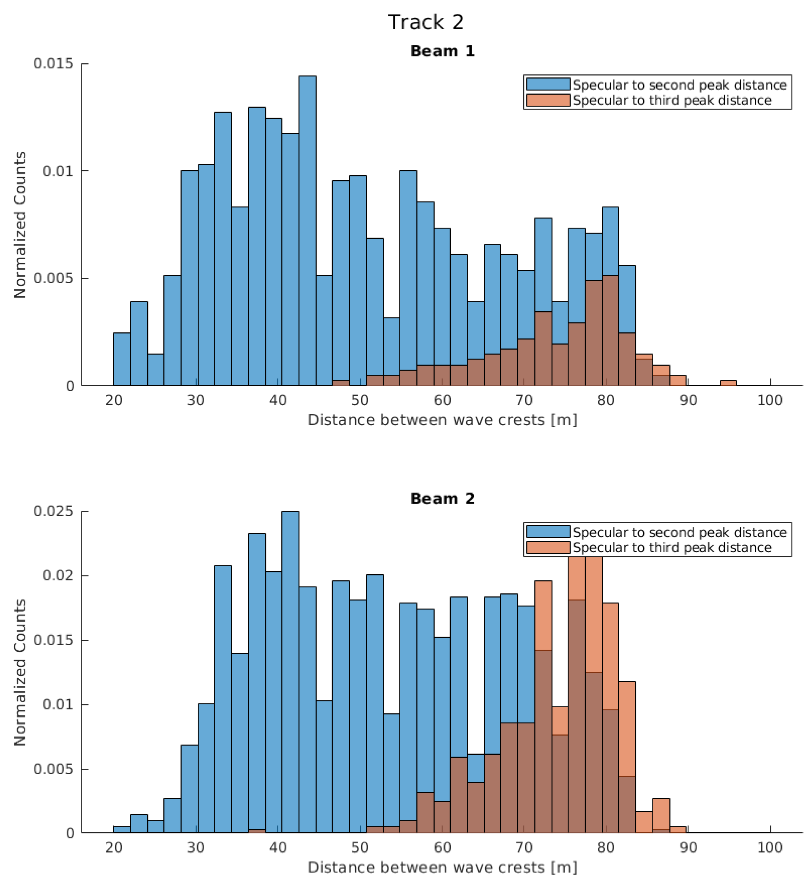
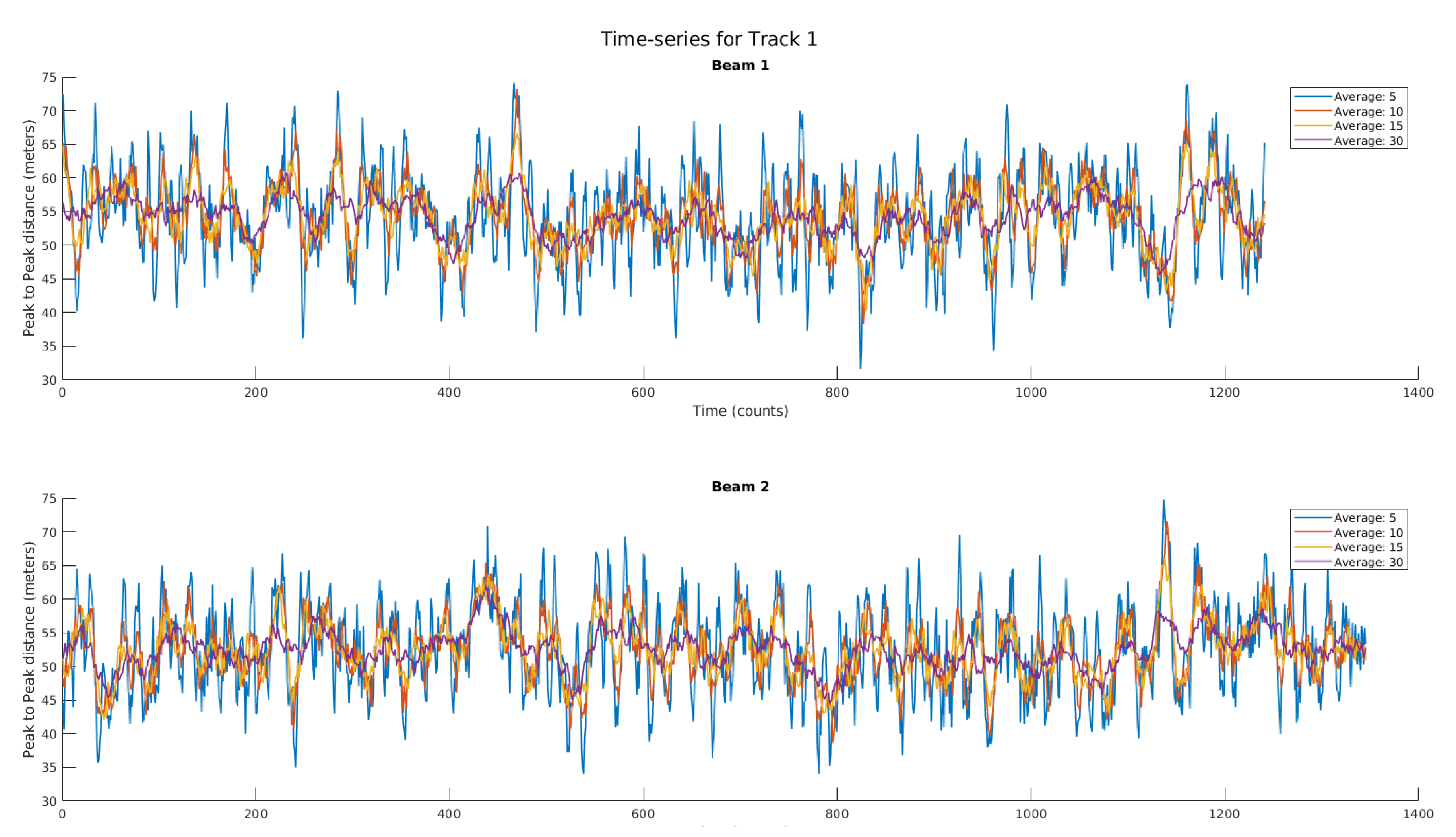
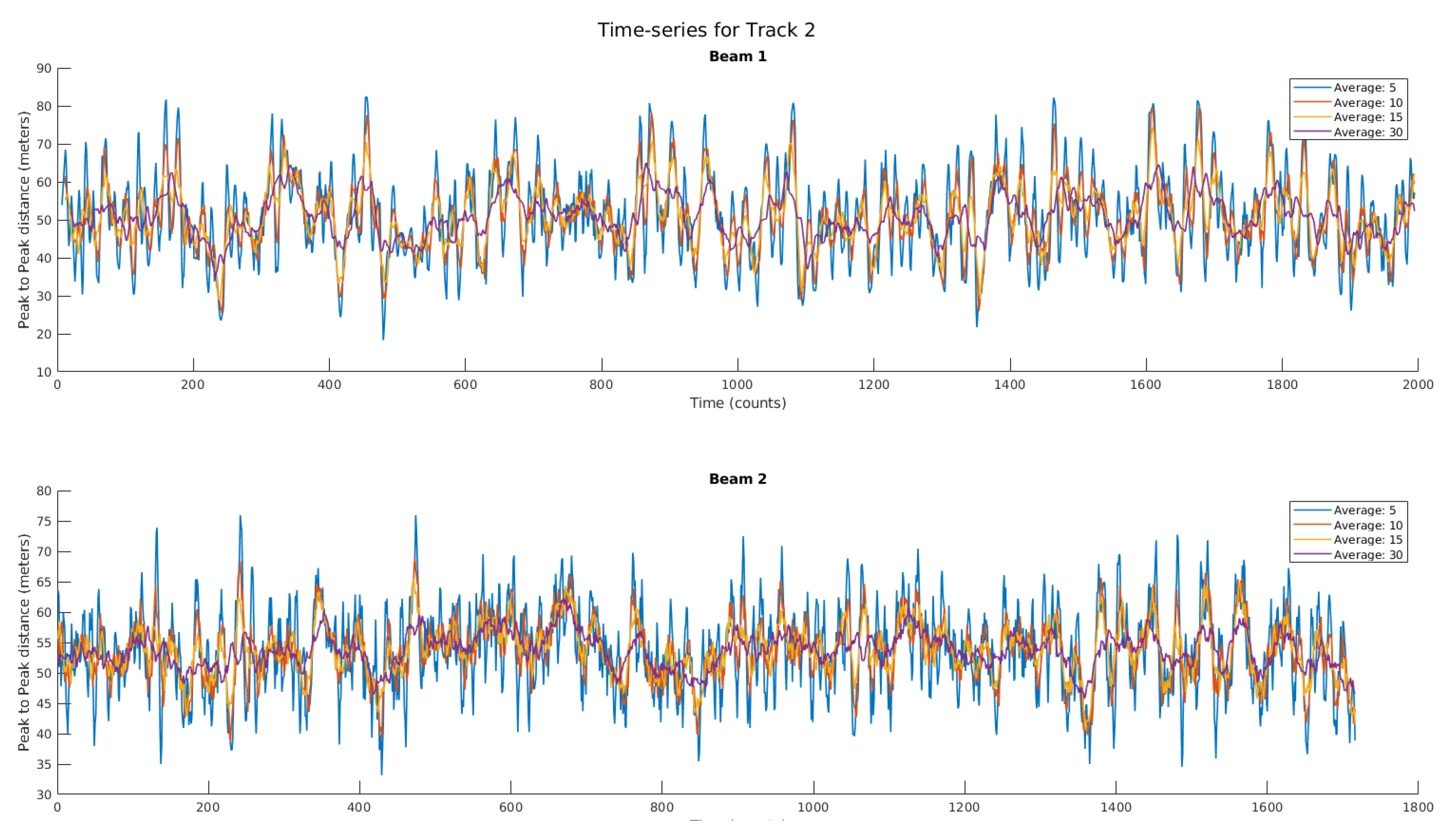
Due to the variability and the surface roughness of the ocean, the distance between two crests varies. In this case, where wind wave and swell wave components are both strong and also with different directions of propagation, the peak-to-peak distance is not preserved from one realization to the next one.

As explained in [19], wind-driven or swell wave period is not a fixed magnitude, but the average of the swell waves component period for the swell waves, and the average of the wind-driven period for the wind-driven waves. As an example, a swell period of 9–10 s generates a larger span of waves, which have a period between them from 8 s to 11 s. Therefore, a relative large data set analysis is required to correctly retrieve the swell waves period or wind-driven waves period.

Finally, the peak-to-peak distance does not only reproduce the crest-to-crest between two consecutive waves, but also a modulation depending on the height between the two waves where the reflection has occurred.

3.1. Waveform Simulation

As opposed to reflections in L1 C/A, where the spatial resolution is mostly limited by the chip length (i.e., 300 m), the new GPS L5 or Galileo E5a signals have 10 times higher spatial resolution, as the auto-correlation function is 10 times narrower (i.e., 30 m in space), allowing de reception of multiple specular points with a distance larger than 30 m. In this case, any reflection from any point separated by more than 30 m produces a secondary peak on the retrieved waveform instead of a blurring on the retrieved wavelength.

This section shows different simulation scenarios of the retrieved waveforms modulated by a forward scattering occurring at the crests of the waves, belonging to different Fresnel zones (Figure 4). To do so, a given PRN of a GPS signal at L5 (${\tau }_{coh}={\tau }_{inc}=1ms$) is sampled at 32.768 MHz (to have better granularity and mimic the MIR sampling ratio) which is then delayed and added as in Equation (3). Note that, due to the sampling used, the distance from the peak to the zero of the auto-correlation (i.e., half the width of the whole auto-correlation function) is ∼3.2 samples.

$$S^{\prime }\left[k\right]=\sum _{i=0}^{N-1}\mathsf{\Phi }\left[i\right]·S[k-i]$$

(3)

where $S^{\prime }\left[k\right]$ is the resulting PRN sequence at the kth sample, sampled at 32.768 MHz, $\mathsf{\Phi }$ is the amplitude coefficient applied to each sample of the clean PRN sequence, S, and N is the length of the $\mathsf{\Phi }$ vector, which represents the reflection scenario, where for this example is set to 10, causing a delay up to three L5 chips.

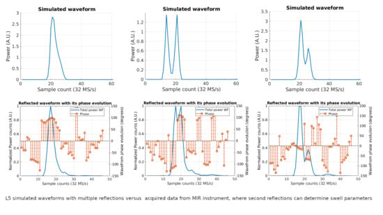
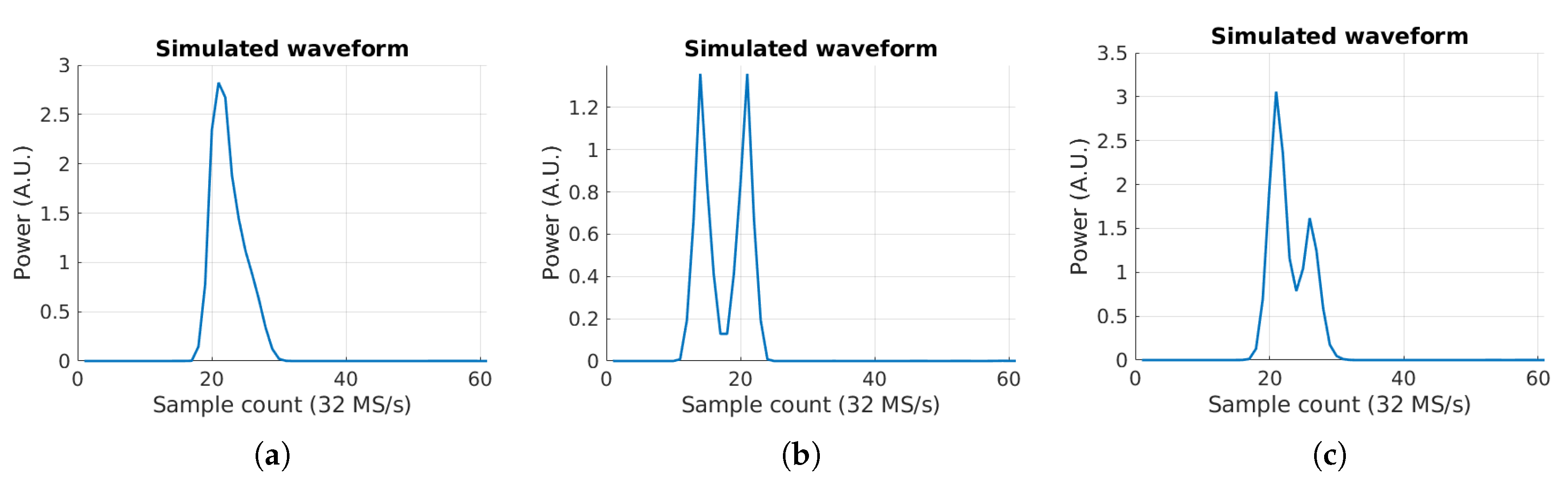
In order to illustrate this concept, three simulated waveforms are computed with different c coefficients. In the first example, using $\mathsf{\Phi }=[1,0.5,0.5,0.4,0.4,0.3,0.3,0.3,0.2,0.1]$ a reflection scenario is computed with lots of small contributions from all the Fresnel zones near the specular point. This produces a waveform as in Figure 6a, where the power decreases, and no secondary peaks are found. However, using $\mathsf{\Phi }=[0.1,1.0,0.1,0.1,0.1,0.1,0.1,0.1,1.0,0.1]$ produces two identical peaks which are easily distinguished. Note that, the separation between the peaks in samples is seven samples. In order to convert the sample distance into a tangible magnitude, the same method as in Equation (10) from [9] is used here in Equation (4).

$${\mathsf{\Delta }}_m={\mathsf{\Delta }}_{samples}·{\displaystyle \frac{c}{f_s}},$$

(4)

where c is the speed of light, $\sim 3·{10}^8$ [m/s], and $f_s$ is the receiver sampling rate, $32.768·{10}^6$ [S/s].

Applying it to Figure 6b, the distance between the two specular reflections (identified as $\mathsf{\Phi }\left[1\right]$ and $\mathsf{\Phi }\left[8\right]$ in previous example), a distance of 64 meters is retrieved.

However, reflections are not always as perfect as in Figure 6b. A third simulation (Figure 6c) is generated using a more realistic case, with $\mathsf{\Phi }=[0.1,0.1,0.4,1.0,0.6,0.1,0.1,0.2,0.8,0.4,0.1,0.1,0.1]$, trying to reproduce two crests separated by five samples or 45 meters. Note that, the amplitudes of the neighbor areas have been also included, but they do not affect the high amplitude specular reflection contribution.

3.2. Evolution of Complex Waveforms in a Single Beam

The previous section has shown three different simulated waveforms synthetically generated to illustrate the concept of a second specular reflection in a consecutive wave crest around the second to sixth Fresnel zones.

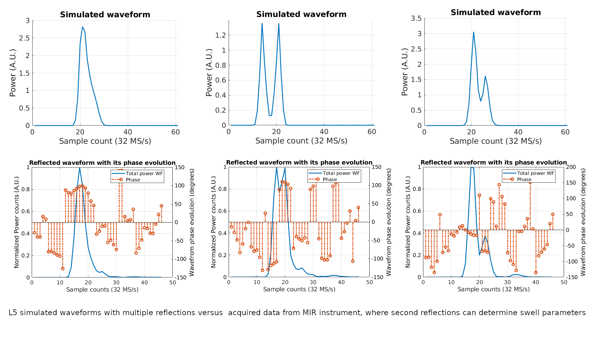
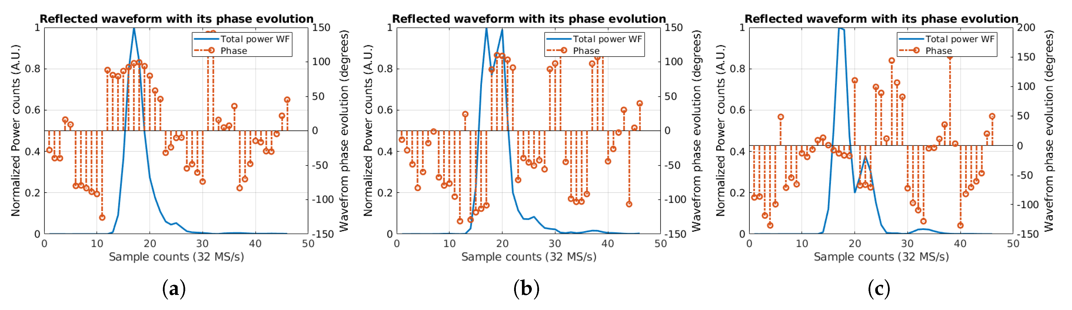
In this section, three consecutive measured waveforms (see Figure 7) have been selected to illustrate these effects. The separation in time between each waveform is 600 ms, and they have been selected because of their similitude to the ones simulated in the previous section. Note that, the three selected waveforms are from Track 1 Beam 1, and both amplitude and phase evolution of the waveform are shown.

The first waveform (Figure 7a) shows an example similar to the one in Figure 6a, where very small contributions from all nearby Fresnel zones causes a blurring of the tail of the waveform.

The main peak is around sample count 17, with a phase approximately constant around +100°. Furthermore, there is a second small peak (in sample 25) around eight samples (i.e., 73 m in space) after the main one (in sample 17). The distance between the peaks indicates that small reflections are coming from the sixth to eighth Fresnel zones.

The second waveform (Figure 7b) shows a example similar to the one in Figure 6b, but with the reflection occurring in a closer Fresnel zone. In this case, the distance between these two peaks is three samples or ∼30 m, which corresponds to a reflection in the second Fresnel zone. Compared to the first waveform, the reflections occurred within the first Fresnel zone causing a blurring and a widening of the L5 auto-correlation function are now split in two different peaks.

As seen, the first peak (in sample 17) has a phase of ∼−110°, and the second peak (in sample 20) has a phase of ∼110° (i.e., close to the phase of the peak in Figure 7b), with a relative phase difference ∼220°, corresponding to reflection in the second Fresnel zone, as both are separated more than 180°. Note that, there is a strong phase jump between the two peaks, indicating that both reflections are coherent (i.e., the phase information is preserved in both cases). As in the previous case, this third peak (in sample count 26) has an approximately constant phase around −50°. In addition and similar to the first waveform, a third small peak is also present nine samples (i.e., 82 m in space) away from the very first one. In this case, the reflection is taking place between the eighth and the tenth Fresnel zones.

Finally, the third waveform (Figure 7c) shows a similar shape as the simulation in Figure 6c, with a relative high second peak (in sample 22) in the reflected waveform which in this case is five samples from the main one (in sample 17). In this last case, the phase evolution is approximately constant in both peaks with a strong jump in the transition between them (i.e., very small incoherent reflection from other Fresnel zones). Note that in this case the relative phase difference is ∼50°, but as the delay in time is ∼45 m, the reflection takes place further away than the second Fresnel zone, the phase with respect to the first peak has advanced at least 180°. Therefore, the absolute phase shift between the two peaks is ∼315°.

3.3. First Waveform Analysis: Determination of the Crest-to-Crest Distance from Peak-to-Peak Distance

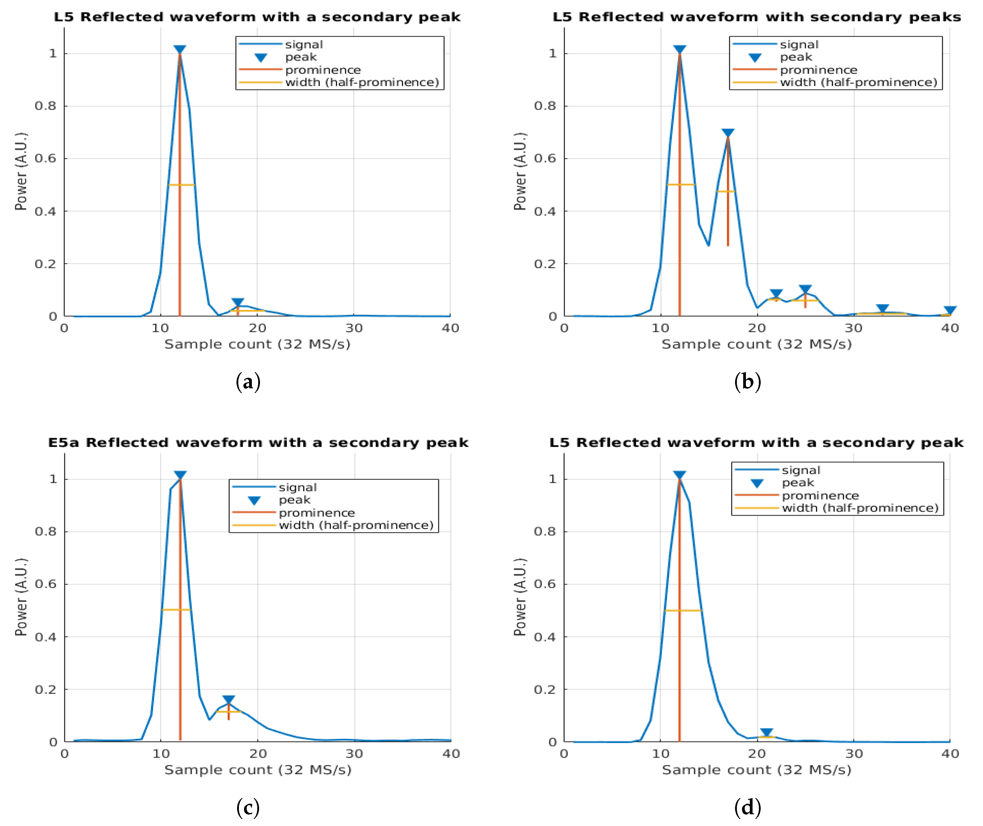
The last section showed three examples of three different waveforms retrieved from Track 1 Beam 1, where the location of the second peak varies with time. Furthermore, it has been shown that this second reflection comes from a different Fresnel zone, and in some cases present a coherent component (i.e., a single specular reflection over a wave crest). Figure 8 illustrates the example of different consecutive peaks present in the GNSS waveforms originated by the forward scattering on two consecutive wave crests, but now in the two beams for the two tracks of the flight.

Note that, the two waveforms for each track (i.e., beams 1 and 2 for Track 1 and beams 1 and 2 for Track 2) are taken at the same moment. As seen, the four waveforms present, at least, one second reflection.

Analyzing each of the tracks, Figure 8a,c present a single second reflection at six samples from the specular one. For the beam 2 case, Figure 8b presents a very large second reflection at six samples from the specular one. In addition, two small reflections are taking place 10 and 13 samples from the specular one. Finally, Figure 8d shows a very low secondary reflection point at nine samples from the main peak.

Applying Equation (4) to the waveform shown in Figure 8, the distance between the peaks in meters are: 54.9 m for both Figure 8a,c, 54.9 m for the first peak of Figure 8b, and 91.5 m for the third peak. Finally for Figure 8d, the distance between the peaks is 82.4 m.

Comparing those retrieved waveforms to the simulated waveforms from Figure 6, it is possible to identify a clear similitude between them, where the second peak (i.e., the one in Figure 8b) reminds the simulated in Figure 6c, due to a specular reflection over a wave crest.

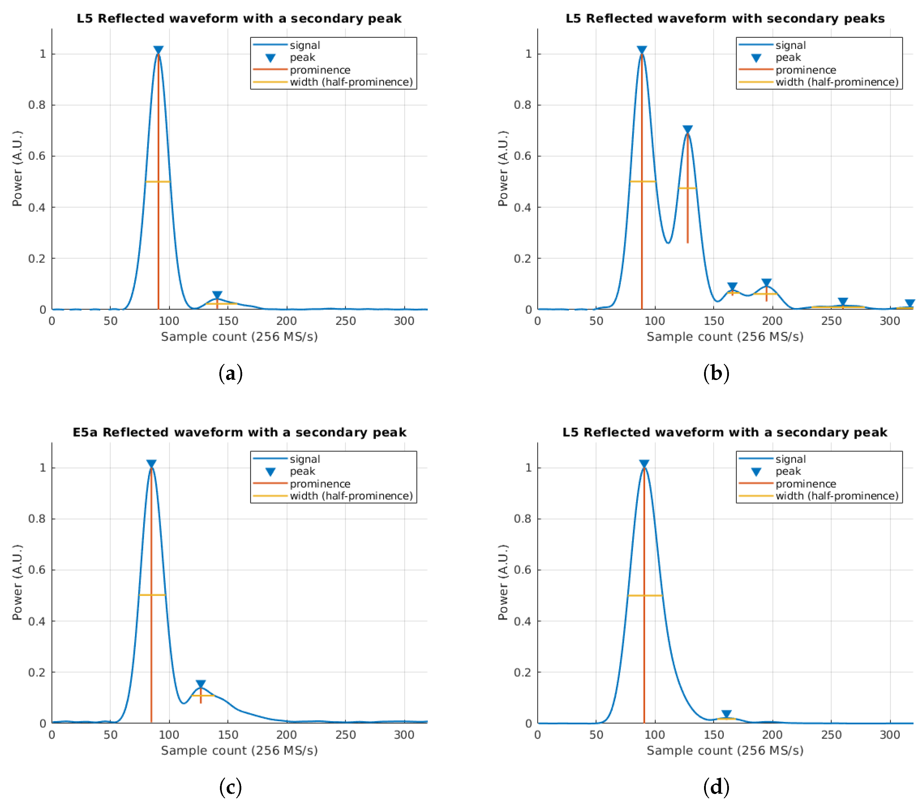
In order to improve the estimations of the separation between peaks in the waveform, since raw data was acquired satisfying the Nyquist criteria at baseband for L5/E5a signals (i.e., $f_s>10$ MHz), therefore the signal can be re-sampled without loss of information. Therefore, waveforms are re-sampled using the Fourier interpolation method (i.e., by inverse FFT of the zero-padded FFT of the waveform), and the local maxima of the interpolated waveform is located. The first two maxima of the waveform are the ones used to retrieve the distance between two consecutive wave crests. The difference in samples between the two peaks position is then converted into meters following the same approach as in previous section, but with a sampling rate $f_s$ scaled by the interpolation rate K.

The selection of this parameter is a trade-off between computational requirements and accuracy when selecting the final position of the multiple peaks. In order to efficiently apply the Fourier interpolation using the Fast Fourier Transform, the signal shall be a multiple of 2, and hence the interpolation rate K, shall be a multiple of 2 as well. In addition, the larger the K parameter is, the lower is the error determination of the peak position of the reflected waveform. For this case an interpolation rate of $K=2$ has a peak position uncertainty of 4.5 meters, and a $K=8$ has a peak position uncertainty of ∼1 m.

In this case, an interpolation rate of $K=8$ has been selected (i.e., now $f_s=256$ MHz). Furthermore, Figure 9 shows the re-sampled version of the waveforms in Figure 8 following the Fourier interpolation method.

The re-sampled versions of the waveforms show a better spatial resolution when estimating the peak-to-peak distance. In this case the distance in samples is: 50, 39, 42, and 70 respectively form (a) to (d). Moreover, the third peak of Figure 9b is located at 77 samples from the specular one.

Applying Equation (4) to the above sample distances, the retrieved crest-to-crest distance (${\mathsf{\Lambda }}_{waves}$) in meters is: 57.2, 44.6, 48, and 80.1 m respectively for (a) to (d), and 88.1 m for the third peak of (b).

Table 2. Track, beam, crest-to-crest estimated distance using the original waveform, and the crest-to-crest distance after re-sampling the original waveform using the FFT interpolation.

Track ID	Beam ID	Original Crest-to-Crest Distance [m]	Re-Sampled Crest-to-Crest Distance [m]
1	1	54.5	57.2
1	2	54.5	44.6
2	1	54.5	48.0
2	2	82.4	80.1

compares the values prior to the re-sampling with the re-sampled values. Note that, the estimation of both the first peak position is enhanced thanks to the FFT interpolation. In addition, the estimation of the position of the second peaks is also enhanced. A proper estimation of the position of both peaks is crucial to better determine the distance between the two reflections (i.e., the two wave crests). Note the difference in Beam 2 of Track 1 and Beam 1 of Track 2, where the first approach does not show the proper crest-to-crest distance, introducing an error of almost 10 m in the measurement.

This section has covered the simulation and its comparison with real data of different scenarios where different specular reflections are generating second and even third peaks on the reflected waveform. The study on the phase evolution in this secondary peaks shows that the second reflection is coherent, and hence is coming from a different specular point, as was detailed in Figure 5. Finally, the use of FFT interpolation enhances the determination of the peak-to-peak distance, showing a better granularity when determining this magnitude.

4. Sea Wavelength Retrieval Using Large Data Set

The study of a larger data set is required to validate the relationship between sea waves wavelength ${\mathsf{\Lambda }}_{waves}$ or wave period $T_{waves}$ to the distance between the peaks in the waveforms. Tracks identified in Table 1 of Section 2 are composed by 1470 waveforms, and 1994 waveforms respectively, generated once per 30 ms (i.e., 3.33 Hz), which corresponds to ∼8 min of data for each of the two beams for the first track, and 11 minutes of data for the second track. In order to analyze the data set, three different approaches are considered:

• Statistical analysis: statistics of the retrieved crest-to-crest distance and presence or not of third peaks.
• Time-series analysis: analysis in the time domain of the retrieved crest-to-crest distance.
• Spectral analysis: analysis in the frequency domain of the time-series data.

4.1. Statistical Analysis

Reviewing the histogram of all the 1470 measurements for Track 1 (see Figure 10), most of the results are condensed between 30 m (the wind-driven wavelength from the model is 39 m) and 80 m (the swell wavelength from the model is 126 m).

In addition, the distance to a third peak (if is exists) is condensed just at the end of the histogram, at the end of the histogram of the distance to the second peak. As seen, the measurements are condensed mostly between 40 and 90 m for both beams.

Both beams are following similar statistics for the second peak distance, with an average value of 54.3 m for Beam 1, and an average value of 52.6 m for Beam 2. The third peak has an average value of 74.5 m for Beam 1, and 73.5 m for Beam 2. Note that, the average of the measurements is a mixture of all possible wave crest distance contributions. Note that, the least wave crest distance is $\sim 30$ m, which coincides with the spatial resolution due to the chip bandwidth of the L5/E5a signal, 30 m.

In addition, the same histogram of the second-track is shown in Figure 11. The first beam corresponds to a Galileo E5a signal, which has an incidence angle of ∼20°. The mean peak-to-peak distance in this case is 50.8 m. The second beam has an incidence angle of 42°, with an average value of 53.5 m.

In case of this first beam, as the incidence angle is lower, the semi-radius of the first Fresnel zone is smaller (from 33 m with ${\theta }_{inc}=45°$ to 21 m with ${\theta }_{inc}=20°$). As the overall sizes of the Fresnel zones are smaller, the area where the possible strong reflection occurs over a wave crest is also smaller, hence some waves with a large distance between them can not be captured.

Note that, in this case, the third peak position for Beam 1 is poorly determined because of the small incidence angle, and the size of the Fresnel zones for that case. As seen in the histogram, the amount of third peak reflections in Beam 1 with respect to Beam 2 is in the order of 0.25.

As seen in the two tracks, the histogram analysis shows that multiple reflections are present in most of the waveforms, with an average value ∼50 m for the distance between the first two peaks. From this first analysis, the wind-driven waves wavelength can be estimated (i.e., the model set this distance to 40 m), and from it the wind-driven wave period.

4.2. Time-Series Analysis

The statistical analysis through the histogram visualization shows that the crest-to-crest distances are in the same range than in the ICON model (Section 2), the analysis of the time evolution of the peak-to-peak distances shows a wavy behavior.

In order to reduce the noise of the measurement, four different averaging windows have been applied to the peak-to-peak distance. In this case, the averaging selected is 5, 10, 15, and 30 samples. As seen in Figure 12, this wavy behavior is clearly identified in the measurement, which is present even with large averaging windows. As seen with the highest averaging time, the mean of the crest-to-crest distance is ∼55 m for Beam 1, and ∼52.5 m for Beam 2. As seen in [14,19], the average wave period, or the average wavelength, ${\mathsf{\Lambda }}_{waves}$, tends to the combination of all the different wave contributions.

A similar behavior is also found in Track 2, as shown in Figure 13. The Galileo signal (i.e., Beam 1), has a mean value ∼50 m, and Beam 2 a mean value on the order of $\sim 52.5$ m, as in Track 1. Note that, a large portion (∼ 40%) of the Beam 1 reflections do not have a secondary peak because of the reflection geometry. As the incidence angle is very close to 0° (i.e., very close to nadir), the possible reflections are coming from closer wave crests, therefore the receiver is only able to infer consecutive crests which are closer one to each other.

4.3. Spectral Analysis

The time-series analysis together with the statistical one show that there is a vast range of retrieved sea wave wavelengths ${\mathsf{\Lambda }}_{waves}$, with some apparent periodicity. As detailed in [12,14], a spectral analysis over the magnitude under study helps to separate the different swell or wind-driven wave contributions.

In order to do that, the power spectral density of the time-series data from previous section is computed. Figure 14 shows the power spectral density of the distance to the second peak (or the first encountered crest in the sea wave surface). In all four figures, there are some common frequencies at ∼0.06 Hz, 0.1 Hz, 0.15 Hz, and also a 0.2 Hz component in Beam 1 of both Tracks 1 and 2.

Converting those frequencies to seconds, the wave periods of each of the wavelengths are $T_1=$ 16.6 s, $T_2=$ 10 s, and $T_3=$ 6.66 s. Comparing the three periods to the swell and wind-driven wave periods to the ones of the ICON model in Figure 2, $T_2\simeq T_{swell}$ and $T_3\simeq T_{wind}$.

In addition, the 0.2 Hz component, corresponding to a period of $T_4=$ 5 s, which is only present in Beam 1 of both Track 1 and Track 2, exactly matches the wind-driven prediction by the model, where $T_{wind}=$ 5 s.

As already stated, the lower the incidence angle of the beam, the shorter waves can be retrieved (i.e., waves with shorter period), which is mostly the case for Figure 14c, where the incidence angle is closer to 0° (i.e., nadir), and hence wind-wave periods can be retrieved rather than swell-driven wave periods.

Furthermore, in case of analyzing the power spectral density (Figure 15) for the distance to the third peak, the fundamental frequencies are below the previous case, with a first fundamental frequency consistent in (a), (c), and (d) around ∼0.03 Hz, 33 s of period.

The spectrum shape of this third peak indicates a long period sea wavelength which is not contemplated in the model. As stated in [19], this high order period is present on swell waves, and also modulates the amplitude of the swell waves, it is known as second swell.

In this case, the third peak spectrum does not give as much information as the second peak, from where it is possible to infer the wave period for different wave sources, as swell, wind-driven wind, or secondary swell waves.

5. Discussion

Each analysis provides a different perspective and hence a different parameter of the ocean can be estimated, and they are all summarized and compared to the values predicted by the ICON model in

Table 3. Estimated wave period from the three different analysis applied and its comparison ot the ICON model prediction.

Measurement	Est. Wave Period	ICON Model Estimation
Statistical analysis	5.8 s	Wind-driven = 5 s Swell = 9 s
Time-series analysis	5.6 s	Wind-driven = 5 s Swell = 9 s
Spectral analysis	Four components: 5 s, 6.3 s, 10 s, 16.6 s	Wind-driven = 5 s Swell = 9 s

. Note that, the wave periods in the statistical and time-series approaches have been determined from the average crest-to-crest distance and assuming ${\mathsf{\Lambda }}_{waves}=1.56·T_{waves}^2$, as in (1).

In this case, both the statistical and the time-series analysis are providing a good estimation of the wind-driven wavelength, as the period of the wind-driven waves is smaller, the amount of wave crests per unit of area is larger, and hence the mean value of the waves is biased towards the wind-driven waves.

It is also important to remark that the time analysis serves to illustrate the wavy behavior of the crest-to-crest distance with respect to time. In this case, this analysis shows in a qualitative way how crest-to-crest distance is a mixture of different components, as explained in [12,14].

Last but not least, the spectral analysis clearly shows the different periods that can be identified in the time analysis. Multiple periods can be identified, among them ${\tau }_{swell}$ and ${\tau }_{wind}$ are identified as the main components of the spectrum of the crest-to-crest distance.

Furthermore, the results from the spectral analysis and the statistical analysis confirm that due to the geometry of the reflection, the lower the incidence angle is, the closer the reflection of the second crest occurs.

Finally, the spectral analysis also shows very low frequency components due to secondary swell or high period gravitational waves, which are interesting for other oceanographic studies, but still need further investigation.

6. Conclusions

This work has presented the first experimental evidence of wind and swell waves signatures in L5/E5a GNSS-R waveforms from second and third peaks. An algorithm has been presented to retrieve the peak-to-peak distance. Evidences for both the first and the second peaks are presented, and a detailed analysis from a large data set $N>1000$ waveforms has been presented. The analysis in three domains (statistical, time, and spectrum) shows that additional ocean parameters can be retrieved from GNSS-R measurements, e.g., wind driven waves period and swell period, which have not been measured yet using GNSS-R technique.

This application still requires further refinements and a more exhaustive analysis with in-situ data. However, this study shows the promising results for the use of L5/E5a GNSS-R signals to infer new geophysical parameters as the wave period or wavelength of the sea thanks to the sharper shape of the auto-correlation function.

References

1. Zavorotny, V.U.; Gleason, S.; Cardellach, E.; Camps, A. Tutorial on Remote Sensing Using GNSS Bistatic Radar of Opportunity. IEEE Geosci. Remote. Sens. Mag. 2014, 2, 8–45. [Google Scholar] [CrossRef] [Green Version]
2. Onrubia, R.; Pascual, D.; Park, H.; Camps, A.; Rüdiger, C.; Walker, J.; Monerris, A. Satellite Cross-Talk Impact Analysis in Airborne Interferometric Global Navigation Satellite System-Reflectometry with the Microwave Interferometric Reflectometer. Remote. Sens. 2019, 11, 1120. [Google Scholar] [CrossRef] [Green Version]
3. Onrubia, R.; Pascual, D.; Park, H.; Camps, A. Preliminary Altimetric and Scatterometric Results with the Microwave Interferometric Reflectometer (MIR) during Its first Airborne Experiment; ARSI-KEO 2019; ESA: Noordwijk, The Netherlands, 2019.
4. Bathgate, J.S.; Heron, M.L.; Prytz, A. A Method of Swell-Wave Parameter Extraction From HF Ocean Surface Radar Spectra. IEEE J. Ocean. Eng. 2006, 31, 812–818. [Google Scholar]
5. Chen, Z.; Zhang, L.; Zhao, C.; Chen, X. Wind sea and swell meansurements using S-band Doppler radar. In Proceedings of the OCEANS 2016, Shanghai, China, 19–23 September 2016; pp. 1–5. [Google Scholar]
6. Johnsen, H.; Husson, R.; Vincent, P.; Hajduch, G. Sentinel-1 Ocean Swell Wave Spectra (OSW) Algorithm Definition; Northern Research Institute (Norut): Tromso, Norway, 2020. [Google Scholar]
7. Robinson, I.S. Measuring the Oceans from Space: The Principles and Methods of Satellite Oceanography; Springer: Berlin, Germany, 2004. [Google Scholar]
8. Ward, K.D.; Tough, R.J.A.; Watts, S. Sea clutter: Scattering, the K distribution and radar performance. Waves Random Complex Media 2007, 17, 233–234. [Google Scholar] [CrossRef]
9. Munoz-Martin, J.F.; Onrubia, R.; Pascual, D.; Park, H.; Camps, A.; Rüdiger, C.; Walker, J.; Monerris, A. Untangling the Incoherent and Coherent Scattering Components in GNSS-R and Novel Applications. Remote. Sens. 2020, 12, 1208. [Google Scholar] [CrossRef] [Green Version]
10. (DWD), D.W. ICON model description by DWD. Available online: https://www.dwd.de (accessed on 7 January 2020).
11. US Army Corpsof Engineers. Coastal Engineering Manual Part II: Coastal Hydrodynamics (EM 1110-2-1100); Books Express Publishing: Newbury Berkshire, UK, 2012.
12. Wang, D.W.; Hwang, P.A. An Operational Method for Separating Wind Sea and Swell from Ocean Wave Spectra. J. Atmos. Ocean. Technol. 2001, 18, 2052–2062. [Google Scholar] [CrossRef]
13. Portilla, J.; Ocampo-Torres, F.J.; Monbaliu, J. Spectral Partitioning and Identification of Wind Sea and Swell. J. Atmos. Ocean. Technol. 2009, 26, 107–122. [Google Scholar] [CrossRef]
14. Hwang, P.A.; Ocampo-Torres, F.J.; García-Nava, H. Wind Sea and Swell Separation of 1D Wave Spectrum by a Spectrum Integration Method. J. Atmos. Ocean. Technol. 2012, 29, 116–128. [Google Scholar] [CrossRef]
15. InMeteo. Ventusky. Available online: https://ventusky.com (accessed on 7 January 2020).
16. Voronovich, A.G.; Zavorotny, V.U. The Transition From Weak to Strong Diffuse Radar Bistatic Scattering From Rough Ocean Surface. IEEE Trans. Antennas Propag. 2017, 65, 6029–6034. [Google Scholar] [CrossRef]
17. Giacobazzi, J. 50 - Line of sight radio systems. In Telecommunications Engineer’s Reference Book; Mazda, F., Ed.; Butterworth-Heinemann: Oxford, UK, 1993; pp. 50-1–50-17. [Google Scholar] [CrossRef]
18. Saleem, T.; Usman, M.; Elahi, A.; Gul, N. Simulation and Performance Evaluations of the New GPS L5 and L1 Signals. Wirel. Commun. Mob. Comput. 2017, 2017, 1–4. [Google Scholar] [CrossRef] [Green Version]
19. Government, A. Waves. Available online: http://www.bom.gov.au/marine/knowledge-centre/reference/waves.shtml (accessed on 14 March 2020).
Figure 1. (a) Microwave Interferometric Reflectometer (MIR) instrument and up-looking array mounted inside the airplane, and (b) down-looking array covered with a radome hanging from the airplane’s fuselage [2].
Remotesensing 12 01759 g001
Figure 2. Position of the plane superposed to (a) wind-driven wave period, (b) swell wave period, and (c) wind speed over sea of the data used for the secondary specular reflection analysis. The plane trajectories framed in white box is zoomed in Figure 3. The wind-driven period, the swell period, and the wind speed are provided below the white box [15]
Remotesensing 12 01759 g002
Figure 3. Top frame—plane position and specular point position of Track 1 (a) and Track 2 (c). Bottom frame—incidence angle to the specular point of Track 1 (b) and Track 2 (d). The plane positions correspond to the white frame box in Figure 2. Note that, the plane position and specular point of Beam 1 of Track 2 are superposed due to the very low incidence angle (i.e., almost nadir).
Remotesensing 12 01759 g003
Figure 4. (a) An example of the reflection scenario, where two wavefronts are reflected over two consecutive wave crests, where θ i n c is the incidence angle of the reflected signal. (b) The first 10 Fresnel zones associated to the reflection scenario described in (a), computed at θ i n c = 45 °. Note that each Fresnel zone corresponds to a 180° phase rotation.
Remotesensing 12 01759 g004
Figure 5. Forward scattering over two wave crests.
Remotesensing 12 01759 g005
Figure 6. Three simulated waveforms different contributions from nearby Fresnel zones, producing secondary peaks driven by strong specular and coherent reflections over two hypothetical consecutive wave crest. (a) Simulated waveform with small contributions from all the nearby Fresnel zones, (b) simulated waveform with two ideal peak reflections separated by seven samples, and (c) simulated waveform with realistic contributions from a secondary strong reflection separated by five samples.
Remotesensing 12 01759 g006
Figure 7. Three sample waveforms containing different contributions from different Fresnel zones, producing secondary peaks with different shapes. (a) Retrieved waveform with small contributions from all the nearby Fresnel zones, (b) retrieved waveform with two big peaks of the same amplitude separated three samples one from other, and (c) retrieved waveform with two peaks with different amplitudes and separated by five samples.
Remotesensing 12 01759 g007
Figure 8. Reflected waveform for (a) Track 1, Beam 1; (b) Track 1, Beam 2; (c) Track 2, Beam 1; and (d) Track 2, Beam 2 of GPS L5 and Galileo E5a signals over the sea surface with an incoherent integration time of 40 ms.
Remotesensing 12 01759 g008
Figure 9. Reflected waveforms for (a) Track 1, Beam 1; (b) Track 1, Beam 2; (c) Track 2, Beam 1; and (d) Track 2, Beam 2 from Figure 8 now sampled at 256 MHz. Note that, thanks to the re-sampling the determination of the peak position is enhanced.
Remotesensing 12 01759 g009
Figure 10. Histogram of the peak-to-peak distances for Track 1. Top figure corresponds to Beam 1 (GPS L5) and bottom figure to Beam 2 (GPS L5).
Remotesensing 12 01759 g010
Figure 11. Histogram of the peak-to-peak distances for Track 2. Top figure corresponds to Beam 1 (Galileo E5a) and bottom figure to Beam 2 (GPS L5).
Remotesensing 12 01759 g011
Figure 12. Time-series evolution of the Track 1 peak-to-peak calibrated distance with different moving average windows. Top figure corresponds to Beam 1, and bottom figure to Beam 2.
Remotesensing 12 01759 g012
Figure 13. Time-series evolution of the Track 2 peak-to-peak calibrated distance with different moving average windows. Top figure corresponds to Beam 1, and bottom figure to Beam 2.
Remotesensing 12 01759 g013
Figure 14. Fourier Transform of the time series evolution of (Figure 12 and Figure 13), for the second peak distances.
Remotesensing 12 01759 g014
Figure 15. Fourier Transform of the time series evolution of (Figure 12 and Figure 13), for the third peak distances.
Remotesensing 12 01759 g015