Deep Learning-Based Single Image Super-Resolution: An Investigation for Dense Scene Reconstruction with UAS Photogrammetry

Abstract

The deep convolutional neural network (DCNN) has recently been applied to the highly challenging and ill-posed problem of single image super-resolution (SISR), which aims to predict high-resolution (HR) images from their corresponding low-resolution (LR) images. In many remote sensing (RS) applications, spatial resolution of the aerial or satellite imagery has a great impact on the accuracy and reliability of information extracted from the images. In this study, the potential of a DCNN-based SISR model, called enhanced super-resolution generative adversarial network (ESRGAN), to predict the spatial information degraded or lost in a hyper-spatial resolution unmanned aircraft system (UAS) RGB image set is investigated. ESRGAN model is trained over a limited number of original HR (50 out of 450 total images) and virtually-generated LR UAS images by downsampling the original HR images using a bicubic kernel with a factor $\times 4$. Quantitative and qualitative assessments of super-resolved images using standard image quality measures (IQMs) confirm that the DCNN-based SISR approach can be successfully applied on LR UAS imagery for spatial resolution enhancement. The performance of DCNN-based SISR approach for the UAS image set closely approximates performances reported on standard SISR image sets with mean peak signal-to-noise ratio (PSNR) and structural similarity (SSIM) index values of around 28 dB and 0.85 dB, respectively. Furthermore, by exploiting the rigorous Structure-from-Motion (SfM) photogrammetry procedure, an accurate task-based IQM for evaluating the quality of the super-resolved images is carried out. Results verify that the interior and exterior imaging geometry, which are extremely important for extracting highly accurate spatial information from UAS imagery in photogrammetric applications, can be accurately retrieved from a super-resolved image set. The number of corresponding keypoints and dense points generated from the SfM photogrammetry process are about 6 and 17 times more than those extracted from the corresponding LR image set, respectively.

1. Introduction

In most remote sensing (RS) applications, high-resolution (HR) images are usually more demanding in a wide range of image analysis tasks leading to more precise and accurate RS-derived products [1,2,3]. HR imagery is usually more desirable in all applications, including RS imagery, because improved pictorial information makes visual interpretation easier for a human and helps to purify representation for automatic machine perception [4]. In RS applications, the resolution of a digital imaging system can be classified in four different ways: spatial resolution, spectral resolution, radiometric resolution, and temporal resolution. In the context of accurate feature mapping and positioning in RS, spatial resolution is of the greatest challenge.

Spatial resolution of a digital imaging system is primarily defined by the pixel density in the image space, which is measured in pixels per unit area. Spatial resolution in the object space represents the level of spatial detail that can be discerned in an image; the higher the resolution, the more image details. Limited spatial resolution in a certain image is primarily a function of the imaging sensor or acquisition device [4]. The spatial resolution of imagery, usually referred to as ground sample distance (GSD) in RS applications, is determined by the sensor size or the dimension of the electro-optical sensor when based on the charge-coupled device (CCD) or complementary metal-oxide-semiconductor (CMOS) technologies, the number of sensor elements, the focal length of the imaging device, and its distance from the imaging target. Regardless of the other factors contributing to the spatial resolution of imagery, such as focal length and the distance from sensor to the target, GSD of an image and the quality of its high-frequency contents deteriorate mainly due to some manufacturing limitations and imperfections of an imaging sensor.

One straightforward way to improve the spatial resolution or GSD of imagery is to build a more compact sensor in which the sensor’s pixel density is increased by reducing the sensor element size. However, this reduction in sensor element size may dramatically reduce the amount of light incident on each sensor element, causing the so called shot noise [5]. Furthermore, capture of high frequency image detail is also limited or degraded by the sensor optics, such as lens blur, lens aberration, and aperture diffraction, or any external sources of image degradation including image motion due to moving objects [4]. Constructing high-quality imaging sensors with perfect optical components, capturing very high spatial resolution images with high-quality image content, is restrictively expensive and not practical in most real scenarios. This is especially true when referring to the rapid rise in the use of small unmanned aircraft systems (UASs) for RS and photogrammetry applications [4]. Such small UASs are typically equipped with low-cost, consumer-grade digital RGB cameras. Besides the cost, the resolution of these typical UAS cameras is also limited by the camera speed and hardware storage. Physical constraints of the sensing platform or environment, such as with satellite imagery, can put additional constraints on the use of very high-resolution sensors. Furthermore, in some imaging systems, HR image content may not be always achievable due to inherent restrictions within the system itself including built-in downsampling procedures to handle bandwidth limitations, different types of noise related to the sensor electronics and atmosphere, compression techniques, etc. [6].

An alternative approach to hardware-based solutions for spatial resolution enhancement is to accept the image degradation and apply signal processing techniques to attempt to recover fine image details degraded or almost lost during image capture. These approaches are often referred to as Super-Resolution (SR) image reconstruction techniques. SR techniques attempt to recover HR images from LR images, and this task remains an important yet challenging topic in image processing that has a wide range of applications in computer vision and image understanding tasks [7,8,9,10]. SR techniques not only improve image perceptual quality, but also help to improve the final accuracy of many computer vision tasks [11,12,13]. Application of SR techniques on highly detailed and complex RS data introduces more challenges to the SR problem [14,15]. Most traditional image SR techniques use highly sophisticated signal processing algorithms with a very high computational complexity [15,16]. Considering the size and the volume of required super-resolved images for some RS applications, such as generating a precise digital surface model (DSM) using aerial or satellite photogrammetry, traditional SR techniques are highly inefficient for such applications. Furthermore, some techniques require multiple LR images from the same scene with high temporal resolution to resolve the SR problem [17,18]. However, due to costs or limitations for acquiring the necessary imagery, complexity of natural and built terrain, scarcity of multi-view sensors, and need for accurate image registration algorithms, acquiring and processing such images for SR is a difficult task [15]. In addition, complicated and versatile interaction of most RS sensors with atmosphere and objects, image displacements due to topographic anomalies, land cover characteristics, and participation of shaded areas due to the Sun-sensor-object geometry in RS images make the SR problem a highly challenging task for almost all developed techniques in this field [15].

Deep learning (DL), specifically deep convolutional neural network (DCNN), has recently been applied to a wide range of image analysis tasks [19,20,21,22] including the highly challenging and ill-posed problem of predicting HR images from LR images in an end-to-end manner. These methods have already shown their superiority over almost all traditional techniques by achieving state-of-the-art performance on various SR benchmarks [23,24,25]. Currently, DCNN-based single image super-resolution (SISR) techniques have been employed to increase the geometrical and interpretation quality of RS imagery [26,27,28]. However, few studies have focused on applying DCNN-based SISR on UAS-based imagery, typically acquired at low altitudes with high resolution, where the accuracy of the spatial information captured by the images is critical for the reliability of results drawn from subsequent analyses [29,30]. Recently, super-resolution generative adversarial network (SRGAN) [23], is considered as one of the most efficient DCNN-based SISR models for recovering very fine details in predicted HR images from corresponding LR images [23]. Offering finer image content is always one of the most important characteristics of HR images in different RS applications, which can lead to higher accuracy and reliability in almost all spatial and non-spatial RS products. SRGAN has already proved its superiority over many other DCNN-based SISR models for recovering very fine details in predicted HR images, which are highly valuable for improving human image perception. However, the quality of the recovered image details and their potential for enhancement of hyper-spatial resolution UAS imagery for photogrammetric applications, such as dense 3D reconstruction of a scene, has not yet been fully explored. With this motivation, this paper focuses on the application of DCNN to SISR for UAS image enhancement. The contributions of the paper are as follows:

• An overview of the SR problem and DCNN approaches for SISR is provided with emphasis on generative adversarial network (GAN) architecture. GAN-based models are fully reviewed including their specific loss functions. Additionally, different learning strategies and image quality measures (IQMs) typically employed for SISR tasks are reviewed.
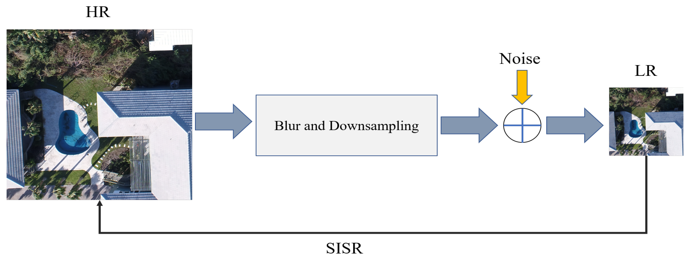
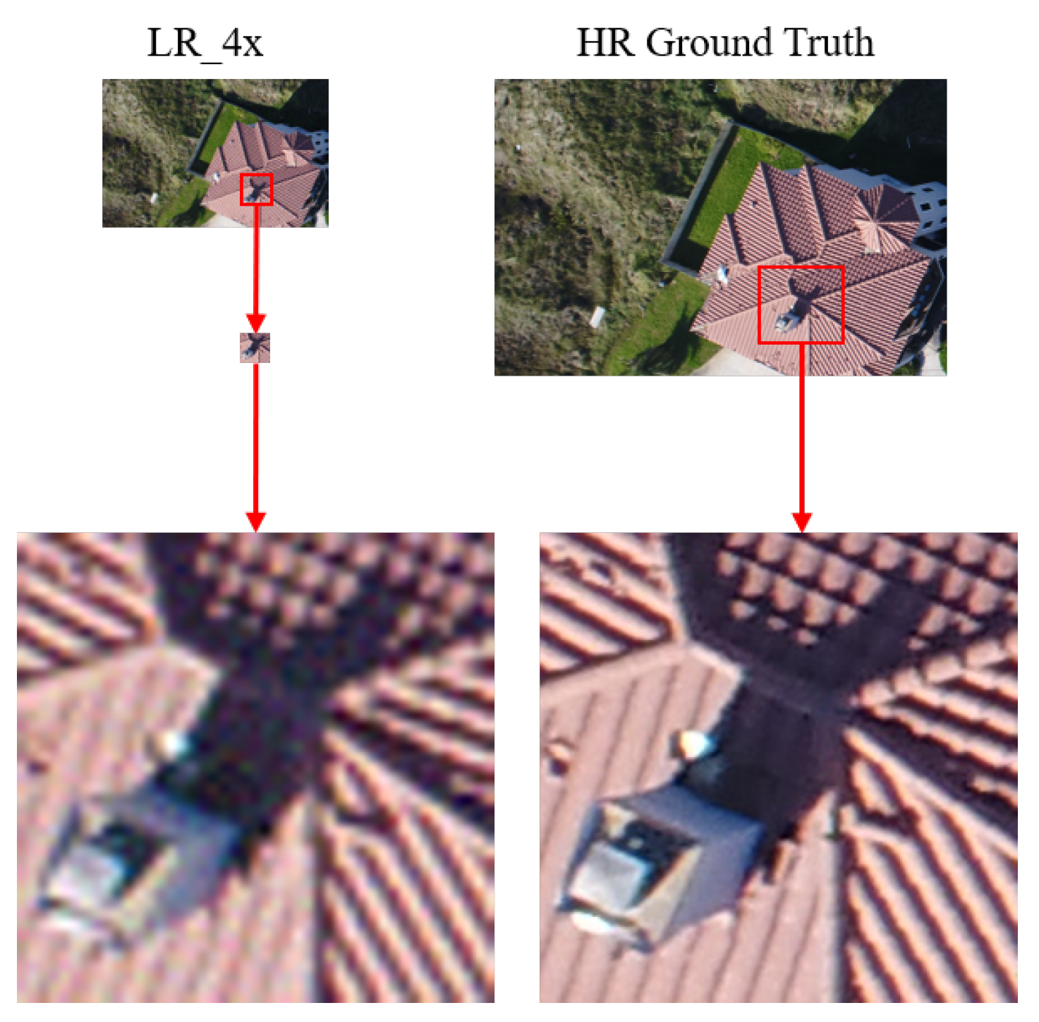
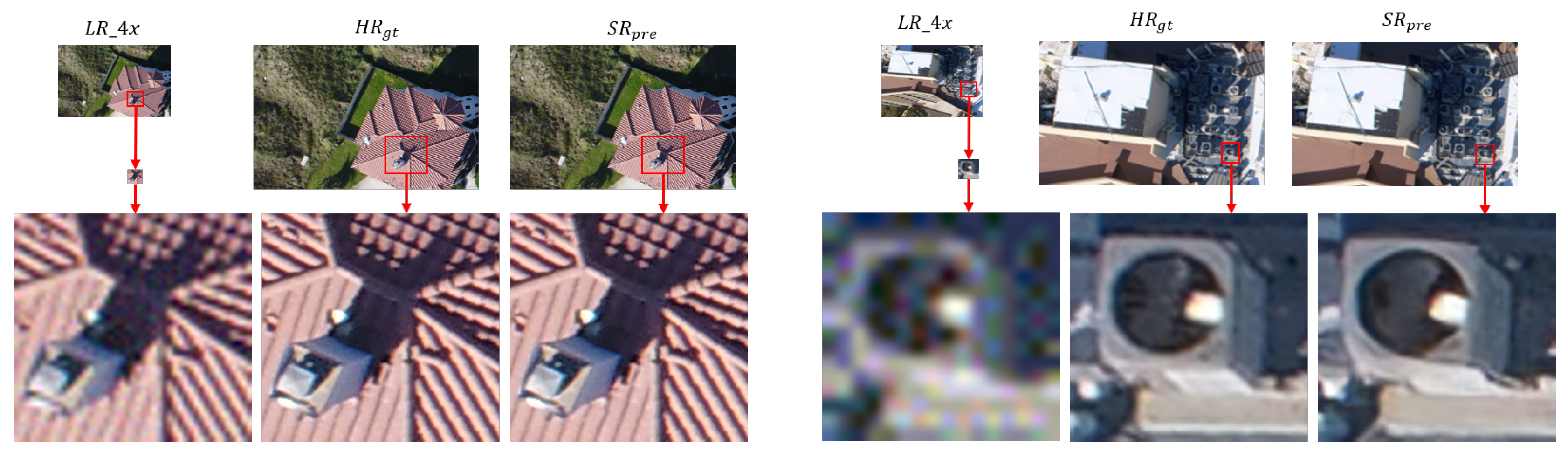
• A high performance DCNN-based SISR model based on GAN architecture [31], known as enhanced SRGAN (ESRGAN) [32], is adopted and trained on a set of LR UAS images virtually generated by downsampling the original HR image set by factor $\times 4$. Additive white Gaussian noise is applied to the LR imagery to make the SISR task more challenging. Such noise can always appear in any digital imaging and image transmission systems due to the electronics, imaging sensor quality, and the interaction of the digital imaging system with the natural environment, such as the level of illumination, temperature, etc [33]. Model performance in recovering the degraded or lost image details and noise reduction in the predicted super-resolved images is then carried out using standard IQMs. In this experiment, IQMs include peak signal-to-noise ratio (PSNR), structure similarity (SSIM) index, and a qualitative analysis through visually inspecting resulting SR images.
• A task-based IQM using Structure-from-Motion (SfM) photogrammetry is carried out on the predicted SR image set.
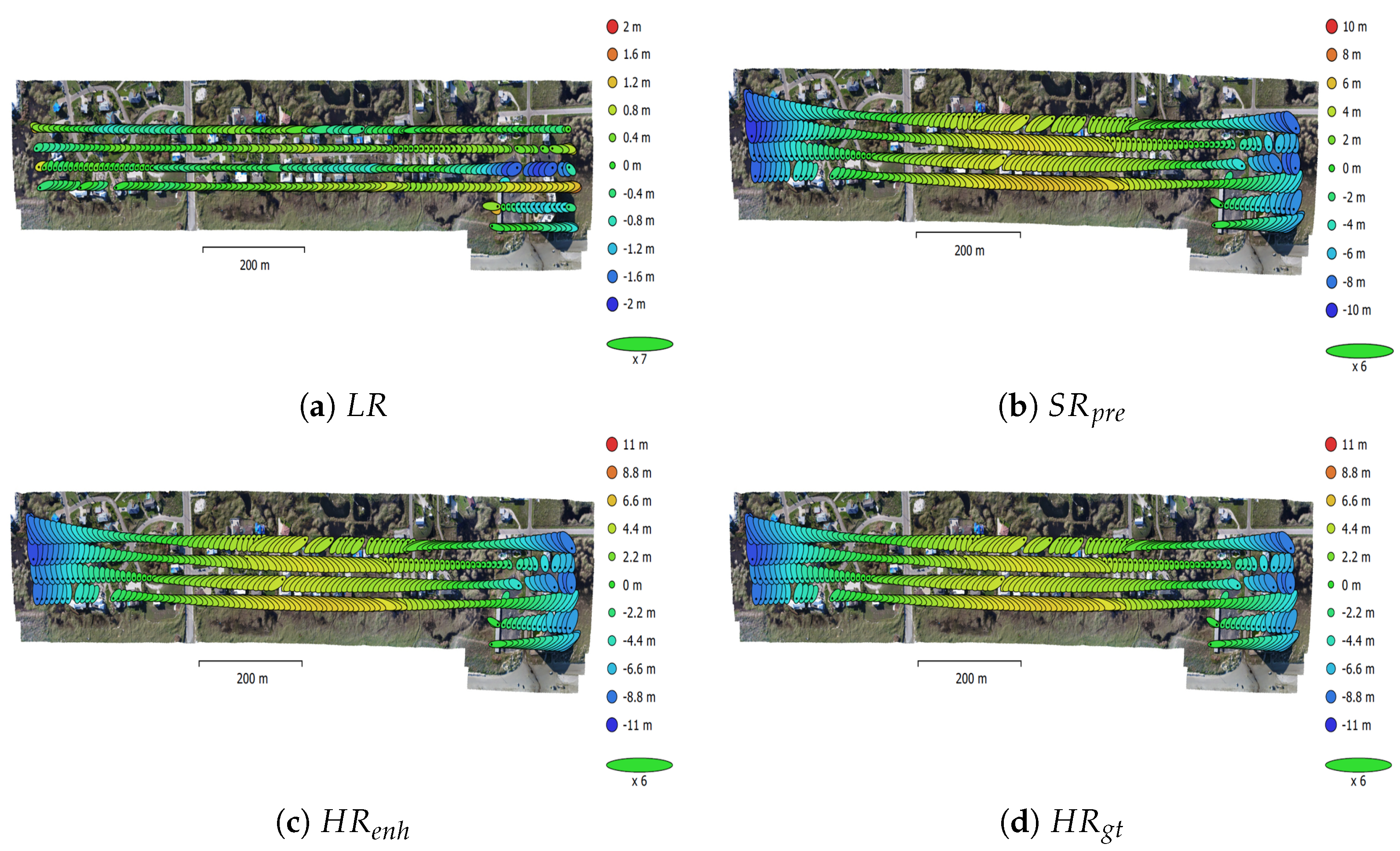
• A comprehensive comparative analysis of SfM derived photogrammetric data products, resulting from processing of the LR, HR, and SR UAS image sets, is carried out. Those products include: the camera calibration and camera pose information, densified 3D point clouds, and digital surface models (DSMs).

In regard to the UAS-SfM task-based evaluation for SR described above, the primary objectives of the experiment are summarized as follows:

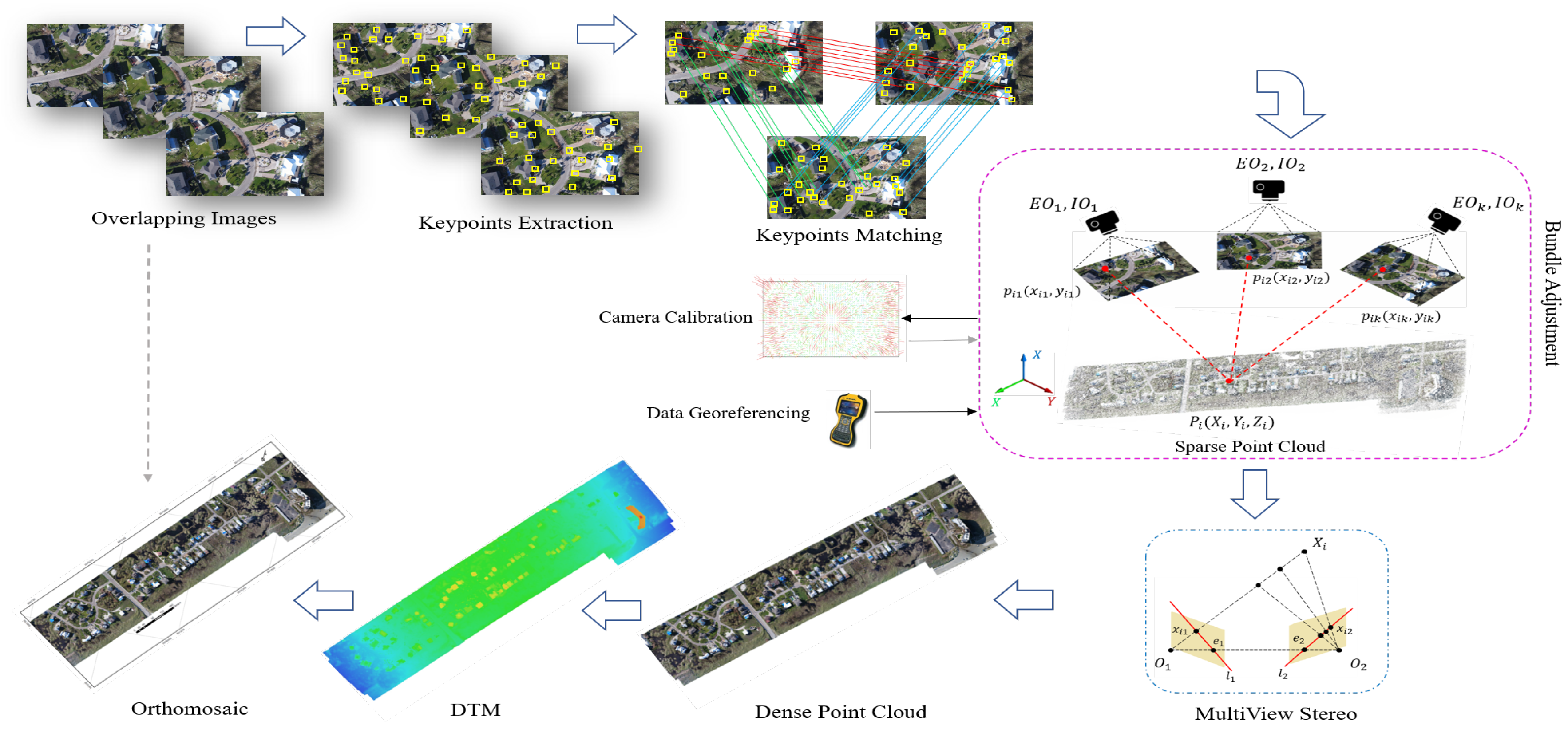
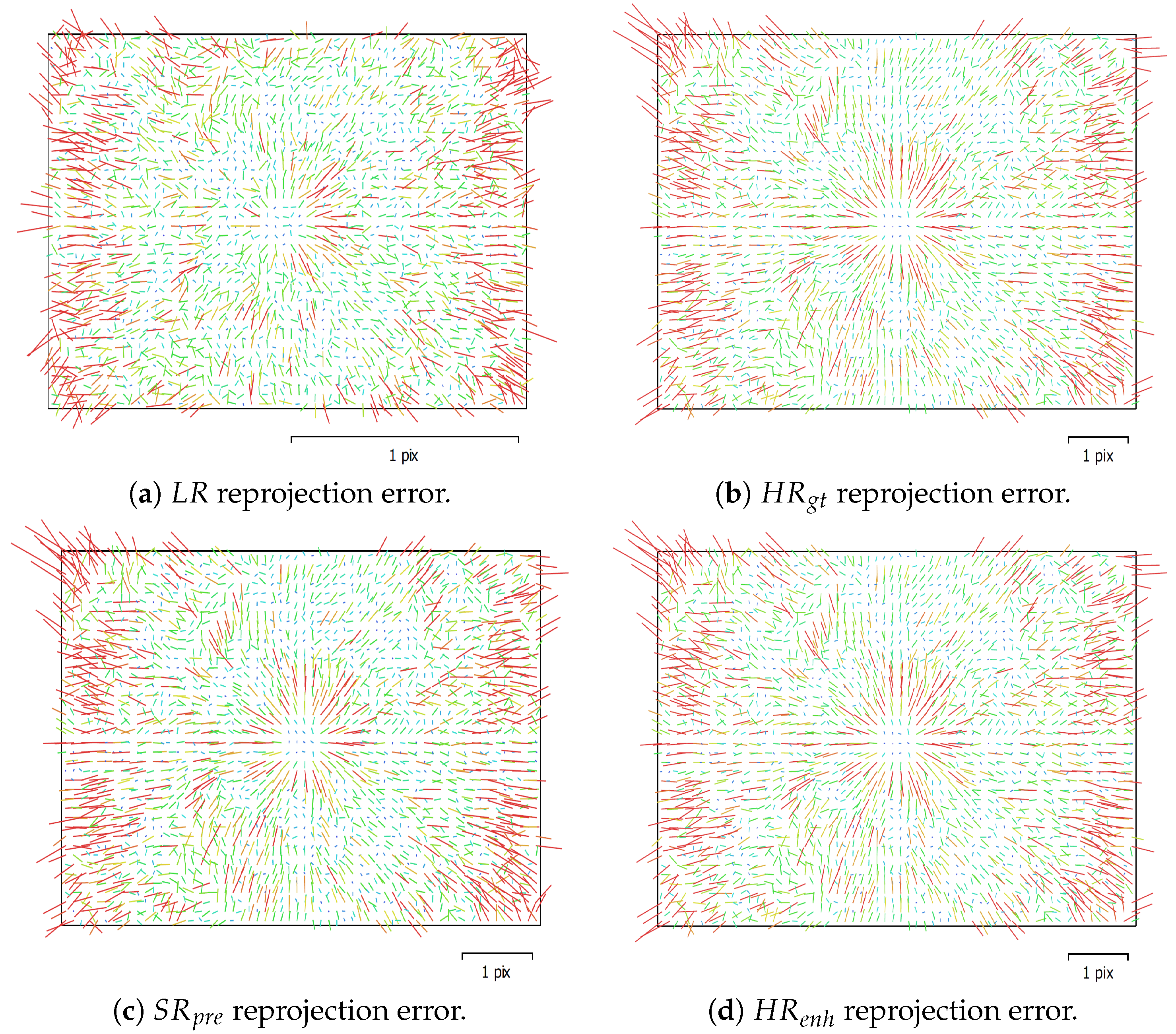
• The performance of the adopted DCNN-based SISR model on retrieving both the interior and exterior geometry of the UAS imagery is investigated. In SfM photogrammetry, the accuracy and reliability of all derived parameters, within the robust bundle adjustment (BA) computations, are closely related to the accuracy and reliability of extracted keypoint features from raw images. Any image distortions and artefacts introduced by adding noise or upsampling images can dramatically affect the reliability of derived parameters within BA computations.
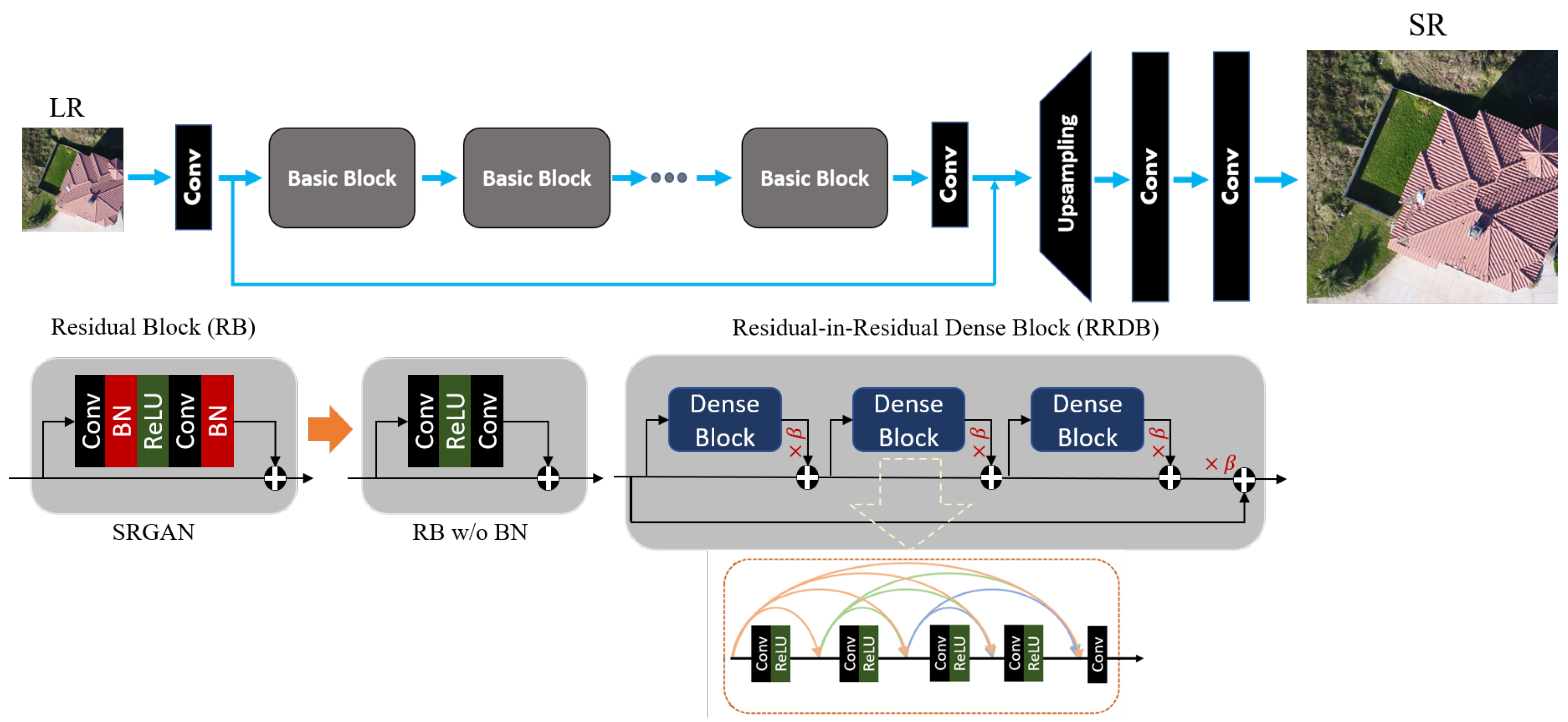
• The potential of the employed DCNN-based SISR model to downgrade the level of inherent and additional noise introduced to the original HR images is investigated. In most image-based 3D reconstruction algorithms, including SfM photogrammetry, lower level of noise in the underlying image set results in estimating the imaging and scene geometry with higher accuracy. That is due to the fact that the feature detection operators, using sophisticated image processing algorithms, extract keypoints features with higher accuracy and lower uncertainty across multiple images in an UAS image set. To do this, the naive pre-trained ESRGAN model, with upscaling factor $\times 1$, is taken as an image restoration network. The idea is to explore the effectiveness of the ESRGAN model, trained on a large number of images within several standard image sets, to downgrade the inherent noise and restore the original UAS HR images.

The remainder of this paper is organized as follows. Section 2 briefly describes image SR as an image upscaling technique to recover the degraded or lost image details in LR images. Section 3 introduces some of the pioneering DCNN-based SISR architectures. GAN-based architecture and its specific cost function for SISR task is later described in Section 3. Learning strategies in Section 4 introduce different cost functions that are usually used in DCNN-based SISR models. Different metrics developed for evaluating the quality of resulting SR images are explained in Section 5. Section 6 explains the experiment including the employed DCNN-based SISR model. Section 7 reports the qualitative and quantitative results showing the performance of ESRGAN model on virtually-generated LR UAS images based on standard IQMs and a task-based IQM using SfM photogrammetry. Section 8 discusses the results in detail. Lastly, Section 9 provides a conclusion and future perspective.

2. Image Super-Resolution

Image SR refers to techniques which aim to restore a HR image from its LR counterpart(s). Their main goal is to recover the high frequency details lost in LR images and remove the degradation caused by the imaging device and/or environment [34,35]. SR is a topic of great interest in digital image processing and many computer vision related applications including HDTV [36], medical imaging [37,38], satellite imaging [39], face recognition [40], security and surveillance [41]. The basic idea in most SR techniques is to extract the non-redundant image content in multiple LR images and combine them to generate a HR image [5]. Single image interpolation is an easy approach within many available SR techniques, which can be used to increase the image size [4]. However, several works showed that it does not provide any additional information and would dramatically decimate details of the image [4,24,42].

Generally, the SR problem assumes the LR image represents a downsampled, noisy, and blurred (by an unknown low-pass filter) version of HR data. Due to the non-invertibility of the degradation process, SR problem is inherently ill-posed [43]. In other words, it is an under-determined inverse problem, of which the solution is not unique. In the typical SR framework, as depicted in Figure 1, the LR image $I_x$ is modeled as follows [44]:

$$I_x=\mathcal{D}(I_y;\delta )$$

(1)

where $I_y$ is the corresponding HR image, $\mathcal{D}$ represents a degradation function, and $\delta$ is a set of parameters, e.g., the parameters of the unknown convolutional kernel, the scaling factor, and some noise related factors, contributing to the degradation process. Under general conditions, the degradation process from $\mathcal{D}$ is unknown and only LR image, $I_x$, is provided. Thus, the SR operation, the reverse path in Figure 1, is an extremely challenging task, which effectively results in a one-to-many mapping from LR to HR image space [25].

Researchers are required to recover the corresponding HR image ${\widehat{I}}_y$ from the LR image $I_x$, so that ${\widehat{I}}_y$ is identical to the ground truth HR image $I_y$, as follows [44]:

$${\widehat{I}}_y=\mathcal{F}(I_x;\theta )$$

(2)

where $\mathcal{F}$ is the super-resolution model and $\theta$ represents the parameters of $\mathcal{F}$. Generally, degradation models combine several operations as follows [44]:

$$\mathcal{D}(I_y;\delta )=(I_y\otimes k){\downarrow }_s+n_{\zeta },\left\{k,s,\zeta \right\}\subset \delta$$

(3)

where $(I_y\otimes k)$ represents the convolution between a blur kernel k and the HR image $I_y$, ${\downarrow }_s$ represents a downsampling process with factor s, and $n_{\zeta }$ is some additive white Gaussian noise with standard deviation $\zeta$.

SR techniques typically assume that high-frequency image contents are redundant and can be reconstructed from low-frequency contents making the SR technique an inference problem [43]. Some SR techniques assume that for reconstructing a HR image of a certain scene, multiple LR instances of the same scene with different perspectives are available. These techniques are categorized as multi-image SR (MISR) approaches [16]. Such methods attempt to invert the downsampling process by exploiting the explicit redundancy and constraining the ill-posed problem with additional information. However, MISR methods are usually computationally expensive because they require complex image registration and fusion in LR image space, where the accuracy of those processes directly affects the quality of the resulting super-resolved images [43]. An alternative approach is single image super-resolution (SISR) [45]. These techniques attempt to exploit the implicit redundancy available in the LR images, in the form of local spatial correlation in an image or additional temporal correlations in a video, and recover lost or deteriorated high-frequency content from a single LR instance. In SISR techniques, prior information is usually required to constrain the solution space [46].

3. Deep Learning for SISR

Learning-based methods, also known as example-based methods [4,47,48,49], aim at estimating an effective mapping from LR to HR image pairs due to their fast computation and superior performance relative to many other traditional techniques [25]. These methods usually exploit machine learning (ML) algorithms to learn the statistical relationships between the HR and corresponding LR images from a substantial number of training samples [25]. Traditional methods for SISR suffer from a few drawbacks [25,43]: (1) unclear and potentially very complex definition of the mapping between the LR and HR image spaces; (2) established sub-optimal high-dimensional mapping; (3) most traditional methods rely upon handcrafted features with expert domain knowledge. Recently, deep learning-based SISR methods have achieved remarkable improvements over all traditional and ML approaches [23,24,25]. These methods take advantage of the huge capacity of DL models to be able to provide an extremely nonlinear mapping in a very high-dimensional space from the input space to the solution space, and efficiently explore that space to find the best solution. These methods usually take a DCNN architecture for low to high-level feature encoding and nonlinear feature mapping.

3.1. DCNN Architectures for SISR

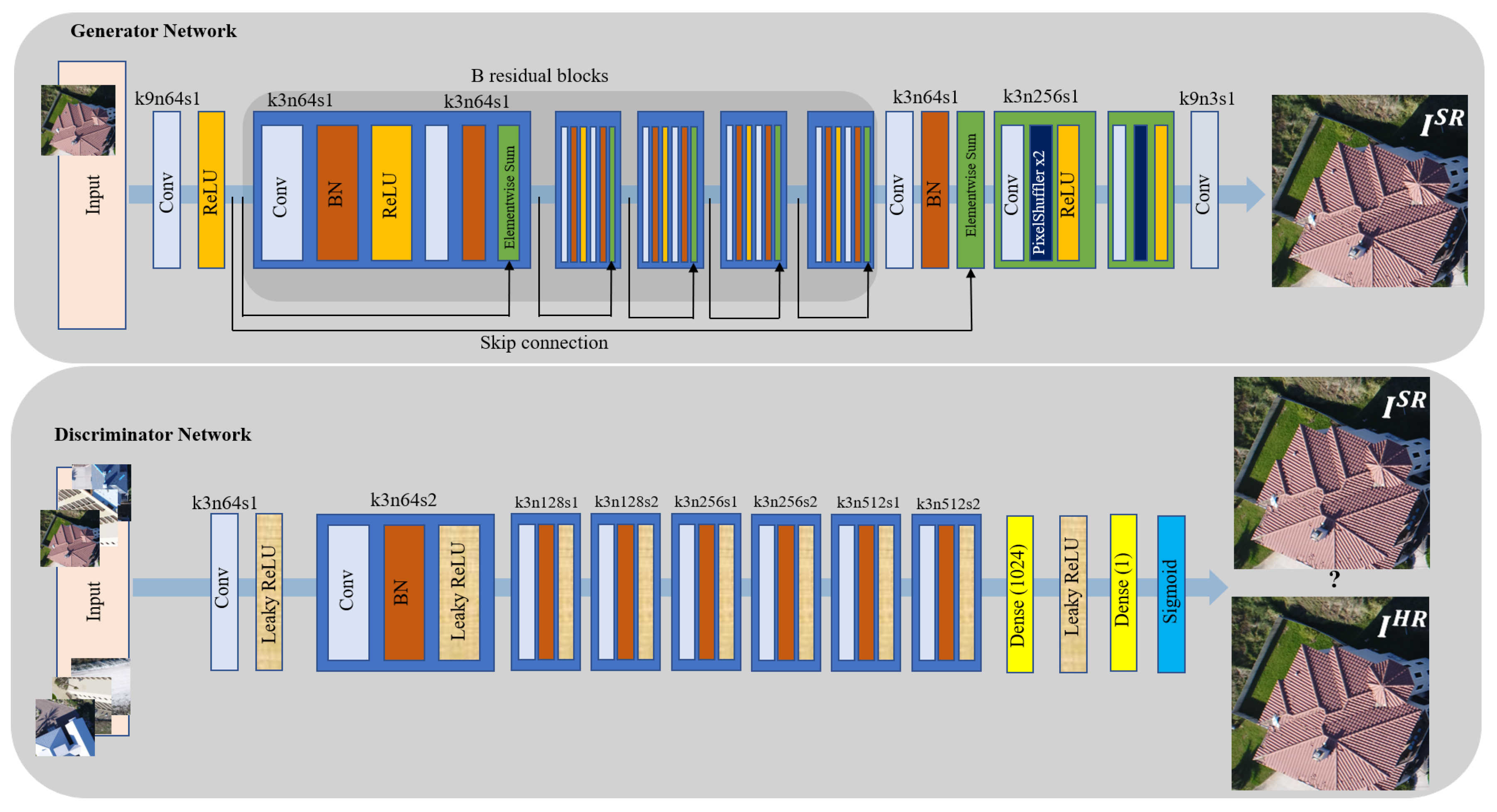
A variety of super-resolution models based on DCNN architectures have been proposed so far. Most of those models focus on supervised super-resolution, requiring both LR images and corresponding HR images, usually as ground truth (GT). These approaches are mostly composed of a set of major components and processing strategies including the model’s main framework, upsampling method, network architecture, and learning strategy.

Super-resolution convolutional neural network (SRCNN) by Dong et al. [24,50] in Figure 2 is a pioneering work in DCNN-based SISR approach. Despite its striking success, SRCNN model suffers from the following issues [25]. (1) Inputs to SRCNN are LR images upsampled to coarse HR images at a desired size using traditional methods (e.g., bicubic interpolation). Introducing interpolated images as inputs to the network have three main drawbacks: (a) severe over-smoothing and noise amplification effects introduced to interpolated inputs can result in further inaccurate estimations of the image content; (b) employing interpolated versions of images, instead of the original LR image, as input is very time-consuming and increases computational complexity almost quadratically [51]; and (c) assuming an unknown kernel in the downsampling process makes adopting a specific interpolated input, as an estimation of the output, unjustified. (2) As mentioned previously, most SR techniques undertake the assumption that the high-frequency content is redundant and can be accurately predicted from the low-frequency data [52]. Thus, exploring more contextual information within large regions of LR images to capture sufficient information for retrieving high-frequency details in predicted HR images seems inevitable. Theoretical work in DL show more contextual information can be achieved by designing very deep architectures with larger receptive fields, which can result in expanding the final solution space [19,53,54,55,56]. In some situations, effectively attaining more hierarchical representations can be achieved by increasing the DL network depth [53]. In recent years, many different CNN-based architectures have been developed, which exploit a very deep and sophisticated architecture, including residual and/or dense feature mapping [19,56], to solve complex problems more efficiently [25,44].

3.2. GAN for SISR

Introduction of recent innovative and deeper CNN-based architectures for SISR has already led to breakthroughs in accuracy and speed. Photo-realistic SISR GAN (SRGAN) [23], illustrated in Figure 3, was introduced for recovering the finer texture details when resolving at large upscaling factors. Those recovered fine details in SR images not only make predicted HR images more appealing to a human, but also have a great impact on the accuracy and reliability of imaging geometry and scene details when they are retrieved by the SfM phtotogrammetry process.

The basic SRGAN model is built upon the residual blocks [19] and trained under the perceptual loss in a GAN framework, which makes it capable of predicting photo-realistic images for $\times 4$ upscaling factor [23]. The SRGAN model has shown significant improvement on overall visual quality of SR images over all previously introduced PSNR-oriented methods [23,32].

GAN [31] introduced by Goodfellow et al. tries to solve the adversarial min-max problem [23]:

$$\begin{array}{cc}\hfill \underset{{\theta }_G}{\min }\underset{{\theta }_D}{\max }& {\mathbb{E}}_{I^{HR}\sim p_{train}(I^{HR})}\left[log{D}_{{\theta }_D}(I^{HR})\right]+\hfill \\ \hfill & {\mathbb{E}}_{I^{LR}\sim p_G(I^{LR})}\left[log(1-D_{{\theta }_D}\left(G_{{\theta }_G}(I^{LR})\right)\right]\hfill \end{array}$$

(4)

where it allows the network to train a generative model G with the purpose of fooling a discriminator D that is simultaneously trained to discriminate the SR images from the original HR images.

The formulated perceptual loss consists of a weighted sum of a content loss (${\mathcal{L}}_X^{SR}$) and an adversarial loss component (${\mathcal{L}}_{Gen}^{SR}$) as follows [23]:

$${\mathcal{L}}^{SR}=\underset{\mathrm{perceptual}\mathrm{loss}}{\underbrace{\underset{\mathrm{content}\mathrm{loss}}{\underbrace{{\mathcal{L}}_X^{SR}}}+\underset{\mathrm{adversarial}\mathrm{loss}}{\underbrace{{10}^{-3}{\mathcal{L}}_{Gen}^{SR}}}}}$$

(5)

Content loss motivated by perceptual similarity chooses the solution based on the perceptual similarity from the high dimensional solution space [23]. Instead of relying on pixel-wise losses, Ledig et al. define VGG loss based on ReLU activation layers and 19 layers VGG network [53], where VGG loss is computed as the Euclidean distance between the feature representations of a reconstructed image $G_{{\theta }_G}(I^{LR})$ and the ground truth image $I^{HR}$ as follows [23]:

$${\mathcal{L}}_{VGG/i,j}^{SR}=\frac{1}{W_{i,j}{H}_{i,j}}\sum _{x=1}^{W_{i,j}}\sum _{y=1}^{H_{i,j}}{\left({\varphi }_{i,j}{(I^{HR})}_{x,y}-{\varphi }_{i,j}{(G_{{\theta }_G}(I^{LR}))}_{x,y}\right)}^2$$

(6)

where ${\varphi }_{i,j}$ represents the feature map obtained by the j-th convolution (after activation) before the i-th maxpooling layer within the VGG-19 network. $W_{i,j}$ and $H_{i,j}$ describe the dimensions of the respective feature maps within the VGG network.

Adversarial loss, which is the generative component of SRGAN to the perceptual loss, encourages the network to favor solutions residing on the natural image manifold [23]. The generative loss (${\mathcal{L}}_{Gen}^{SR}$) is evaluated, in a probabilistic framework, based on the performance of the discriminator $D_{{\theta }_D}(.)$ over a training sample set as [23]:

$${\mathcal{L}}_{Gen}^{SR}=\sum _{n=1}^N-log{D}_{{\theta }_D}(G_{{\theta }_G}(I^{LR}))$$

(7)

where, $D_{{\theta }_D}(G_{{\theta }_G}(I^{LR}))$ represents the probability that the generated image $G_{{\theta }_G}(I^{LR})$ is a natural HR image. As a consequence of exploiting adversarial loss, the discriminator network is trained to push SISR solutions to the natural image manifold.

4. Learning Strategies

Learning the end-to-end mapping function $\mathcal{F}$ to map a LR image $I^{LR}$ to the corresponding reconstructed SR image $I^{SR}={\widehat{I}}^{HR}$, which is an approximation of the real HR image $I^{HR}$, requires the estimation of network parameters $\theta$. This is attained via minimizing the loss between the super-resolved images $I^{SR}=\mathcal{F}\left(I^{LR};\theta \right)$ and the corresponding HR images $I^{HR}$. In this section, different loss functions that are widely used in SISR techniques are introduced. For the sake of brevity, the subscript y is dropped from the ground truth (target) HR image $I_y$ and the reconstructed HR image ${\widehat{I}}_y$ in the rest of this section.

4.1. Pixel Loss

Pixel loss evaluates the pixel-wise difference between two images, mainly in the form of $L_1$ distance, i.e., mean absolute error (MAE), or $L_2$ distance, i.e., mean square error (MSE). In so doing, it attempts to capture and solve the inherent uncertainty in retrieving lost high-frequency components by minimizing related loss functions as follows [44]:

$${\mathcal{L}}_{pixel-L_1}\left(I^{HR},I^{SR}\right)=\frac{1}{hwc}\sum _{i,j,k}|I_{i,j,k}^{HR}-I_{i,j,k}^{SR}|$$

(8)

$${\mathcal{L}}_{pixel-L_2}\left(I^{HR},I^{SR}\right)=\frac{1}{hwc}\sum _{i,j,k}{\left(I_{i,j,k}^{HR}-I_{i,j,k}^{SR}\right)}^2$$

(9)

where h, w and c are the height, width and number of channels of the reconstructed images, respectively. Charbonnier loss [57,58], is a variant of $L_1$ loss, given by [44]:

$${\mathcal{L}}_{pixel-Cha}\left(I^{HR},I^{SR}\right)=\frac{1}{hwc}\sum _{i,j,k}\sqrt{{\left(I_{i,j,k}^{HR}-I_{i,j,k}^{SR}\right)}^2+{ϵ}^2}$$

(10)

where $ϵ$ is a small constant (e.g., $1e-3$) for numerical stability.

The pixel loss constraint results in a super-resolved image $I^{SR}$, which is close to the ground truth HR image $I^{HR}$ in the pixel values. In comparison with $L_2$ loss, the $L_1$ loss shows higher performance and better convergence [44,59]. Using pixel loss as the loss function favors a high peak signal-to-noise ratio (PSNR). According to its definition, PSNR is heavily correlated with pixel-wise deviation, where minimizing pixel loss directly maximizes PSNR [23]. Moreover, it is partially related to the image perceptual quality. Thus, pixel loss has become the most widely used loss function in SR field.

Minimizing the pixel loss encourages finding plausible solutions, based on pixel-wise average, in the high dimensional solution space. In return, such solutions can be overly-smooth with poor perceptual quality [23,60,61]. Thus, in order to capture the reconstruction error and image quality more efficiently, a variety of other loss functions, such as content loss [61] and adversarial loss [23], were introduced to the SR field.

4.2. Perceptual/Content Loss

To evaluate image quality based on perceptual similarity, perceptual-driven approaches have also been proposed [62,63]. More convincing results from the image perceptual point of view, for both SR and artistic style-transfer tasks, are offered in this category [23,63,64]. By minimizing the error in the feature space instead of the pixel space, perceptual loss or content loss, attempts to improve the image visual quality. Denoting feature maps computed within the l-th layer of the network as ${\varphi }^{(l)}(.)$, the content loss is evaluated using the Euclidean distance between corresponding feature maps from the original and super-resolved images as follows [44]:

$${\mathcal{L}}_{content}\left(I^{HR},I^{SR};\varphi ,l\right)=\frac{1}{h_l{w}_l{c}_l}\sum _{i,j,k}\sqrt{{\left({\varphi }_{i,j,k}^{(l)}\left(I^{HR}\right)-{\varphi }_{i,j,k}^{(l)}\left(I^{SR}\right)\right)}^2}$$

(11)

where $h_l$, $w_l$ and $c_l$ represent the height, width and number of channels of the extracted feature maps in layer l, respectively.

Content loss encourages transferring the learned knowledge of hierarchical image features from a pre-trained classification network, usually VGG or ResNet, to the SR task [12,23,32,65].

4.3. Adversarial Loss

Adversarial learning [31] is adopted for SR task in a straightforward way, in which SR model is considered as a generator, and a discriminator network is added to the model to discriminate the generated image $I^{SR}$ from the real image $I^{HR}$. Adversarial loss for SRGAN [23] is as follows [44]:

$${\mathcal{L}}_{gan\_G}\left(I^{LR};D_{{\theta }_G}\right)=-log{D}_{{\theta }_D}\left(G_{{\theta }_G}(I^{LR})\right),$$

(12)

$${\mathcal{L}}_{gan\_D}\left(I^{HR},I^{SR};D_{{\theta }_D}\right)=-log{D}_{{\theta }_D}\left(I^{HR}\right)-log{D}_{{\theta }_D}\left(I^{SR}\right)$$

(13)

where ${\mathcal{L}}_{gan\_G}$ and ${\mathcal{L}}_{gan\_D}$ denote the adversarial loss of the generator $G_{{\theta }_G}$, which is the SR model, and the discriminator $D_{{\theta }_D}$, which is a deep CNN model for binary classification, respectively. ${\theta }_G$ and ${\theta }_D$ are the parameters of the generator and discriminator, and $I^{SR}=G_{{\theta }_G}(I^{LR})$ is the generated image approximating the corresponding ground truth HR image.

In practice, some researchers employ a combination of multiple loss functions in their DCNN-based SISR architectures for more efficient learning and to better constrain different aspects of SR image reconstruction [12,23,57,66,67]. However, how to efficiently combine multiple loss functions with effective weights emphasizing their contribution in the learning process, remains an active area of SR research.

5. Image Quality Metrics

Image quality metrics, usually referred to as image quality measures (IQMs), are measures focusing on significant visual attributes of images where they attempt to quantify the perceptual assessments of an image when it is evaluated in a certain image quality assessment (IQA) approach [60]. IQA approaches are categorized into subjective methods, which focus on quantifying human perception, and objective methods, which are based on some computational models [60]. The subjective methods can be more accurate but they are usually inconvenient, time-consuming, and expensive to implement [60]. As a result, objective methods are currently considered the mainstream among IQMs. Since the objective methods cannot efficiently capture the human visual perception, the metrics evaluated under these methods may show some inconsistency with those from subjective methods [60].

Objective IQA methods are divided into three types [60] including: (1) full-reference methods requiring corresponding images with perfect or high quality image content; (2) reduced-reference methods, which apply IQMs on the extracted features from both images and their corresponding high quality counterparts; (3) no-reference methods, which try to evaluate image quality in a blind way without any reference images. In supervised SISR, high quality HR images are usually available for evaluating different IQMs. This section introduces some of the most commonly used IQMs, covering both subjective IQA methods and objective IQA methods.

5.1. Peak Signal-to-Noise Ratio (PSNR)

PSNR measure refers to the ratio between a signal’s maximum power and the power of the signal’s noise, which affects the quality of the signal’s representation. Due to the very wide dynamic range (i.e., ratio of highest and lowest values) of most signals, the PSNR is usually expressed in the logarithmic decibel scale. PSNR is used to measure the reconstruction quality of lossy transformations including image compression and inpainting. For image SR task, PSNR is defined using the maximum possible pixel value in the underlying image, and the mean squared error (MSE) between two corresponding images. Given the high quality image I and the corresponding reconstructed (super-resolved) image $\widehat{I}$, both of which include N pixels, the MSE and the PSNR measures are defined as follows [25]:

$$MSE=\frac{1}{N}\sum _{i=1}^N{\left(I_i-{\widehat{I}}_i\right)}^2$$

(14)

$$PSNR=10{log}_{10}\left(\frac{L^2}{MSE}\right)$$

(15)

L denotes the maximum possible pixel value in the image. For 8-bit image representations, for example, L equals to 255 and the typical values for the PSNR may vary from 20 to 40 dB, where the higher the PSNR value, the better the quality of the reconstructed image as it tries to minimize MSE between the images with respect to the maximum pixel value of the input image. When L is fixed, PSNR is only related to the pixel-wise distances between two images represented by MSE. The ability of MSE, and consequently PSNR, to capture perceptually relevant differences, such as high texture detail, is very limited meaning that PSNR does not care about human visual perception and photo-realistic characteristics of the image. This often leads to poor performance of PSNR when used to assess the quality of super-resolved images in natural scenes. However, due to the lack of an efficient and comprehensive IQM that considers image quality from all perspectives, PSNR remains the most widely used metric for evaluating image quality in SR tasks.

5.2. Structural Similarity (SSIM) Index

Similar to the human visual system, which is highly adapted for extracting structural information from the viewing scene, SSIM index provides a perceptual metric that quantifies image quality degradation based on perceived image quality [68]. Made up of three relatively independent terms, luminance, contrast, and structure, SSIM index estimates the visual impact of those factors when they are modified in the reconstructed image. Those modifications may comprise shifts in image luminance, alterations in image contrast, and any other remaining deviations collectively identified as structural changes [60].

For an original high quality image I and its reconstructed counterpart $\widehat{I}$, the SSIM index is defined as follows [69]:

$$SSIM\left(I,\widehat{I}\right)={\left[C_l(I,\widehat{I})\right]}^{\alpha }{\left[C_c(I,\widehat{I})\right]}^{\beta }{\left[C_s(I,\widehat{I})\right]}^{\gamma }$$

(16)

where $\alpha >0$, $\beta >0$, and $\gamma >0$ control the relative significance of each of the three terms of the index. In some implementations, $\alpha =\beta =\gamma =1$ [60]. The luminance, $C_l$, contrast, $C_c$, and structural, $C_s$, components of the SSIM index are defined as follows [69]:

$$C_l\left(I,\widehat{I}\right)=\frac{2{\mu }_I{\mu }_{\widehat{I}}+C_1}{{\mu }_I^2+{\mu }_{\widehat{I}}^2+C_1}$$

(17)

$$C_c\left(I,\widehat{I}\right)=\frac{2{\sigma }_I{\sigma }_{\widehat{I}}+C_2}{{\sigma }_I^2+{\sigma }_{\widehat{I}}^2+C_2}$$

(18)

$$C_s\left(I,\widehat{I}\right)=\frac{{\sigma }_{I\widehat{I}}+C_3}{{\sigma }_I{\sigma }_{\widehat{I}}+C_3}$$

(19)

where ${\mu }_I,{\sigma }_I$ and ${\mu }_{\widehat{I}},{\sigma }_{\widehat{I}}$ represent the means and standard deviations of the original high quality image and the corresponding reconstructed image, respectively, and ${\sigma }_{I\widehat{I}}$ is the covariance of the two images. The constants $C_1$, $C_2$, and $C_3$ in Equations (17)–(19) help to avoid instability when the denominators are close to zero. The formulation given in Equation (16) guarantees symmetry, where $SSIM(I,\widehat{I})=SSIM(\widehat{I},I)$. Moreover, the index ensures a bounded $SSIM(I,\widehat{I})\le 1$. Furthermore, there is a unique maximum, where $SSIM(I,\widehat{I})=1$ if and only if $I=\widehat{I}$. For an 8-bit grayscale image containing $L=2^8=256$ gray-levels, $C_1={(k_1.L)}^2$, $C_2={(k_2.L)}^2$, and $C_3=C_2/2$, where $k_1\ll 1$ and $k_2\ll 1$ are very small constants for avoiding instability. According to the above formulas, SSIM can be represented as follows [69]:

$$SSIM\left(I,\widehat{I}\right)=\frac{\left(2{\mu }_I{\mu }_{\widehat{I}}+C_1\right)\left({\sigma }_{I\widehat{I}}+C_2\right)}{\left({\mu }_I^2+{\mu }_{\widehat{I}}^2+C_1\right)\left({\sigma }_I^2+{\sigma }_{\widehat{I}}^2+C_1\right)}$$

(20)

In addition, to deal with uneven distribution of image statistical features or distortions, it is more reliable to perform image quality assessment locally rather than globally. Thus, mean structural similarity (mSSIM) [60] is proposed for locally assessing SSIM. This technique splits the images into multiple windows in which the SSIM of each window is evaluated, and finally averages it over all windows across the image. Because it evaluates the image reconstruction quality from the perspective of the human visual system, SSIM index better meets the requirements of perceptual assessment. The efficiency of SSIM-based IQM outperforms those based on MSE and the related PSNR over natural images including a wide variety of image distortions [69]. Those properties make SSIM index a widely used IQM among others in most SR tasks [70,71]. However, in some cases, SSIM index may lead to similar results in evaluation of image performance with PSNR metric [60].

5.3. Task-Based Evaluation

Evaluating image reconstruction performance via other image analysis tasks is also an effective IQM [11,12,13,72]. Specifically, this technique feeds the original high quality image and the corresponding reconstructed image into a trained model for a specific vision task, and evaluates the reconstruction quality by comparing the relative impact of reconstructed images on the prediction performance with respect to that from high quality original HR images. The vision tasks used for this evaluation technique include face recognition [73,74], face alignment and parsing [65,75], and object recognition [12,76]. However, certain vision tasks may focus on some specific image attributes that are more favorable to the task, and may not be aware or care about the visual perceptual quality of the image. For example, most object recognition models mainly focus on the high-level semantics while ignoring the image contrast and noise. But on the other hand, in some domain-specific applications, such as super-resolving surveillance video for face recognition, task-based IQM may reflect the performance of the SR models.

6. Methods and Materials

6.1. Methodology

In this SISR experiment, enhanced SRGAN (ESRGAN) [32] model is employed which improves the original SRGAN model in three aspects. First, ESRGAN improves the network by designing a Residual-in-Residual Dense Block (RRDB), illustrated in Figure 4, which offers higher capacity and easier training. Second, the Relativistic average GAN (RaGAN) [77], which learns to distinguish a more realistic image from a corresponding less realistic image, replaces the original discriminator in SRGAN, which simply judges whether an image is real or fake. According to [77], this improvement allows the ESRGAN generator to recover more realistic texture details. Third, ESRGAN adjusts the perceptual loss in the original SRGAN model by using VGG features before activation, rather than features after activation. This empirically leads to sharper edges and more visually pleasing results. Some properties of ESRGAN model is discussed below in more details.

Network Architecture: ESRGAN employs the basic architecture of SRResNet [23] for feature learning in the LR feature space. ESRGAN introduces two modifications to the generator architecture of SRGAN to improve the quality of the super-resolved images, G: (1) it removes all batch normalization (BN) layers; (2) it replaces the original basic residual block (RB) in SRGAN with a more compact RRDB architecture. According to Figure 4, by optimally combining multi-level residual blocks, the RRDB design improves the perceptual quality of super-resolved images [32]. When the statistics of image batches for training and testing are significantly high, BN layers tend to introduce unpleasant artefacts limiting the generalization ability [32]. Removing BN layers, especially under the GAN framework which is more prone to artefact generation, leads to consistent higher performance, lower computational complexity, and better generalization in the network [32,59]. In addition to the architectural improvement, to facilitate training a very deep network, ESRGAN exploits residual scaling technique [55,59] to prevent instability in training by scaling down the residuals using a scaling factor between 0 and 1 before adding them to the main path. Moreover, ESRGAN employs a smarter initialization technique, which has empirically been shown to provide easier training when the initial parameter variance becomes smaller [32].

Relativistic Discriminator: The original SRGAN model uses the standard discriminator expressed as $D(I)=\sigma (C(I))$, where $\sigma$ is the sigmoid function and $C(I)$ is the discriminator output. This definition estimates the probability that the input image I is the original HR (real) image or the super-resolved (fake) image. In contrast, a relativistic discriminator predicts the probability that the original HR image $I^{HR}$ is relatively more realistic than the super-resolved image $I^{LR}$ as shown in Figure 5. The Relativistic average Discriminator (RaD) [77] is formulated as: $D_{Ra}(x_r,x_f)=\sigma \left(C(x_r)-{\mathbb{E}}_{x_f}\left[C(x_f)\right]\right)$, where $D_{Ra}$ is RaD function and $x_r$ and $x_f$ are the real (original HR) and fake (super-resolved) images, respectively. ${\mathbb{E}}_{x_f}[.]$ represents average over all generated or fake images in each individual mini-batch. The discriminator loss, ${\mathcal{L}}_D^{Ra}$, is defined as follows [32].

$${\mathcal{L}}_D^{Ra}=-{\mathbb{E}}_{I^{HR}}\left[log\left(D_{Ra}(I^{HR},I^{SR})\right)\right]-{\mathbb{E}}_{I^{SR}}\left[log\left(1-D_{Ra}(I^{SR},I^{HR})\right)\right]$$

(21)

The adversarial loss for generator, ${\mathcal{L}}_G^{Ra}$, is in a symmetrical form as [32]:

$${\mathcal{L}}_G^{Ra}=-{\mathbb{E}}_{I^{HR}}\left[log\left(1-D_{Ra}(I^{HR},I^{SR})\right)\right]-{\mathbb{E}}_{I^{SR}}\left[log\left(D_{Ra}(I^{SR},I^{HR})\right)\right]$$

(22)

where $I^{LR}$ and $I^{SR}=G(I^{LR})$ stand for the input LR image and the predicted super-resolved image, respectively. In contrast to the adversarial loss for the generator in the original SRGAN model, ${\mathcal{L}}_{Gen}^{Ra}$ in Equation (7), in which only gradients from the generated images take part in adversarial training, the adversarial loss for the generator in ESRGAN, ${\mathcal{L}}_G^{Ra}$ in Equation (22), contains both $I^{SR}$ and $I^{HR}$. This property causes the gradients from both real images and generated images to participate in adversarial training [32].

Perceptual Loss: ESRGAN suggests a more effective perceptual loss ${\mathcal{L}}_{percep}$ by computing distances between corresponding feature maps before activation rather than after activation, as practiced in the original SRGAN model. Employing features before the activation layers overcomes two drawbacks in the original design including extreme sparsity in the activated feature maps, and inconsistent brightness reconstruction compared with the original HR image. Specially within a very deep network, sparsity within feature maps leads to weak supervision and inferior performance. The loss function for the generator in ESRGAN model is as follows [32]:

$${\mathcal{L}}_G={\mathcal{L}}_{percep}+\lambda {\mathcal{L}}_G^{Ra}+\eta {\mathcal{L}}_1$$

(23)

where ${\mathcal{L}}_1={\mathbb{E}}_{I^{LR}}{\parallel G(I^{LR})-I^{HR}\parallel }_1$ is the content loss that evaluates the $L_1$ distance between super-resolved image $G(I^{LR})$ and the original HR image $I^{HR}$, and $\lambda$ and $\eta$ are coefficients to balance different loss terms.

6.2. IQMs for SR Images

In this experiment, a comprehensive quantitative and qualitative assessment is performed on the resulting SR images by exploiting some standard IQMs that are frequently used for assessing the performance of different SISR models. Furthermore, a task-based IQM based on the SfM photogrammetry [78] procedure is carried out. Applying any type of image processing algorithm on a raw aerial image set can dramatically affect the precision and accuracy of retrieving the interior and exterior geometry of a camera at image acquisition time. That, consequently, may lead to a significant decrease in the quality and final accuracy of the main SfM photogrammetry products, such as point clouds, DSMs, and orthoimages. The authors believe that the chosen task-based IQM can more accurately exhibit the effectiveness and performance of DCNN-based SISR to enhance the spatial resolution of LR imagery in RS applications. More specifically, where highly accurate spatial products from processing RS images are required.

6.2.1. Standard IQM methods

PSNR and SSIM index are evaluated as standard IQMs for quantitative assessment of predicted SR images. Choosing those two IQMs enables performance comparison in DCNN-based SISR applications when it is applied on two different categories of images (general images and aerial RS images).

6.2.2. SfM Photogrammetry for Task-Based IQM

SfM photogrammetry procedure, as illustrated in Figure 6, is employed on all available image sets including HR ground truth, LR, and predicted SR image sets. SfM photogrammetry is a low-cost method, based on stereoscopic photogrammetry, for highly accurate topographic reconstruction using a series of overlapping images acquired from multiple viewpoints [78]. In contrast to traditional photogrammetry, in SfM photogrammetry, interior geometry of the camera, usually referred to as interior orientation ($IO$) parameters, position and orientation of each camera station with respect to the scene’s global coordinate system, commonly called exterior orientation ($EO$) parameters, and the geometry of the scene, i.e., the 3D coordinate of each point of the 3D scene, are resolved automatically. All required parameters are calculated simultaneously based on the highly redundant and iterative bundle adjustment (BA) computations using a rich database of corresponding image features automatically extracted from a set of multiple overlapping images [79]. SfM photogrammetry addresses the key problem of determining the 3D locations of a large number of corresponding features extracted from multiple overlapping images, taken from different positions and angles with respect to the 3D scene.

Most image-based 3D reconstruction software that work based on the SfM photogrammetry principle, first solve for camera $IO$ and $EO$ parameters followed by a multi-view stereo (MVS) algorithm to escalate the density of the sparse point cloud generated by the SfM algorithm [78]. In the first step, several overlapping images are imported into the software, and a keypoints detection algorithm, usually the popular scale invariant feature transform (SIFT) algorithm [80], is applied to detect keypoints and keypoint correspondences across and between all images using a keypoint descriptor. In the SIFT algorithm, for example, the keypoint descriptor is determined by computing local image gradients and transforming them into a representation substantially insensitive to some image feature variations, including illumination, orientation, and scale [80]. These descriptors are unique enough to allow features to be matched in large image datasets. The BA technique is performed to minimize the errors in the phase of finding point correspondences [78].

In addition to solving for $IO$ and $EO$ parameters, which indicate camera calibration and pose parameters, respectively, the SfM algorithm generates a sparse point cloud using the image coordinates of all corresponding keypoints, $IO$, and $EO$ parameters of the camera in all imaging stations. The coordinate system related to the generated point cloud is arbitrary. In order to transform the point cloud coordinate system to any local or global coordinate system, a georeferencing phase should be adopted. In that phase, a few ground control points (GCPs) with known 3D coordinates in a local or global coordinate reference frame using land surveying or initial camera positions, e.g., using global navigation satellite system (GNSS), is typically required. In this experiment, it is not necessary to perform the georeferencing step since all images are processed in the same reference frame. The $IO$ and $EO$ parameters for each camera are used as the input to the MVS algorithm. Leveraging the known $IO$ and $EO$ parameters for each individual camera, MVS initiates an intense search algorithm to find more correspondences along all existing epipolar lines in all overlapping images. The accuracy of the MVS algorithm and the quality of the dense point cloud generated by the MVS algorithm is highly dependent on the reliability of the $IO$ and $EO$ parameters calculated from the initial BA computations [81].

Images captured at high spatial resolutions, in general, return the most keypoints and keypoints correspondences in overlapping images. In addition to the major contribution of the natural texture in the $3D$ scene, the quality of the generated point cloud highly depends on several other factors including the density, sharpness, contrast, and resolution of the image content within the image set [78]. Moreover, decreasing the image acquisition distance, or flight height above ground, leads to an increase in the image spatial resolution or a finer GSD. This will further enhance the spatial density and spatial resolution of the resulting point cloud [78]. However, the uncertainty in keypoints extraction and matching, which is a typical issue in all low quality LR images, may result in poor estimation of a camera’s $IO$ and $EO$ parameters leading to a very inaccurate and erroneous 3D point cloud.

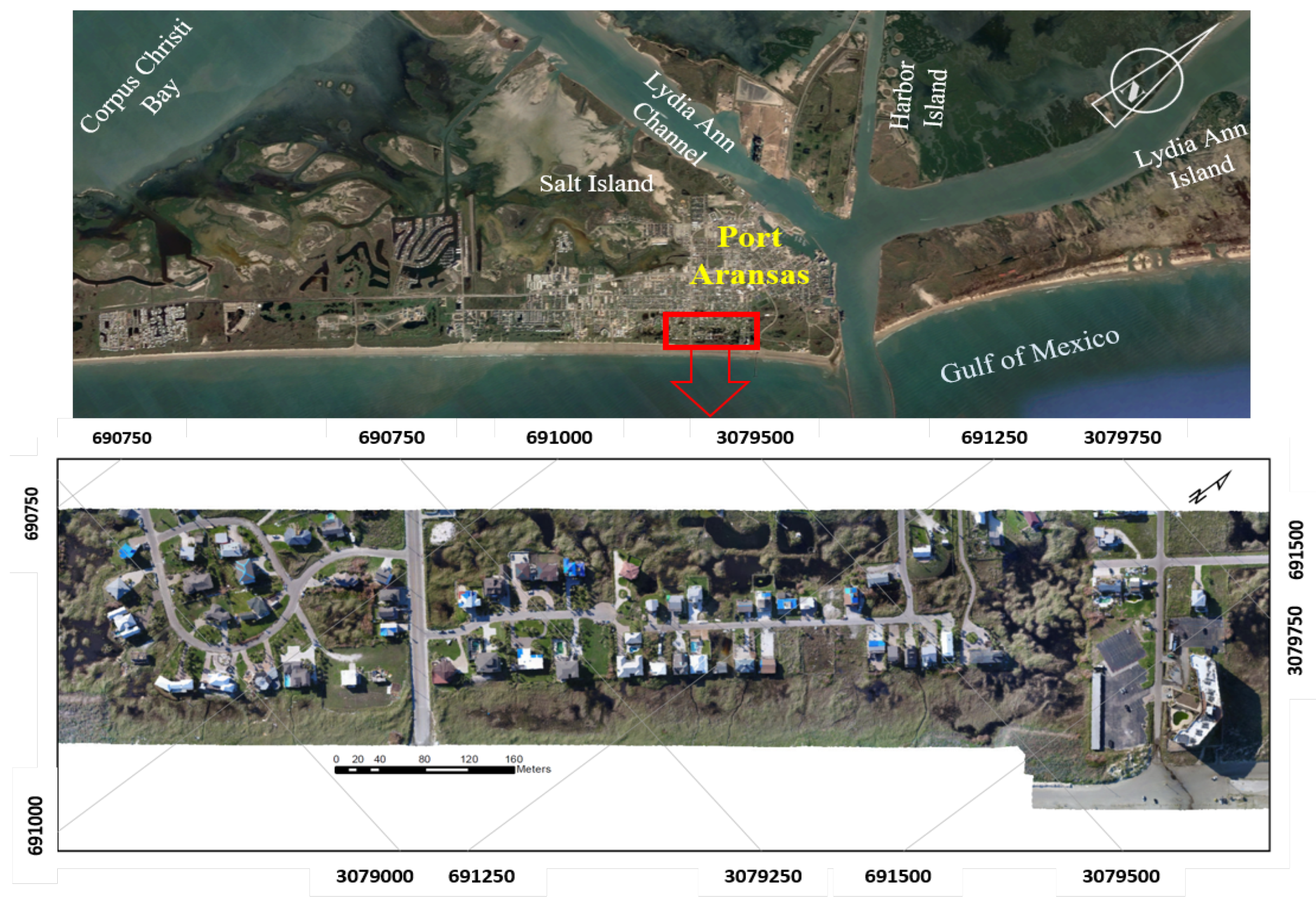
6.3. Study Site and Dataset

Port Aransas is a town located on Mustang Island along the southern Texas Gulf of Mexico coastline, USA Figure 7. In 2017, Hurricane Harvey, a category 4 hurricane, made landfall to the north of Port Aransas along San Jose Island on the night of 25 August 2017. The southern portion of the eye wall passed within close proximity to Port Aransas causing extensive damage, primarily due to extreme winds but also surge coming from the bay side of the island.

A few days after the landfall of Harvey, a small UAS photogrammetric survey was conducted over a section of the town directly bordering the Gulf-facing shoreline Figure 7. The purpose was to inspect and evaluate structural damages to residential and commercial properties caused by the catastrophic storm. The flight mission covers almost 0.275 km${}^2$ of Port Aransas. Phantom 4 Pro multi-rotor UAS (SZ DJI Technology C.o., Ltd., Shenzhen, China) was employed to conduct the survey. The platform was equipped with a 1 inch CMOS RGB sensor to capture 20 megapixel imagery at a resolution of $5472\times 3648$ pixels. The flight altitude was designed to achieve a GSD of 2.5 cm, resulting in a flying height above ground level of about 90 m with forward lap and side lap around $80\%$ and $70\%$, respectively. A total of 450 HR images were acquired over the study site. These images are used for the purposes of this study.

6.4. Data Preparation and Model Training

In order to fine-tune pre-trained ESRGAN parameters with the existing dataset, 50 non-overlapping images were chosen from the original HR dataset as ground truth for fine-tuning ESRGAN during training phase. Scaling factor of $\times 4$ was set between LR and HR images. LR training images were obtained by down-sampling corresponding HR images. MATLAB bicubic kernel function was employed for image down-sampling, where its scale factor was set to $0.25$. To make the SISR problem more complicated and realistic, additive white Gaussian noise with mean 0 and standard deviation of one-tenth of the standard deviation of each channel in RGB image was later added to the LR image set. Due to the high resolution of the original imagery, feeding the full-size images into the DCNN model rapidly exhausts the whole GPU’s memory. However, in training phase, large image patches help very deep convolutional networks with wider receptive fields to capture more semantic information from the training samples. Therefore, this experiment was performed by extracting 1500 random image patches of resolution $1000\times 1000$ pixels from the original HR images. Figure 8 illustrates a LR image and corresponding ground truth HR image for a training sample. The model is trained in the RGB channels, and data augmentation with random horizontal flips and 90 degree rotations is employed on the training image set. Testing and evaluation of model performance is then done on 1000 image patches randomly extracted from the remaining 400 images in the original HR and corresponding LR image sets.

It should be emphasized here that due to the large overlap between the employed UAS images, objects are sometimes captured by multiple images resulting in the appearance of the same object in the training and testing image sets. However, it should also be noted that such objects are captured from different viewing angles, causing different perspective and radiometric distortions for each specific object, or portion of the object, appearing in multiple images. Furthermore, the presence of such similar scenes within the training image set is necessary for performing transfer learning effectively, in which the weight parameters from a pre-trained DCNN model trained over a large dataset is applied to leverage complex mappings learned by very deep CNN models for performing a downstream task [82]. The weight parameters taken from the pre-trained model are, then, fine-tuned by training the model using a new dataset specific to the prediction task. In fact, one of the main reasons behind the transfer learning technique is to help the DCNN model to effectively capture a priori information related to the new task by fine-tuning the parameters of the underlying model using a new dataset for a different but related task. In the SISR technique, such a priori information can be provided to the SISR model by introducing information related to objects that are present in the acquired scene. Furthermore, the main goal of this study is to show the effectiveness of the SISR technique for recovering degraded or lost image details in the LR UAS images by fine-tuning a DCNN-based SISR model on a very limited set of HR UAS images.

The original ESRGAN model, before fine-tuning, is also employed to investigate the capability of the pre-trained ESRGAN, to enhance the image content and downgrade the inherent noise in the original HR images. The idea is that such a pre-trained model, trained on some standard datasets, may be capable of capturing the behavior of some types of noise that might be common in many imaging systems. To do this experiment, the original HR image set is fed to the original pre-trained ESRGAN with scaling factor of $\times 1$.

The pytorch [83] implementation of ESRGAN model was chosen for training over the UAS dataset. The training process starts by initializing the ESRGAN model with weights from the pre-trained network trained on some of the well-known benchmarks in SISR such as the DIV2K dataset [84], the Flickr2K dataset [85], and the OutdoorSceneTraining (OST) dataset [66], which include thousands of high quality HR images with a broad diversity in texture and contextual information. The performance of the trained model has already been tested on widely used SR benchmarks such as Set5 [47], Set14 [49], BSD100 [86], Urban100 [87], and the PIRM self-validation dataset [88].

Table 1. ESRGAN model and training parameters setup .

Dense Block	RRDB	Learning Rate	Adam Optimization Parameters
$64\times 5\times 5$	23	$\alpha =0.0001$	${\beta }_1=0.9$, ${\beta }_2=0.999$, $ϵ=1\times {10}^{-7}$

summarizes the information related to the ESRGAN model setup and optimization settings for training the model on the UAS image set. According to the table, dense block architecture for generator was set to $64\times 5\times 5$, which includes 64 kernels of size $5\times 5$. The generator is comprised of 23 residual-in-residual dense blocks (RRDBs). The learning rate $\alpha$ was set to $0.0001$, and Adam optimizer was chosen for updating weights during training. Two exponential decay rate parameters in Adam optimizer ${\beta }_1$ and ${\beta }_2$, were set to $0.9$, and $0.999$, respectively. $ϵ$ parameter in the optimization algorithm was set to $1\times {10}^{-7}$ to avoid any division by zero. The experiment was carried out with 100 epochs on Google Colab, Google’s free cloud service, with one Intel(R) Xeon(R) CPU $2.30GHz$ and one high-performance Tesla $K80$ GPU, having 2496 CUDA cores and $12GB$ GDDR5 VRAM. Fine-tuning the network took around 48 hours and inference time for predicting the super-resolved image was 10 sec/image.

7. Results

This section provides comprehensive qualitative and quantitative experimental results on predicted super-resolved, $S{R}_{pre}$, images from $LR$ images, virtually downsampled form original (ground truth) HR, $H{R}_{gt}$, UAS image set with additive white Gaussian noise. Also, the result of applying ESRGAN model on $H{R}_{gt}$ with scale factor $\times 1$, as an image enhancement network, to generate enhanced HR images, $H{R}_{enh}$, is investigated. Furthermore, the results of the task-based IQM using the SfM photogrammetry procedure implemented with the original and super-resolved imagery is reported.

7.1. Qualitative Assessment

Figure 9 illustrates the qualitative assessment of the SISR performance using ESRGAN model on two different test samples. According to the visual inspection, and as observed in Figure 9, the ESRGAN model is able to upscale the LR images by factor 4 and predict SR images with high similarity in perceptual and visual quality when they are compared with the corresponding HR counterparts. A closer look at the qualitative results in this experiment reveals some noise removal properties learned within the SISR model trained on a sufficient number of LR and corresponding HR images.

7.2. Quantitative Results

For quantitative evaluation of the SISR performance, in this experiment with ESRGAN model, PSNR value and SSIM index were calculated for the test image set and enhanced HR ($H{R}_{enh}$) image set.

Table 2. PSNR and SSIM index claculated on image sets.

Image Set	Lowest PSNR/SSIM	Highest PSNR/SSIM	Mean PSNR/SSIM
$S{R}_{pre}$	$25/0.6675$	$32/0.9011$	$28/0.8550$
$H{R}_{enh}$	$43/0.9145$	$49/0.9940$	$82/0.9601$

illustrate the lowest, highest, and average PSNR values and SSIM indices for both image sets. The range of values for both PSNR and SSIM index in Table 2, resulting from evaluating ESRGAN performance on $S{R}_{pre}$ image set, is comparable in values reported for those IQMs when ESRGAN, or any other high-performance DCNN-based SISR model, is applied on standard SISR image sets [23,25,32]. The values of the standard IQMs represented in Table 2 confirm that SISR can be effectively applied for recovering lost or degraded details in LR UAS imagery, and hopefully on a wide range of imagery in RS applications, including aerial and satellite imagery, with a comparable performance.

7.3. Task-based IQM and Related Results

Further investigation of ESRGAN model performance in a task-based image quality evaluation using SfM photogrammetry reveals more about the impact of image super-resolving on the internal and external camera imaging geometry and the geometry of the reconstructed 3D scene. All available UAS image sets including the downsampled noisy LR image set ($LR$), the original ground truth HR image set ($H{R}_{gt}$), the predicted super-resolved image set ($S{R}_{pre}$), and enhanced HR image set ($H{R}_{enh}$) were separately imported to Agisoft Metashape software [89] for SfM photogrammetric processing. Each image set was processed using the exact same settings and workflow procedure to ensure a fair comparative evaluation could be made on the impact of SR imagery to the BA computations and 3D reconstruction (i.e., point cloud).

BA computations, using keypoints extracted from each individual image in each image set, also result in an accurate estimation of camera calibration ($IO$) parameters in a self-calibration procedure using a pre-defined camera calibration model. Camera parameters evaluated within BA computations include the focal distance f, principal point coordinates ($C_x$, $C_y$), radial distortion coefficients ($K_1,K_2,K_3,K_4$), decentering distortion coefficients ($P_1,P_2,P_3,P_4$), and affinity and skew transformation coefficients ($B_1,B_2$), which represent a specific distortion in digital imaging sensors accounting for scale distortion and non-orthogonality of pixel elements in the x, and y directions of the digital sensor [90].

Table 3. Camera calibration results.

Parameters	$\mathit{LR}$	${\mathit{HR}}_{\mathit{gt}}$	${\mathit{SR}}_{\mathit{pre}}$	${\mathit{HR}}_{\mathit{enh}}$
$Pixelsize(mm)$	$0.00964$	$0.00241$	$0.00241$	$0.00241$
$f(pix)$	$911.785$	$3689.370$	$3701.798$	$3681.261$
$C_x(pix)$	$-0.9885$	$-49.8694$	$-57.7129$	$-40.4323$
$C_y(pix)$	$0.7271$	$-13.8803$	$-16.2507$	$-15.3213$
$K_1$	$0.00726$	$0.00512$	$0.00656$	$0.00402$
$K_2$	$-0.04381$	$-0.00924$	$-0.01842$	$-0.01004$
$K_3$	$0.07859$	$0.01028$	$0.02948$	$0.01011$
$K_4$	$-0.04655$	$-0.00124$	$-0.01439$	$-0.00140$
$P_1$	$0.00187$	−1.7070 $\times {10}^{-5}$	−2.8148 $\times {10}^{-5}$	−1.6030 $\times {10}^{-5}$
$P_2$	$0.00068$	−1.0218 $\times {10}^{-5}$	−1.4783 $\times {10}^{-5}$	−1.0199 $\times {10}^{-5}$
$P_3$	$0.28067$	$-11.0844$	$-3.01011$	$-10.7841$
$P_4$	$-0.06669$	$4.86345$	$-0.51856$	$4.00345$
$B_1$	$0.19185$	$0.00048$	$0.12109$	$0.00078$
$B_2$	$0.69768$	$0.62977$	$0.63074$	$0.60117$

illustrates the camera calibration results for $LR$, $H{R}_{gt}$, $S{R}_{pre}$, and $H{R}_{enh}$ UAS image sets. According to Table 3, the evaluated values of $IO$ parameters for $S{R}_{pre}$ image set, especially, the sensor element (or pixel) size, focal distance, f, principal point offset $C_x$, $C_y$, and the first coefficient of radial lens distortion, $K_1$, which are among the most critical camera calibration parameters, closely approximate the real values derived from $H{R}_{gt}$ image set. Referring to Table 3, the calibrated $IO$ parameters for $LR$ image set are different from $IO$ parameters for $H{R}_{gt}$, $S{R}_{pre}$, and $H{R}_{enh}$, meaning that the parameters defining the internal imaging geometry in $LR$ UAS image set is different than those in the other HR UAS image sets. It should be emphasized here that the number of selected keypoints and the level of certainty in finding their correspondences in multiple images within an image set can have a significant impact on the stability of BA computations and the accuracy of the estimated $IO$ and $EO$ parameters.

Figure 10 displays plots representing the average reprojection error vectors from BA computations across the image space for $LR$, $S{R}_{pre}$, $H{R}_{enh}$, and $H{R}_{gt}$ UAS image sets. This error quantifies the distance between a certain keypoint location on an image and the location of the corresponding 3D point reprojected on that image. The magnitude of reprojection error in the image space depends on the quality of estimated camera calibration parameters and pose parameters, as well as on the quality of the extracted keypoints on each individual image [89]. Maximum and RMS of reprojection errors across the image space, and the average camera location errors with respect to the 3D scene have been depicted in

Table 4. Bundle adjustment results for reprojection and camera location errors.

Image Set	$\mathit{LR}$	${\mathit{HR}}_{\mathit{gt}}$	${\mathit{SR}}_{\mathit{pre}}$	${\mathit{HR}}_{\mathit{enh}}$
Max reprojection error (pix)	$15.90$	$56.96$	$57.21$	$55.05$
Reprojection error (pix)	$0.4984$	$0.7868$	$0.9932$	$0.6348$
X error (m)	$1.7702$	$2.4005$	$2.4174$	$2.3241$
Y error (m)	$2.3225$	$2.6635$	$2.6691$	$2.3993$
Z error (m)	$0.5504$	$4.3415$	$4.1831$	$3.9901$
$XY$ error (m)	$2.9202$	$3.5856$	$3.6012$	$3.503$
Total error (m)	$2.9716$	$5.6307$	$5.5197$	$5.4201$

for $LR$, $H{R}_{gt}$, $S{R}_{pre}$, and $H{R}_{enh}$ image sets. According to the table, both the maximum and RMS of the reprojection errors in $S{R}_{pre}$ image space are closely comparable with those derived from $H{R}_{gt}$ image set. The errors related to the quality of the 3D space, reconstructed by $S{R}_{pre}$ image set, confirm the same quality in scene reconstruction when $H{R}_{gt}$ image set is employed. In addition, Figure 11 illustrates a graphical view of the camera locations and their errors represented by the error ellipsoids for all UAS image sets.

The process of point cloud densification was carried out on each individual UAS image set after BA computations and digital surface models (DSMs) were later generated from the 3D point cloud data by the post-processing within the SfM photogrammetry software. Figure 12 displays the dense point cloud over a small area of the study site for all UAS image sets. Moreover,

Table 5. SFM photogrammetry report summary for different image sets.

Parameters	$\mathit{LR}$	${\mathit{HR}}_{\mathit{gt}}$	${\mathit{SR}}_{\mathit{pre}}$	${\mathit{HR}}_{\mathit{enh}}$	$\mathit{LR}$ to ${\mathit{SR}}_{\mathit{pre}}$	${\mathit{HR}}_{\mathit{gt}}$ to ${\mathit{HR}}_{\mathit{enh}}$
Num. of images	440	440	440	440	$0.0\%$	$0.0\%$
Flying altitude (m)	106	106	107	106	$0.9\%$	$0.0\%$
Tie points (points)	1,398,877	11,051,665	8,268,475	11,630,227	$490.0\%$	$5.2\%$
Dense cloud (points)	1,805,966	31,041604	31,052,606	31,940,817	$1619.4\%$	$2.8\%$
Point density (points/m${}^2$)	$5.82$	$94.5$	$94.4$	$94.9$	$1521.9\%$	$0.4\%$
DSM resolution (cm/pix)	$41.40$	$10.30$	$10.30$	$10.30$	$75.1\%$	$0.0\%$

summarizes the processing report from SfM photogrammetry for each individual image set. According to Figure 12 and Table 5, visual and quantitative inspections on the density of the resulting dense point cloud, which is the average number of points per square meter, demonstrate that the dense point cloud generated from $H{R}_{gt}$, $S{R}_{pre}$, and $H{R}_{enh}$ are about $\times 17$ denser than the dense point cloud generated from the $LR$ image set.

To investigate how closely the DSM generated based on the $S{R}_{pre}$ image set approximates the corresponding DSM generated from $H{R}_{gt}$ image set, DSM from $S{R}_{pre}$ was subtracted from the DSM generated from $H{R}_{gt}$ image set. Figure 13 displays the resulting differential surface. Referring to Figure 13, the average height difference between the two DSMs is about −0.5 cm. However, there are some areas showing large height differences. These areas are mostly related to the edges of tall man-made and natural objects. Areas with lack of texture, such as water bodies, also contribute to the large height differences observed in Figure 13. The histogram in Figure 14 displays a statistical representation of the pixel-wise height differences based on the frequency of occurrence for pixel values in differential DSMs after filtering blunders.

8. Discussion

Visual inspection of image samples in $S{R}_{pre}$ and corresponding $H{R}_{gt}$ image sets confirms that the ESRGAN model performs much better over man-made objects and natural objects with definite boundaries than other targets, as shown in Figure 9. One reason may be due to the fact that natural objects usually comprise extremely intricate structures and severely random patterns with very fine details. In addition, natural objects, such as vegetation, may be moving due to the wind during image acquisition in an outdoor environment, inducing dynamic image motions in the recorded images. More accurate visual inspection on $S{R}_{pre}$ images demonstrates that the model is able to predict super-resolved images with lower level of noise and blur when they are visually compared with the corresponding $H{R}_{gt}$ images. This noise reduction property of the model, however, may result in removing unpleasing pseudo-noise patterns within some natural targets, such as vegetated areas. This noise reduction capability of the ESRGAN model is more evident over man-made structures and surfaces as illustrated in the right example of Figure 9.

Such image enhancement and noise removal characteristics can also be observed on both natural and man-made objects that appear in $H{R}_{enh}$ image set, where the $H{R}_{gt}$ images were used as input and the naive pre-trained SISR model, with scale factor $\times 1$, was used as an image restoration network. This observation demonstrates that pre-trained ESRGAN, on several standard image sets for SISR, has been able to capture, to some extent, the behavior of some types of noise that are common in almost all digital imaging systems. Considering the fact that this model has already been trained to predict SR images with scale factor $\times 2$ and $\times 4$, the observations with scale factor $\times 1$ divulges that there might be some types of noise that may commonly appear in different image scales where the pre-trained network has been able to differentiate them from the real signal.

The high IQM values reported for the $H{R}_{enh}$ image set in Table 2 is due to the high degree of similarity in image content and quality between corresponding images in $H{R}_{enh}$ and $H{R}_{gt}$ image sets. This observation demonstrates that pre-trained ESRGAN can be used as an image restoration network when it is employed with scale factor $\times 1$.

It is worth mentioning that employing pre-trained ESRGAN, without fine-tuning the parameters using $LR$ and corresponding $H{R}_{gt}$ UAS image sets for predicting the super-resolved images ($S{R}_{pre}$), decreases the model performance around $15\%$ for both PSNR and SSIM index in this experiment. The relatively high values for those standard image quality metrics on $S{R}_{pre}$ UAS image set, whose contents are intrinsically different from those on which the vanilla ESRGAN model has been trained, verifies that the transfer learning technique and fine-tuning of the pre-trained parameters significantly helps the DCNN-SISR model to extract more related semantic information from the UAS images. This information is optimally encoded as abstract information within multiple layers of a DCNN-SISR model. Interestingly, according to Table 2, the vanilla ESRGAN model trained on standard image sets, resulted in high values for PSNR and SSIM index when it was employed on the $H{R}_{gt}$ image set as an image restoration network. This is regardless of the fact that the model did not previously see the UAS images for which it has been employed to predict on in this experiment.

Results of the task-based IQM using SfM photogrammetry adds more to the previous findings. Referring to Table 3, calibrated sensor element size, or image pixel size, for $LR$ images is about 4 times bigger than that for images in other image sets, which is compatible with our experiment. The calibrated focal lengths in $S{R}_{pre}$ and $H{R}_{enh}$ image sets closely approximate the real focal length evaluated in $H{R}_{gt}$ ground truth image set. The difference in calibrated focal length for $LR$, $S{R}_{pre}$, and $H{R}_{enh}$ image sets from the calibrated focal length for $H{R}_{gt}$ image set are $-0.010$ mm, $-0.030$ mm and $0.020$ mm, respectively. Furthermore, calibrated $C_x$ and $C_y$ values shows an accurate estimation of the principal point location in $S{R}_{pre}$ images with respect to the $H{R}_{gt}$ images. For $LR$ images, however, those calibrated parameters show a very different location for the principal point in $LR$ image space.

Referring again to Table 3, the remaining calibration parameters, including radial and decentering lens distortion coefficients, affinity, and skew transformation parameters in $S{R}_{pre}$ and $H{R}_{enh}$ image sets show a high degree of compatibility with $H{R}_{gt}$ parameters confirming that lens distortion parameters and other sensor related distortions can be accurately estimated in both super-resolved $S{R}_{pre}$ images and restored $H{R}_{enh}$ images. However, interpreting the values of those coefficients, especially between $LR$ and $H{R}_{gt}$ images, is not very meaningful because some of them are usually highly correlated with other parameters, especially the focal length, principal point location, and the first coefficient of radial lens distortion [90,91].

Referring to Figure 10, the behavior of the average reprojection error in $S{R}_{pre}$ image space accurately approximates that in the original $H{R}_{gt}$ image space. This finding can be supported further by our above findings when referring to the calibrated camera parameters, where results showed that the internal geometry of the sensor can be accurately recovered in the $S{R}_{pre}$ images. The plot related to the average reprojection error in $LR$ image space represents less similarity with the error behavior in $H{R}_{gt}$ and $S{R}_{pre}$ image space, especially in the center of the image space. On the other hand, the average reprojection error plot for $H{R}_{enh}$ image space (Figure 10d) is very similar to the reprojection error plot for the $H{R}_{gt}$ image space (Figure 10b). This observation demonstrates that image restoration processing carried out on the $H{R}_{gt}$ images within the pre-trained ESRGAN has not meaningfully changed the $IO$ parameters of the camera derived from the SfM analytical self-calibration procedure.

According to Table 4, investigation on maximum reprojection error and its RMS in the $S{R}_{pre}$ and $HRenh$ image spaces shows that they closely approximate those values in the $H{R}_{gt}$ image space with sub-pixel magnitudes. However, RMS of reprojection error in $H{R}_{enh}$ image space is about $20\%$ less than it is in $H{R}_{gt}$ image space. Part of this decrease in reprojection error might be due to the noise reduction process in $H{R}_{enh}$ image space with respect to the original $H{R}_{gt}$ image space. Referring to the average camera location errors in Table 4, $S{R}_{pred}$ and $H{R}_{enh}$ image sets closely approximate those in the original $H{R}_{gt}$ image set. This suggests that the SISR process employed with factor $\times 4$ on the $LR$ image set, and employed with the image restoration process on $H{R}_{gt}$, preserves the external imaging geometry with respect to the 3D scene. As depicted in Table 4, pre-trained ESRGAN model with scaling factor $\times 1$, as image restoration network, resulted in $3\%$ improvement on total error in camera positions for $H{R}_{enh}$ image set. There is also $2\%$ improvement in that error for $S{R}_{pre}$ dataset. Figure 11 shows that camera locations and their positional errors in the HR UAS imagery can be accurately retrieved in the predicted SR image set. Furthermore, it shows that image enhancement performed with the employed pre-trained ESRGAN model does not dramatically change the external imaging geometry.

Carefully exploring the differential DSM in Figure 13 reveals that large differential offsets are occurring in areas that include natural and man-made water bodies with lack of texture and along the edges of tall natural and man-made structures. Filtering out those areas from the original differential DSM and calculating some statistics over them shows that the minimum, maximum, and standard deviation (SD) of height difference in those areas are $-8.308$ m, $8.075$ m, and 30 cm respectively. The height-difference histogram in Figure 14, for filtered differential DSM, confirms that the geometry of the reconstructed 3D scene, as reflected by the DSM, can be accurately retrieved with a SD around $2.50$ cm. The minimum, maximum, and mean of height-differences within the filtered differential DSM are about $-4.85$ cm, $5.73$ cm, and $-0.02$ cm, respectively.

It is worth mentioning that there are numerous environmental and sensor-related factors as well as flight design parameters which contribute to the quality and the spatial resolution of images captured by the UAS. Texture quality, related to each individual object in the scene, can highly affect the training and inference phases of the DCNN-based SISR model, which subsequently affects the results of the SfM process. Ambient environmental conditions, such as lighting or any instability of the platform during image capturing, such as due to the wind, can impact the above results. Similarly, flight design including altitude above ground and camera perspective (e.g., oblique versus nadir) will impact the GSD and appearance of land cover features. As a result, the visual representation of the same target may deviate from one exposure to another in a single UAS flight mission and across repeat data acquisitions. Thus, the authors emphasize that the results shown here, are valid for the specific data set acquired at a certain time over the specific study site. The results presented here, in terms of reconstruction accuracy, cannot be necessarily generalized to other sites with very different targets and textures, or the same area imaged at a different time and during different environmental conditions, without further experimentation. However, we believe that the high capacity of deep CNN models to efficiently extract informative contextual features from the raw UAS images in an end-to-end manner have the potential to be extended further by training DCNN-based SISR models using a time-series of UAS images acquired over the same area, or UAS images captured from the same area under different weather conditions. Also, training and evaluating the performance of a certain DCNN-based SISR model on multiple UAS image sets including images from different areas with a wider range of targets and varying textures may be considered for further analyses.

9. Conclusions

SISR seeks to obtain HR images from corresponding LR images, which is a notoriously arduous and ill-posed problem. Investigating different IQMs evaluated on SR images predicted from corresponding LR images in a DCNN-based SISR network revealed two important findings with respect to this study’s experiment on UAS imagery. First, the quantitative measures of image quality, including PSNR and SSIM index, applied to the super-resolved UAS imagery, confirm that the DCNN-based super-resolution technique employed here (ERSGAN architecture) can achieve the same level of performance for spatial-resolution and pictorial information enhancement relative to the original HR ground truth image set. Both quantitative and qualitative assessment of SR images showed that the level of additive white noise to the LR image remarkably decreases in the SR image. Furthermore, visual comparison of SR images with corresponding HR images in some areas showed that the SR image may exhibit less amount of noise.

The second important finding relates to the task-based IQM performed using SfM photogrammetry. Results confirmed that the geometry of UAS image acquisition can be recovered in SR images with high accuracy. Camera interior and exterior parameters, evaluated by processing SR images in auto-calibration module within the SfM photogrammetry procedure, closely approximate the original results derived from the same procedure on the ground truth HR images. Preserving the geometry of imagery can significantly increase the reliability of using super-resolution techniques in many different RS applications, specifically where extracting spatial information from RS images is required. The densified point cloud generated by SfM photogrammetry on the SR UAS images is about 15 times richer than the point cloud generated from the artificially degraded LR UAS images, which provides more details about the underlying terrain. Furthermore, the differential DSM and related height-difference histogram show the STD around $2.5$ cm, which confirms the closeness of the two reconstructed surfaces generated from the SR and HR image sets.

Overall, results from this study’s experiment on UAS imagery show that DCNN-based SISR enhancement techniques can exploit spatial and non-spatial information in LR and HR imagery for effectively discriminating the signal from noise in image space resulting in high performance in recovering image details and more visually appealing images for different RS applications. For example, one practical application of the SR technique for UAS mapping is that it can potentially enable flights at higher altitudes and lower GSDs to cover more area in a certain time duration, thereby leading to more flight efficiency. Then, a DCNN-based SISR technique, such as presented in this study, could be applied to super-resolve the imagery to a specific resolution and generate a dense point cloud from SfM photogrammetry, and subsequently DSM or orthoimage, as though the data were acquired from a UAS flight conducted at a lower altitude and with similar quality.

Future work will seek to investigate the real scenario of employing SISR to reduce UAS image acquisition flight time for aerial surveying operations when mapping of a relatively large area at high resolution is demanded. This will be investigated by employing two UAS image sets acquired at two different altitudes over the same area. Performance of the DCNN-based SISR model to super-resolve the LR (high altitude) images can then be assessed by comparing SfM processing results with the super-resolved LR images and original HR (low altitude) images in terms of 3D reconstruction fidelity and image quality. The effect of different lighting and environmental conditions, and the impact of different study sites with different objects of varying textures, on model performance may also be explored. Finally, examining the most optimized DCNN-based SISR techniques, with the lowest time-complexity in training and inference phases, might be a topic of great interest where it can help pave the path for integration of SISR into real-time remote sensing application scenarios.

References

1. Stumpf, R.P.; Holderied, K.; Sinclair, M. Determination of water depth with high-resolution satellite imagery over variable bottom types. Limnol. Oceanogr. 2003, 48, 547–556. [Google Scholar] [CrossRef]
2. Aizawa, K.; Komatsu, T.; Saito, T. Acquisition of very high resolution images using stereo cameras. In Proceedings of the Visual Communications and Image Processing’91: Visual Communication, Boston, MA, USA, 10 November 1991; International Society for Optics and Photonics; Volume 1605, pp. 318–328. [Google Scholar]
3. Dare, P.M. Shadow analysis in high-resolution satellite imagery of urban areas. Photogramm. Eng. Remote Sens. 2005, 71, 169–177. [Google Scholar] [CrossRef] [Green Version]
4. Yang, J.; Wright, J.; Huang, T.S.; Ma, Y. Image super-resolution via sparse representation. IEEE Trans. Image Process. 2010, 19, 2861–2873. [Google Scholar] [CrossRef] [PubMed]
5. Chaudhuri, S. Super-Resolution Imaging; Springer Science & Business Media: Berlin/Heidelberg, Germany, 2001; Volume 632. [Google Scholar]
6. Al-falluji, R.A.A.; Youssif, A.A.H.; Guirguis, S.K. Single Image Super Resolution Algorithms: A Survey and Evaluation. Int. Adv. Res. Comput. Eng. Technol. 2017, 6, 1445–1451. [Google Scholar]
7. Vega, M.; Mateos, J.; Molina, R.; Katsaggelos, A.K. Super-resolution of multispectral images. Comput. J. 2009, 52, 153–167. [Google Scholar]
8. Zhang, H.; Zhang, L.; Shen, H. A super-resolution reconstruction algorithm for hyperspectral images. Signal Process. 2012, 92, 2082–2096. [Google Scholar]
9. Zhang, H.; Yang, Z.; Zhang, L.; Shen, H. Super-resolution reconstruction for multi-angle remote sensing images considering resolution differences. Remote Sens. 2014, 6, 637–657. [Google Scholar]
10. Greenspan, H. Super-resolution in medical imaging. Comput. J. 2009, 52, 43–63. [Google Scholar] [CrossRef]
11. Haris, M.; Shakhnarovich, G.; Ukita, N. Task-driven super resolution: Object detection in low-resolution images. arXiv 2018, arXiv:1803.11316. [Google Scholar]
12. Sajjadi, M.S.; Scholkopf, B.; Hirsch, M. Enhancenet: Single image super-resolution through automated texture synthesis. In Proceedings of the IEEE International Conference on Computer Vision, Venice, Italy, 29 October 2017; pp. 4491–4500. [Google Scholar]
13. Bai, Y.; Zhang, Y.; Ding, M.; Ghanem, B. Sod-mtgan: Small object detection via multi-task generative adversarial network. In Proceedings of the European Conference on Computer Vision (ECCV), Munich, Germany, 8–14 September 2018; pp. 206–221. [Google Scholar]
14. Tuna, C.; Unal, G.; Sertel, E. Single-frame super resolution of remote-sensing images by convolutional neural networks. Int. J. Remote Sens. 2018, 39, 2463–2479. [Google Scholar]
15. Yue, L.; Shen, H.; Li, J.; Yuan, Q.; Zhang, H.; Zhang, L. Image super-resolution: The techniques, applications, and future. Signal Process. 2016, 128, 389–408. [Google Scholar]
16. Borman, S.; Stevenson, R.L. Super-resolution from image sequences-a review. In Proceedings of the 1998 Midwest Symposium on Circuits and Systems, Notre Dame, IN, USA, 12 August 1998; pp. 374–378. [Google Scholar]
17. Hardie, R.C.; Barnard, K.J.; Armstrong, E.E. Joint MAP registration and high-resolution image estimation using a sequence of undersampled images. IEEE Trans. Image Process. 1997, 6, 1621–1633. [Google Scholar] [PubMed] [Green Version]
18. Tipping, M.E.; Bishop, C.M. Bayesian image super-resolution. Adv. Neural Inf. Process. Syst. 2003, 15, 1303–1310. [Google Scholar]
19. He, K.; Zhang, X.; Ren, S.; Sun, J. Deep residual learning for image recognition. In Proceedings of the IEEE Conference on Computer Vision and Pattern Recognition, Las Vegas, NV, USA, 27 June 2016; pp. 770–778. [Google Scholar]
20. Pashaei, M.; Starek, M.J. Fully Convolutional Neural Network for Land Cover Mapping In A Coastal Wetland with Hyperspatial UAS Imagery. In Proceedings of the 2019 IEEE International Geoscience and Remote Sensing Symposium (IGARSS), Yokohama, Japan, 28 July–2 August 2019; pp. 6106–6109. [Google Scholar]
21. Pashaei, M.; Kamangir, H.; Starek, M.J.; Tissot, P. Review and Evaluation of Deep Learning Architectures for Efficient Land Cover Mapping with UAS Hyper-Spatial Imagery: A Case Study Over a Wetland. Remote Sens. 2020, 12, 959. [Google Scholar] [CrossRef] [Green Version]
22. Kamangir, H.; Rahnemoonfar, M.; Dobbs, D.; Paden, J.; Fox, G. Deep hybrid wavelet network for ice boundary detection in radra imagery. In Proceedings of the 2018 the IEEE International Geoscience and Remote Sensing Symposium (IGARSS), Valencia, Spain, 22–27 July 2018; pp. 3449–3452. [Google Scholar]
23. Ledig, C.; Theis, L.; Huszár, F.; Caballero, J.; Cunningham, A.; Acosta, A.; Aitken, A.; Tejani, A.; Totz, J.; Wang, Z.; et al. Photo-realistic single image super-resolution using a generative adversarial network. In Proceedings of the IEEE Conference on Computer Vision and Pattern Recognition, Honolulu, HI, USA, 21–26 July 2017; pp. 4681–4690. [Google Scholar]
24. Dong, C.; Loy, C.C.; He, K.; Tang, X. Image super-resolution using deep convolutional networks. IEEE Trans. Pattern Anal. Mach. Intell. 2015, 38, 295–307. [Google Scholar]
25. Yang, W.; Zhang, X.; Tian, Y.; Wang, W.; Xue, J.H.; Liao, Q. Deep learning for single image super-resolution: A brief review. IEEE Trans. Multimed. 2019, 21, 3106–3121. [Google Scholar] [CrossRef] [Green Version]
26. Liebel, L.; Körner, M. Single-image super resolution for multispectral remote sensing data using convolutional neural networks. ISPRS-Int. Arch. Photogramm. Remote Sens. Spat. Inf. Sci. 2016, 41, 883–890. [Google Scholar]
27. Wang, C.; Liu, Y.; Bai, X.; Tang, W.; Lei, P.; Zhou, J. Deep residual convolutional neural network for hyperspectral image super-resolution. In Proceedings of the International Conference on Image and Graphics, Shanghai, China, 2–4 July 2017; pp. 370–380. [Google Scholar]
28. Haut, J.M.; Fernandez-Beltran, R.; Paoletti, M.E.; Plaza, J.; Plaza, A.; Pla, F. A new deep generative network for unsupervised remote sensing single-image super-resolution. IEEE Trans. Geosci. Remote Sens. 2018, 56, 6792–6810. [Google Scholar] [CrossRef]
29. Arun, P.V.; Herrmann, I.; Budhiraju, K.M.; Karnieli, A. Convolutional network architectures for super-resolution/sub-pixel mapping of drone-derived images. Pattern Recognit. 2019, 88, 431–446. [Google Scholar] [CrossRef]
30. Burdziakowski, P. Increasing the Geometrical and Interpretation Quality of Unmanned Aerial Vehicle Photogrammetry Products using Super-Resolution Algorithms. Remote Sens. 2020, 12, 810. [Google Scholar] [CrossRef] [Green Version]
31. Goodfellow, I.; Pouget-Abadie, J.; Mirza, M.; Xu, B.; Warde-Farley, D.; Ozair, S.; Courville, A.; Bengio, Y. Generative adversarial nets. Adv. Neural Inf. Process. Syst. 2014, 2, 2672–2680. [Google Scholar]
32. Wang, X.; Yu, K.; Wu, S.; Gu, J.; Liu, Y.; Dong, C.; Qiao, Y.; Change Loy, C. Esrgan: Enhanced super-resolution generative adversarial networks. In Proceedings of the European Conference on Computer Vision (ECCV), Munich, Germany, 8–14 September 2018. [Google Scholar]
33. Dougherty, G. Digital Image Processing for Medical Applications; Cambridge University Press: Cambridge, MA, USA, 2009. [Google Scholar]
34. Park, S.C.; Park, M.K.; Kang, M.G. Super-resolution image reconstruction: A technical overview. IEEE Signal Process. Mag. 2003, 20, 21–36. [Google Scholar] [CrossRef] [Green Version]
35. Chang, H.; Yeung, D.Y.; Xiong, Y. Super-resolution through neighbor embedding. In Proceedings of the 2004 IEEE Computer Society Conference on Computer Vision and Pattern Recognition, Washington, DC, USA, 27 June–2 July 2004; Volume 1. [Google Scholar]
36. Goto, T.; Fukuoka, T.; Nagashima, F.; Hirano, S.; Sakurai, M. Super-resolution System for 4K-HDTV. In Proceedings of the 22nd International Conference on Pattern Recognition, Stockholm, Sweden, 24–28 August 2014; pp. 4453–4458. [Google Scholar]
37. Peled, S.; Yeshurun, Y. Superresolution in MRI: Application to human white matter fiber tract visualization by diffusion tensor imaging. Magn. Reson. Med. Off. J. Int. Soc. Magn. Reson. Med. 2001, 45, 29–35. [Google Scholar]
38. Shi, W.; Caballero, J.; Ledig, C.; Zhuang, X.; Bai, W.; Bhatia, K.; de Marvao, A.M.S.M.; Dawes, T.; O’Regan, D.; Rueckert, D. Cardiac image super-resolution with global correspondence using multi-atlas patchmatch. In Proceedings of the International Conference on Medical Image Computing and Computer-Assisted Intervention, Nagoya, Japan, 22–26 September 2013; pp. 9–16. [Google Scholar]
39. Thornton, M.W.; Atkinson, P.M.; Holland, D. Sub-pixel mapping of rural land cover objects from fine spatial resolution satellite sensor imagery using super-resolution pixel-swapping. Int. J. Remote Sens. 2006, 27, 473–491. [Google Scholar] [CrossRef]
40. Gunturk, B.K.; Batur, A.U.; Altunbasak, Y.; Hayes, M.H.; Mersereau, R.M. Eigenface-domain super-resolution for face recognition. IEEE Trans. Image Process. 2003, 12, 597–606. [Google Scholar] [PubMed] [Green Version]
41. Zhang, L.; Zhang, H.; Shen, H.; Li, P. A super-resolution reconstruction algorithm for surveillance images. Signal Process. 2010, 90, 848–859. [Google Scholar]
42. Yang, C.Y.; Huang, J.B.; Yang, M.H. Exploiting self-similarities for single frame super-resolution. In Proceedings of the Asian Conference on Computer Vision, Queenstown, New Zealand, 8–12 November 2010; pp. 497–510. [Google Scholar]
43. Shi, W.; Caballero, J.; Huszár, F.; Totz, J.; Aitken, A.P.; Bishop, R.; Rueckert, D.; Wang, Z. Real-time single image and video super-resolution using an efficient sub-pixel convolutional neural network. In Proceedings of the IEEE Conference on Computer Vision and Pattern Recognition, Las Vegas, NV, USA, 26 June–1 July 2016; pp. 1874–1883. [Google Scholar]
44. Wang, Z.; Chen, J.; Hoi, S.C. Deep learning for image super-resolution: A survey. arXiv 2019, arXiv:1902.06068. [Google Scholar] [CrossRef] [Green Version]
45. Yang, C.Y.; Ma, C.; Yang, M.H. Single-image super-resolution: A benchmark. In Proceedings of the European Conference on Computer Vision, Zurich, Switzerland, 6–12 September 2014; pp. 372–386. [Google Scholar]
46. Baker, S.; Kanade, T. Limits on super-resolution and how to break them. IEEE Trans. Pattern Anal. Mach. Intell. 2002, 24, 1167–1183. [Google Scholar] [CrossRef]
47. Bevilacqua, M.; Roumy, A.; Guillemot, C.; Alberi-Morel, M.L. Low-Complexity Single-Image Super-Resolution Based on Nonnegative Neighbor Embedding. 2012. Available online: http://people.rennes.inria.fr/Aline.Roumy/publi/12bmvc_Bevilacqua_lowComplexitySR.pdf (accessed on 24 April 2020).
48. Yang, J.; Wang, Z.; Lin, Z.; Cohen, S.; Huang, T. Coupled dictionary training for image super-resolution. IEEE Trans. Image Process. 2012, 21, 3467–3478. [Google Scholar] [CrossRef]
49. Zeyde, R.; Elad, M.; Protter, M. On single image scale-up using sparse-representations. In Proceedings of the International Conference on Curves and Surfaces, Avignon, France, 24–30 June 2010; pp. 711–730. [Google Scholar]
50. Dong, C.; Loy, C.C.; He, K.; Tang, X. Learning a deep convolutional network for image super-resolution. In Proceedings of the European conference on computer vision, Zurich, Switzerland, 6–12 September 2014; pp. 184–199. [Google Scholar]
51. Dong, C.; Loy, C.C.; Tang, X. Accelerating the super-resolution convolutional neural network. In Proceedings of the European conference on computer vision, Amsterdam, The Netherlands, 8–16 October 2016; pp. 391–407. [Google Scholar]
52. Tong, T.; Li, G.; Liu, X.; Gao, Q. Image super-resolution using dense skip connections. In Proceedings of the IEEE International Conference on Computer Vision, Venice, Italy, 22–29 October 2017; pp. 4799–4807. [Google Scholar]
53. Simonyan, K.; Zisserman, A. Very deep convolutional networks for large-scale image recognition. arXiv 2014, arXiv:1409.1556. [Google Scholar]
54. Szegedy, C.; Liu, W.; Jia, Y.; Sermanet, P.; Reed, S.; Anguelov, D.; Erhan, D.; Vanhoucke, V.; Rabinovich, A. Going deeper with convolutions. In Proceedings of the IEEE Conference on Computer Vision and Pattern Recognition, Boston, MA, USA, 7–12 June 2015; pp. 1–9. [Google Scholar]
55. Szegedy, C.; Ioffe, S.; Vanhoucke, V.; Alemi, A.A. Inception-v4, inception-resnet and the impact of residual connections on learning. In Proceedings of the Thirty-First AAAI Conference on Artificial Intelligence, San Francisco, CA, USA, 4–10 February 2017. [Google Scholar]
56. Huang, G.; Liu, Z.; Van Der Maaten, L.; Weinberger, K.Q. Densely connected convolutional networks. In Proceedings of the IEEE Conference on Computer Vision and Pattern Recognition, Honolulu, HI, USA, 21–26 July 2017; pp. 4700–4708. [Google Scholar]
57. Lai, W.S.; Huang, J.B.; Ahuja, N.; Yang, M.H. Deep laplacian pyramid networks for fast and accurate super-resolution. In Proceedings of the IEEE Conference on Computer Vision and Pattern Recognition, Honolulu, HI, USA, 21–26 July 2017; pp. 624–632. [Google Scholar]
58. Bruhn, A.; Weickert, J.; Schnörr, C. Lucas/Kanade meets Horn/Schunck: Combining local and global optic flow methods. Int. J. Comput. Vis. 2005, 61, 211–231. [Google Scholar]
59. Lim, B.; Son, S.; Kim, H.; Nah, S.; Mu Lee, K. Enhanced deep residual networks for single image super-resolution. In Proceedings of the IEEE Conference on Computer Vision and Pattern Recognition Workshops, Honolulu, HI, USA, 21–26 July 2017; pp. 136–144. [Google Scholar]
60. Wang, Z.; Bovik, A.C.; Sheikh, H.R.; Simoncelli, E.P. Image quality assessment: From error visibility to structural similarity. IEEE Trans. Image Process. 2004, 13, 600–612. [Google Scholar]
61. Johnson, J.; Alahi, A.; Fei-Fei, L. Perceptual losses for real-time style transfer and super-resolution. In Proceedings of the European Conference on Computer Vision, Amsterdam, The Netherlands, 8–16 October 2016; pp. 694–711. [Google Scholar]
62. Bruna, J.; Sprechmann, P.; LeCun, Y. Super-resolution with deep convolutional sufficient statistics. arXiv 2015, arXiv:1511.05666. [Google Scholar]
63. Gatys, L.; Ecker, A.S.; Bethge, M. Texture synthesis using convolutional neural networks. Adv. Neural Inf. Process. Syst. 2015, 1, 262–270. [Google Scholar]
64. Gatys, L.A.; Ecker, A.S.; Bethge, M. Image style transfer using convolutional neural networks. In Proceedings of the IEEE Conference on Computer Vision and Pattern Recognition, Las Vegas, NV, USA, 26 June–1 July 2016; pp. 2414–2423. [Google Scholar]
65. Bulat, A.; Tzimiropoulos, G. Super-FAN: Integrated facial landmark localization and super-resolution of real-world low resolution faces in arbitrary poses with GANs. In Proceedings of the IEEE Conference on Computer Vision and Pattern Recognition, Salt Lake City, UT, USA, 18–22 June 2018; pp. 109–117. [Google Scholar]
66. Wang, X.; Yu, K.; Dong, C.; Change Loy, C. Recovering realistic texture in image super-resolution by deep spatial feature transform. In Proceedings of the IEEE Conference on Computer Vision and Pattern Recognition, Salt Lake City, UT, USA, 18–22 June 2018; pp. 606–615. [Google Scholar]
67. Yuan, Y.; Liu, S.; Zhang, J.; Zhang, Y.; Dong, C.; Lin, L. Unsupervised image super-resolution using cycle-in-cycle generative adversarial networks. In Proceedings of the IEEE Conference on Computer Vision and Pattern Recognition Workshops, Salt Lake City, UT, USA, 18–22 June 2018; pp. 701–710. [Google Scholar]
68. Wang, Z.; Simoncelli, E.P.; Bovik, A.C. Multiscale structural similarity for image quality assessment. In Proceedings of the Thrity-Seventh Asilomar Conference on Signals, Systems & Computers, Pacific Grove, CA, USA, 9–12 November 2003; Volume 2, pp. 1398–1402. [Google Scholar]
69. Channappayya, S.S.; Bovik, A.C.; Caramanis, C.; Heath, R.W. SSIM-optimal linear image restoration. In Proceedings of the 2008 IEEE International Conference on Acoustics, Speech and Signal Processing, Las Vegas, NV, USA, 31 March–4 April 2008; pp. 765–768. [Google Scholar]
70. Sheikh, H.R.; Sabir, M.F.; Bovik, A.C. A statistical evaluation of recent full reference image quality assessment algorithms. IEEE Trans. Image Process. 2006, 15, 3440–3451. [Google Scholar] [CrossRef] [PubMed]
71. Wang, Z.; Bovik, A.C. Mean squared error: Love it or leave it? A new look at signal fidelity measures. IEEE Signal Process. Mag. 2009, 26, 98–117. [Google Scholar]
72. Dai, D.; Wang, Y.; Chen, Y.; Van Gool, L. Is image super-resolution helpful for other vision tasks? In Proceedings of the 2016 IEEE Winter Conference on Applications of Computer Vision (WACV), Lake Placid, NY, USA, 7–9 March 2016; pp. 1–9. [Google Scholar]
73. Fookes, C.; Lin, F.; Chandran, V.; Sridharan, S. Evaluation of image resolution and super-resolution on face recognition performance. J. Vis. Commun. Image Represent. 2012, 23, 75–93. [Google Scholar] [CrossRef]
74. Zhang, K.; Zhang, Z.; Cheng, C.W.; Hsu, W.H.; Qiao, Y.; Liu, W.; Zhang, T. Super-identity convolutional neural network for face hallucination. In Proceedings of the European Conference on Computer Vision (ECCV), Munich, Germany, 8–14 September 2018; pp. 183–198. [Google Scholar]
75. Chen, Y.; Tai, Y.; Liu, X.; Shen, C.; Yang, J. Fsrnet: End-to-end learning face super-resolution with facial priors. In Proceedings of the IEEE Conference on Computer Vision and Pattern Recognition, Salt Lake City, UT, USA, 18–22 June 2018; pp. 2492–2501. [Google Scholar]
76. Zhang, Y.; Li, K.; Li, K.; Wang, L.; Zhong, B.; Fu, Y. Image super-resolution using very deep residual channel attention networks. In Proceedings of the European Conference on Computer Vision (ECCV), Munich, Germany, 8–14 September 2018; pp. 286–301. [Google Scholar]
77. Jolicoeur-Martineau, A. The relativistic discriminator: A key element missing from standard GAN. arXiv 2018, arXiv:1807.00734. [Google Scholar]
78. Westoby, M.J.; Brasington, J.; Glasser, N.F.; Hambrey, M.J.; Reynolds, J.M. ‘Structure-from-Motion’photogrammetry: A low-cost, effective tool for geoscience applications. Geomorphology 2012, 179, 300–314. [Google Scholar]
79. Snavely, N. Scene reconstruction and visualization from internet photo collections: A survey. IPSJ Trans. Comput. Vis. Appl. 2011, 3, 44–66. [Google Scholar] [CrossRef] [Green Version]
80. Lowe, D.G. Distinctive image features from scale-invariant keypoints. Int. J. Comput. Vis. 2004, 60, 91–110. [Google Scholar] [CrossRef]
81. Furukawa, Y.; Hernández, C. Multi-view stereo: A tutorial. Found. Trends Comput. Graph. Vis. 2015, 9, 1–148. [Google Scholar] [CrossRef] [Green Version]
82. Yosinski, J.; Clune, J.; Bengio, Y.; Lipson, H. How transferable are features in deep neural networks? Adv. Neural Inf. Process. Syst. 2014, 2, 3320–3328. [Google Scholar]
83. Paszke, A.; Gross, S.; Chintala, S.; Chanan, G.; Yang, E.; DeVito, Z.; Lin, Z.; Desmaison, A.; Antiga, L.; Lerer, A. Automatic Differentiation in PyTorch. 2017. Available online: https://openreview.net/pdf?id=BJJsrmfCZ (accessed on 24 April 2020).
84. Agustsson, E.; Timofte, R. Ntire 2017 challenge on single image super-resolution: Dataset and study. In Proceedings of the IEEE Conference on Computer Vision and Pattern Recognition Workshops, Honolulu, HI, USA, 21–26 July 2017; pp. 126–135. [Google Scholar]
85. Timofte, R.; Agustsson, E.; Van Gool, L.; Yang, M.H.; Zhang, L. Ntire 2017 challenge on single image super-resolution: Methods and results. In Proceedings of the IEEE Conference on Computer Vision and Pattern Recognition Workshops, Honolulu, HI, USA, 21–26 July 2017; pp. 114–125. [Google Scholar]
86. Martin, D.; Fowlkes, C.; Tal, D.; Malik, J. A database of human segmented natural images and its application to evaluating segmentation algorithms and measuring ecological statistics. In Proceedings of the Iccv Vancouver, Vancouver, BC, Canada, 7–14 July 2001. [Google Scholar]
87. Huang, J.B.; Singh, A.; Ahuja, N. Single image super-resolution from transformed self-exemplars. In Proceedings of the IEEE Conference on Computer Vision and Pattern Recognition, Boston, MA, USA, 7–12 June 2015; pp. 5197–5206. [Google Scholar]
88. Blau, Y.; Mechrez, R.; Timofte, R.; Michaeli, T.; Zelnik-Manor, L. The 2018 PIRM challenge on perceptual image super-resolution. In Proceedings of the European Conference on Computer Vision (ECCV), Munich, Germany, 8–14 September 2018. [Google Scholar]
89. Agisoft. Metashape—Photogrammetric Processing of Digital Images and 3D Spatial Data Generation. 2019. Available online: https://www.agisoft.com/ (accessed on 24 April 2020).
90. Fraser, C.S. Digital camera self-calibration. ISPRS J. Photogramm. Remote Sens. 1997, 52, 149–159. [Google Scholar] [CrossRef]
91. Remondino, F.; Fraser, C. Digital camera calibration methods: Considerations and comparisons. Int. Arch. Photogramm. Remote Sens. 2006, 36, 266–272. [Google Scholar]
Figure 1. The overall framework for SISR.
Remotesensing 12 01757 g001
Figure 2. Sketch of the SRCNN architecture.
Remotesensing 12 01757 g002
Figure 3. Architecture of Generator and Discriminator Network for SISR task with corresponding kernel size (k), number of feature maps (n), and stride (s) indicated for each convolutional layer.
Remotesensing 12 01757 g003
Figure 4. Basic architecture of SRResNet with different possible residual blocks.
Remotesensing 12 01757 g004
Figure 5. The standard and relativistic discriminators employed in the standard and relativistic GAN architectures, respectively [32].
Remotesensing 12 01757 g005
Figure 6. Steps of SfM photogrammetry.
Remotesensing 12 01757 g006
Figure 7. Port Aransas study site located along the southern Texas Gulf of Mexico coastline. The square box (top figure) shows the UAS flight area, which has been illustrated with more details in the UAS-derived ortho-image (bottom figure).
Remotesensing 12 01757 g007
Figure 8. LR and corresponding HR image patches.
Remotesensing 12 01757 g008
Figure 9. Illustration of the qualitative comparison between the predicted SR image and corresponding LR and ground truth HR images for two test images.
Remotesensing 12 01757 g009
Figure 10. Average reprojection error vectors plotted on image space. Colors of the error vectors represent increasing magnitudes of the reprojection error progressing from blue to red respectively. The scale bar at bottom shows the magnitude of the error vector in pixel units.
Remotesensing 12 01757 g010
Figure 11. Camera locations and related uncertainties for image data sets. Ellipse color represents Z error. Errors in X and Y directions are represented by ellipse shape. Black dot within each individual ellipse represents estimated camera locations.
Remotesensing 12 01757 g011
Figure 12. Resulting dense RGB point cloud computed within the SfM photogrammetry process using different image sets.
Remotesensing 12 01757 g012
Figure 13. Illustration of DSM difference between H R g t and S R p r e image set.
Remotesensing 12 01757 g013
Figure 14. Height-difference histogram between DSMs from HR and SR.
Remotesensing 12 01757 g014