Article

Use of UAV-Photogrammetry for Quasi-Vertical Wall Surveying

by
Patricio Martínez-Carricondo
1,2,*,
Francisco Agüera-Vega
1,2 and
Fernando Carvajal-Ramírez
1,2
1
Department of Engineering, University of Almería (Agrifood Campus of International Excellence, ceiA3), La Cañada de San Urbano, s/n, 04120 Almería, Spain
2
Peripheral Service of Research and Development Based on Drones, University of Almeria, La Cañada de San Urbano, s/n, 04120 Almería, Spain
*
Author to whom correspondence should be addressed.
Remote Sens. 2020, 12(14), 2221; https://doi.org/10.3390/rs12142221
Submission received: 8 June 2020 / Revised: 30 June 2020 / Accepted: 9 July 2020 / Published: 10 July 2020
(This article belongs to the Special Issue UAV Photogrammetry and Remote Sensing)

Abstract

:
In this study, an analysis of the capabilities of unmanned aerial vehicle (UAV) photogrammetry to obtain point clouds from areas with a near-vertical inclination was carried out. For this purpose, 18 different combinations were proposed, varying the number of ground control points (GCPs), the adequacy (or not) of the distribution of GCPs, and the orientation of the photographs (nadir and oblique). The results have shown that under certain conditions, the accuracy achieved was similar to those obtained by a terrestrial laser scanner (TLS). For this reason, it is necessary to increase the number of GCPs as much as possible in order to cover a whole study area. In the event that this is not possible, the inclusion of oblique photography ostensibly improves results; therefore, it is always advisable since they also improve the geometric descriptions of break lines or sudden changes in slope. In this sense, UAVs seem to be a more economic substitute compared to TLS for vertical wall surveying.

Graphical Abstract

1. Introduction

Topographical surveys of surfaces with high angles of inclination such as nearly vertical slopes on roads or motorways, as well as the survey on architectural facades, are a technical challenge, the main concern of which is ensuring the safety of the operators responsible for carrying out the survey. Technical equipment has traditionally been used to guarantee this safety by preventing the operator from having to access the survey area. Thus, for road slopes, for example, total stations without prisms have been used, or architectural facades have been counted, in addition, with the resource of the rectification of photographs. However, since terrestrial laser scanners (TLS) came on the market, their use has contributed to improving the effectiveness in these kinds of studies, as well as those in other fields (e.g., cartography, geographic information systems, spatial planning, industry, forestry). TLS measures the time of flight of an emitted laser pulse that is reflected off of an intervening feature and returned to the sensor, thus resulting in a range measurement [1]. Because lasers arrive directly at the surface of the object and are reflected from it, this technology can precisely acquire spatial coordinates with an error that depends on the range, which usually varies between 1 and 10 mm. However, the TLS is expensive, and there are times when its use is limited due to certain circumstances that can distort and introduce error in measurements, including penetration and diffused reflection of the beam [2], or shadows that produce gaps in the point cloud. At present, there is a trend to complement this technology with unmanned aerial vehicles (UAVs) carrying digital cameras.
In recent years there has been a growing interest in UAVs from the scientific community, as well as geomatics professionals and software developers, which has led to their use in increasing applications related to architecture and engineering [3,4]. In fact, UAVs were first used for military applications [5] and then for civilian purposes [6] such as precision agriculture [7,8], forestry studies [9,10], fire monitoring [11,12], cultural heritage and archaeology [13,14,15], traffic monitoring [16,17], environmental surveying [18,19], and 3D reconstruction [20,21,22]. UAV photogrammetry is gaining ground in the gap between traditional surveying methods and photogrammetric flights performed with conventional aircraft. Depending on the extent of the area, UAVs are more competitive because they offer greater flexibility while requiring less time to acquire data, and, additionally, they represent a significant cost reduction compared to the use of traditional aircraft [23].
The combination of computer vision and photogrammetry [24] has allowed great advances in the automation process by highlighting the use of images with different tilt angles and at different heights [25]. There are several software packages that allow photographs taken with conventional cameras to obtain 3D reconstruction by means of point clouds. The majority of these software packages are based on special algorithms, such as Structure-from-Motion (SfM) [26,27,28]. SfM is an algorithm that automatically reconstructs the geometry of the scene, the positions and the orientation from which the photographs were taken, without the need to establish a point network with known 3D coordinates [29,30]. SfM incorporates multi-view stereopsis (MVS) techniques [31], which derive a 3D structure from overlapping photography, acquired from multiple locations and angles [32], and applies them to a scale-invariant feature transform (SIFT) operator for key-point detection. This generates 3D point clouds from photographs. Contrary to classical aerial photogrammetry, which requires sophisticated flight planning and pre-calibration of cameras [33], SfM simplifies the process, thus eliminating the need for exhaustive planning or camera calibration, and allowing for the use of images from different cameras. The result of processing this algorithm is a point cloud without scale or orientation, whose georeferencing can be obtained by direct methods through the use of photographs with EXIF data or by indirect methods using ground control points (GCPs) [34]. There are numerous studies that analyze the effect of different parameters on the accuracy of products obtained by UAV photogrammetry [35,36,37,38,39,40]. Of all of them, the number of GCPs is of special importance [41], as is their distribution and the use of photographs with different inclination angles [42]. In summary, UAV photogrammetry has shown a great deal of development in recent years and is increasingly used in situations where other techniques are less efficient or simply not feasible. Therefore, it is necessary to continue developing specific methodologies to obtain accurate results using UAV photogrammetry in extreme topographic situations, such as dealing with quasi-vertical walls.
The goal of this study is to validate the specific use of point clouds obtained by UAV photogrammetry for the topographic survey of walls or facades that have an inclination close to vertical. For this purpose, 18 scenarios have been proposed that use different combinations of GCPs and photograph orientations and adopt adequate (or inadequate) GCP distributions. All of these scenarios have been compared with the one obtained through a TLS, resulting in certain parameters for UAV photogrammetry, with accuracy that is comparable to that obtained through TLS.

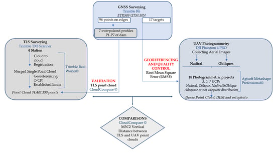
2. Materials and Methods
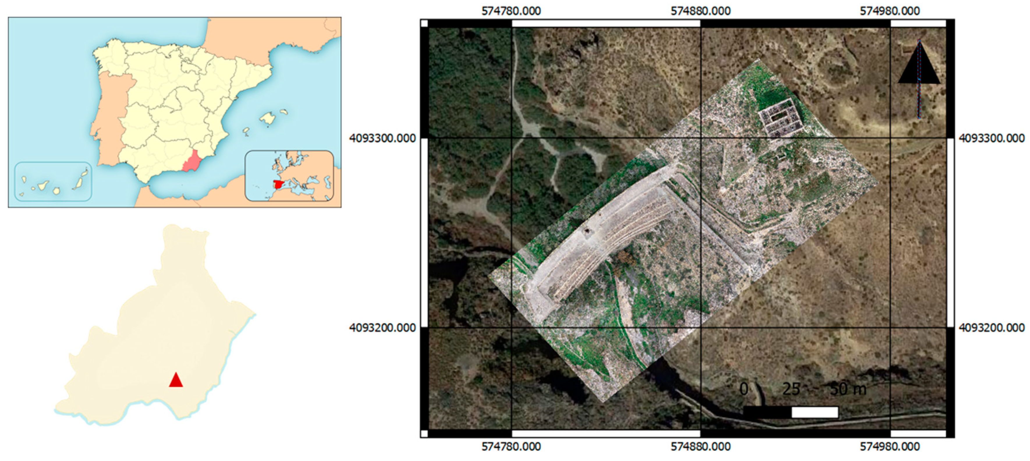
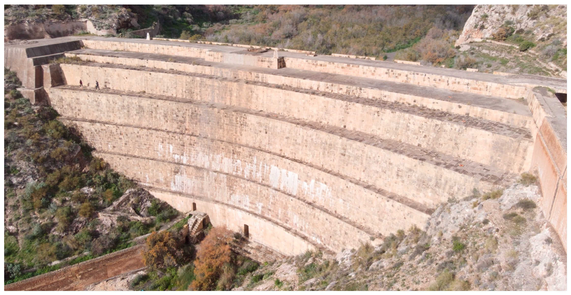
The flow followed in this work is shown in Figure 1. In summary, work begins with a global navigation satellite system (GNSS) survey of the dam edges and georeferencing targets. The points obtained on the dam edges are then used to interpolate seven profiles along the dam cross section that are then used to validate the point cloud obtained by the TLS. The targets are used indistinctly for the georeferencing of the 18 UAV photogrammetry projects and for quality control. Once the point clouds are obtained by UAV photogrammetry, they are compared with that obtained by TLS.

2.1. Study Site

The study area was centered on the Isabel II Dam (1841–1857), located in the province of Almería (Spain) about 7 km from the village of Níjar (Figure 2). Construction on the dam began with the foundation works in 1841, although it was not inaugurated until 8 May 1850 without the completion of the canals or offices, which would last until 1857. The reservoir was never completely filled, and the project failed due to several faults in the calculations made in the hydrological and pluviometric studies of the area.
However, this dam is one of the most spectacular, and simultaneously least known, elements of Spain’s hydraulic heritage. It is one of the few examples of the great hydraulic work undertaken in the 19th century, as well a key world reference for stone arch-gravity dams [43].
It was selected because of its downstream profile with walls that are very close to the vertical; its total height at its central point 31 m above the riverbed, as is shown in Figure 3.

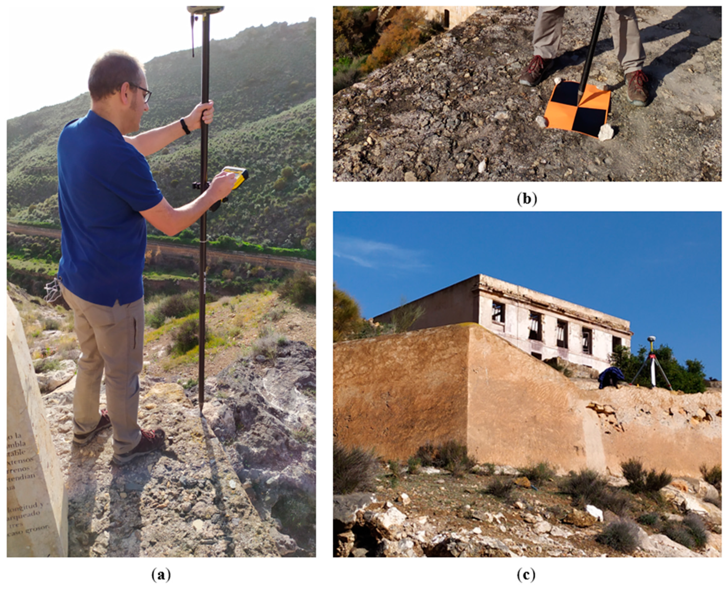
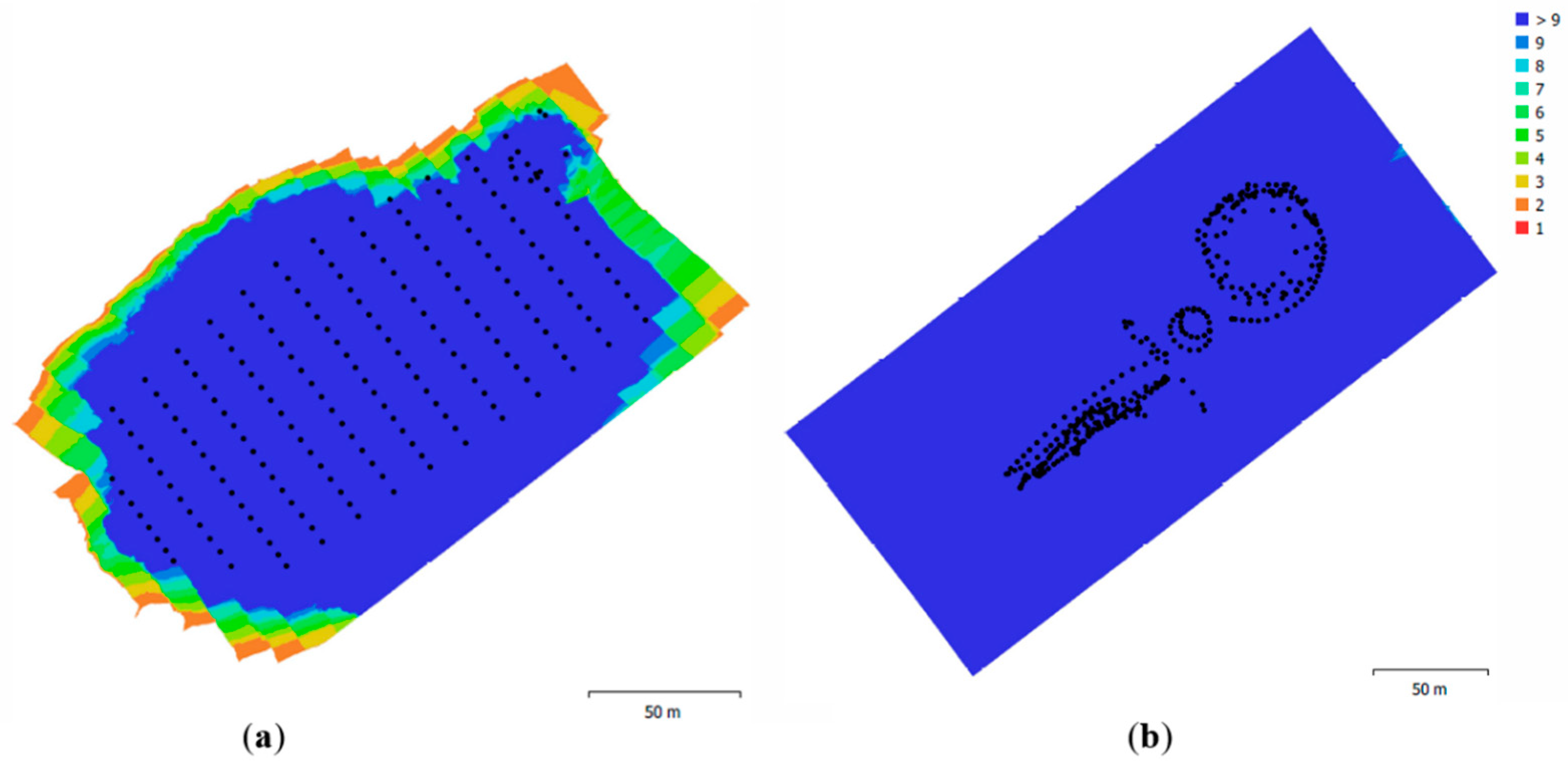
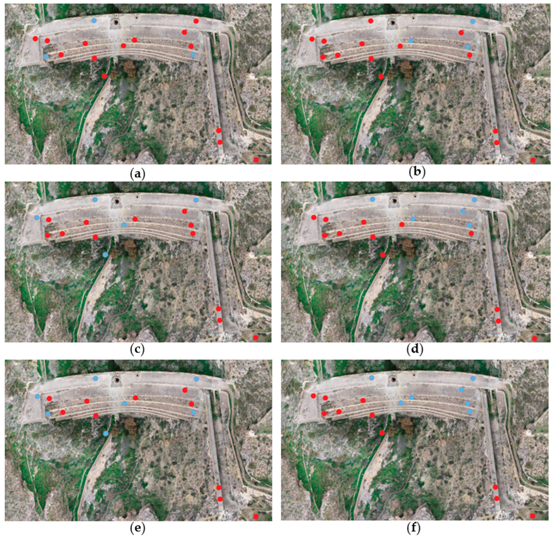
2.2. GNSS Surveying of Dam Edges and Ground Control Points

Before performing the photogrammetric flights and TLS scanning, a traditional GNSS survey was carried out, materializing a total of 113 points distributed along the dam’s downstream face, mostly on the edges of the steps, which allowed for their subsequent complete interpolation by means of cabinet work, as shown in Figure 4a. Of all these points, 17 were materialized by means of targets that allowed for their later viewing in photographs taken by the UAV. The targets used consisted of a red paper of size A3 (420 × 297 mm) with four quadrants, two of them black. Figure 4b shows an example of one of these targets. The three-dimensional (3D) coordinates of these targets were measured with a GNSS receiver operating in post-processing kinematic mode (PPK), with the base emitting corrections at a point near the dam, as shown in Figure 4c. Both rover and base GNSS receivers were Trimble R6 systems. The 3D coordinates of the base, corrected via the Trimble Centerpoint RTX Post-Processing Service, were 574909.418, 4093250.721, and 372.012 m (European Terrestrial Reference System 1989, ETRS89 and EGM08 geoid model).
From the data obtained by GNSS, seven theoretical profiles were made along the entire downstream face of the dam, numbered P1 to P7. These theoretical profiles obtained by GNSS are shown in Figure 5.

2.3. Topographic Surveying Using TLS

In order to meet the objective of this research, it was necessary to obtain a complete point cloud of the study area that would allow its later comparison with the products obtained by UAV photogrammetry. To this end, a complete scan of the dam’s downstream face was carried out using TLS.
The TLS provides a three-dimensional quasi-constant point cloud of the observed objects. The accuracy of this point cloud depends mainly on the distance between the scanner and the observed object. In recent years, the application of this equipment is increasing exponentially [44,45,46,47]. TLS measurements are based on the time elapsed by a laser ray emitted by the scanner and reflected by the object. From the time measurement, the distance is obtained and transformed into real-time coordinates. The working guidelines are described in depth in [48].

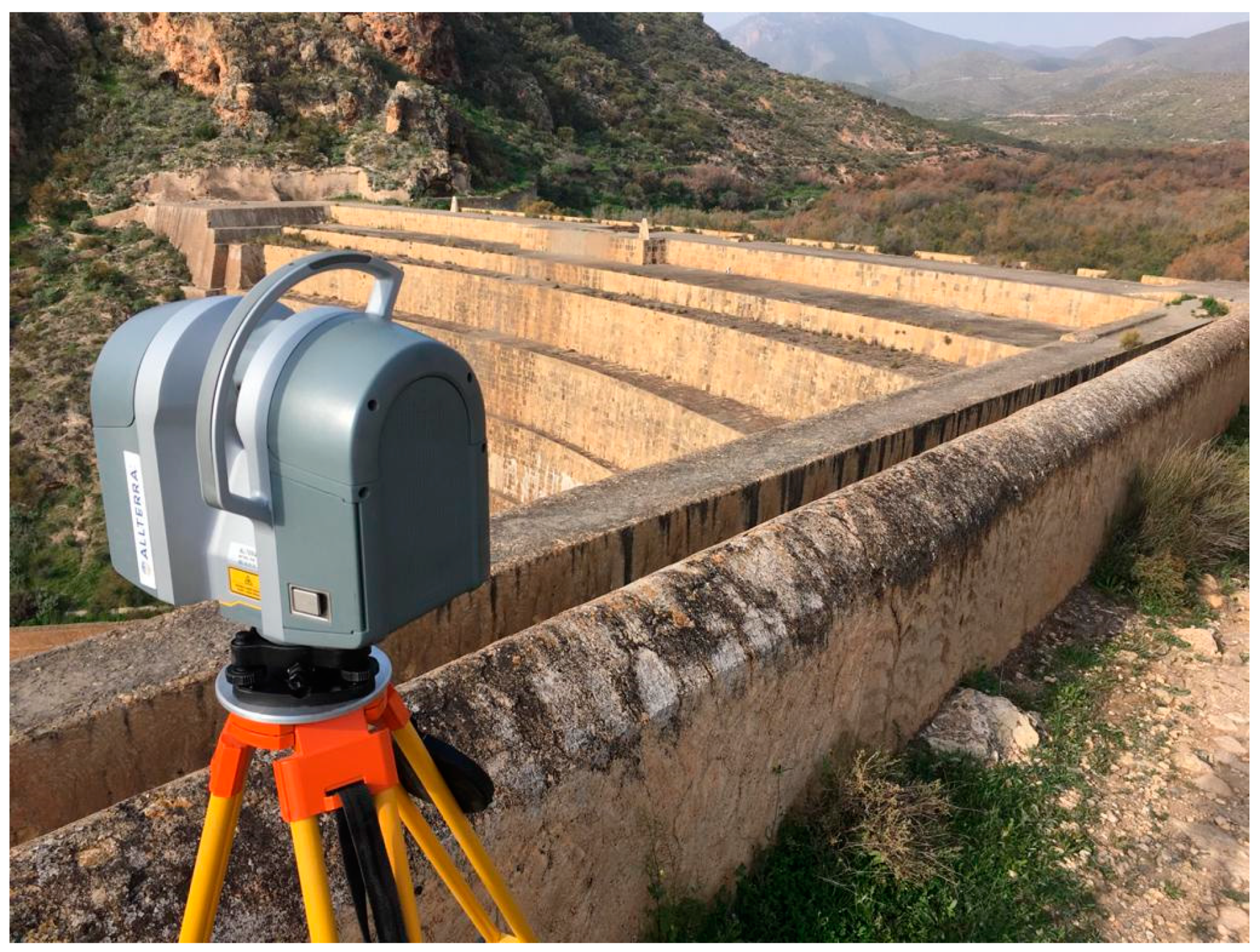
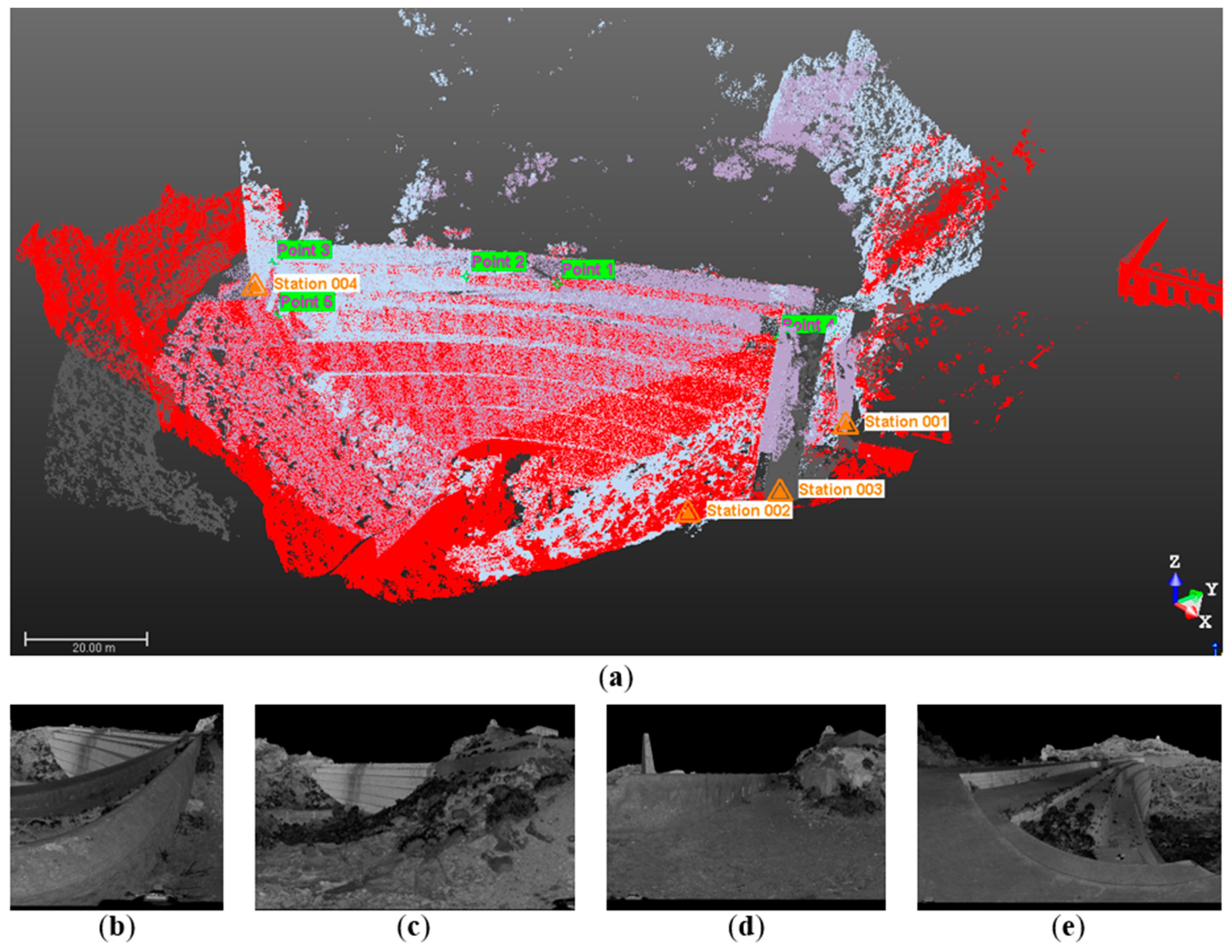
2.3.1. Data Acquisition

In this paper, a Trimble TX8 Scanner (Figure 6) was utilized for the topographical survey of the dam. This scanner measures almost 1 million points per second and its maximum scanning range is 120 m, but can extend up to 340 m under favorable conditions. The wavelength of the laser is 1.5 μm, and the scanning frequency is 1 MHz. Advertised measurement accuracy is ±2 mm, and the angular resolution is 0.07 mrad. It also includes an integrated HDR camera with 10 MP resolution. This scanner was used by [49] to measure the deflections of a technological suspension bridge above the Odra River (Southern Poland).
Due to the geometry of the study area, it was not possible to capture the entire wall from a single location. Therefore, the measurements for the TLS point cloud acquisition were taken from four different station points, as shown in Figure 7.
The point cloud for Station 1 had a total of 57,348,448 points. Station 2 had 119,268,180 points, Station 3 had 96,323,508 points, and Station 4 had 274,417,074 points.

2.3.2. Data Processing

Processing of the point clouds obtained by TLS was carried out using Trimble RealWorks software. The first step carried out once the clouds were loaded was the relative registration between them. To obtain a fine registration of all TLS datasets, cloud-to-cloud registration was used. This required searching for common tie points between each pair of clouds. Then, the four point clouds were merged into a single point cloud. This processing methodology was used by [50] who reported errors between 11–19 mm, [51] with an error of 13 mm, or [52] where a maximum error of 42 mm was found between scans from two different stations. The results of the registration of this work are shown in Table 1.
Once registration of the four scanning stations was complete, the indirect georeferencing of the merged point cloud was carried out in absolute coordinates using the ETRS89 UTM zone 30 N reference system. For this purpose, five control points were used, measured by GNSS, the position of which is shown in Figure 7a. The results of the indirect georeferencing adjustment are shown in Table 2.
The final TLS point cloud resulting from combining the four individual point clouds can also be seen in Figure 7a. To reduce the size of the resulting point cloud, limits were established according to the area of interest, resulting in a point cloud of 74,447,399 points.

2.4. Topographic Surveying Using UAV Photogrammetry

2.4.1. Image Capture

The images used in this study were captured by a rotary wing with four rotors, DJI Phantom 4 Pro UAV. This equipment has a navigation system that uses GPS and GLONASS. In addition, it is equipped with front, rear, and lower vision systems that allow it to detect surfaces with defined patterns and adequate lighting and avoid obstacles with a range between 0.2 and 7 m. The Phantom 4 RGB camera is equipped with a one-inch, 20-megapixel (5472 × 3648) sensor and has a manually adjustable aperture (from F2.8 to F11). The lens has a fixed focal length of 8.8 mm and a horizontal field of view (FOV) of 84°. The acquisition of photographs from a UAV takes place via airborne photogrammetry from the aircraft, whereby a block of photographs is taken from parallel flight lines that are flown in a snake pattern at a stable altitude with constant overlap and a vertical camera angle (90°) [53]. However, the integration of oblique photographs can reduce the systematic deformation resulting from inaccurate calculations to determine the internal geometry of the camera in modern SfM–MVS photogrammetry [54,55]. There is evidence that oblique photographs contribute to the integrity of the point cloud reconstruction [51,56]. For example, [51] studied the influence of the angle of the oblique images, ranging from 0–35°, and compared it with the TLS. They concluded that oblique images are indispensable to the improvement of accuracy and the decreasing of systematic errors in the endpoint cloud. The results also suggested that oblique camera angles of between 20 and 35° increased accuracy by almost 50%, in relation to blocks with only nadir images.
The images were obtained from two independent flights. The first was carried out in automatic pilot mode through the DJI GS Pro application, and a total of 207 nadir photographs were obtained in 13 passes. The flight height was set at 36 m above the dam crest, which is equivalent to a ground sample distance (GSD) of 1.3 cm. To obtain side and forward overlaps of 65% and 80%, respectively, the camera took a shot every two seconds. The second flight was made in manual mode to obtain oblique photographs, in order to provide photographic capture of all the details of the dam´s geometry. This flight was carried out at an approximate distance of 30 m from the downstream face of the dam and was executed in seven different passes, parallel to the dam and at varying altitudes. A total of 372 photographs (including those of the control building and the guard, which are not relevant to this study) were taken. In addition, due to the camera’s wide FOV, it was possible to cover the entire dam without going too far away from it. To avoid the appearance of the horizon in the photographs, an inclination angle of about 45° was adopted. No frontal photographs were taken, as much of the study area had horizontal surfaces. A total of 579 photographs with different points of view and scales were used to process the photogrammetric projects. Figure 8 shows the image overlap and camera locations for both flights.

2.4.2. Image Processing

The photogrammetric projects were executed using Agisoft Metashape Professional software, version 1.6.1.10009. This software is based on the SfM algorithm and runs in three independent steps. In the first step, all images are aligned by identifying and tying common points. During this process, the software estimates the camera’s internal and external orientation parameters, including non-linear radial distortion. The software only needs the focal length value, which it obtains directly from the EXIF data of the photographs. This was carried out with the PhotoScan accuracy set to “medium” in order to reduce the processing time. The result of this step is the camera position and orientation, as well as the internal calibration parameters and the 3D relative coordinates of a sparse point cloud in the area of interest. In the second step, the sparse point cloud is referred to an absolute coordinate system, in our case ETRS89 UTM 30N, and the point cloud is densified, once the optimization and adjustment of the camera model have been completed. This was also carried out with the PhotoScan accuracy set to “medium”. This point cloud needs to be cleaned up to eliminate all of the wild points not belonging in the model, which is done manually. The result is a highly detailed point cloud. From this point cloud, a mesh can be obtained; in this study, this was done using the height field method. In the third step, texture is applied to the mesh, and finally the orthophoto, digital surface model (DSM) and point cloud can be exported, in *.las formats. The bundle adjustment can be carried out using at least three ground control points (GCPs), but more accurate results can be obtained if more GCPs are used; thus, it is recommended that more GCPs be used to obtain optimal accuracy [57,58]. In this study, 17 targets placed on the dam were used as GCPs to georeference the project. The remaining targets not used in the bundle adjustment were used as control points (CPs) to evaluate the photogrammetric project accuracy, according to the root mean square error (RMSE) formula, described in [35]. There are numerous studies in which it has been corroborated that increasing the number of GCPs improves the accuracy of results of UAV photogrammetric projects. For example, [59] needed approximately six to seven GCPs to obtain accuracy of about 15.6 cm, and specified that it was necessary to increase the number of GCPs to reduce error. In [60], a study was conducted to analyze the optimal number of GCPs for volumetric measurements in open pit mines; for accuracies of about 5.0 cm, they concluded that about 15 GCP/km2 were needed. In [61], an extensive study was carried out with over 3000 combinations, concluding that an increase in GCPs improves accuracy, with a limited project ground sample distance (GSD). In addition, [62] studied the influence of GCP distribution on the accuracy obtained in photogrammetric projects and concluded that the vertical error is proportional to distance, to the nearest GCP. In their case, they obtained vertical RMSEs that ranged from 15.6 cm for three GCPs to 5.9 cm for 101 GCPs.
In total, 18 photogrammetric projects were carried out, differentiating the types of orientation used in the photographs (nadiral, oblique, or both), the number of GCPs used for georeferencing (3, 5, and 7), and an adequate or inadequate distribution of GCPs, according to [41], who established that an adequate distribution of GCPs is one in which GCPs are arranged at the edge of the study area, while the interior area is covered homogeneously with GCPs; distributions of GCPs that do not meet these criteria are considered inadequate. Table 3 shows a summary of the executed photogrammetric projects, and Figure 9 shows the different combinations of numbers of GCPs and type of distribution of the GCPs.

2.4.3. Accuracy Assessment

The evaluation of the accuracy was carried out by measuring the values of RMSEX, RMSEY, and RMSEZ, as well as RMSET (total error) measured on each CP.

2.5. Point Cloud Management

Prior to the above, and in order to compare the profiles obtained from GNSS with the point cloud obtained from TLS, the cloud-to-mesh (C2M) tool, offered by CloudCompare v2.8 [63], was used. The mesh was first obtained from the point cloud of the TLS, using the Dalaunay 2.5 tool, and once obtained, the C2M algorithm was applied to corroborate the adequate georeferencing of the TLS cloud and its validity for use as a reference for comparison against photogrammetric projects.
A multiscale model-to-model cloud comparison (M3C2) tool was used to compare the point clouds generated by the photogrammetric projects with the point cloud generated by the TLS. This tool calculates in a robust way, the distance, positive or negative, between two point clouds [64]. The principles of operation of this tool are described in [41]. M3C2 output consists of, amongst other data, a text file with the x-, y-, and z-coordinates for each point of the reference cloud and the 3D distance associated with the comparison. All data can be displayed using a color scale to highlight the resulting scalar field.

3. Results

3.1. Validation of Data Derived From TLS in Comparison With Theoretical Profiles Obtained by GNSS

Table 4 shows a summary of the comparison between the profiles obtained by GNSS and the model derived from the point cloud obtained by TLS. For the seven profiles studied, the average of the mean differences is below 0.03 cm with a standard deviation of less than 3 cm, which ensures the correct georeferencing of the TLS point cloud.
Figure 10a graphically represents the differences across the seven profiles obtained by GNSS with respect to the model derived from the point cloud obtained by TLS. Figure 10b shows an example of the error distribution for Profile 2, in which it can be seen that most of the differences are close to 0 and that, in some cases, larger errors appeared in most cases due to the presence of shrubs growing on the dam face, as shown in Figure 10c.

3.2. RMSE UAV-PhotogrAmmetric Projects

Figure 11 shows the precision results obtained in the 18 photogrammetric projects through the evaluation of the RMSE.
From the analysis of the data obtained, it is clear that an adequate distribution of GCPs is important for the minimization of errors. The results obtained were in line with those obtained by [41]. Therefore, the average error in the projects with inadequate distribution was around 8.5 cm, while in the projects with adequate distribution, it was in an average of 4.0 cm, which represents an improvement of more than 50%. As indicated in [57], increasing the number of GCPs improves the accuracy of photogrammetric projects, regardless of whether the distribution of GCPs is adequate or not. In this study, a slight worsening was found for 7 GCPs against 5 GCPs. Thus, for 3 GCPs the average error was 7.1, for 5 GCPs it was 5.5, and for 7 GCPs it was 6.2 cm. This alteration was only found for the projects with inadequate distribution, while for the projects with adequate distribution, the error decreased as the number of GCPs increased. Thus, for 3 GCPs the average error was 4.8, for 5 GCPs it was 4.0, and for 7 GCPs it was 3.3 cm. Regarding the orientation of the photographs, an average error of 7.9 was obtained for projects with nadiral photographs, 5.0 for projects with oblique photographs, and 6.0 cm for projects that combined both orientations of photographs. For the projects with inadequate distribution, the best results were obtained for oblique photographs with an average of 6.2 cm. However, for an adequate distribution, the best results were obtained for nadiral photographs with an average of 3.7 as opposed to 3.8 obtained for oblique photographs, or 4.6 cm for projects that combined both orientations.

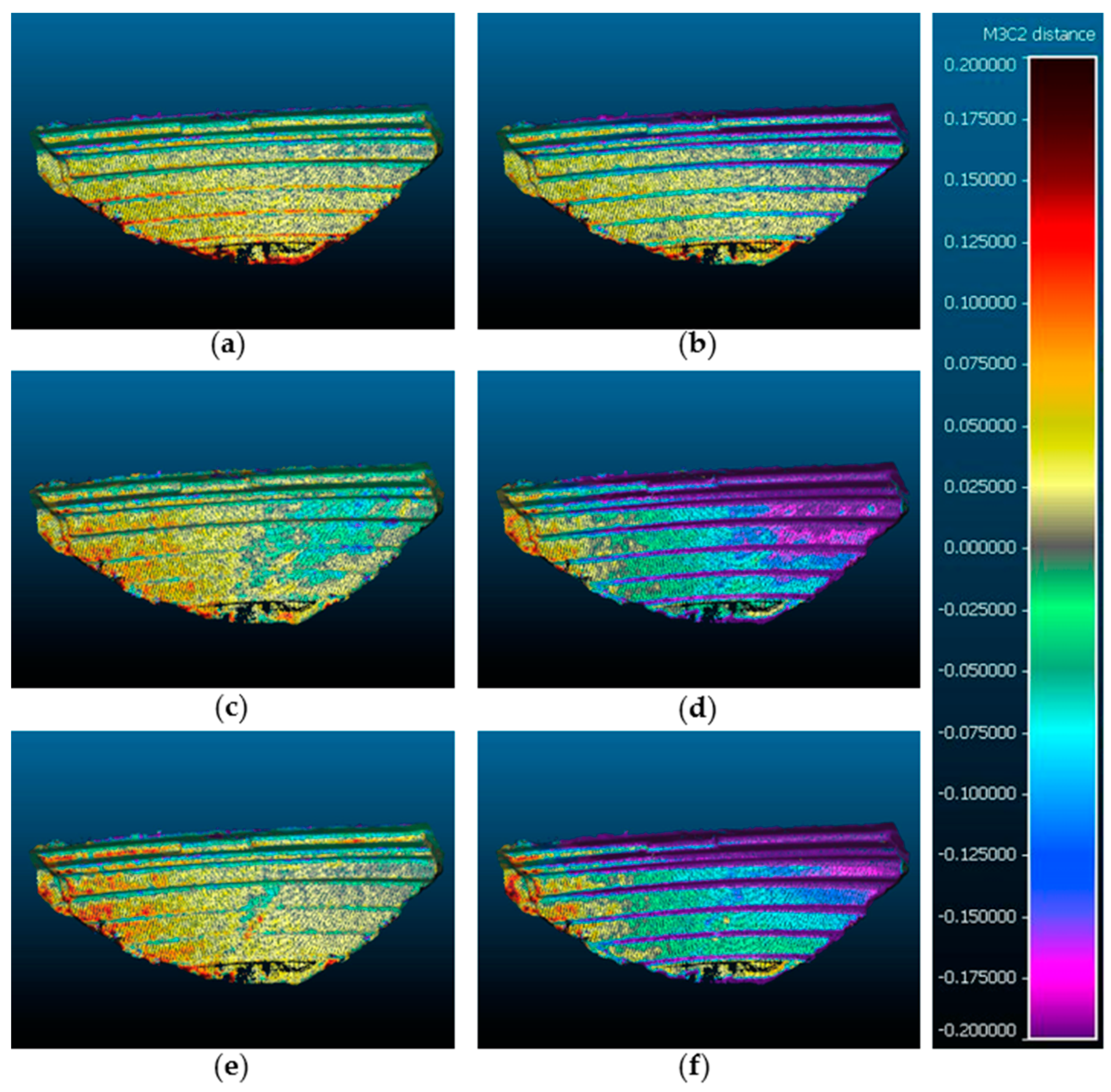
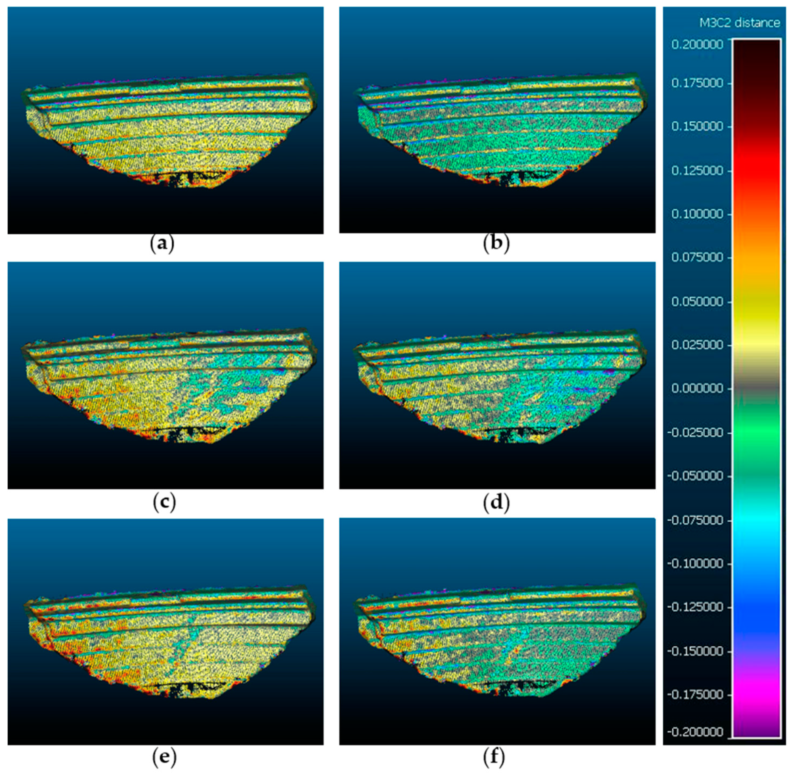
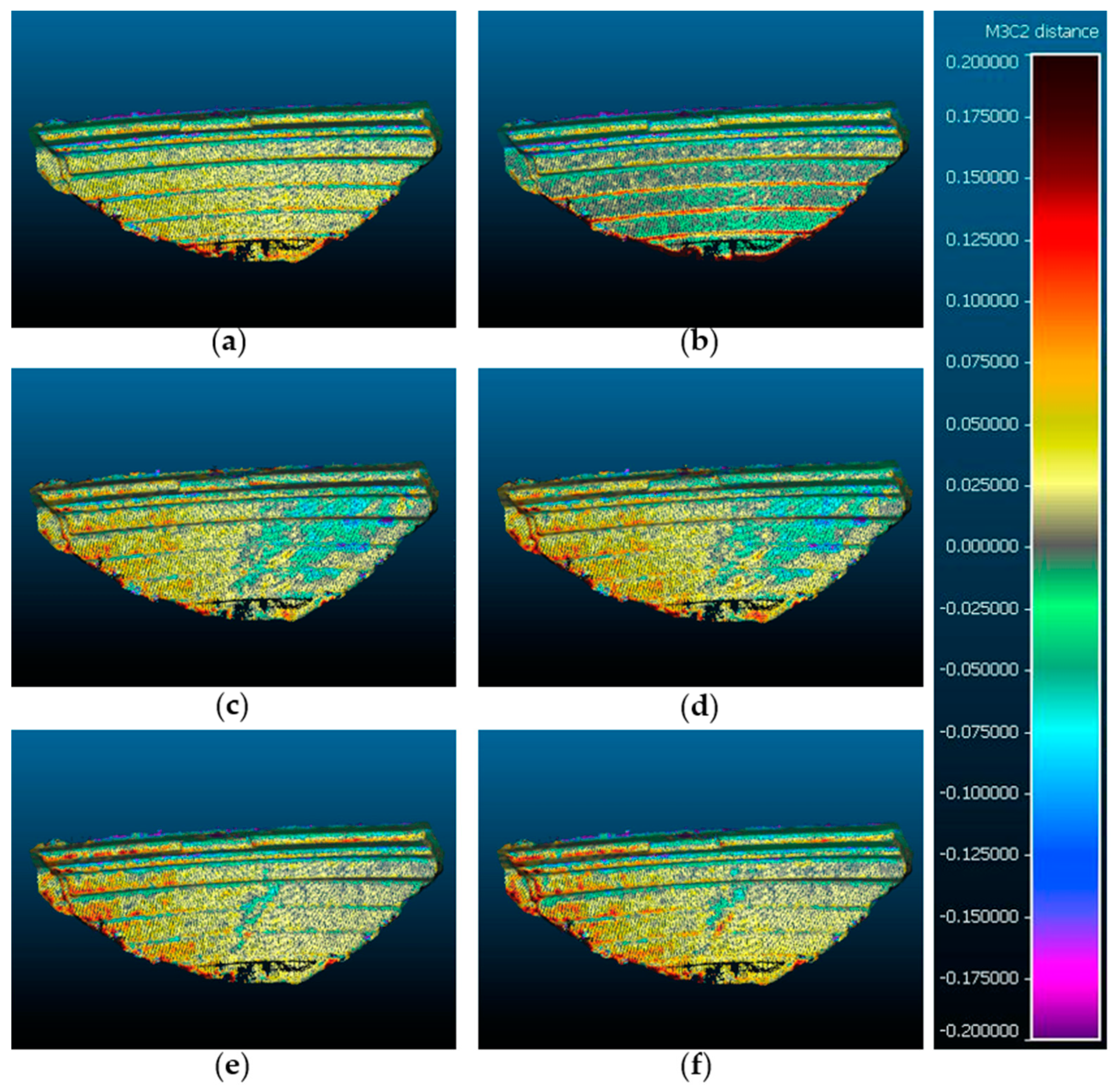
3.3. Vertical Distances between the Point Clouds Obtained by TLS and UAV Photogrammetry

For all studied scenarios, the point clouds were evaluated based on reference data acquired by the TLS. There are several studies in scientific literature concerning the evaluation of vertical distances between clouds obtained by UAV photogrammetry and reference clouds. For example, [65] evaluated the capacity of UAV photogrammetry to obtain point clouds in quarries where there were walls with near-vertical inclination. In this study, they corroborated the improvement in the description of the break lines and in the accuracy of cross profiles with vertical walls, using oblique photographs and comparing the UAV photogrammetry clouds with the profiles obtained by a total station. One of their main conclusions was that the scenario with nadir photographs resulted in smoother geometry and a more gradual transition between vertical and horizontal surfaces than the scenario involving nadir and oblique photographs.
Figure 12 shows the vertical distances between the cloud obtained by TLS and the six UAV photogrammetry projects executed with 3 GCPs. For the projects with nadiral photographs and adequate distribution of GCPs, the M3C2-calculated vertical distances resulted in absolute values distributed as a Gaussian function with mean = −0.075 and standard deviation (SD) = 8.335 cm. For the project with nadiral photographs and inadequate distribution of GCPs, a mean distance of −7.806 and an SD of 13.586 cm were obtained. For the project with oblique photographs and adequate distribution of GCPs, an average distance of 0.068 and an SD of 6.406 cm were obtained. For the project with oblique photographs and inadequate distribution of GCPs, an average distance of −21.597 and an SD of 22.466 cm were obtained. For the project with nadiral and oblique photographs and adequate distribution of GCPs, a mean distance of 0.195 and an SD of 7.066 cm were obtained. For the project with nadiral and oblique photographs and inadequate distribution of GCPs, an average distance of −24.692 and an SD of 26.988 cm were obtained. For this scenario, with inadequate distribution, the use of oblique photographs increased the average absolute distance between the clouds by 47%. However, for an adequate distribution, there was a reduction of the average cloud distance by 30%.
Figure 13 shows the vertical distances between the cloud obtained by TLS and the six UAV photogrammetry projects executed with 5 GCPs. For the project with nadiral photographs and adequate distribution of GCPs, an average distance of 0.492 and an SD of 7.236 cm were obtained. For the project with nadir photographs and inadequate distribution of GCPs, a mean distance of −3.015 and an SD of 7.501 cm were obtained. For the project with oblique photographs and inadequate distribution of GCPs, a mean distance of 1.109 and an SD of 6.092 cm were obtained. For the project with oblique photographs and inadequate distribution of GCPs, a mean distance of −1.418 and an SD of 6.303 cm were obtained. For the project with nadiral and oblique photographs and adequate distribution of GCPs, a mean distance of 1.361 and SD of 6.593 m were obtained. For the project with nadiral and oblique photographs and inadequate distribution of GCPs, a mean distance of −1.666 and SD of 6.661 cm were obtained. For this scenario, with inadequate distribution, the use of oblique photographs reduced the absolute average distance between the clouds by 25%, and by 9% for adequate distribution.
Figure 14 shows the vertical distances between the cloud obtained by TLS and the six UAV photogrammetry projects executed with 7 GCPs. For the project with nadiral photographs and adequate distribution of GCPs, an average distance of 0.325 and SD of 7.226 cm were obtained. For the project with nadiral photographs and inadequate distribution of GCPs, a mean distance of −0.637 and SD of 8.689 cm were obtained. For the project with oblique photographs and adequate distribution of GCPs, a mean distance of 0.704 and SD of 6.187 cm were obtained. For the project with oblique photographs and inadequate distribution of GCPs, a mean distance of 1.134 and SD of 6.616 cm were obtained. For the project with nadiral and oblique photographs and adequate distribution of GCPs, a mean distance of 1.130 and a SD of 6.579 cm were obtained. For the project with nadiral and oblique photographs and inadequate distribution of GCPs, a mean distance of 1.314 and SD of 7.143 cm were obtained. For this scenario, with inadequate distribution, the use of oblique photographs reduced the absolute average distance between the clouds by 18%, and by 11% for adequate distribution.

4. Discussion

Considering that the accuracy error of measurements made with GNSS was about 8 for the horizontal plane and 15 mm vertically, the adjustment obtained for the TLS point cloud is considered adequate, since the average adjustment error obtained at the control points was 25 mm. In turn, the maximum cloud-to-cloud error found in the four-station registry was below 5 mm, similar to that obtained by [50,51], and much less than that reported by [52]. Analyzing the differences with respect to the seven theoretical profiles obtained by GNSS, a mean error of −0.030 and a standard deviation (SD) of 2.965 cm were found. Similar errors were obtained by [66], who reported three different experiments to obtain indirect georeferencing of TLS point clouds by using control lines. The results they found ranged from a mean error of 0.002–0.064 and a SD between 0.928 cm and 1.729 cm. Therefore, in view of the results obtained for the adjustment and georeferencing of the point cloud by TLS, it can be adopted as a reference cloud for subsequent comparison with projects obtained by UAV photogrammetry.
Regarding the number of GCPs used for the georeferencing of photogrammetric projects, in this study, a clear trend of improved results was obtained by increasing the number of GCPs, with the only noteworthy change being for an inadequate distribution of the seven GCPs. This is approximately 50% less obvious with oblique photographs than with nadiral photographs, which demonstrates the need to incorporate oblique photographs when it is not possible to have an adequate distribution of GCPs.
According to [62], the results of our study show similar values, where, for three GCPs and an inadequate distribution, an RMSE of 9.49 cm was obtained, while with an increase of GCPs and improved distribution the RMSE decreased to 3.32 cm. This same trend is observed regardless of the orientation of the photographs.
In recent years, studies on the benefit of introducing oblique images or an adequate distribution of GCPs in UAV photogrammetry projects are common. However, there have been only few such studies applied to quasi-vertical or vertical walls. In [55], it is noted that for the network of self-calibrated images to be accurate, the spatial distribution of GCPs needs to cover the whole area of interest. In turn, the density of GCPs depends on the accuracy needed in the project, the geometry of the network, and the quality of the photographs. For example, to obtain accuracies of 5.0 cm, at a height of 100 m (GSD 23 mm), about 15 GCPs were needed, with an average minimum spacing of 50 m. They pointed out that improving the network geometry with oblique images or with a precisely pre-calibrated camera could reduce the number of GCPs. These results coincide with those obtained in this study, especially when the distribution of GCPs was inadequate. However, when the number of GCPs was increased to five or seven, and the distribution was adequate, no improvement was found with the use of oblique photographs. For projects with inadequate distribution, the use of nadir photographs dramatically worsens the results. In this case, nadir photographs do not have such a strong effect when combined with oblique photographs. In the case of adequate distribution, the opposite happens; the best results are obtained with nadir photographs, while in this case, oblique photographs slightly worsen the results.
As noted in [67], the accuracy does not only depend upon the number of GCPs, but also on their distribution pattern. Therefore, the choice of a suitable pattern and the number of GCPs for a particular mission can help obtain sufficiently accurate results with economic feasibility. In their study, the accuracy ranged from 18.2 with three GCPs to 11.3 cm with nine GCPs. They also highlighted the importance of positioning a GCP in the central region of the area. There was a substantial improvement in accuracy due to the addition of another GCP in the central area. Our study has improved those results, where, for three GCPs and an adequate distribution, the average error was 4.8 cm. In [42], the authors studied the acquisition and use of oblique images for the 3D reconstruction of a historical building, obtained by UAV for the realization of a high-level-of-detail architectural survey. For this purpose, they used several software applications, obtaining similar results, in which the differences with respect to a reference cloud ranged from 0.3–2.5 to 1.6–3.9 cm. As demonstrated in [68], the use of oblique images obtained from a low-cost UAV system and processed by SfM software was an effective method for surveying cultural heritage sites. In particular, they studied a facade, in which they obtained an average distance between the clouds (UAV vs TLS) of 4.0 cm, with an SD of 9.0 cm. Similar results were found in our study, where, for an adequate distribution of GCPs, the mean value ranged from −0.1 to 1.4 cm with an SD ranging from 6.1 to 8.3 cm.
With respect to the break lines referred to by [65], this fact can be visually corroborated with reference to Figure 11, Figure 12 and Figure 13, wherein the major differences can be seen in the edges, at which abrupt changes of slope occur. According to [51], in our study, evaluating the vertical distances between the UAV photogrammetry cloud and the TLS cloud, the use of oblique photographs improved results by between 9% and 30% for all scenarios except three GCPs and inadequate distribution.

5. Conclusions

The SfM analysis of the UAV images is a valuable and verified tool for surveyors interested in the high-resolution reconstruction of nearly vertical walls. UAV studies are also a useful tool for risk management in accessing hazardous and inaccessible areas, such as in cases of slope cuttings on highways or roads with near vertical inclination or the analysis of architectural facades in cities. This study has addressed the influence of three factors: The number of GCPs, the distribution of GCPs, and the orientation of photographs obtained by the UAV. From the results obtained, a series of guidelines can be established to simplify the process of capturing data in the field and to improve the accuracy of photogrammetric products. In order to obtain optimal results with respect to accuracy, it is important to distribute of as many GCPs as possible throughout the study area and to make use of an adequate distribution GCPs coverage, as far as possible, over the entire area of interest. In case these two conditions are difficult to meet, the inclusion of oblique photographs in the photogrammetric project results in a substantial improvement in the results obtained. In this way, it is possible to achieve an RMSE of around 3.0 cm, which is a sufficient scale for most engineering or architectural projects. In addition, oblique photographs ostensibly improve the geometric description of break lines or sudden changes in slope. Therefore, it is always advisable to use them for projects with vertical topography. Under these circumstances, UAV photogrammetry constitutes a technique whose results are equivalent to those obtained by a TLS, but with the incentive of lower cost and greater facility for the treatment of the point cloud.

Author Contributions

The contributions of the authors were: Conceptualization, P.M.-C., F.C.-R. and F.A.-V.; methodology, P.M.-C., F.C.-R. and F.A.-V.; software P.M.-C.; validation, P.M.-C.; formal analysis, P.M.-C., F.C.-R. and F.A.-V.; investigation, P.M.-C., F.C.-R. and F.A.-V.; resources, F.C.-R. and F.A.-V.; writing—original draft preparation, P.M.-C.; writing—review and editing, P.M.-C., F.C.-R. and F.A.-V.; visualization, P.M.-C.; project administration, F.C.-R. and F.A.-V. All authors have read and agreed to the published version of the manuscript.

Funding

This research received no external funding.

Conflicts of Interest

The authors declare no conflict of interest.

References

  1. Wallace, L.O.; Lucieer, A.; Malenovsky, Z.; Turner, D.; Vopěnka, P. Assessment of Forest Structure Using Two UAV Techniques: A Comparison of Airborne Laser Scanning and Structure from Motion (SfM) Point Clouds. Forests 2016, 7, 62. [Google Scholar] [CrossRef] [Green Version]
  2. Koo, J.-B. The Study on Recording Method for Buried Cultural Property Using Photo Scanning Technique. J. Digit. Contents Soc. 2015, 16, 835–847. [Google Scholar] [CrossRef] [Green Version]
  3. Yao, H.; Qin, R.; Chen, X. Unmanned Aerial Vehicle for Remote Sensing Applications—A Review. Remote Sens. 2019, 11, 1443. [Google Scholar] [CrossRef] [Green Version]
  4. Liu, P.; Chen, A.Y.; Huang, Y.-N.; Han, J.-Y.; Lai, J.-S.; Kang, S.-C.; Wu, T.-H.; Wen, M.-C.; Tsai, M.-H. A review of rotorcraft Unmanned Aerial Vehicle (UAV) developments and applications in civil engineering. Smart Struct. Syst. 2014, 13, 1065–1094. [Google Scholar] [CrossRef]
  5. Bento, M.D.F. Unmanned Aerial Vehicles: An Overview. InsideGNSS 2008, 3, 54–61. [Google Scholar]
  6. Samad, A.M.; Kamarulzaman, N.; Hamdani, M.A.; Mastor, T.A.; Hashim, K.A. The potential of Unmanned Aerial Vehicle (UAV) for civilian and mapping application. In Proceedings of the 2013 IEEE 3rd International Conference on System Engineering and Technology, Shah Alam, Malaysia, 19–20 August 2013; Institute of Electrical and Electronics Engineers (IEEE): Piscataway, NJ, USA, 2013; pp. 313–318. [Google Scholar]
  7. Mesas-Carrascosa, F.-J.; Pérez-Porras, F.; De Larriva, J.E.M.; Frau, C.M.; Agüera-Vega, F.; Carvajal-Ramirez, F.; Carricondo, P.J.M.; García-Ferrer, A. Drift Correction of Lightweight Microbolometer Thermal Sensors On-Board Unmanned Aerial Vehicles. Remote Sens. 2018, 10, 615. [Google Scholar] [CrossRef] [Green Version]
  8. Grenzdörffer, G.; Engel, A.; Teichert, B. The photogrammetric potential of low-cost UAVs in forestry and agriculture. Int. Arch. Photogramm. Remote Sens. Spat. Inf. Sci. 2008, XXXVII(Part B1), 1207–1214. [Google Scholar]
  9. Tian, J.; Wang, L.; Li, X.; Gong, H.; Shi, C.; Zhong, R.; Liu, X. Comparison of UAV and WorldView-2 imagery for mapping leaf area index of mangrove forest. Int. J. Appl. Earth Obs. Geoinf. 2017, 61, 22–31. [Google Scholar] [CrossRef]
  10. Kachamba, D.; Ørka, H.O.; Gobakken, T.; Eid, T.; Mwase, W. Biomass Estimation Using 3D Data from Unmanned Aerial Vehicle Imagery in a Tropical Woodland. Remote Sens. 2016, 8, 968. [Google Scholar] [CrossRef] [Green Version]
  11. Carvajal-Ramirez, F.; Da Silva, J.M.; Agüera-Vega, F.; Carricondo, P.J.M.; Serrano, J.; Moral, F.J. Evaluation of Fire Severity Indices Based on Pre- and Post-Fire Multispectral Imagery Sensed from UAV. Remote Sens. 2019, 11, 993. [Google Scholar] [CrossRef] [Green Version]
  12. Yuan, C.; Zhang, Y.; Liu, Z. A survey on technologies for automatic forest fire monitoring, detection, and fighting using unmanned aerial vehicles and remote sensing techniques. Can. J. For. Res. 2015, 45, 783–792. [Google Scholar] [CrossRef]
  13. Carricondo, P.J.M.; Carvajal-Ramirez, F.; Yero-Paneque, L.; Vega, F.A. Combination of nadiral and oblique UAV photogrammetry and HBIM for the virtual reconstruction of cultural heritage. Case study of Cortijo del Fraile in Níjar, Almería (Spain). Build. Res. Inf. 2019, 48, 140–159. [Google Scholar] [CrossRef]
  14. Carvajal-Ramirez, F.; Navarro-Ortega, A.D.; Agüera-Vega, F.; Martínez-Carricondo, P.; Mancini, F. Virtual reconstruction of damaged archaeological sites based on Unmanned Aerial Vehicle Photogrammetry and 3D modelling. Study case of a southeastern Iberia production area in the Bronze Age. Measurement 2019, 136, 225–236. [Google Scholar] [CrossRef]
  15. Doumit, J. Structure from motion technology for historic building information modeling of Toron fortress (Lebanon). Proc. Int. Conf. InterCarto InterGIS 2019, 25. [Google Scholar] [CrossRef]
  16. Salvo, G.; Caruso, L.; Scordo, A. Urban Traffic Analysis through an UAV. Proc. Soc. Behav. Sci. 2014, 111, 1083–1091. [Google Scholar] [CrossRef] [Green Version]
  17. Kanistras, K.; Martins, G.; Rutherford, M.J.; Valavanis, K.P. Survey of unmanned aerial vehicles (uavs) for traffic monitoring. In Handbook of Unmanned Aerial Vehicles; Valavanis, K.P., Vachtsevanos, G.J., Eds.; Springer Reference: Dordrecht, The Netherlands, 2015; ISBN 9789048197071. [Google Scholar]
  18. Eltner, A.; Mulsow, C.; Maas, H.-G. Quantitative Measurement of Soil Erosion from Tls And Uav Data. Int. Arch. Photogramm. Remote Sens. Spat. Inf. Sci. 2013, 119–124. [Google Scholar] [CrossRef] [Green Version]
  19. Piras, M.; Taddia, G.; Forno, M.G.; Gattiglio, M.; Aicardi, I.; Dabove, P.; Russo, S.L.; Lingua, A. Detailed geological mapping in mountain areas using an unmanned aerial vehicle: Application to the Rodoretto Valley, NW Italian Alps. Geomat. Nat. Hazards Risk 2016, 8, 137–149. [Google Scholar] [CrossRef]
  20. Pavlidis, G.; Koutsoudis, A.; Arnaoutoglou, F.; Tsioukas, V.; Chamzas, C. Methods for 3D digitization of Cultural Heritage. J. Cult. Heritage 2007, 8, 93–98. [Google Scholar] [CrossRef] [Green Version]
  21. Püschel, H.; Sauerbier, M.; Eisenbeiss, H. A 3D Model of Castle Landenberg (CH) from Combined Photogrametric Processing of Terrestrial and UAV Based Images. Int. Arch. Photogramm. Remote Sens. Spat. Inf. Sci. 2008, 37, 93–98. [Google Scholar]
  22. Themistocleous, K.; Agapiou, A.; Hadjimitsis, D. 3D Documentation And Bim Modeling of Cultural Heritage Structures using Uavs: The Case of the Foinikaria Church. Int. Arch. Photogramm. Remote Sens. Spat. Inf. Sci. 2016, 42, 45–49. [Google Scholar] [CrossRef] [Green Version]
  23. Aber, J.S.; Marzolff, I.; Ries, J.B. Small-Format Aerial Photography; Elsevier Science: Amsterdam, The Netherlands, 2010; ISBN 9780444532602. [Google Scholar]
  24. Atkinson, K.B. Close Range Photogrammetry and Machine Vision; Whittles Publishing: Dunbeath, UK, 2001; ISBN 978-1870325738. [Google Scholar]
  25. Fernández-Hernandez, J.; González-Aguilera, D.; Rodríguez-Gonzálvez, P.; Mancera-Taboada, J. Image-Based Modelling from Unmanned Aerial Vehicle (UAV) Photogrammetry: An Effective, Low-Cost Tool for Archaeological Applications. Archaeometry 2014, 57, 128–145. [Google Scholar] [CrossRef]
  26. Fonstad, M.A.; Dietrich, J.T.; Courville, B.C.; Jensen, J.L.; Carbonneau, P.E. Topographic structure from motion: A new development in photogrammetric measurement. Earth Surf. Process. Landf. 2013, 38, 421–430. [Google Scholar] [CrossRef] [Green Version]
  27. Javernick, L.; Brasington, J.; Caruso, B. Modeling the topography of shallow braided rivers using Structure-from-Motion photogrammetry. Geomorphology 2014, 213, 166–182. [Google Scholar] [CrossRef]
  28. Westoby, M.J.; Brasington, J.; Glasser, N.; Hambrey, M.; Reynolds, J. ‘Structure-from-Motion’ photogrammetry: A low-cost, effective tool for geoscience applications. Geomorphology 2012, 179, 300–314. [Google Scholar] [CrossRef] [Green Version]
  29. Snavely, N.; Seitz, S.M.; Szeliski, R. Modeling the World from Internet Photo Collections. Int. J. Comput. Vis. 2007, 80, 189–210. [Google Scholar] [CrossRef] [Green Version]
  30. Vasuki, Y.; Holden, E.-J.; Kovesi, P.; Micklethwaite, S. Semi-automatic mapping of geological Structures using UAV-based photogrammetric data: An image analysis approach. Comput. Geosci. 2014, 69, 22–32. [Google Scholar] [CrossRef]
  31. Furukawa, Y.; Ponce, J. Accurate, Dense, and Robust Multiview Stereopsis. IEEE Trans. Pattern Anal. Mach. Intell. 2009, 32, 1362–1376. [Google Scholar] [CrossRef]
  32. Lowe, D.G. Distinctive Image Features from Scale-Invariant Keypoints. Int. J. Comput. Vis. 2004, 60, 91–110. [Google Scholar] [CrossRef]
  33. Kamal, W.A.; Samar, R. A mission planning approach for UAV applications. In Proceedings of the 2008 47th IEEE Conference on Decision and Control, Cancun, Mexico, 9–11 December 2008; Institute of Electrical and Electronics Engineers (IEEE): Piscataway, NJ, USA, 2008; pp. 3101–3106. [Google Scholar]
  34. Hugenholtz, C.; Brown, O.; Walker, J.; Barchyn, T.E.; Nesbit, P.; Kucharczyk, M.; Myshak, S. Spatial Accuracy of UAV-Derived Orthoimagery and Topography: Comparing Photogrammetric Models Processed with Direct Geo-Referencing and Ground Control Points. Geomatica 2016, 70, 21–30. [Google Scholar] [CrossRef]
  35. Vega, F.A.; Carvajal-Ramirez, F.; Martínez-Carricondo, P. Accuracy of Digital Surface Models and Orthophotos Derived from Unmanned Aerial Vehicle Photogrammetry. J. Surv. Eng. 2017, 143, 04016025. [Google Scholar] [CrossRef]
  36. Amrullah, C.; Suwardhi, D.; Meilano, I. Product Accuracy Effect of Oblique and Vertical Non-Metric Digital Camera Utilization in Uav-Photogrammetry to Determine Fault Plane. ISPRS Ann. Photogramm. Remote Sens. Spat. Inf. Sci. 2016, 41–48. [Google Scholar] [CrossRef]
  37. Dandois, J.P.; Olano, M.; Ellis, E. Optimal Altitude, Overlap, and Weather Conditions for Computer Vision UAV Estimates of Forest Structure. Remote Sens. 2015, 7, 13895–13920. [Google Scholar] [CrossRef] [Green Version]
  38. Mesas-Carrascosa, F.-J.; Rumbao, I.C.; Berrocal, J.A.B.; García-Ferrer, A. Positional Quality Assessment of Orthophotos Obtained from Sensors Onboard Multi-Rotor UAV Platforms. Sensors 2014, 14, 22394–22407. [Google Scholar] [CrossRef] [PubMed]
  39. Vautherin, J.; Rutishauser, S.; Schneider-Zapp, K.; Choi, H.F.; Chovancova, V.; Glass, A.; Strecha, C. Photogrammetric Accuracy and Modeling of Rolling Shutter Cameras. ISPRS Ann. Photogramm. Remote Sens. Spat. Inf. Sci. 2016, 139–146. [Google Scholar] [CrossRef]
  40. Murtiyoso, A.; Grussenmeyer, P. Documentation of heritage buildings using close-range UAV images: Dense matching issues, comparison and case studies. Photogramm. Rec. 2017, 32, 206–229. [Google Scholar] [CrossRef] [Green Version]
  41. Carricondo, P.J.M.; Vega, F.A.; Carvajal-Ramirez, F.; Mesas-Carrascosa, F.-J.; García-Ferrer, A.; Pérez-Porras, F.-J. Assessment of UAV-photogrammetric mapping accuracy based on variation of ground control points. Int. J. Appl. Earth Obs. Geoinf. 2018, 72, 1–10. [Google Scholar] [CrossRef]
  42. Aicardi, I.; Chiabrando, F.; Grasso, N.; Lingua, A.M.; Noardo, F.; Spanò, A. Uav Photogrammetry with Oblique Images: First Analysis on Data Acquisition and Processing. ISPRS Int. Arch. Photogramm. Remote Sens. Spat. Inf. Sci. 2016, 835–842. [Google Scholar] [CrossRef]
  43. García-Sánchez, J.F. El pantano de Isabel II de Níjar (Almería): Paisaje, fondo y figura. ph Investig. 2014, 3, 55–74. [Google Scholar]
  44. Lovas, T.; Barsi, A.; Polgar, A.; Kibedy, Z.; Berenyi, A.; Detrekoi, A.; Dunai, L. Potential of terrestrial laserscanning in deformation measurement of structures. Am. Soc. Photogramm. Remote Sens. ASPRS Annu. Conf. 2008 Bridg. Horiz. New Front. Geospat. Collab. 2008, 2, 454–463. [Google Scholar]
  45. Danson, F.M.; Hetherington, D.; Koetz, B.; Morsdorf, F.; Allgöwer, B. Forest Canopy Gap Fraction from Terrestrial Laser Scanning. IEEE Geosci. Remote Sens. Lett. 2007, 4, 157–160. [Google Scholar] [CrossRef] [Green Version]
  46. Lumme, J.; Karjalainen, M.; Kaartinen, H.; Kukko, A.; Hyyppä, J.; Hyyppä, H.; Jaakkola, A.; Kleemola, J. Terrestrial laser scanning of agricultural crops. Int. Arch. Photogramm. Remote Sens. Spat. Inf. Sci. 2008, 47, 563–566. [Google Scholar]
  47. Abellan, A.; Calvet, J.; Vilaplana, J.M.; Blanchard, J. Detection and spatial prediction of rockfalls by means of terrestrial laser scanner monitoring. Geomorphology 2010, 119, 162–171. [Google Scholar] [CrossRef]
  48. Schulz, T. Calibration of a Terrestrial Laser Scanner for Engineering Geodesy. Geod. Metrol. Eng. Geod. 2007. [Google Scholar] [CrossRef]
  49. Kwiatkowski, J.; Anigacz, W.; Beben, D. Comparison of Non-Destructive Techniques for Technological Bridge Deflection Testing. Materials 2020, 13, 1908. [Google Scholar] [CrossRef]
  50. Fryskowska, A. Accuracy Assessment of Point Clouds Geo-Referencing in Surveying and Documentation of Historical Complexes. ISPRS Int. Arch. Photogramm. Remote Sens. Spat. Inf. Sci. 2017. [Google Scholar] [CrossRef] [Green Version]
  51. Nesbit, P.; Hugenholtz, C.H. Enhancing UAV–SfM 3D Model Accuracy in High-Relief Landscapes by Incorporating Oblique Images. Remote Sens. 2019, 11, 239. [Google Scholar] [CrossRef] [Green Version]
  52. Abbas, M.A.; Luh, L.C.; Setan, H.; Majid, Z.; Chong, A.K.; Aspuri, A.; Idris, K.M.; Ariff, M.F.M. Terrestrial Laser Scanners Pre-Processing: Registration and Georeferencing. J. Teknol. 2014, 71. [Google Scholar] [CrossRef] [Green Version]
  53. Martin, R.; Rojas, I.; Franke, K.W.; Hedengren, J.D. Evolutionary View Planning for Optimized UAV Terrain Modeling in a Simulated Environment. Remote Sens. 2015, 8, 26. [Google Scholar] [CrossRef] [Green Version]
  54. James, M.R.; Robson, S. Mitigating systematic error in topographic models derived from UAV and ground-based image networks. Earth Surf. Process. Landf. 2014, 39, 1413–1420. [Google Scholar] [CrossRef] [Green Version]
  55. James, M.R.; Robson, S.; D’Oleire-Oltmanns, S.; Niethammer, U. Optimising UAV topographic surveys processed with structure-from-motion: Ground control quality, quantity and bundle adjustment. Geomorphology 2017, 280, 51–66. [Google Scholar] [CrossRef] [Green Version]
  56. Jiang, S.; Jiang, W. Efficient structure from motion for oblique UAV images based on maximal spanning tree expansion. ISPRS J. Photogramm. Remote Sens. 2017, 132, 140–161. [Google Scholar] [CrossRef]
  57. Vega, F.A.; Carvajal-Ramirez, F.; Martínez-Carricondo, P. Assessment of photogrammetric mapping accuracy based on variation ground control points number using unmanned aerial vehicle. Measurement 2017, 98, 221–227. [Google Scholar] [CrossRef]
  58. Rosnell, T.; Honkavaara, E. Point Cloud Generation from Aerial Image Data Acquired by a Quadrocopter Type Micro Unmanned Aerial Vehicle and a Digital Still Camera. Sensors 2012, 12, 453–480. [Google Scholar] [CrossRef] [PubMed] [Green Version]
  59. Assessing the Impact of the Number of GCPS on the Accuracy of Photogrammetric Mapping from UAV Imagery. Balt. Surv. 2019, 10, 43–51. [CrossRef]
  60. Siqueira, H.L.; Marcato, J.; Matsubara, E.T.; Eltner, A.; Colares, R.A.; Santos, F.M.; Junior, J.M. The Impact of Ground Control Point Quantity on Area and Volume Measurements with UAV SFM Photogrammetry Applied in Open Pit Mines. In Proceedings of the IGARSS 2019—2019 IEEE International Geoscience and Remote Sensing Symposium, Yokohama, Japan, 28 July–2 August 2019. [Google Scholar] [CrossRef]
  61. Sanz-Ablanedo, E.; Chandler, J.; Rodríguez-Pérez, J.R.; Ordóñez, C. Accuracy of Unmanned Aerial Vehicle (UAV) and SfM Photogrammetry Survey as a Function of the Number and Location of Ground Control Points Used. Remote Sens. 2018, 10, 1606. [Google Scholar] [CrossRef] [Green Version]
  62. Tonkin, T.; Midgley, N. Ground-Control Networks for Image Based Surface Reconstruction: An Investigation of Optimum Survey Designs Using UAV Derived Imagery and Structure-from-Motion Photogrammetry. Remote Sens. 2016, 8, 786. [Google Scholar] [CrossRef] [Green Version]
  63. Girardeau-Montaut, D. Cloud Compare: 3D Point Cloud and Mesh Processing Software, Open-Source Project. Available online: http://cloudcompare.org/ (accessed on 10 May 2020).
  64. Lague, D.; Brodu, N.; Leroux, J. Accurate 3D comparison of complex topography with terrestrial laser scanner: Application to the Rangitikei canyon (N-Z). ISPRS J. Photogramm. Remote Sens. 2013, 82, 10–26. [Google Scholar] [CrossRef] [Green Version]
  65. Rossi, P.; Mancini, F.; Dubbini, M.; Mazzone, F.; Capra, A. Combining nadir and oblique UAV imagery to reconstruct quarry topography: Methodology and feasibility analysis. Eur. J. Remote Sens. 2017, 50, 211–221. [Google Scholar] [CrossRef]
  66. Dos Santos, D.R.; Poz, A.P.D.; Khoshelham, K. Indirect Georeferencing of Terrestrial Laser Scanning Data using Control Lines. Photogramm. Rec. 2013, 28, 276–292. [Google Scholar] [CrossRef]
  67. Awasthi, B.; Karki, S.; Regmi, P.; Dhami, D.S.; Thapa, S.; Panday, U.S. Analyzing the Effect of Distribution Pattern and Number of GCPs on Overall Accuracy of UAV Photogrammetric Results. In Lecture Notes in Civil Engineering; di Prisco, M., Chen, S.-H., Vayas, I., Kumar Shukla, S., Sharma, A., Kumar, N., Wang, C.M., Eds.; Springer Science and Business Media LLC: Berlin, Germany, 2020; pp. 339–354. [Google Scholar]
  68. Lingua, A.; Noardo, F.; Spanò, A.; Sanna, S.; Matrone, F. 3D Model Generation Using Oblique Images Acquired by Uav. Int. Arch. Photogramm. Remote Sens. Spat. Inf. Sci. 2017, 42, 107–115. [Google Scholar] [CrossRef] [Green Version]
Figure 1. Workflow followed in this work.
Remotesensing 12 02221 g001
Figure 2. Location of the study site.
Remotesensing 12 02221 g002
Figure 3. View perspective of the study area.
Remotesensing 12 02221 g003
Figure 4. (a) Surveying the edges of the dam using global navigation satellite system (GNSS); (b) example of target; (c) GNSS receiver base applied to this work.
Remotesensing 12 02221 g004
Figure 5. (a) Plant view of theoretical profiles acquired by GNSS; (b) south view of seven profiles P1—P7.
Remotesensing 12 02221 g005
Figure 6. Trimble TX-8 Scanner.
Remotesensing 12 02221 g006
Figure 7. (a) View of the 4 stations from which the complete scanning was carried out and 5 points for georeferencing; (b) view from Station 1; (c) view from Station 2; (d) view from Station 3; (e) view from Station 4.
Remotesensing 12 02221 g007
Figure 8. (a) Image overlaps and camera locations from nadiral flight; (b) image overlaps and camera locations from oblique flight.
Remotesensing 12 02221 g008
Figure 9. Number and distribution of ground control points (GCPs). Blue plots represent GCPs and red plots represent control points (CPs). (a) Three GCPs and adequate distribution; (b) three GCPs and inadequate distribution; (c) five GCPs and adequate distribution; (d) five GCPs and inadequate distribution; (e) seven GCPs and adequate distribution; (f) seven GCPs and inadequate distribution.
Remotesensing 12 02221 g009
Figure 10. (a) Errors between GNSS and TLS along the seven profiles studied (units in meters); (b) errors in Profile 2 (units in meters); (c) example of bushes growing on the face of the dam.
Remotesensing 12 02221 g010
Figure 11. Root mean square error (RMSE) unmanned aerial vehicle (UAV)-photogrammetric projects.
Remotesensing 12 02221 g011
Figure 12. UAV-photogrammetric projects with 3 GCPS (units in meters). (a) Nadiral-3GCPs-Yes; (b) Nadiral-3GCPs-Not; (c) Oblique-3GCPs-Yes; (d) Oblique-3GCPs-Not; (e) Nadiral&Oblique-3GCPs-Yes; (f) Nadiral&Oblique-3GCPs-Not.
Remotesensing 12 02221 g012
Figure 13. UAV-photogrammetric projects with 5 GCPS (units in meters). (a) Nadiral-5GCPs-Yes; (b) Nadiral-5GCPs-Not; (c) Oblique-5GCPs-Yes; (d) Oblique-5GCPs-Not; (e) Nadiral&Oblique-5GCPs-Yes; (f) Nadiral&Oblique-5GCPs-Not.
Remotesensing 12 02221 g013
Figure 14. UAV-photogrammetric projects with 7 GCPS (units in meters). (a) Nadiral-7GCPs-Yes; (b) Nadiral-7GCPs-Not; (c) Oblique-7GCPs-Yes; (d) Oblique-7GCPs-Not; (e) Nadiral&Oblique-7GCPs-Yes; (f) Nadiral&Oblique-7GCPs-Not.
Remotesensing 12 02221 g014
Table 1. Result of the registration of the 4 scanning stations.
Station Cloud to Cloud Error (cm)Common Points (%)Confidence (%)
SS-1
SS-20.237 35%97%
SS-30.27818%80%
SS-40.46948%99%
SS-2
SS-10.23735%97%
SS-40.38157%100%
SS-3
SS-10.27818%80%
SS-4
SS-10.46948%99%
SS-20.38157%100%
Table 2. Result of the indirect georeferencing of the project.
PointX-Error (cm)Y-Error (cm)Z-Error (cm)Total Error (cm)
Point-1
SS-1−1.0620.4910.4041.238
Point-2
SS-2−1.841−2.341−1.4593.316
Point-3
SS-20.7412.9981.6193.487
Point-4
SS-41.7410.9730.3542.026
Point-5
SS-20.420−2.120−0.9172.348
Table 3. Summary of photogrammetric projects carried out.
Id Photogrammetric ProjectPhotographic OrientationNumber of GCPs UsedAdequate Distribution
1Nadiral3Yes
2Oblique3Yes
3Nadiral & Oblique3Yes
4Nadiral3Not
5Oblique3Not
6Nadiral & Oblique3Not
7Nadiral5Yes
8Oblique5Yes
9Nadiral & Oblique5Yes
10Nadiral5Not
11Oblique5Not
12Nadiral & Oblique5Not
13Nadiral7Yes
14Oblique7Yes
15Nadiral & Oblique7Yes
16Nadiral7Not
17Oblique7Not
18Nadiral & Oblique7Not
Table 4. Summary of comparison between profiles obtained by GNSS and data derived from a terrestrial laser scanner (TLS).
Errors TLS vs GNSS
ProfilesMean (cm)Standard Deviation (cm)
P-1−0.1802.888
P-2−0.1222.602
P-3−0.2442.820
P-40.0033.487
P-50.1662.617
P-6−0.1391.877
P-70.3024.463
Mean of profiles−0.0302.965

