A Hierarchical Clustering Method for Land Cover Change Detection and Identification

 , ,
, ,
Abstract
1. Introduction
- Combine data from different bands and sensors in the same classification including optical and radar data;
- Be insensitive to the relative or absolute calibration of multi-temporal data or compressing images into vegetation indices or other single spectral features;
- Provide information on the type of change;
- Restrict the change analysis to selected land cover types.
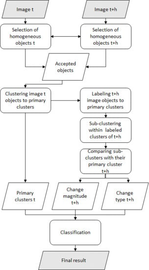
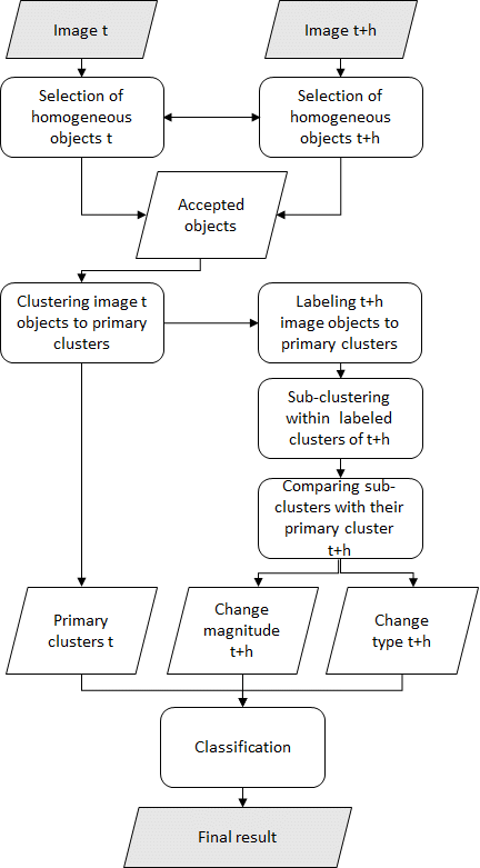
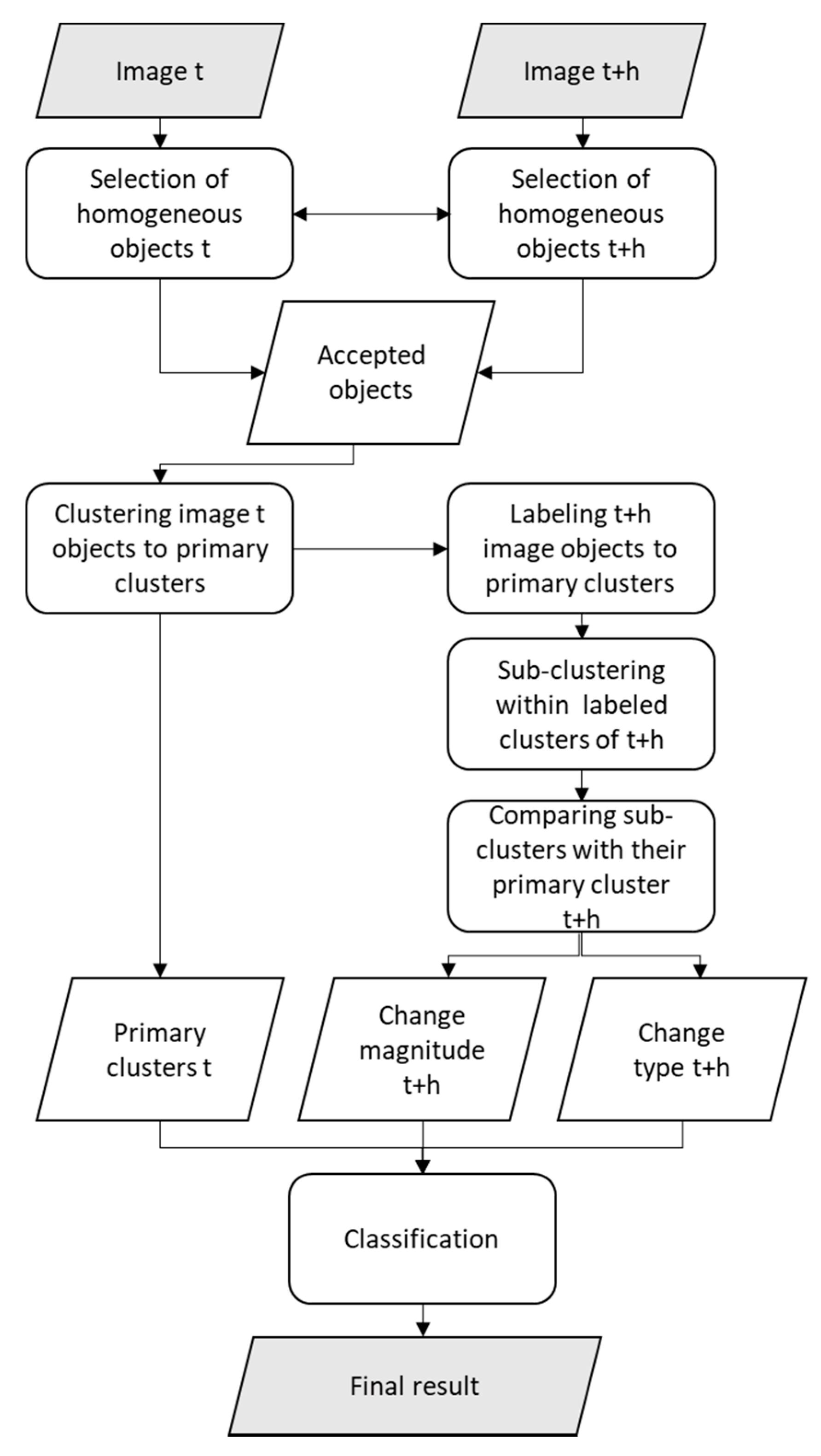
2. Algorithm
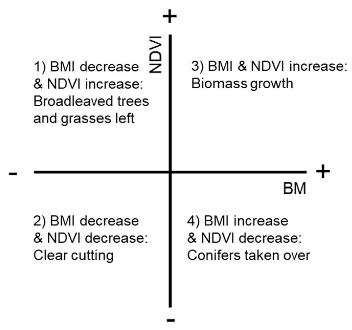
2.1. Computation of Change Features
- BM decrease (red increase) & NDVI increase: can indicate, e.g., conifer tree removal with remaining broad-leaved trees and grasses
- BM decrease & NDVI decrease: typical change due to clear-cuts
- BM increase & NDVI increase: biomass growth
- BM increase & NDVI decrease: biomass growth with associated decrease in broadleaved trees or shrubs and grasses. Such change can be associated with silvicultural operations on conifer regeneration sites, for instance.
- Primary cluster mean intensity vector from the pre-change image;
- Primary and secondary cluster mean intensity vectors from the post-change image, enabling computation of change magnitude;
- Primary and secondary cluster BM and NDVI means from the post-change image, enabling computation of change type.
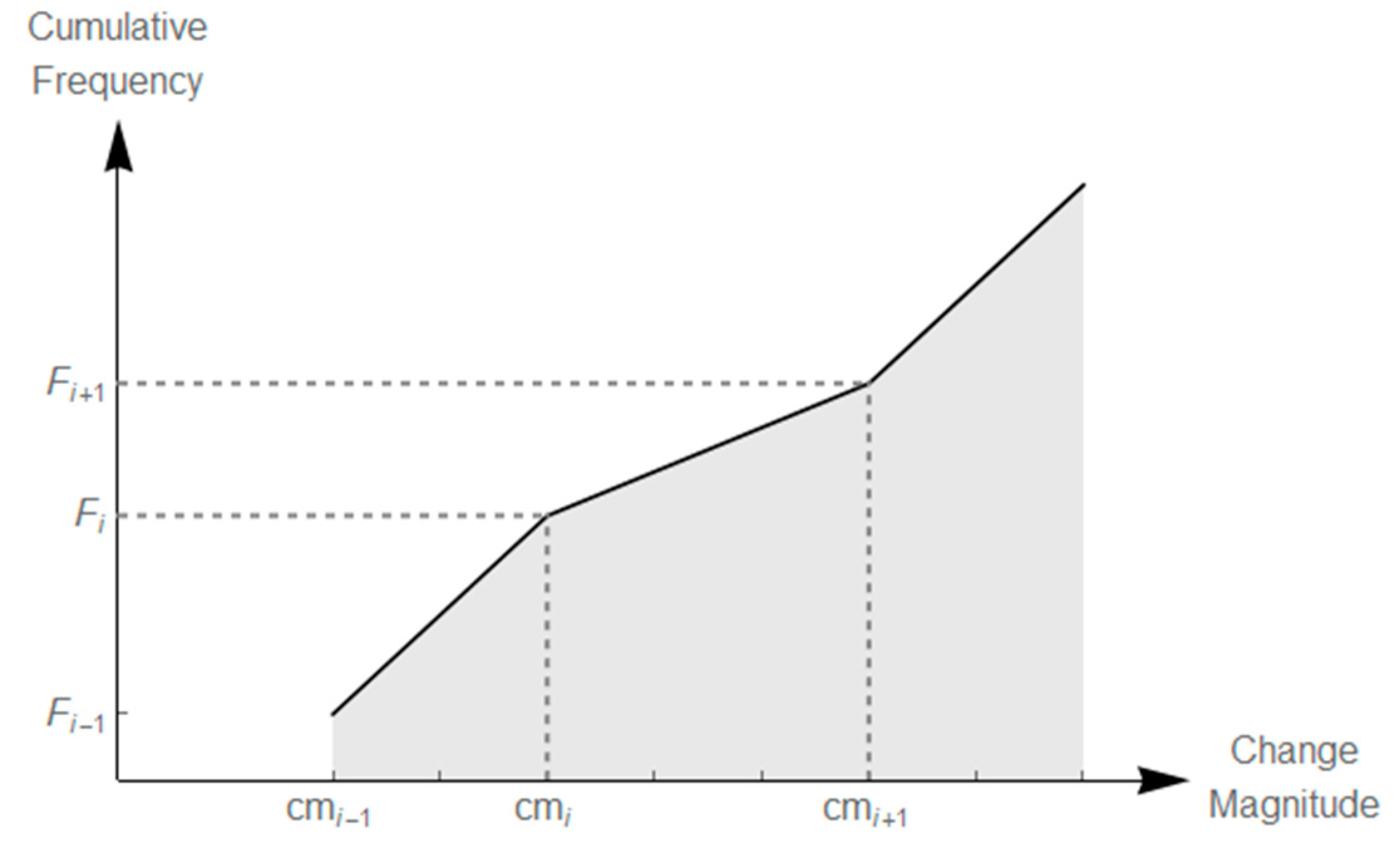
2.2. Compilation of Change Classification Output
- Select the subset of pairs where .
- Sort these pairs according to the values of .
- Discard the pairs in which the values are larger than the 25th percentile of all values within . This reduces the number of pairs to ¼ of the original pairs.
- Sort the remaining pairs according to the values of and output their respective values.
- Select the threshold value among the n lowest slope values. The selection of the threshold from the candidates depends on whether avoiding commission or omission error is more desirable or if it is most important to aim at equal magnitudes of the error types.
3. Demonstration of the Algorithm
3.1. Data
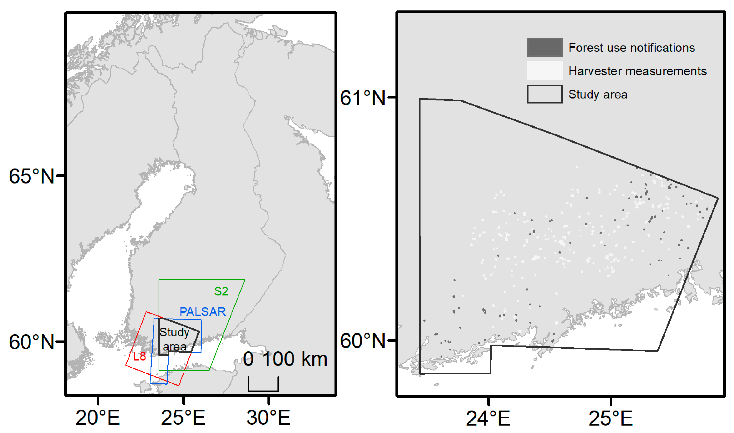
3.1.1. Study Area
3.1.2. Satellite Imagery
3.1.3. Reference Data
3.1.4. Running the Demonstration with Autochange Software
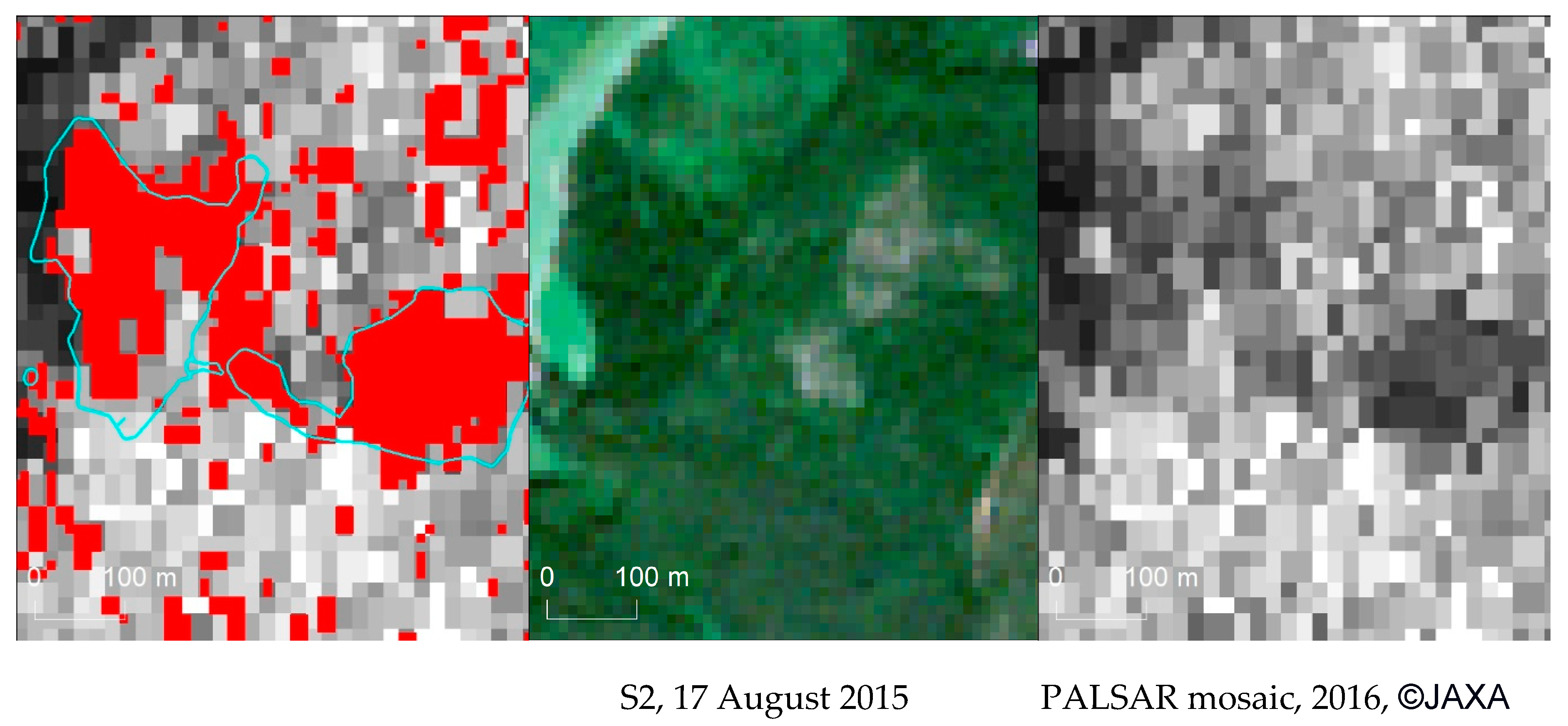
3.1.5. Test with ALOS2 PALSAR
3.2. Results
4. Discussion
5. Conclusions and Future Development Needs
Author Contributions
Funding
Acknowledgments
Conflicts of Interest
References
- European Space Agency Sentinel-2 - Missions - Sentinel Online. Available online: https://sentinels.copernicus.eu/web/sentinel/missions/sentinel-2 (accessed on 2 October 2017).
- Vittek, M.; Brink, A.; Donnay, F.; Simonetti, D.; Desclée, B. Land cover change monitoring using landsat MSS/TM satellite image data over west Africa between 1975 and 1990. Remote Sens. 2013, 6, 658–676. [Google Scholar] [CrossRef]
- Hansen, M.C.; Potapov, P.V.; Moore, R.; Hancher, M.; Turubanova, S.A.; Tyukavina, A.; Thau, D.; Stehman, S.V.; Goetz, S.J.; Loveland, T.R.; et al. High-Resolution Global Maps of 21st-Century Forest Cover Change. Science 2013, 342, 850–853. [Google Scholar] [CrossRef] [PubMed]
- Rullan-Silva, C.D.; Olthoff, A.E.; Delgado de la Mata, J.A.; Pajares-Alonso, J.A. Remote Monitoring of Forest Insect Defoliation–A Review. For. Syst. 2013, 22, 377. [Google Scholar] [CrossRef]
- Häme, T. Spectral interpretation of changes in forest using satellite scanner images. Acta For. Fenn. 1991, 0. [Google Scholar] [CrossRef]
- Matricardi, E.A.T.; Skole, D.L.; Pedlowski, M.A.; Chomentowski, W.; Fernandes, L.C. Assessment of tropical forest degradation by selective logging and fire using Landsat imagery. Remote Sens. Environ. 2010, 114, 1117–1129. [Google Scholar] [CrossRef]
- Achard, F.; Beuchle, R.; Mayaux, P.; Stibig, H.-J.; Bodart, C.; Brink, A.; Carboni, S.; Desclée, B.; Donnay, F.; Eva, H.D.; et al. Determination of tropical deforestation rates and related carbon losses from 1990 to 2010. Glob. Chang. Biol. 2014, 20, 2540–2554. [Google Scholar] [CrossRef]
- Sunar, F.; Özkan, C. Forest fire analysis with remote sensing data. Int. J. Remote Sens. 2001, 22, 2265–2277. [Google Scholar] [CrossRef]
- Kelhä, V.; Rauste, Y.; Häme, T.; Sephton, T.; Buongiorno, A.; Frauenberger, O.; Soini, K.; VenäLäinen, A.; Miguel-Ayanz, J.S.; Vainio, T. Combining AVHRR and ATSR satellite sensor data for operational boreal forest fire detection. Int. J. Remote Sens. 2003, 24, 1691–1708. [Google Scholar] [CrossRef]
- Meng, R.; Dennison, P.E.; Huang, C.; Moritz, M.A.; D ’antonio, C. Effects of fire severity and post-fire climate on short-term vegetation recovery of mixed-conifer and red fir forests in the Sierra Nevada Mountains of California. Remote Sens. Environ. 2015, 171, 311–325. [Google Scholar] [CrossRef]
- Huang, X.; Wen, D.; Li, J.; Qin, R. Multi-level monitoring of subtle urban changes for the megacities of China using high-resolution multi-view satellite imagery. Remote Sens. Environ. 2017, 196, 56–75. [Google Scholar] [CrossRef]
- Li, S.; Sun, D.; Goldberg, M.D.; Sjoberg, B.; Santek, D.; Hoffman, J.P.; DeWeese, M.; Restrepo, P.; Lindsey, S.; Holloway, E. Automatic near real-time flood detection using Suomi-NPP/VIIRS data. Remote Sens. Environ. 2017. [CrossRef]
- Redo, D.J.; Millington, A.C. A hybrid approach to mapping land-use modification and land-cover transition from MODIS time-series data: A case study from the Bolivian seasonal tropics. Remote Sens. Environ. 2011, 115, 353–372. [Google Scholar] [CrossRef]
- PRODES—Coordenação-Geral de Observação da Terra. Available online: http://www.obt.inpe.br/OBT/assuntos/programas/amazonia/prodes (accessed on 30 January 2018).
- McRoberts, R.E. Post-classification approaches to estimating change in forest area using remotely sensed auxiliary data. Remote Sens. Environ. 2014, 151, 149–156. [Google Scholar] [CrossRef]
- IPCC 2006; Eggleston, H.S.; Buendia, L.; Miwa, K.; Ngara, T.; Tanabe, K. (Eds.) 2006 IPCC Guidelines for National Greenhouse Gas Inventories; Volume 4 Agriculture, Forestry and Other Land Use; Institute for Global Environmental Strategies: Hayama, Kanagawa, Japan, 2006. [Google Scholar]
- Deng, J.S.; Wang, K.; Deng, Y.H.; Qi, G.J. PCA-based land-use change detection and analysis using multitemporal and multisensor satellite data. Int. J. Remote Sens. 2008, 29, 4823–4838. [Google Scholar] [CrossRef]
- Green, K.; Kempka, D.; Lackey, L. Using Remote Sensing to Detect and Monitor Land-Cover and Land-Use Ghange. Photogramm. Eng. Remote Sens. 1994, 60, 331–337. [Google Scholar]
- Coppin, P.; Jonckheere, I.; Nackaerts, K.; Muys, B.; Lambin, E. Digital change detection methods in ecosystem monitoring: A review. Int. J. Remote Sens. 2004, 25, 1565–1596. [Google Scholar] [CrossRef]
- Zhu, Z.; Woodcock, C.E. Continuous change detection and classification of land cover using all available Landsat data. Remote Sens. Environ. 2014, 144, 152–171. [Google Scholar] [CrossRef]
- Reiche, J.; de Bruin, S.; Hoekman, D.; Verbesselt, J.; Herold, M. A Bayesian Approach to Combine Landsat and ALOS PALSAR Time Series for Near Real-Time Deforestation Detection. Remote Sens. 2015, 7, 4973–4996. [Google Scholar] [CrossRef]
- Luppino, L.T.; Anfinsen, S.N.; Moser, G.; Jenssen, R.; Bianchi, F.M.; Serpico, S.; Mercier, G. A clustering approach to heterogeneous change detection. In Proceedings of the Scandinavian Conference on Image Analysis, Tromsø, Norway, 12–14 June 2017. [Google Scholar]
- Tewkesbury, A.P.; Comber, A.J.; Tate, N.J.; Lamb, A.; Fisher, P.F. A critical synthesis of remotely sensed optical image change detection techniques. Remote Sens. Environ. 2015, 160, 1–14. [Google Scholar] [CrossRef]
- Collins, J.B.; Woodcock, C.E. An assessment of several linear change detection techniques for mapping forest mortality using multitemporal landsat TM data. Remote Sens. Environ. 1996, 56, 66–77. [Google Scholar] [CrossRef]
- Cartus, O.; Kellndorfer, J.; Walker, W.; Franco, C.; Bishop, J.; Santos, L.; Fuentes, J.M.M. A national, detailed map of forest aboveground carbon stocks in Mexico. Remote Sens. 2014, 6, 5559–5588. [Google Scholar] [CrossRef]
- Nielsen, A.A.; Conradsen, K.; Simpson, J.J. Multivariate Alteration Detection (MAD) and MAF Postprocessing in Multispectral, Bitemporal Image Data: New Approaches to Change Detection Studies. Remote Sens. Environ. 1998, 64, 1–19. [Google Scholar] [CrossRef]
- Jönsson, P.; Eklundh, L. TIMESAT—A program for analyzing time-series of satellite sensor data. Comput. Geosci. 2004, 30, 833–845. [Google Scholar] [CrossRef]
- Verbesselt, J.; Hyndman, R.; Newnham, G.; Culvenor, D. Detecting trend and seasonal changes in satellite image time series. Remote Sens. Environ. 2010, 114, 106–115. [Google Scholar] [CrossRef]
- Kennedy, R.E.; Yang, Z.; Cohen, W.B. Detecting trends in forest disturbance and recovery using yearly Landsat time series: 1. LandTrendr—Temporal segmentation algorithms. Remote Sens. Environ. 2010, 114, 2897–2910. [Google Scholar] [CrossRef]
- Zhu, Z. Change detection using landsat time series: A review of frequencies, preprocessing, algorithms, and applications. ISPRS J. Photogramm. Remote Sens. 2017, 130, 370–384. [Google Scholar]
- Zhu, Z.; Zhang, J.; Yang, Z.; Aljaddani, A.H.; Cohen, W.B.; Qiu, S.; Zhou, C. Continuous monitoring of land disturbance based on Landsat time series. Remote Sens. Environ. 2019. [CrossRef]
- Reiche, J.; Hamunyela, E.; Verbesselt, J.; Hoekman, D.; Herold, M. Improving near-real time deforestation monitoring in tropical dry forests by combining dense Sentinel-1 time series with Landsat and ALOS-2 PALSAR-2. Remote Sens. Environ. 2018, 204, 147–161. [Google Scholar] [CrossRef]
- Häme, T.; Heiler, I.; San Miguel-Ayanz, J. An unsupervised change detection and recognition system for forestry. Int. J. Remote Sens. 1998, 19. [Google Scholar] [CrossRef]
- Pitkänen, T.P.; Sirro, L.; Häme, L.; Häme, T.; Törmä, M.; Kangas, A. Errors related to the automatized satellite-based change detection of boreal forests in Finland. Int. J. Appl. Earth Obs. Geoinf. 2020, 86, 102011. [Google Scholar] [CrossRef]
- National Research Council. Remote Sensing with Special Reference to Agriculture and Forestry; The National Academies Press: Cambridge, MA, USA, 1970; ISBN 978-0-309-01723-7. [Google Scholar]
- Häme, T. Interpretation of deciduous trees and shrubs in conifer seedling stands from Landsat imagery. Photogramm. J. Finl. 1984, 9, 209–217. [Google Scholar]
- Finnish Statistical Yearbook of Forestry 2014; Peltola, A., Ed.; Metsäntutkimuslaitos, Vantaan toimipaikka: Tampere, Finland, 2014; ISBN 978-951-40-2505-1. [Google Scholar]
- Vaahtera, E.; Aarne, M.; Ihalainen, A.; Mäki-Simola, E.; Peltola, A.; Torvelainen, J.; Uotila, E.; Ylitalo, E. (Eds.) Finnish Frest Statistics; Luke: Helsinki, Finland, 2018; ISBN 978-952-326-701-5. [Google Scholar]
- Parmes, E.; Rauste, Y.; Molinier, M.; Andersson, K.; Seitsonen, L.; Parmes, E.; Rauste, Y.; Molinier, M.; Andersson, K.; Seitsonen, L. Automatic Cloud and Shadow Detection in Optical Satellite Imagery Without Using Thermal Bands—Application to Suomi NPP VIIRS Images over Fennoscandia. Remote Sens. 2017, 9, 806. [Google Scholar] [CrossRef]
- Shimada, M.; Itoh, T.; Motooka, T.; Watanabe, M.; Shiraishi, T.; Thapa, R.; Lucas, R. New global forest/non-forest maps from ALOS PALSAR data (2007-2010). Remote Sens. Environ. 2014, 155, 13–31. [Google Scholar] [CrossRef]
- Guns, R.; Lioma, C.; Larsen, B. The tipping point: F-score as a function of the number of retrieved items. Inf. Process. Manag. 2012, 48, 1171–1180. [Google Scholar] [CrossRef]
- Melkas, T.; Riekki, K.; Sorsa, J.-A. Automated Stand Delineation Based on Harvester Location Data Metsätehon tuloskalvosarja 7b/2018 Timo Melkas; Metsäteho: Vantaa, Finland, 2018. [Google Scholar]
- Molinier, M.; Astola, H.; Raty, T.; Woodcock, C. Timely And Semi-Automatic Detection of Forest Logging Events in Boreal Forest Using All Available Landsat Data. In Proceedings of the IGARSS 2018—2018 IEEE International Geoscience and Remote Sensing Symposium, Valencia, Spain, 23–27 July 2018; pp. 1730–1733. [Google Scholar]
- Baetens, L.; Desjardins, C.; Hagolle, O. Validation of Copernicus Sentinel-2 Cloud Masks Obtained from MAJA, Sen2Cor, and FMask Processors Using Reference Cloud Masks Generated with a Supervised Active Learning Procedure. Remote Sens. 2019, 11, 433. [Google Scholar] [CrossRef]
- Lucas, R.; Armston, J.; Fairfax, R.; Fensham, R.; Accad, A.; Carreiras, J.; Kelley, J.; Bunting, P.; Clewley, D.; Bray, S.; et al. An Evaluation of the ALOS PALSAR L-Band Backscatter—Above Ground Biomass Relationship Queensland, Australia: Impacts of Surface Moisture Condition and Vegetation Structure. IEEE J. Sel. Top. Appl. Earth Obs. Remote Sens. 2010, 3, 576–593. [Google Scholar] [CrossRef]
- Häme, T.; Tergujeff, R.; Rauste, Y.; Farquhar, C.; van Zetten, P.; Kershaw, P.; de Groof, A.; Hämäläinen, J.; van Bemmelen, J.; Seifert, F.M. Forestry-TEP responds to user needs for sentinel data value adding in cloud. In Proceedings of the Conference on Big Data from Space, BiDS’2017, Toulouse, France, 28–30 November 2017; pp. 239–242. [Google Scholar] [CrossRef]


| Change Class | Number of Stands | Minimum Area (ha) | Median Area (ha) | Maximum Area (ha) |
|---|---|---|---|---|
| Clear-cut | 141 * | 0.5 | 1.8 | 12.2 |
| Uncut | 6 * 1825 ** | 0.5 | 1.8 | 41.0 |
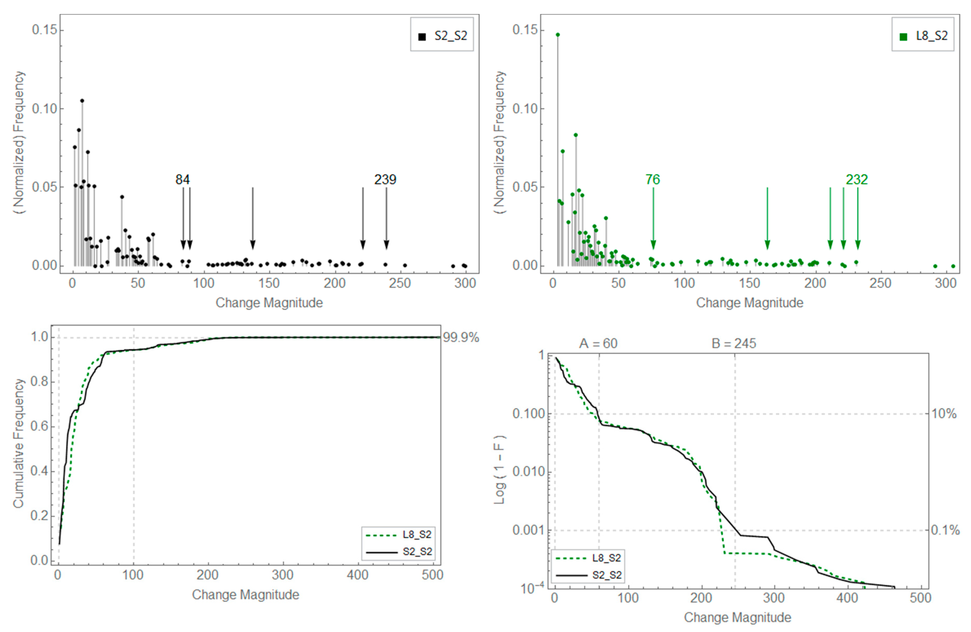
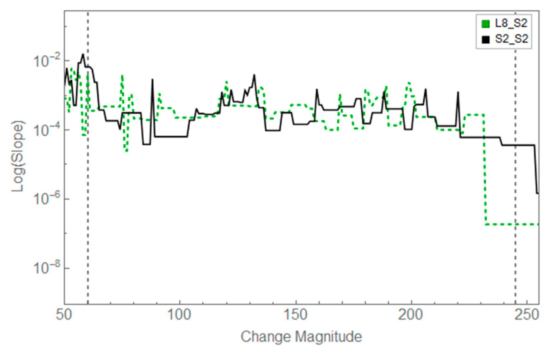
| Image Pair | 1 | 2 | 3 | 4 | 5 |
|---|---|---|---|---|---|
| S2-S2 | 84 | 89 | 137 | 221 | 239 |
| L8-S2 | 76 | 163 | 211 | 221 | 232 |
| Prediction | Reference | ||
|---|---|---|---|
| Un-cut | Clear-cut | Total | |
| Uncut (50%) | 1817 (1810) | 8 (15) | 1825 |
| Clear-cut (50%) | 7 (17) | 136 (126) | 143 |
| Total | 1824 (1827) | 144 (141) | 1968 |
| Overall agreement % | 99.2 | ||
| OE for cut class % | 5.6 | ||
| OE for uncut class % | 0.4 | ||
| CE for cut class % | 4.9 | ||
| CE for uncut class % | 0.4 | ||
| F1 score for cut class % | 94.8 | ||
| Prediction | Reference | ||
|---|---|---|---|
| Un-cut | Clear-cut | Total | |
| Uncut (50%) | 1820 (1815) | 30 (35) | 1850 |
| Clear-cut (50%) | 4 (12) | 114 (106) | 118 |
| Total | 1824 (1827) | 144 (141) | 1968 |
| Overall agreement % | 98.3 | ||
| OE for cut class % | 20.8 | ||
| OE for uncut class % | 0.2 | ||
| CE for cut class % | 3.4 | ||
| CE for uncut class % | 0.2 | ||
| F1 score for cut class % | 87.0 | ||
| Prediction | Reference | ||
|---|---|---|---|
| Un-cut | Clear-cut | Total | |
| Uncut (50%) | 1798 (1791) | 24 (31) | 1822 |
| Clear-cut (50%) | 26 (36) | 120 (110) | 146 |
| Total | 1824 (1827) | 144 (141) | 1968 |
| Overall agreement % | 97.5 | ||
| OE for cut class % | 16.7 | ||
| OE for uncut class % | 1.4 | ||
| CE for cut class % | 17.8 | ||
| CE for uncut class % | 1.3 | ||
| F1 score for cut class % | 82.8 | ||
© 2020 by the authors. Licensee MDPI, Basel, Switzerland. This article is an open access article distributed under the terms and conditions of the Creative Commons Attribution (CC BY) license (http://creativecommons.org/licenses/by/4.0/).
Share and Cite
Häme, T.; Sirro, L.; Kilpi, J.; Seitsonen, L.; Andersson, K.; Melkas, T. A Hierarchical Clustering Method for Land Cover Change Detection and Identification. Remote Sens. 2020, 12, 1751. https://doi.org/10.3390/rs12111751
Häme T, Sirro L, Kilpi J, Seitsonen L, Andersson K, Melkas T. A Hierarchical Clustering Method for Land Cover Change Detection and Identification. Remote Sensing. 2020; 12(11):1751. https://doi.org/10.3390/rs12111751
Chicago/Turabian StyleHäme, Tuomas, Laura Sirro, Jorma Kilpi, Lauri Seitsonen, Kaj Andersson, and Timo Melkas. 2020. "A Hierarchical Clustering Method for Land Cover Change Detection and Identification" Remote Sensing 12, no. 11: 1751. https://doi.org/10.3390/rs12111751
APA StyleHäme, T., Sirro, L., Kilpi, J., Seitsonen, L., Andersson, K., & Melkas, T. (2020). A Hierarchical Clustering Method for Land Cover Change Detection and Identification. Remote Sensing, 12(11), 1751. https://doi.org/10.3390/rs12111751