Abstract
Remote-sensing tools and satellite data are often used to map and monitor changes in vegetation cover in forests and other perennial woody vegetation. Large-scale vegetation mapping from remote sensing is usually based on the classification of its spectral properties by means of spectral Vegetation Indices (VIs) and a set of rules that define the connection between them and vegetation cover. However, observations show that, across a gradient of precipitation, similar values of VI can be found for different levels of vegetation cover as a result of concurrent changes in the leaf density (Leaf Area Index—LAI) of plant canopies. Here we examine the three-way link between precipitation, vegetation cover, and LAI, with a focus on the dry range of precipitation in semi-arid to dry sub-humid zones, and propose a new and simple approach to delineate woody vegetation in these regions. By showing that the range of values of Normalized Difference Vegetation Index (NDVI) that represent woody vegetation changes along a gradient of precipitation, we propose a data-based dynamic lower threshold of NDVI that can be used to delineate woody vegetation from non-vegetated areas. This lower threshold changes with mean annual precipitation, ranging from less than 0.1 in semi-arid areas, to over 0.25 in mesic Mediterranean area. Validation results show that this precipitation-sensitive dynamic threshold provides a more accurate delineation of forests and other woody vegetation across the precipitation gradient, compared to the traditional constant threshold approach.
1. Introduction
Remote-sensing tools are widely used to map different attributes of vegetation at various spatial scales [1,2]. Precise vegetation mapping is a first and vital step for long-term monitoring of vegetation dynamics [3], in particular for long-living plants such as trees and shrubs in several woody vegetation systems, in which different environmental effects influence the observed temporal trends.
One of the commonly used tools for vegetation monitoring is satellite data, which allow continuous observation of vegetation at sufficient spatial and temporal resolutions and constant return frequencies. Another advantage of satellite data for temporal analysis is that it can now be retrieved from a single sensor, therefore allowing analysis across long time series with no further calibration.
Aerial photography is also widely used to map vegetation cover, often at spatial resolutions that are considerably better compared to satellite-derived data. However, aerial photography is less useful for long-term monitoring or large-scale mapping because of non-uniformity in the imaging methods, including the use of different sensors, different resolutions, inconsistent return frequencies, and different calibration procedures.
Vegetation indices (VI), such as the Normalized Difference Vegetation Index (NDVI) [4], are frequently used for vegetation monitoring and mapping, in particular for individual tree delineation. Several methods are widely used for vegetation delineation: supervised classification (e.g., [5]), spectral methods (e.g., [6]), and machine-learning algorithms [7], or a simple constant lower threshold value (e.g., [8]).
Vegetation mapping methods, such as classification, spectral unmixing and machine learning require large datasets for training, and require much computing power and time compared to the simple threshold approach and, therefore, are less efficient for large-scale mapping and long-term monitoring. For example, the global tree cover dataset developed by Hansen et al. [3] within the Google infrastructure is widely used for temporal analysis of forest gain/loss. The training and validation datasets for this global tree cover map are based on data of forests in the main types of humid biomes (temperate, Boreal and tropical) but lack data from forests in drier regions. Therefore, this dataset can lead to false-negative detection of forest in dry biomes.
The constant threshold approach defines a minimum constant value of NDVI (or other VI) that assumes no vegetation at values below this threshold, regardless of geographic location or environmental conditions [8,9,10]. This lower threshold NDVI value is usually 0.2, while NDVI values of 0.2 < NDVI < 1 are assumed to be positively (although not necessarily linearly) correlated with vegetation cover [9]. This lower threshold of NDVI was found useful for forest mapping, in particular in mesic environments with high precipitation load.
However, observations show large difference in the values of NDVI obtained for similar values of vegetation cover, when comparing across regions with different levels of precipitation [11]. Such differences can result in under-detection of forests, especially in regions with low precipitation load. Therefore, here we argue that the constant threshold approach is not sensitive enough for precise long-term analyses, because it results in large false-negative errors when mapping woody vegetation in dry regions (with arid, semi-arid, and even Mediterranean climate) and false-positive errors in humid regions. Furthermore, NDVI values cannot provide sufficient information about changes in the structure of woody vegetation (e.g., changes in the area covered by vegetation vs. the internal structure of leaf area and leaf density of this vegetation) which can result in false delineation when comparing across sites with widely different precipitation amounts. Moreover, changes in the NDVI value in the same location between two time steps might be interpreted either as change in vegetation cover or biomass.
In general, we know that leaf mass and leaf area of plants are both tightly related to hydrological budget and water use by plants [12]. Woodward [13] showed that this budget can be used to predict the maximum Leaf Area Index (LAI) of woody plants, i.e., the total one-sided area of leaf tissue per unit ground surface area (m2 × m−2; [14]). Kahiu and Hanan [15] found a strong empirical correlation between MODIS retrievals of the LAI and mean annual precipitation (MAP). In situ measurements of LAI also showed high correlation to MAP [16].
However, it is worth noting some differences in the definition of vegetation cover and LAI between the remote-sensing perspective and the field-ecological perspective. From the ecological perspective, an increase in the availability of water to plants can result in increasing LAI within an area of vegetation cover, which accordingly can result in an increase in NDVI with no change in vegetation cover in the pixel. Alternatively, NDVI can increase as a result of increasing vegetation cover with similar LAI, or a combination of increases in both cover and LAI. LAI derived from remotely sensed data is usually based on parametrization of the Fractional Vegetation Cover (FVC). Therefore, from the remote-sensing perspective it is difficult to distinguish between the two causes of change, although in many cases increasing inputs of precipitation will be associated with an increase in both vegetation cover, plant biomass, and LAI [11,17].
We, therefore, performed a qualitative analysis that illustrates the limitations of using VIs to monitor and interpret changes in vegetation cover and biomass. To overcome these limitations, we developed a new simple method for woody vegetation delineation using a dynamic NDVI threshold as a function of MAP, based on a training set of NDVI and vegetation covers.
2. Materials and Methods
2.1. Data
Sentinel 2. Sentinel-2 is a wide-swath, high-resolution (10 m), multi-spectral imaging mission supporting Copernicus Land Monitoring studies, including the monitoring of vegetation, soil, and water cover, as well as observation of inland waterways and coastal areas. The atmospherically corrected product, Level 2A [18], was used within the Google Earth Engine environment [19]. Following Roderick et al. [20], we assume that in regions with a long dry summer the NDVI signal at the end of the summer is contributed from woody vegetation only, excluding all ephemeral herbaceous vegetation. We searched for images acquired over Israel at the end of the dry season (mid-August to end of September; [21]) with minimum cloud cover using mask cloud probability field from level 2A product [18].
Woody vegetation cover dataset over Israel. Data on the FVC of woody vegetation in Israel was obtained from the 10 m spatial resolution Israeli wide Fractional Vegetation Cover product [22], which matches the spatial resolution of Sentinel-2 products. This product was derived from the nation-wide orthophoto at 0.5 m spatial resolution obtained at the end of the summer.
First, each pixel in the orthophoto was classified as woody or non-woody using two methods: (1) color quantization and (2) chromatic green threshold (chromatic green= green/(red+green+blue)). Then, the FVC was defined as the ratio of woody to non-woody pixels at the 10 m scale (400 pixels), similar to the spatial resolution of Sentinel-2 products.
Land cover and land use (LCLU) over Israel. The LCLU product was obtained from the HaMaarag—Israel’s National Ecosystem Assessment Program. This dataset is based on numerus vector and raster datasets with a resolution of 25 m [23].
Validation dataset. The entire study region in Israel was stratified to 16 classes of 50 mm of MAP, ranging between 200 and 1000 mm yr−1. For each class, 500 points were randomly selected, with a total of 8000 points throughout Israel. Each point was related to the containing pixel in the S2 product. To prepare this validation dataset, we used a recent aerial orthophoto of Israel (at a resolution of 0.5 m) from which we manually classified the presence/absence of woody vegetation and the type of vegetation cover in all randomly selected pixels. Pixels that contained woody vegetation were classified into three categories: shrubs, forest trees (referring to planted forests), and woodland trees (see below).
2.2. Methods
Study area. We focused our analyses on the semi-arid and Mediterranean climate regions in Israel. The MAP in these regions ranges between a mean annual precipitation of ~150 mm/y to ~900 mm/y in the humid Mediterranean regions at the northern edge, with large inter-annual variability [24]. The rainy season throughout Israel is very short, concentrated between October and May, with most rainfall occurring in December, January, and February (ca. 60% of the annual amount). The woody vegetation in the area includes: shrublands with shrubs of different sizes (ranging 0.5–2 m height), woodlands with intermixed tree and shrubs, and planted forests composed mainly of trees that usually are more uniform in structure and composition. Trees and shrubs in these woody vegetation systems are spatially spread at different densities, resulting in different levels of vegetation cover.
Theoretical analysis of NDVI as a function of changing LAI and FVC. We used the PROSAIL model to simulate canopy spectra and to calculate the expected value of NDVI obtained as a function of defined values of LAI and vegetation cover. PROSAIL is a canopy radiative transfer scheme that couples the leaf (PROSPECT) and canopy (4-SAIL) radiative transfer models [25]. We simulated tree canopy spectra with LAI ranging from 0.2 to 2, representing a low range of LAI values that are harder to delineate. To calculate the expected NDVI of vegetation in a pixel containing both vegetation and the surrounding areas of soil that is not covered by vegetation, these spectra (S) were linearly mixed with the soil spectra using FVC as a weighting coefficient, as follows:
where “Tree” is the typical spectra of the woody vegetation and “Soil” is the typical spectra of limestone, representing the most common type of soil material over Israel, This is important because different soil types also influence the spectral signal from a pixel, especially in dry areas in which FVC tends to be small and much of the area within each land pixel can be covered by bare soil and not woody vegetation.
S = Tree·FVC + Soil·(1 − FVC)
Finally, the NDVI was calculated for each pixel from the simulated spectra. It is important to notice that the 4-SAIL model parametrizes the FVC as function of LAI. For example, low LAI will lead to high FVC. In this analysis we ignored this feature of the model and used a simple spectral mixing instead.
Calibrating a dynamic NDVI threshold and range across a gradient of precipitation. To calibrate the NDVI threshold, we calculated SENTINEL 2-based NDVI for 50,000 randomly selected pixels using the Google Earth Engine (GEE) covering all land-cover classes from the classes in the HaMaarag LCLU product. From these pixels, we selected only pixels defined as covering natural vegetated areas, which were further divided into two categories of woody and non-woody vegetation. Categorization into woody and non-woody was based on the following method: from the land-cover layer we selected only the pixels of three main woody vegetation cover types: shrubs, planted forest trees, and woodland trees. We used the woody vegetation cover dataset to omit all pixels with a low vegetation cover, less than 10%, to avoid overestimation of woody cover where this cover is negligible.
Mean annual precipitation for each pixel was defined using a MAP dataset of the Israeli Meteorological Service at 500 m spatial resolution. All points were binned into 50 mm yr−1 bins according to the resolution of the MAP data, therefore providing estimates of the change along the precipitation gradient.
We analyzed the NDVI value of all pixels as a function of the binned MAP. For each precipitation bin in the range of 200–900 mm yr−1 (precipitation gradient for afforestation in Israel) we analyzed the distribution of NDVI and looked for the 1st, 5th, 10th, median, 90th, and 95th quantiles. Curves for the upper and lower thresholds of NDVI were fitted as a function of precipitation using the 10th and 95th quantiles for the tree cover data. We used the lower curve (based on the 10th quantile) as a precipitation-sensitive dynamic threshold for woody vegetation delineation. The upper threshold (based on the 95th quantile analysis) can be used to estimate FVC by scaling each NDVI value in the range between minimum and maximum NDVI values in each precipitation bin in our analysis. We repeated these analyses for all the data combined, and separately for two categories of woody cover type (shrubs vs. trees; the latter includes both forests and woodlands).
Testing sensitivity to spatial resolution and scale. Since NDVI and FVC are scale-dependent [26], and vegetation cover in drylands is usually sparse, the chance of finding pixels without any vegetation or with high FVC is strongly influenced by the spatial resolution of the analysis. Accordingly, we tested whether the scale of the analysis influences the threshold calibration. To test the influence of the spatial resolution on the dynamic threshold of the NDVI-MAP curve we compared the dynamic threshold curves derived in a similar manner from Landsat 8 (30 m pixel resolution) and from Sentinel-2 (10 m pixel resolution).
Validation. The precipitation-sensitive threshold approach was implemented to detect woody vegetation over the entire study area, using NDVI values of the SENTINEL-2 2A product from 28th September, 2018.
Using the long-term MAP data, we calculated the dynamic threshold for corresponding precipitation values for each pixel, and checked whether the NDVI value was above or below the dynamic threshold. All pixels with an NDVI above the dynamic threshold were defined as containing woody vegetation. We validated the accuracy of the automatic classification using the manually classified validation dataset (see validation dataset above), by comparing the agreement among pixels classified into two categories: woody vegetation cover and non-woody vegetation cover, and calculated the Accuracy and Kappa values.
Evaluation of the new method in a different region. We tested our new precipitation-sensitive threshold method to detect woody vegetation cover in different locations in Israel and in a dry region with a similar Mediterranean-type climate (characterized by a warm rainless summer) in Spain (Murcia region). We compare the detection with our precipitation-sensitive threshold method to classification of the woody vegetation using two other common methods: a constant threshold of NDVI ≥ 0.2, and the tree cover dataset implemented on the GEE [3].
3. Results
The PROSAIL model analysis shows that changes in NDVI are sensitive to the combination of LAI (Figure 1a) and FVC (Figure 1b) meaning that the same NDVI value can represent various scenarios of vegetation cover due to interaction between vegetation cover and LAI. The combined effect of vegetation cover and LAI is most pronounced when NDVI values range between 0.2 and 0.7 (see in Figure 1 many lines with a similar NDVI value resulting from different combinations of LAI and FVC). The analysis also shows a suite of woody vegetation cover scenarios with NDVI values <0.2, when FVC is smaller than 0.33 or when FVC is high, but the leaf area of the vegetative cover is sparse (e.g., LAI < 0.5). This analysis therefore presents the caveat of the constant threshold of NDVI for vegetation delineation.
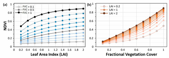
Figure 1.
Changes in the Normalized Difference Vegetation Index (NDVI) as a function of increasing Fractional Vegetation Cover (FVC) and Leaf Area Index (LAI): (a) NDVI values per pixel with increasing LAI per unit area of vegetation cover, for different FVC levels within the pixel (light to dark colors); (b) NDVI values per pixel with increasing FVC within the pixel, for different level of LAI per unit area of vegetation cover (light to dark colors).
Our analysis of the distribution of NDVI values along the precipitation gradient in Israel shows that both the lower and upper thresholds of NDVI increase as a function of MAP. The patterns of increase, however, are different between the two thresholds (Figure 2). Figure 2a shows that the lower threshold, indicating the lowest value of NDVI at which we expect to find shrubs, ranges from less than 0.1 in the dry end of the precipitation gradient (200 mm yr−1) to more than 0.2 in the wet end of the gradient (>800 mm yr−1), for the 10th quantile of the data. This means that using a constant threshold of 0.2 will lead to either under-detection or false-positive delineation. The upper threshold for shrubs (based on the 95th quantile), indicating the value of NDVI at which we expect to find full woody cover (FVC = 1), ranges from less than 0.4 in the dry end of the gradient to almost 0.8 in the wet end of the gradient.
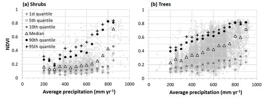
Figure 2.
Changes in the Normalized Difference Vegetation Index (NDVI) of shrub and tree cover along the precipitation gradient. Results of all analyzed pixels for shrub cover (a) and for tree cover (b) are shown in gray. Quantiles for each bin of 50 mm of annual precipitation are shown in greyscale symbols overlying the data.
Figure 2b shows that the lower threshold for trees also ranges from less than 0.2 (~0.15) in the dry end of the precipitation gradient to 0.4 in the wet end of the gradient (900 mm yr−1). The 10th percentile curve was chosen as a robust lower threshold to avoid unique cases in which only a part of a plant is in the training pixel, but have little effect on the S2 product NDVI. The upper threshold of the 95th quantile for trees ranges from 0.45 in the dry end of the precipitation gradient to over 0.8 in the wet end of the gradient.
Figure 2 therefore shows that the curve of the increase of NDVI threshold as a function of precipitation is considerably steeper for the upper threshold compared to the lower threshold. Furthermore, the analysis shows that the conservative lower threshold of NDVI = 0.2 is too high to detect woody vegetation in the low ranges of cover in arid, semi-arid, and Mediterranean biomes, but too low compared to the actual values of NDVI that exist for woody cover in the high range of this precipitation gradient.
Figure 3 shows a comparison of three different mapping methods: Hansen global tree cover (red), constant NDVI threshold (NDVI ≥ 0.2; blue) and our newly proposed dynamic threshold (green) for (a) Yatir forest and (b) Judean mountains. Figure 3a shows that for the Yatir forest, located in a semi-arid environment in the northern Negev Desert, Israel (200 mm annual rainfall) [27], most of the tree cover is not detected by the Hansen tree cover dataset while the constant NDVI threshold and the dynamic threshold capture most of this dry forest. For the shrubland and forest in the Judean mountains, Israel (500 mm annual rainfall) Figure 3b shows a better detection by all three methods compared to the detection success in the semi-arid forest, but with some false-negative forest mapping by the Hansen dataset and even by the constant threshold approach.
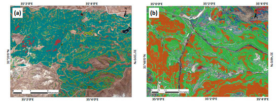
Figure 3.
Examples of automatic mapping of woody vegetation in two regions in Israel: (a) Yatir forest (200 mm year−1), and (b) Judean mountains (500 mm year−1); using the tree cover dataset from Hansen et al. [3] (in red), the minimum 0.2 NDVI threshold (in blue), and our suggested dynamic precipitation-sensitive threshold (in green).
The validation of the new precipitation-sensitive dynamic threshold shows a high accuracy of detection of woody vegetation, and an improved Accuracy and Kappa value compared to the two most common alternative methods (Table 1, Supplementary Tables S1–S3).

Table 1.
Comparison of the validation results of the proposed precipitation-sensitive dynamic threshold method compared to two alternative methods.
Figure 4 shows an example of the use of our precipitation-sensitive dynamic threshold to delineate woody vegetation in a Mediterranean climate region in the Western Mediterranean Basin: near the city of Murcia, Spain. A qualitative comparison of the goodness of delineation shows an improved detection of sparse woody vegetation using the dynamic threshold approach. The dynamic threshold method detected most of the trees and shrubs in the dry regions of Southern Spain, according to our personal visual inspection of the detailed satellite data. Compared to this dynamics threshold, Figure 4 shows much false-negative detection, i.e., under-detection of the woody vegetation, using the two other approaches: the Hansen tree cover dataset and the constant threshold.
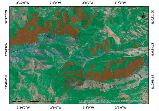
Figure 4.
Example of vegetation delineation in a Mediterranean dryland. Detection of woody cover using three methods: the precipitation-sensitive dynamic threshold algorithm (green), forest mapping dataset by Hansen et al., ([3]; red) and false-positive detection by the constant threshold NDVI of 0.2 (blue).
Figure 5 shows that the shape of upper and lower threshold curves derived from the lower resolution data of Landsat 8 compared to the high-resolution data of Sentinel 2 a very similar, with a small deviation between them. The curves derived from Landsat 8 data are confined within the curves derived from Sentinel-2 data.
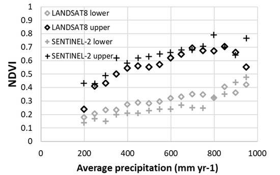
Figure 5.
Comparison of the lower and upper precipitation-sensitive dynamic thresholds at different spatial scales of analysis. Comparison between the lower 10th quantile (gray) and upper 95th quantile (black) thresholds from an analysis of LANDSAT-8 (diamonds) and Sentinel-2 (pluses) products.
4. Discussion
The use of remotely sensed Vegetation Indices, such as NDVI and others, is a common method to delineate and measure vegetation cover. Here we showed that the same value of NDVI can represent different combinations of spatial vegetation cover (FVC), and density of leaves per area covered (LAI), due to the interactive influence of the two factors on the spectral signal at the level of the pixel (Figure 1). Both vegetation cover and LAI are strongly influenced by the growth conditions for the vegetation primarily defined by precipitation, which affects water availability for plants and their hydrological budget. We show that the combination of habitat factors (precipitation or aridity) with vegetation response in terms of FVC and LAI, influence the remotely sensed vegetation index requiring, therefore, special attention, in particular while delineating the vegetation in areas with limited soil water such as drylands.
Our analysis along a wide range of precipitation (200–1000 mm yr−1) showed that a dynamic lower threshold of NDVI, which changes along the precipitation gradient (Figure 2), is more accurate for vegetation delineation compared to other commonly used methods such as the constant threshold of NDVI = 0.2 (Table 1). The dynamic lower threshold of NDVI starts at values <0.2 in semi-arid regions and is exponentially increasing with precipitation to values >0.2 in mesic Mediterranean regions.
The change in the lower threshold is small but significant for a proper detection of woody vegetation in drylands, which together compose around 40% of the terrestrial land globally. These differences between the constant threshold of 0.2 and the actual distribution of vegetation that we found in our analysis explain the false-negative and false-positive delineation of vegetation in dry and wet areas, respectively.
The upper threshold of the vegetation also increased exponentially with increasing precipitation, but we found different shapes for the curves of the lower and upper thresholds (Figure 2). We further show that, as a result of the differences between the curves of the lower and upper thresholds, the range between the two thresholds of NDVI also increases along the precipitation gradient. For each level of precipitation, this range of NDVI values between lower and upper thresholds is related to a gradual increase in vegetation cover, but this increase is not linear with FVC. Additional exploration of the pattern of change in vegetation structure, cover, and density along the NDVI range, would further contribute to improve the use of VIs not only for delineation but also to better characterize the vegetation.
The dynamic precipitation-sensitive threshold approach we propose here is therefore useful to improve the accuracy of vegetation delineation, especially in dry areas with a clear rainless season. This method is applicable for comparison of different areas at the same time, and for temporal monitoring of the year-to-year variability in specific locations. Furthermore, monitoring through time can be used to identify areas of potential vegetation or areas in which vegetation has been strongly disturbed or disappeared (e.g., by monitoring vegetation structure in the past using satellite records).
Two caveats are important to notice here. First, the variability in NDVI values is primarily related to the structure of the vegetation but can also be affected by the spectral properties of the soil. For example: dark soil or soil with biogenic activity can increase NDVI value with no change in vegetation, because of the high reflectance of such soils resulting in a rather high NDVI of some soil types compared to other [28]. The spectral contribution of the signal from the soil will be more pronounced when FVC is small, because of the relatively large area cover of soil (50–90% of the area). A second caveat is due to the well-known saturation of NDVI values at high vegetation covers and LAI that may lead to overestimation of FVC. The typical saturation at NDVI>0.8 [29] is apparent only at the wet end of the precipitation gradient in our analysis. Furthermore, the sensitivity of the threshold analysis to the spatial resolution of the data (Figure 5) shows that the low-resolution threshold (derived from Landsat 8 data) is more confined compared to the threshold derived from the high-resolution data (Sentinel-2). This can be explained by the lower resolution of Landsat data, which lead to lower probability of sampling extreme FVC values.
Verstraete and Pinty [30] argued that for semi-arid regions NDVI is more strongly controlled by changes in vegetation cover than by changes in the optical thickness of canopies. Some evidence for this can be found in the shape of the NDVI threshold curve. The best fit shape of both NDVI thresholds were exponential (Figure 2a,b), resembling the curves of change in NDVI as a function of increasing FVC (Figure 1b), which might suggest that our threshold analysis is primarily driven by changes in vegetation cover along the precipitation gradient in Israel. Data on the LAI of forest trees along the precipitation gradient [16] also shows that the LAI of the trees ranged 0.74 to 2.2 m2 m−2, along a range of 257–722 mm yr−1, but the overall LAI of all vegetation in these stands was correlated with rainfall. Therefore, we suggest that more theoretical and empirical work can provide insights on the interactions and relative contribution of FVC and LAI for the spectral signals of vegetation.
5. Conclusions
This paper introduces a new and simple method for woody vegetation delineation. We used an empirical relation between NDVI and MAP and fitted a curve that can be used as a dynamic threshold for woody vegetation delineation. We applied this threshold over the semi-arid region in Israel and evaluated the results with an independent dataset with high agreement.
Our main findings are:
- NDVI values are influenced by both LAI and FVC. Both variables change as a function of water availability to the vegetation (manifested as MAP), and the same NDVI value can be obtained for different sets of combination of LAI and FVC.
- The minimum NDVI value representing a pixel with woody vegetation increased with increasing MAP.
- Using a constant NDVI for a lower threshold for woody vegetation delineation will lead to false-negative detection in arid regions and false-positive detection in more humid regions.
- Global tree maps are mainly based on humid forest data, and therefore tend to underestimate FVC in dryland regions.
- For regions with a dry season, our method provides more accurate delineation of trees.
- Mapping of sparse shrubs is less accurate compared to mapping of trees.
- Dense shrubs and sparse trees have similar NDVI values and cannot be distinguished using this technique.
- The dynamic threshold is slightly influenced by the sensor scale, but the shape of the curve is retained regardless of the spatial resolution of analysis. Coarser resolution curves are confined by finer resolution curves.
We suggest that in order to evaluate changes over time in woody vegetation cover and density it is important to consider our findings, and implement the precipitation-sensitive dynamic lower threshold of NDVI, especially for evaluation of dryland woody vegetation. We propose that by using this new precipitation-sensitive approach, for remote sensing and ecological research, the interpretation of the long-term trends will be more accurate, as well as consider more aspects of change in vegetation structure. For instance, climatic changes (e.g., increasing droughts or decreasing MAP) can lead to a reduction in LAI with no change in FVC. Such mild changes are important to notice when monitoring the effects of global changes at local, regional, and global scales. Furthermore, series of consecutive images at the same location over a long time can be used to infer subtle changes in the structure of the woody vegetation.
Supplementary Materials
The following are available online at https://www.mdpi.com/2072-4292/12/8/1231/s1. Validation analyses using three delineation approaches. Table S1. Validation results of woody and non-woody delineation using a constant threshold of NDVI = 0.2. Table S2. Validation results of woody and non-woody delineation using the Hanssen tree cover database. Table S3. Validation results of woody and non-woody delineation using a precipitation-sensitive dynamics threshold. The algorithm for the precipitation sensitive dynamic threshold is available at: https://hareldunn.users.earthengine.app/view/precipitation-sensitive-dynamic-threshold.
Author Contributions
R.D. performed the research and analyses, R.D., H.D. and M.S. prepared the datasets for the analyses, E.S. supervised the research, E.S., R.D. and M.S. wrote the manuscript and all authors contributed to the final version of the manuscript. All authors have read and agreed to the published version of the manuscript.
Funding
This research was funded the Israeli Ministry of Science and Technology grant number 62596.
Acknowledgments
We would like to thank the Israeli Meteorological Service for the mean annual precipitation data over Israel. This research was funded by the Israel Ministry of Science and Technology.
Conflicts of Interest
The authors declare no conflict of interest.
References
- Xie, Y.; Sha, Z.; Yu, M. Remote sensing imagery in vegetation mapping: A review. J. Plant Ecol. 2008, 1, 9–23. [Google Scholar] [CrossRef]
- McDowell, N.G.; Coops, N.C.; Beck, P.S.A.; Chambers, J.Q.; Gangodagamage, C.; Hicke, J.A.; Huang, C.-Y.; Kennedy, R.; Krofcheck, D.J.; Litvak, M.; et al. Global satellite monitoring of climate-induced vegetation disturbances. Trends Plant Sci. 2015, 20, 114–123. [Google Scholar] [CrossRef]
- Hansen, M.C.; Potapovm, P.V.; Moore, R.; Hancher, M.; Turubanova, S.A.; Tyukavina, A.; Thau, D.; Stehman, S.V.; Goetz, S.J.; Loveland, T.R.; et al. High-resolution global maps of 21st-century forest cover change. Science 2013, 342, 850–853. [Google Scholar] [CrossRef]
- Tucker, C.J. Red and photographic infrared linear combinations for monitoring vegetation. Remote Sens. Environ. 1979, 8, 127–150. [Google Scholar] [CrossRef]
- Friedl, M.A.; McIver, D.K.; Hodges, J.C.F.; Zhang, X.Y.; Muchoney, D.; Strahler, A.H.; Woodcock, C.E.; Gopal, S.; Schneider, A.; Cooper, A.; et al. Global land cover mapping from MODIS: Algorithms and early results. Remote Sens. Environ. 2002, 83, 287–302. [Google Scholar] [CrossRef]
- Sonnentag, O.; Chen, J.M.; Roberts, D.A.; Talbot, J.; Halligan, K.Q.; Govind, A. Mapping tree and shrub leaf area indices in an ombrotrophic peatland through multiple endmember spectral unmixing. Remote Sens. Environ. 2007, 109, 342–360. [Google Scholar] [CrossRef]
- Higginbottom, T.P.; Symeonakis, E.; Meyer, H.; Van Der Linden, S. Mapping fractional woody cover in semi-arid savannahs using multi-seasonal composites from Landsat data. ISPRS J. Photogramm. Remote Sens. 2018, 139, 88–102. [Google Scholar] [CrossRef]
- Sobrino, J.A.; Jiménez-Muñoz, J.-C.; Paolini, L. Land surface temperature retrieval from LANDSAT TM 5. Remote Sens. Environ. 2004, 90, 434–440. [Google Scholar] [CrossRef]
- Carlson, T.N.; Ripley, D.A. On the relation between NDVI, fractional vegetation cover, and leaf area index. Remote Sens. Environ. 1997, 62, 241–252. [Google Scholar] [CrossRef]
- Wong, M.M.F.; Fung, J.C.H.; Yeung, P.P.S. High-resolution calculation of the urban vegetation fraction in the Pearl River Delta from the Sentinel-2 NDVI for urban climate model parameterization. Geosci. Lett. 2019, 6, 2. [Google Scholar] [CrossRef]
- Shoshany, M.; Karnibad, L. Remote Sensing of Shrubland Drying in the South-East Mediterranean, 1995–2010: Water-Use-Efficiency-Based Mapping of Biomass Change. Remote Sens. 2015, 7, 2283–2301. [Google Scholar] [CrossRef]
- Grier, C.G.; Running, S.W. Leaf Area of Mature Northwestern Coniferous Forests: Relation to Site Water Balance. Ecology 1977, 58, 893–899. [Google Scholar] [CrossRef]
- Woodward, F.I. Climate and Plant Distribution; Cambridge University Press: Cambridge, UK, 1987. [Google Scholar]
- Watson, D.J. Comparative Physiological Studies on the Growth of Field Crops: I. Variation in Net Assimilation Rate and Leaf Area between Species and Varieties, and within and between Years. Ann. Bot. 1947, 11, 41–76. [Google Scholar] [CrossRef]
- Kahiu, M.N.; Hanan, N.P. Estimation of Woody and Herbaceous Leaf Area Index in Sub-Saharan Africa Using MODIS Data. J. Geophys. Res. Biogeosci. 2018, 123, 3–17. [Google Scholar] [CrossRef]
- Perelman, Y. Leaf Area Organization in Aleppo Pine Forests Depending on Abiotic Environment Factors. Ph.D. Thesis, Hebrew University of Jerusalem (in Hebrew), Jerusalem, Israel, 2012. [Google Scholar]
- Sankaran, M.; Hanan, N.; Scholes, R.J.; Ratnam, J.; Augustine, D.J.; Cade, B.S.; Gignoux, J.; Higgins, S.I.; Le Roux, X.; Ludwig, F.; et al. Determinants of woody cover in African savannas. Nature 2005, 438, 846–849. [Google Scholar] [CrossRef] [PubMed]
- Gascon, F.; Bouzinac, C.; Thépaut, O.; Jung, M.; Francesconi, B.; Louis, J.; Lonjou, V.; Lafrance, B.; Massera, S.; Gaudel-Vacaresse, A.; et al. Copernicus Sentinel-2A Calibration and Products Validation Status. Remote Sens. 2017, 9, 584. [Google Scholar] [CrossRef]
- Gorelick, N.; Hancher, M.; Dixon, M.; Ilyushchenko, S.; Thau, D.; Moore, R. Google Earth Engine: Planetary-scale geospatial analysis for everyone. Remote Sens. Environ. 2017, 202, 18–27. [Google Scholar] [CrossRef]
- Roderick, M.L.; Noble, I.R.; Cridland, S.W. Estimating woody and herbaceous vegetation cover from time series satellite observations. Glob. Ecol. Biogeogr. 1999, 8, 501–508. [Google Scholar] [CrossRef]
- Dorman, M.; Svoray, T.; Perevolotsky, A. Homogenization in forest performance across an environmental gradient–The interplay between rainfall and topographic aspect. For. Ecol. Manag. 2013, 310, 256–266. [Google Scholar] [CrossRef]
- Drori, R.; Dan, H. Woody Vegetation Density Product User Guide (in Hebrew); Natural History Museum/National Center for Biodiversity Research at Tel Aviv University: Tel Aviv, Israel, 2015; Available online: http://www.hamaarag.org.il/file/427/download (accessed on 10 April 2020).
- Drori, R. Technical Supplement for the 2016 State of Nature Report (in Hebrew); Natural History Museum/National Center for Biodiversity Research at Tel Aviv University: Tel Aviv, Israel, 2017; Available online: http://www.hamaarag.org.il/file/1859/download (accessed on 10 April 2020).
- Goldreich, Y. The climate of Israel: Observation, Research and Application; Springer Science & Business Media: Berlin/Heidelberg, Germany, 2012. [Google Scholar]
- Jacquemoud, S.; Verhoef, W.; Baret, F.; Bacour, C.; Zarco-Tejada, P.J.; Asner, G.P.; François, C.; Ustin, S.L. PROSPECT+SAIL models: A review of use for vegetation characterization. Remote Sens. Environ. 2009, 113, S56–S66. [Google Scholar] [CrossRef]
- Jiang, Z.; Huete, A.R.; Chen, J.; Chen, Y.; Li, J.; Yan, G.; Zhang, X. Analysis of NDVI and scaled difference vegetation index retrievals of vegetation fraction. Remote Sens. Environ. 2006, 101, 366–378. [Google Scholar] [CrossRef]
- Rotenberg, E.; Yakir, D. Contribution of Semi-Arid Forests to the Climate System. Science 2010, 327, 451–454. [Google Scholar] [CrossRef] [PubMed]
- Karnieli, A.; Kidron, G.J.; Glaesser, C.; Ben-Dor, E. Spectral Characteristics of Cyanobacteria Soil Crust in Semiarid Environments. Remote Sens. Environ. 1999, 69, 67–75. [Google Scholar] [CrossRef]
- Gitelson, A.A. Wide Dynamic Range Vegetation Index for Remote Quantification of Biophysical Characteristics of Vegetation. J. Plant Physiol. 2004, 161, 165–173. [Google Scholar] [CrossRef]
- Verstraete, M.M.; Pinty, B. The potential contribution of satellite remote sensing to the understanding of arid lands processes. Vegetatio 1991, 91, 59–72. [Google Scholar] [CrossRef]
© 2020 by the authors. Licensee MDPI, Basel, Switzerland. This article is an open access article distributed under the terms and conditions of the Creative Commons Attribution (CC BY) license (http://creativecommons.org/licenses/by/4.0/).