Article

Winter Wheat Yield Prediction at County Level and Uncertainty Analysis in Main Wheat-Producing Regions of China with Deep Learning Approaches

1
College of Land Science and Technology, China Agricultural University, No. 17 Qinghua East Road, Haidian District, Beijing 100083, China
2
Key Laboratory of Remote Sensing for Agri-Hazards, Ministry of Agriculture and Rural Affairs, Beijing 100083, China
*
Author to whom correspondence should be addressed.
Remote Sens. 2020, 12(11), 1744; https://doi.org/10.3390/rs12111744
Submission received: 16 April 2020 / Revised: 19 May 2020 / Accepted: 21 May 2020 / Published: 28 May 2020

Abstract

:
Timely and accurate forecasting of crop yields is crucial to food security and sustainable development in the agricultural sector. However, winter wheat yield estimation and forecasting on a regional scale still remains challenging. In this study, we established a two-branch deep learning model to predict winter wheat yield in the main producing regions of China at the county level. The first branch of the model was constructed based on the Long Short-Term Memory (LSTM) networks with inputs from meteorological and remote sensing data. Another branch was constructed using Convolution Neural Networks (CNN) to model static soil features. The model was then trained using the detrended statistical yield data during 1982 to 2015 and evaluated by leave-one-year-out-validation. The evaluation results showed a promising performance of the model with the overall R 2 and RMSE of 0.77 and 721 kg/ha, respectively. We further conducted yield prediction and uncertainty analysis based on the two-branch model and obtained the forecast accuracy in one month prior to harvest of 0.75 and 732 kg/ha. Results also showed that while yield detrending could potentially introduce higher uncertainty, it had the advantage of improving the model performance in yield prediction.

1. Introduction

Wheat is one of the three staple foods in China, and plays an important role in maintaining food supply and security. Timely and accurate wheat yield information on the national scale is of great significance for agricultural decision making and sustainable developments. The grain yield is affected by multiple factors, such as soil quality, weather conditions, field management practices, agricultural subsidy policy, and the market prices of grain. For example, high grain prices usually encourage farmers to invest more resources to achieve higher yields [1]. In addition, many of these factors have a non-linear relationship with yield and some factors such as weather, soil, and applied nutrients are interrelated in a complex agroecosystem [2,3]. Thus, wheat yield forecasting over large spatial regions still remains a challenge.
Several methods have been developed to forecast crop yields using remotely sensed data in the last few decades [2]. One of the main categories is the data assimilation method, which retrieves crop status variables, such as Leaf Area Index (LAI) and Evapotranspiration (ET) from remotely sensed data, and uses these variables as inputs to re-calibrate and optimize the grain yield simulation ability of the crop growth model [4,5,6,7]. There are two main challenges of the data assimilation method. The first is the requirement of local calibration and numerous crop specific inputs (such as crop characteristics, field management practices, meteorological and soil data) to simulate crop growth and development through the crop cycle [8,9]. The second is higher resolution of observations result in an increased computational cost for data assimilation system, which makes it difficult to operate at large scale in practical application [10]. Another category of models are statistical regression-based methods which are the most commonly used methods for regional crop yield forecasting [11,12,13]. These methods are based on empirical relationships between historical yields and remote sensing derived variables such as the Normalized Difference Vegetation Index (NDVI) from AVHRR or MODIS satellite data. They are typically straightforward to implement without requiring numerous inputs. One of the main drawbacks of these empirical approaches is that the relationships used are typically localized and not easy to extend to other agricultural regions [8,14].
In recent years, machine learning and deep learning techniques have been successfully applied in many areas, such as image recognition, language translation, and signal processing [15]. Traditional machine learning methods such as Support Vector Machine (SVM) and Random Forest (RF) have been widely used in satellite image classification [16,17], parameter inversion [18], and crop yield prediction [19,20,21]. Meanwhile, deep learning techniques often achieve a better performance compared with traditional machine learning methods [22,23,24]. Subsequently, Convolution Neural Networks (CNN) and Long Short-Term Memory (LSTM) [25] networks, which are the most popular models among deep learning techniques, have been applied to crop yield estimation and forecasting. For example, You [26] proposed a deep learning framework to predict crop yield, which was trained by a new form of feature representation based on histograms of raw images. The model achieved a high accuracy and demonstrated a good ability in terms of transfer learning [27]. However, this method needs a large number of pixels in a region to generate the histograms, which limits their application regarding low spatial resolution images or yield prediction on the smaller scale. In addition, the commonly used representation of spatial aggregation can also be used in the deep learning models such as one dimensional CNN [28] or LSTM [29,30]. Both Oliveira [30] and Jiang [29] used LSTM to build their crop yield prediction model, using meteorological data and soil data. The difference between them is the former just kept soil data the same in all time steps and input them into LSTM directly, while the latter added the soil data from the fully connected layer of their neural networks model. However, the combination of remote sensing data, meteorological data, and soil data is rarely explored. Moreover, most of these deep learning methods did not quantify the uncertainty of model’s outputs. It is important to know the confidence of prediction because knowing the uncertainty of yield prediction is beneficial to farmer decision making and policy makers to maximize profits and reduce losses [1]. Therefore, the potential of using deep learning in regional crop yield prediction has not been fully explored.
Yield trend is another issue that is not considered in machine learning methods when the training data come from a wide range of years. Chinese wheat yield has been increased rapidly (more than 1% annually [31]) during recent decades, mainly due to new varieties, improved crop management technologies and policy reform [31,32,33]. There are some commonly used methods to detrend yield data including the linear model, quadratic model, cubic model, moving averaging, and so on [34,35,36]. These detrending methods generally use the year as the independent variable to obtain yield trends. The detrended yield, termed “yield anomalies” [36], is assumed to be correlated with the annual variability of weather conditions, such as water stress.
In this study, the winter wheat yield in the main producing area of China was estimated at the county level using deep learning methods based on long-term statistical yields and multi-source data. The main purposes of this study are: (1) to explore the feasibility of deep learning-based yield forecasting with long-term historical yield data; (2) to demonstrate the necessity of yield detrending and the impact of socioeconomic factors in yield estimation; (3) to quantitatively evaluate the uncertainty of the yield prediction model using Gal’s methods [37].

2. Materials and Methods
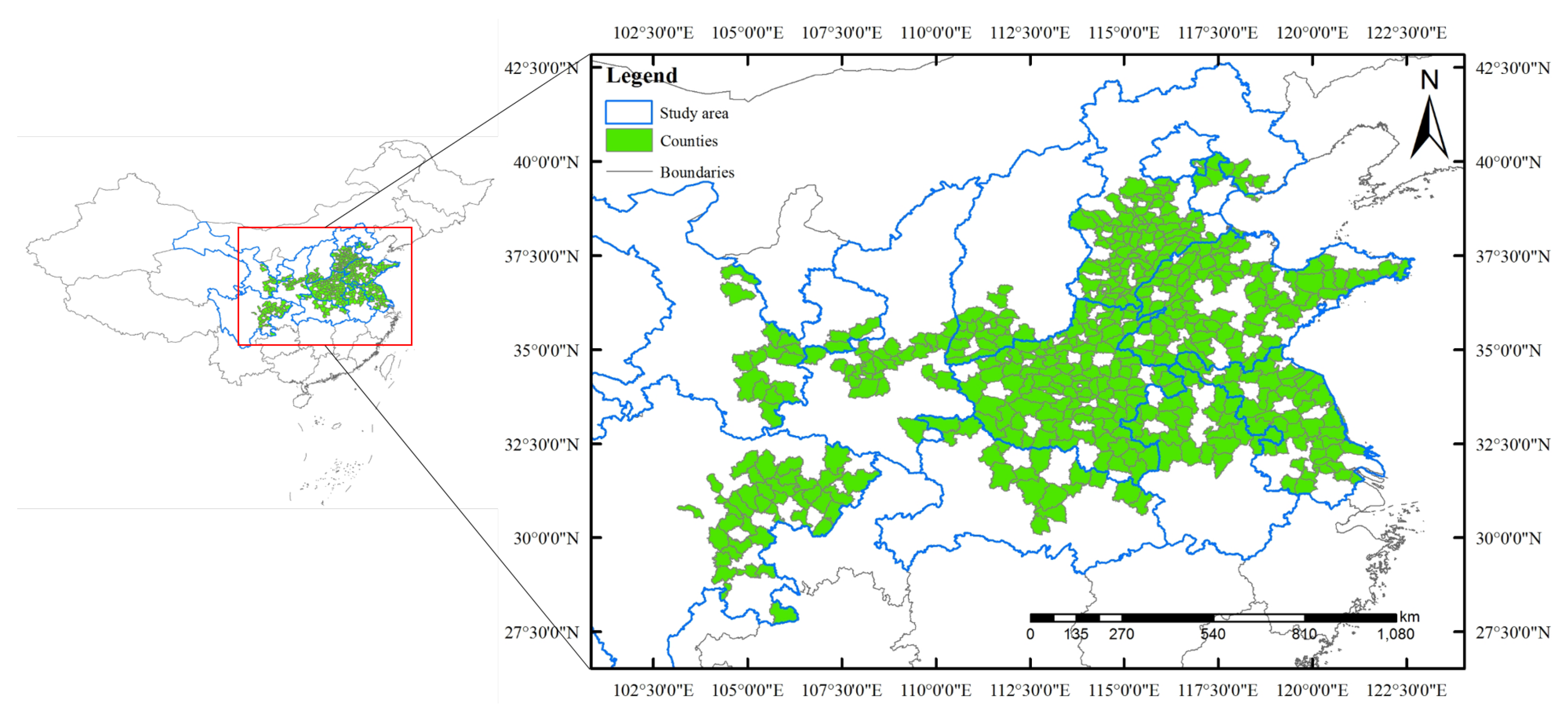
2.1. Study Area

The study focuses on winter wheat planting regions in China (Figure 1), including most areas of Hebei, Henan, Shandong, and Jiangsu province, north of Anhui and Hubei province, southwestern Shanxi province, central Shaanxi province, east of Gansu and Sichuan province, extending from 103 E to 122 E and from 28 N to 40 N. It includes two main winter wheat growing regions: the northern and the southern areas. The northern area is located to the south of the Great Wall, north of Qinling Mountain and Huaihe River, where winter wheat planting acreage and production account for 60% of the country. The northern area has a temperate continental monsoon climate, with an annual average temperature of 9–15 C and an annual rainfall of 440–980 mm. The main prevailing rotation mode is winter wheat and summer corn. The southern area is located to the south of Qinling Mountain and Huaihe River, with a subtropical monsoon climate, an annual average temperature of 16–24 C and an annual precipitation more than 1000 mm. Winter wheat is mostly rotated with paddy rice in this area.

2.2. Datasets and Preprocessing

2.2.1. Satellite Data

The Advanced Very High Resolution Radiometer (AVHRR, 0.05 arc degrees, daily) surface reflectance [38] were chosen as our satellite data source given its long-term observation and suitable temporal resolution. The bands “SREFL_CH1” (red band), “SREFL_CH2” (near-infrared band), “SREFL_CH3” (thermal infrared band), and the Normalized Difference Vegetation (NDVI) were selected as remote sensing input data.

2.2.2. Meteorological Data

Weather conditions play a vital role during crop growing season. The China Meteorological Forcing Dataset from the Institute of Tibetan Plateau Research, Chinese Academy of Sciences [39,40,41] was used as meteorological input data. This dataset provides seven meteorological variables (Table 1) including temperature, precipitation, air pressure, air specific humidity, downward shortwave radiation, downward longwave radiation, and wind speed, at a spatial resolution of 0.1 degrees and temporal resolution of 3 h. These variables are usually used as drivers for crop models to simulate the growing processes of crops, since they affect crops in different ways during growing stages. We expected to establish these effects on crops using our neural networks model.

2.2.3. Soil Data

Soil properties largely determine the spatial variability of crop yields when the weather is ideal and the crop management is in the same condition. Previous work [30] also demonstrated that soil quality is relevant for crop yield prediction, which provides complementary information and increases yield prediction accuracy. In this study, the SoilGrids dataset was used, which is a global gridded soil information dataset, with a spatial resolution of 1 km or 250 m [42,43]. We chose SoilGrids 250 m as soil inputs, which were predicted by an ensemble of machine learning methods fitted using 150,000 soil profiles and 158 remote sensing-based covariates [42]. This dataset includes nine soil features (listed in Table 1) describing the physical and chemical properties of the soil in seven layers of depth from 0 to 200 cm.

2.2.4. Cropland Data

It is difficult to obtain the specific crop planting map for all individual years from 1982 to 2015. Several previous studies [44,45,46] compared the use of a crop specific mask and generalized cropland mask for crop yield prediction. Although there could be some loss of accuracy in some cases, generalized cropland mask can still be used for crop yield prediction. Furthermore, according to the data of National Bureau of Statistics (http://data.stats.gov.cn/), winter wheat is the dominant crop in winter season over our study area, which could account for more than 90% of the total planting area among summer grain crops (Winter wheat in China is harvested in summer). Thus, cropland data were used as the wheat mask in the present study. The cropland product was downloaded from European Space Agency Climate Change Initiative (ESA CCI), which provides annual land cover maps from the year 1992 to 2015 with a spatial resolution of 300 m. This dataset is kept updating and can be used in practical application for yield prediction of current year.

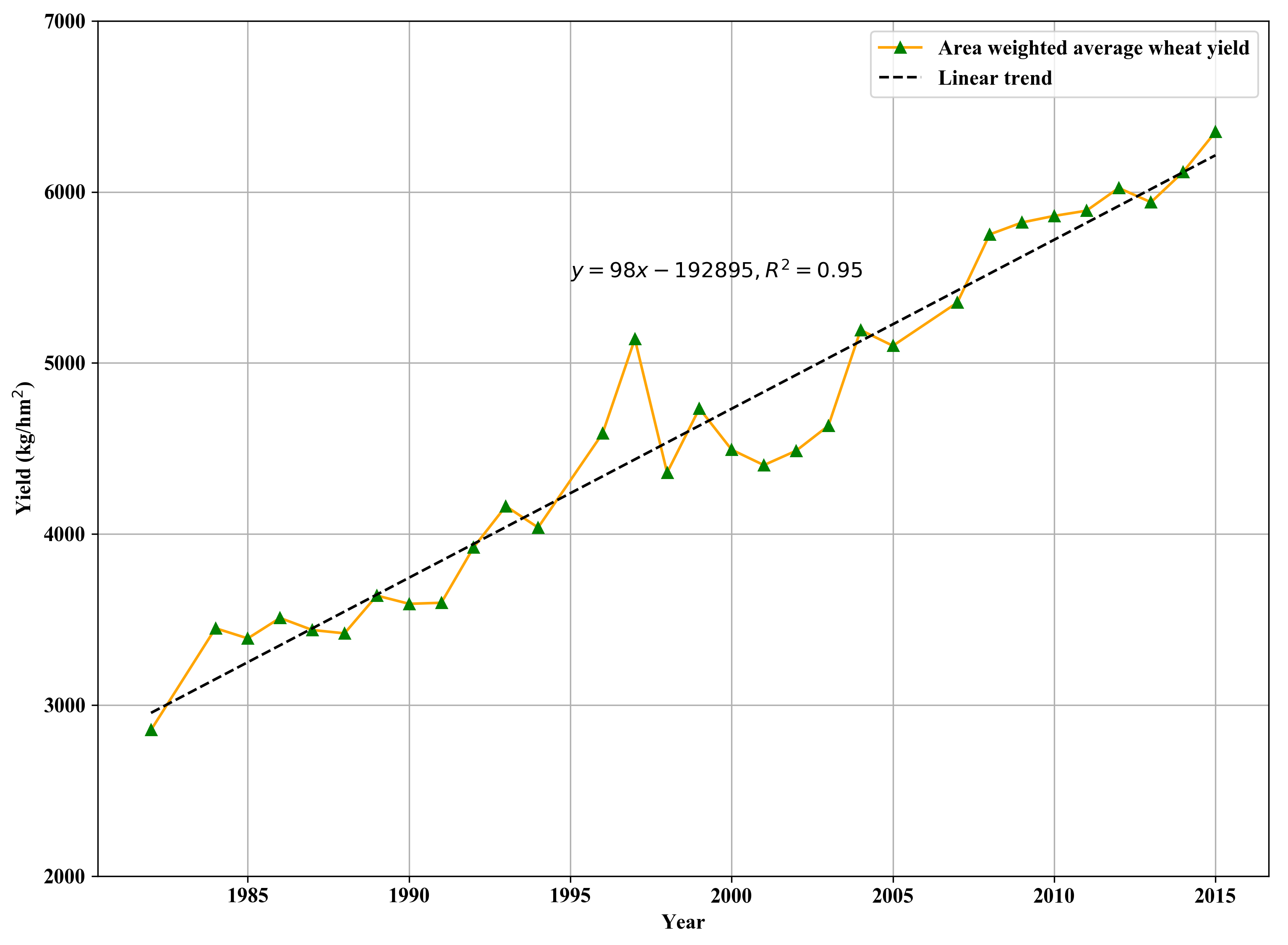
2.2.5. Yield Data and Detrending

The county-level yield data in 1982–2015 was collected manually from local statistical yearbooks which were not published online (data for the years 1983, 1995, and 2006 were missing). Counties with a winter wheat planting area greater than 10,000 ha and more than 25 years of records were selected as our modeling and analysis samples (Figure 1). There were in total 11,444 yield records after filtering.
As shown in Figure S2, the model was not able to learn the temporal trend of the yield when using the statistical yield data to train it. Thus, in hindsight, it is necessary to detrend yield data in the modeling process when the yield data are from a wide range of years. The trend of yields was assumed as linear (Figure 2) and removed while keeping the spatial variability in each year by calculating relative yields. We first calculated the area weighted average yield (kg/ha) of all counties in every year. Then, for each year, the trend yield was obtained using linear regression with weighted average yields of other years. Finally, the relative yield (Equation (1)) was applied to all county-level yield data using the trend yield in the corresponding year. Here, the trend yields can be seen as average yield level of the whole study area. The relative yield indicates the relative difference between the statistical yield at the county level and the average yield in the study area. The relative yields were used to train our deep learning model to avoid the impact of trend. In practical application, to predict the yield for an individual year, we just need to predict the relative yield using the trained model and get the trend yield of this year using linear regression as the trend was assumed to be linear. Then the predicted yield (kg/ha) can be calculated reversely using Equation (1). The distribution difference (Figure 3) between the actual yields and relative yields indicates that the yield level varies with time without detrending (Figure 3a). However, a zero-mean distribution (Figure 3b) was achieved using relative yields which means the trend is removed acceptably.
y i = y i y ¯ t r e n d y ¯ t r e n d
where y i is a single county-level yield record, and y ¯ t r e n d is the trend yield of the whole study area in the corresponding year.

2.2.6. Data Preprocessing

Remote sensing data were processed on the Google Earth Engine (GEE) [47], which is a planetary-scale platform for earth science data and analysis (The GEE code was shared https://drive.google.com/file/d/1m7-LhpfIoFU8LrvaSQGgQn00cSxV-aCt/view?usp=sharing). Meteorological data and soil data were downloaded and processed on desktop computer using GDAL (The Geospatial Data Abstraction Library). Although the surface reflectance data are daily, the time series has some missing values and fluctuates as a result of noise. To reduce the noise, we produced stable 8-day interval time series by maximum-value composite [48], and cropland masking was applied synchronously. Meteorological data were also aggregated every 8-day interval to keep the same time length as the remote sensing data. All remote sensing data, meteorological data, and soil data were spatially aggregated to the mean for each county with county boundaries. Invalid data were deleted and interpolated and each variable was normalized to 0–1 using its maximum and minimum values. Finally, all the time series had a length of 32 for each year, covering the entire growing season of winter wheat (from October to the middle of June in the following year).

2.3. Model Development

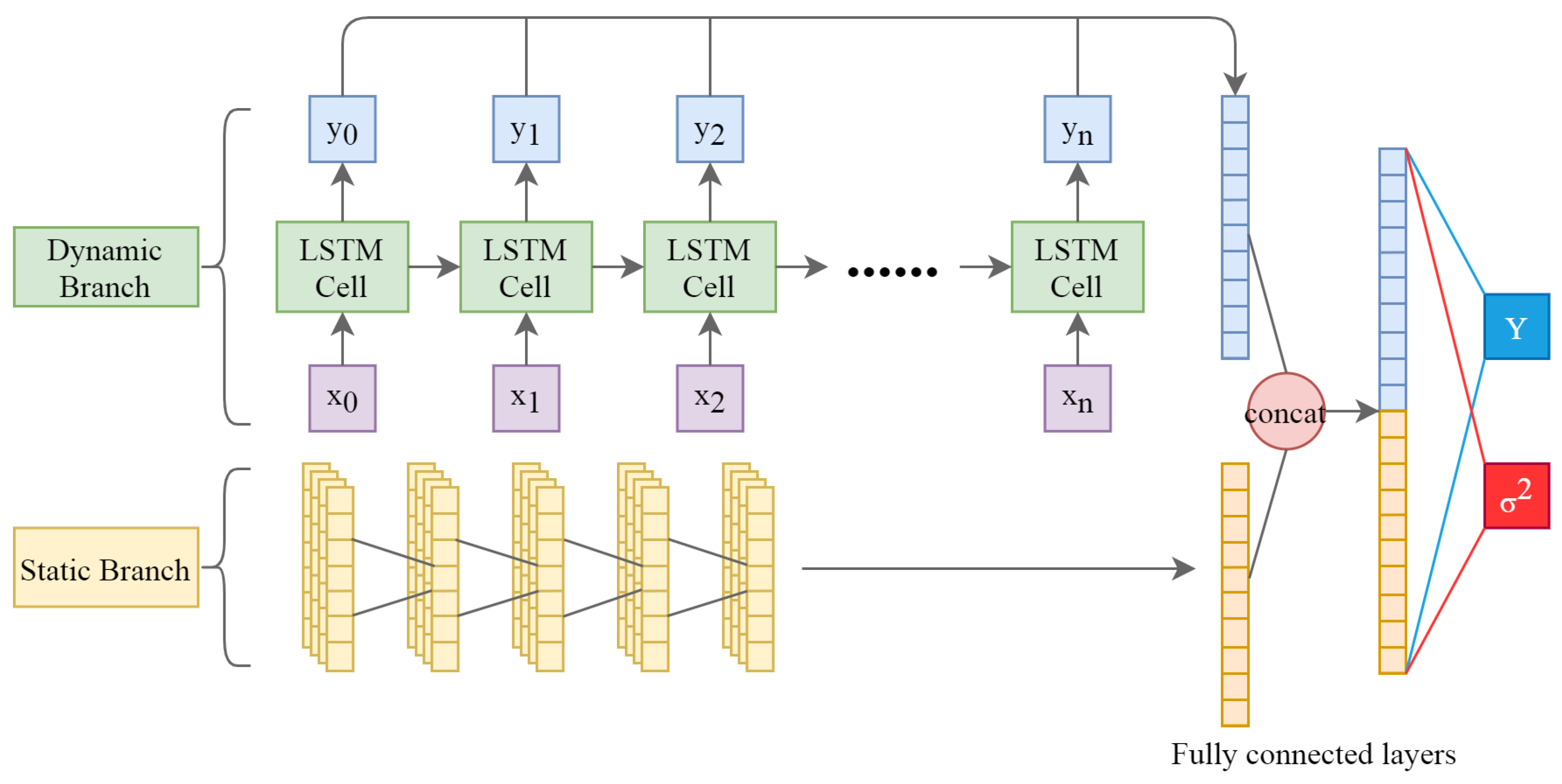
2.3.1. Deep Neural Network Structure

Remote sensing and meteorological data change dynamically during crop growing season; however, soil properties can be assumed to be constant. According to different structures of dynamic and static features, the model was split into two components (see model structure in Figure 4). The dynamic features were input into a LSTM network which is adept at processing time series data, and the static features were fed into a one-dimensional CNN to extract the vertical features from the multi-depth soil properties. The number of units in the LSTM cell was 32. As for the CNN component, there were four convolutional layers and the kernel size was 3. The dimensions of filters in these four layers were 128, 128, 256, and 256, and the strides were 1, 2, 1, 2, respectively. Both of the components were merged from the fully connected layer. The activation function is ReLU [49].

2.3.2. Quantification of Prediction Uncertainty

It is important to quantify the prediction uncertainty of the yield regression model. The prediction uncertainty can be divided into aleatoric and epistemic uncertainties on the basis of different sources [50]. Aleatoric uncertainty comes from observation noise while epistemic uncertainty accounts for the uncertainty of the model. Kendall and Gal’s [37] methods were used to estimate these two types of uncertainties in the present study.
An adjusted loss function (Equation (2)) was used to estimate heteroscedastic aleatoric uncertainty with an assumption that observation noise can vary with different samples. This was achieved by splitting the last fully connected layer into two outputs (Figure 4), therefore, both of the f ( x i ) and σ ( x i ) could be learned simultaneously. Epistemic uncertainty was estimated using Monte Carlo dropout [51], which can be interpreted as a Bayesian approximation. In practice, the model needed to dropout before every weight layer and also used the dropout at the test time for the many forward passes, which was a sampling process from the approximate posterior.
L N N ( θ ) = 1 N i = 1 N 1 2 σ ( x i ) 2 y i f ( x i ) 2 + 1 2 log σ ( x i ) 2

2.3.3. Implementation Details

We used TensorFlow (GPU version 1.15) [52], Python’s deep learning library, to construct and train our neural network model. All weights of the network were initialized by He initialization [53], and biases were initialized using zero. The loss function (Equation (2)) was used to optimize parameters. The initial learning rate was set to 0.0005 and the Adam optimizer [54] was applied to minimize the loss because of its ability to adjust the learning rate during the training stage. The batch size is 64 and the network was trained for 50 epochs, then the best model was saved during training.

2.4. Model Evaluation Metrics

We chose Normalized Root Mean Square Error (NRMSE), Coefficient Of Determination (R 2 ), and Mean Absolute Percentage Error (MAPE), the three metrics in Equations (4)–(6), and a schedule of leave-one-year-out-validation [55,56,57] to evaluate our model’s accuracy. In other words, for each year, the model was trained using yield data from other years and validated using yield data from that year. There were a total of 11,444 yield samples. The sample size for each year was not exactly the same, varying between 300 and 400. This form of validation guarantees that the prediction of the model in each year is unbiased by information of the year to be predicted. It should be noted that NRMSE is more reasonable than RMSE when the model is validated yearly because the levels of yield change with the year.
R M S E = 1 n i = 1 n y i ^ y i 2
N R M S E = R M S E y ¯
R 2 = 1 i = 1 n y i ^ y i 2 i = 1 n y i y ¯ 2
M A P E = 100 % n i = 1 n y i ^ y i y i

3. Results

3.1. Model Accuracy

Figure S2 shows the scatter plots of every year with the three accuracy metrics. Generally, the accuracy in recent years is higher than in early years. The overall R 2 , RMSE, and MAPE of all samples are 0.77, 721 kg/ha, and 15.38%, respectively, which were calculated using the predicted value of all the samples using leave-one-year-out-validation.
We also calculated the three accuracy metrics for each county in all the years. The spatial distributions of R 2 , NRMSE, and MAPE (Figure 5, Figure 6 and Figure 7) show that the R 2 values in more than 80% of counties are positive and greater than 0.5, indicating that the model can explain more than 50% of the time variability for these counties. The NRMSE and MAPE are less than 0.2 and 20% for most counties, respectively. Generally, higher errors are observed in northwestern provinces (Shanxi, Shaanxi, and Gansu) since most of the cropland in these regions is rainfed (Figure S3) and the planting density of wheat is low, while most of the North China Plain is irrigated with a high planting density. Yields in rainfed areas are generally lower than those in irrigated areas (Figure S4). Yield data from irrigated areas is much more than that from rainfed areas and the inputs of our model did not include irrigation data of different areas. Besides, the generalized cropland mask was used in this study rather than the winter wheat mask. These factors would limit the model’s performance in rainfed areas and non-wheat dominant areas. This is one of the reasons that low yields were overestimated, as shown in the scatter plots of Figure S2. Another reason could be that the sample sizes of the low yield and high yield were smaller than that of the middle yield. The model was trained by this unbalanced sample distribution, which caused the model to tend towards predicting the middle yield. In addition, training deep learning models needs a large amount of data, and the total of 11,444 samples in this study may not be sufficient to obtain better results in the low and high ends of the yield. As a result, low yields were overestimated and high yields were underestimated, especially in the early years.

3.2. Impact of Different Data Sources on Model Accuracy

To evaluate the yield prediction performance on different data sources, we performed an analysis on several combinations of data sources, and the overall accuracies are listed in Table 2. Compared with meteorological data, using remote sensing data alone achieved a higher accuracy with an R2 of 0.58, RMSE of 969 kg/ha, and MAPE of 21.04%, because remote sensing data are more direct and a more comprehensive observation of crop growing status. In addition, there is supposed to be higher accuracy if using winter wheat masks. On the other hand, most regions of the study area are irrigated, which may weaken the impact of weather conditions. The combination of remote sensing and meteorological data shows a slight increase in accuracy compared with remote sensing data alone, which means that the contributions from them are overlap to a great extent.
The accuracy shows a great improvement when soil information is added (Table 2). The overall R 2 , RMSE, MAPE values are 0.60, 945 kg/hm 2 , 19.94%, respectively, when the model was trained without the soil branch. However, these values are 0.77, 721 kg/ha, and 15.38% with the soil branch. Figure 8 shows the difference in NRMSE with and without the soil branch. There is about a 20% improvement in model accuracy, which indicates the addition of soil data improved model’s ability of capturing spatial variability of yield.
It should be noted that the soil information was constant for each county in all the years when training the model. To show whether the model is overfitted on soil information, we implemented cross-validation based on location by randomly selecting yield samples from 70% of the counties to train the model and used samples from the other counties to validate. This validation was performed ten times and average accuracy metrics were calculated using accuracy metrics of these ten times (Table 3). The results show that there is no obvious overfitting, which means the model is generalized and can be used to estimate the yield in the counties where the statistical yield is not available.

3.3. Improvement in Yield Detrending

As shown in Figure 9a, the model without the detrending yield produced highly biased results whereby the predicted yields are overestimated in the early years and underestimated in recent years, indicating the model is not able to capture the increasing trend of the yield caused by advancement in crop variety, technology, and field management. Figure 9 compares the predicted average yield of all counties in all years before and after yield detrending. When the model was trained using the relative yields, the overall R 2 , RMSE, MAPE are 0.77, 721 kg/ha, and 15.38%, while they are 0.23, 1312 kg/ha, and 24.4% without detrending (results of every year are shown in Figures S1 and S2). The improvement in accuracy is significant, and there is a more consistent trend (Figure 9b) with the statistical average yield.

3.4. Comparison with Machine Learning Methods

To further evaluate the model performance, we compared the proposed deep learning model with other machine learning methods, including random forest, support vector machine, and lasso regression, the parameters of which were optimized to reach as high an accuracy as possible. These machine learning models were performed using scikit-learn, which is a machine learning package in Python. Table 4 shows the overall accuracy of these models. The results indicate that the proposed model outperforms these machine learning approaches, because deep learning models have a better ability to model high-level feature representation through a hierarchical learning framework [58].

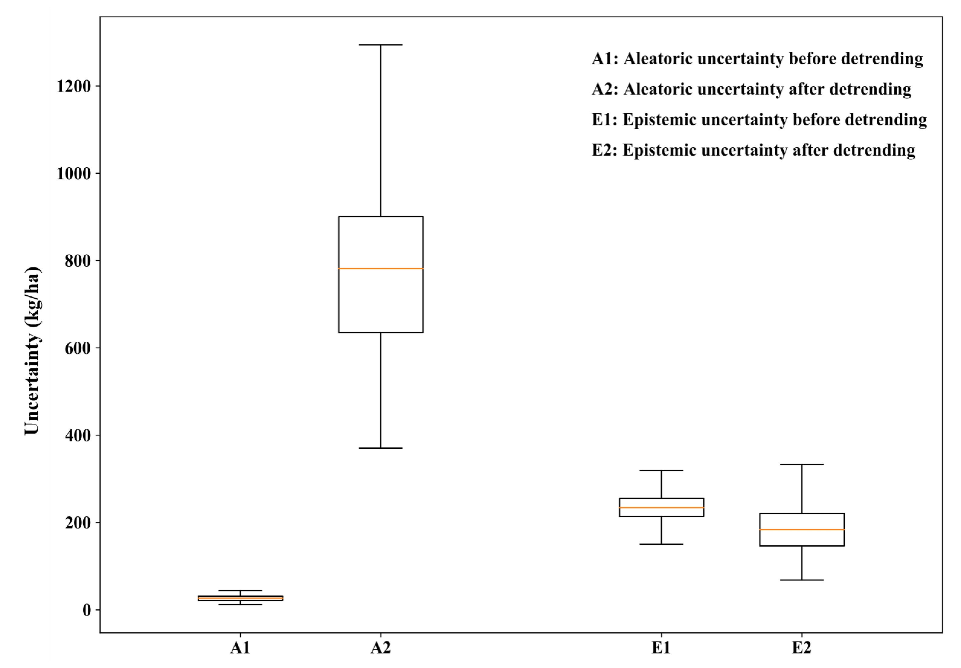
3.5. Quantified Uncertainty

As described in Section 2.3.2, the model can estimate the uncertainty of each output, which is regarded as the confidence interval of model prediction. We randomly chose some counties to show the changes of their yields and uncertainty over years in Figure 10. The scatter plots on right side of the figure indicate the prediction accuracy of these counties. It can be seen that the aleatoric uncertainty is generally greater than the epistemic uncertainty.

3.6. Yield Forecast Ability

A permutation test [59] was performed to evaluate the relative importance of different months throughout the growth period of winter wheat. By permuting the data of a specific period, if the loss of accuracy is large compared to the model with complete data, we can conclude that the data during this period has great influence on the final yield prediction. The results (Figure 11) show that April is the most important growth period, in which the heading stage of winter wheat occurs. Therefore, we trained the model using data obtained before May to test the forecast ability. The overall R 2 , RMSE, and MAPE of the prediction in early May are 0.75, 732 kg/ha, and 15.8%, respectively. There is small decrease in accuracy compared to the result using data in the full growing stages. Therefore, the results suggest that it is possible to predict wheat yield one month before harvest, indicating the high forecast ability of the model.

4. Discussion

4.1. Uncertainty Changes Caused by Yield Detrending

Although the model accuracy improved when trained by the relative yield, the aleatoric uncertainty shows a significant increase (Figure 12 ). On average, the aleatoric uncertainties before and after detrending are 27 kg/ha and 752 kg/ha, the epistemic uncertainties are 238 kg/ha and 171 kg/ha respectively. The aleatoric uncertainty before yield detrending is small and almost constant, indicating the homoscedastic aleatoric uncertainty. In contrast, it is apparent that yield detrending brings more noise to the labels and this noise varies with different samples, corresponding to heteroscedastic aleatoric uncertainty. The difference between the homoscedastic and heteroscedastic aleatoric uncertainty was explained by Gal [60] with some demonstrations. The reason for this change is that overall trend was used in our detrending method instead of trends in individual counties; however, the increasing rates of yield are different for each county. As a result, the aleatoric uncertainty rises significantly. On the other hand, the epistemic uncertainty decreased slightly. The epistemic uncertainty comes from the model structure and parameters. The decrease in epistemic uncertainty is thought to be caused by the model parameters since the model structure was the same before and after detrending. For the sample subset of each year, the joint distribution of inputs and outputs is closer to the results of all samples than those without detrending. Reduction of out-of-distribution samples in individual years helps to reduce epistemic uncertainty [37]. This change of uncertainty indicates that the deep learning model becomes more robust if trained by the relative yield. Nevertheless, the requirements for detrending could be a main limitation in this study and future studies are needed to better model the yield trend.

4.2. Impact of Agricultural Policies

Yields were overestimated with high biases during 2000 to 2003, which can be observed from the scatter plots in Figure S1 and the plot in Figure 9b. The main reason for that is the changing agricultural policies during these years. Grain supply exceeded demand and storage increased at the end of the 1990s because of the increasing production. Furthermore, the Chinese government have not issued production targets since 2001, resulting in a fast decrease in the winter wheat planting area during the adjustment of the crop planting structure. In addition, there was a stagnation of yield growth in many regions caused by the planting area reduction in low-quality and high-yield varieties, but an increase in high-quality and low-yield varieties. As a result, grain production reached a low point in 2003. In year 2004, the market grain price began to increase because of high demand and low storage. The government introduced a series of agricultural subsidy policies such as minimum purchase prices and subsidies to encourage grain production. Farmers were motivated by these policies and put more inputs such as fertilizer, pesticides, and machinery into agricultural production, making the planting area, yield, and production start to increase again [61,62].
In addition, severe agro-meteorological disasters could be another possible reason for the high biases in the yield prediction from 2000 to 2003 (Figure S1 and Figure 9b). The main hazard for winter wheat in China is drought; this is based on an analysis of the records of agro-meteorological stations and statistics [63]. However, the biases are so high that it could not even be caused by the severe drought during 2000 to 2003. Therefore, we suggest that socioeconomic factors might have a major effect on production, which was also demonstrated by Yu [64] using multiple crop models.

4.3. Potential for Integrating Prior Knowledge

In this study, we tried to build a data-driven model using the same environmental factors as most crop models. However, the fact is that most data-driven models can only capture correlation but not causality [65]. Therefore, integrating prior knowledge can improve the model performance and credibility, which can be achieved by combining submodules in process models [66,67]. For regional yield estimation in this study, the model could be constrained by some rules or physical laws that are already clearly known and described mathematically in crop models.
In addition, the influence of socioeconomic factors can also be expressed by some econometric models to fit a better yield trend than just using a linear trend with the year. Figure 13 is the linear regressed wheat yield of China using wheat planting inputs per unit area, including seeds, fertilizers, pesticides, and machinery, which were collected from “Compilation of national agricultural product cost-benefit data” of China. Although the stagnation of yield growth in the 2000–2003 period is modeled well, these kinds of data are collected afterwards, and so are not available before harvest and cannot be used to make a yield prediction. Apparently, production inputs are affected by socioeconomic factors such as market prices and agricultural subsidies, which are available prior to harvest. This makes it possible to quantitatively estimate the impact of socioeconomic factors in yield prediction by combining some econometric models.

5. Conclusions

In this study, we developed a deep learning model which combined remote sensing, meteorological, and soil data, to estimate the winter wheat yield in the main planting area of China at the county level. The model was trained using the detrended statistical yield data and evaluated by leave-one-year-out-validation, and showed a satisfactory accuracy of wheat yield prediction. Results also showed that the yield forecast could be achieved at least one month prior to harvest with a small loss of accuracy. The uncertainty analysis was further conducted using an adjusted loss function and Monte Carlo dropout. We found that yield detrending could possibly cause high uncertainty of yield prediction and should be treated carefully when applied in crop yield prediction. The proposed method exhibits great potential for applications in other crop types and agricultural landscape regions all over the world.

Supplementary Materials

The following are available online at https://www.mdpi.com/2072-4292/12/11/1744/s1, Figure S1: Winter wheat yield forecasting accuracy with deep learning model from 1982 to 2015 before detrending yield, Figure S2: Winter wheat yield forecasting accuracy with deep learning model from 1982 to 2015 after detrending yield, Figure S3: Locations of counties where MAPE is greater than 25% and the background is distribution of irrigated and rainfed areas, Figure S4: Average yield of all years for each county.

Author Contributions

Conceptualization, X.W. and J.H.; methodology, X.W.; writing—original draft preparation, X.W.; writing—review and editing, J.H., D.Y. and Q.F.; supervision, J.H. and Q.F. All authors have read and agreed to the published version of the manuscript.

Funding

This research is supported by the National Key Research and Development Program of China (project No. 2018YFE0122700), National Natural Science Foundation of China (Project No. 41671418, 41971383) and China Postdoctoral Science Foundation (Project No. 2018M641529, 2019T120155).

Conflicts of Interest

The authors declare no conflict of interest.

Abbreviations

The following abbreviations are used in this manuscript:
LAILeaf Area Index
ETEvapotranspiration
LSTMLong Short-Term Memory
CNNConvolution Neural Networks
AVHRRAdvanced Very High Resolution Radiometer
NDVINormalized Difference Vegetation Index
GEEGoogle Earth Engine
GDALThe Geospatial Data Abstraction Library
RMSERoot Mean Square Error
NRMSENormalized Root Mean Square Error
R 2 Coefficient Of Determination
MAPEMean Absolute Percentage Error

References

  1. Lobell, D.B.; Cassman, K.G.; Field, C.B. Crop yield gaps: Their importance, magnitudes, and causes. Annu. Rev. Environ. Resour. 2009, 34, 179–204. [Google Scholar] [CrossRef] [Green Version]
  2. Basso, B.; Cammarano, D.; Carfagna, E. Review of crop yield forecasting methods and early warning systems. In Proceedings of the First Meeting of the Scientific Advisory Committee of the Global Strategy to Improve Agricultural and Rural Statistics, Rome, Italy, 18 July 2013; Volume 41. [Google Scholar]
  3. Schlenker, W.; Roberts, M.J. Nonlinear effects of weather on corn yields. Rev. Agric. Econ. 2006, 28, 391–398. [Google Scholar] [CrossRef]
  4. Huang, J.; Tian, L.; Liang, S.; Ma, H.; Becker-Reshef, I.; Huang, Y.; Su, W.; Zhang, X.; Zhu, D.; Wu, W. Improving winter wheat yield estimation by assimilation of the leaf area index from Landsat TM and MODIS data into the WOFOST model. Agric. For. Meteorol. 2015, 204, 106–121. [Google Scholar] [CrossRef] [Green Version]
  5. Huang, J.; Sedano, F.; Huang, Y.; Ma, H.; Li, X.; Liang, S.; Tian, L.; Zhang, X.; Fan, J.; Wu, W. Assimilating a synthetic Kalman filter leaf area index series into the WOFOST model to improve regional winter wheat yield estimation. Agric. For. Meteorol. 2016, 216, 188–202. [Google Scholar] [CrossRef]
  6. Huang, J.; Ma, H.; Sedano, F.; Lewis, P.; Liang, S.; Wu, Q.; Su, W.; Zhang, X.; Zhu, D. Evaluation of regional estimates of winter wheat yield by assimilating three remotely sensed reflectance datasets into the coupled WOFOST–PROSAIL model. Eur. J. Agron. 2019, 102, 1–13. [Google Scholar] [CrossRef]
  7. Zhuo, W.; Huang, J.; Li, L.; Zhang, X.; Ma, H.; Gao, X.; Huang, H.; Xu, B.; Xiao, X. Assimilating soil moisture retrieved from Sentinel-1 and Sentinel-2 data into WOFOST model to improve winter wheat yield estimation. Remote Sens. 2019, 11, 1618. [Google Scholar] [CrossRef] [Green Version]
  8. Moriondo, M.; Maselli, F.; Bindi, M. A simple model of regional wheat yield based on NDVI data. Eur. J. Agron. 2007, 26, 266–274. [Google Scholar] [CrossRef]
  9. Dubey, R.; Ajwani, N.; Kalubarme, M.; Sridhar, V.; Navalgund, R.; Mahey, R.; Sidhu, S.; Jhorar, O.; Cheema, S.; Na Rang, R. Pre-harvest wheat yield and production estimation for the Punjab, India. Int. J. Remote Sens. 1994, 15, 2137–2144. [Google Scholar] [CrossRef]
  10. Huang, J.; Gómez-Dans, J.L.; Huang, H.; Ma, H.; Wu, Q.; Lewis, P.E.; Liang, S.; Chen, Z.; Xue, J.H.; Wu, Y.; et al. Assimilation of remote sensing into crop growth models: Current status and perspectives. Agric. For. Meteorol. 2019, 276, 107609. [Google Scholar] [CrossRef]
  11. Wall, L.; Larocque, D.; Léger, P.M. The early explanatory power of NDVI in crop yield modelling. Int. J. Remote Sens. 2008, 29, 2211–2225. [Google Scholar] [CrossRef]
  12. Becker-Reshef, I.; Vermote, E.; Lindeman, M.; Justice, C. A generalized regression-based model for forecasting winter wheat yields in Kansas and Ukraine using MODIS data. Remote Sens. Environ. 2010, 114, 1312–1323. [Google Scholar] [CrossRef]
  13. Franch, B.; Vermote, E.; Becker-Reshef, I.; Claverie, M.; Huang, J.; Zhang, J.; Justice, C.; Sobrino, J. Improving the timeliness of winter wheat production forecast in the United States of America, Ukraine and China using MODIS data and NCAR Growing Degree Day information. Remote Sens. Environ. 2015, 161, 131–148. [Google Scholar] [CrossRef]
  14. Doraiswamy, P.C.; Moulin, S.; Cook, P.W.; Stern, A. Crop yield assessment from remote sensing. Photogramm. Eng. Remote Sens. 2003, 69, 665–674. [Google Scholar] [CrossRef]
  15. Patrício, D.I.; Rieder, R. Computer vision and artificial intelligence in precision agriculture for grain crops: A systematic review. Comput. Electron. Agric. 2018, 153, 69–81. [Google Scholar] [CrossRef] [Green Version]
  16. Feng, Q.; Liu, J.; Gong, J. UAV remote sensing for urban vegetation mapping using random forest and texture analysis. Remote Sens. 2015, 7, 1074–1094. [Google Scholar] [CrossRef] [Green Version]
  17. Feng, Q.; Liu, J.; Gong, J. Urban flood mapping based on unmanned aerial vehicle remote sensing and random forest classifier—A case of Yuyao, China. Water 2015, 7, 1437–1455. [Google Scholar] [CrossRef]
  18. Ali, I.; Greifeneder, F.; Stamenkovic, J.; Neumann, M.; Notarnicola, C. Review of machine learning approaches for biomass and soil moisture retrievals from remote sensing data. Remote Sens. 2015, 7, 16398–16421. [Google Scholar] [CrossRef] [Green Version]
  19. Ip, R.H.; Ang, L.M.; Seng, K.P.; Broster, J.; Pratley, J. Big data and machine learning for crop protection. Comput. Electron. Agric. 2018, 151, 376–383. [Google Scholar] [CrossRef]
  20. Jeong, J.H.; Resop, J.P.; Mueller, N.D.; Fleisher, D.H.; Yun, K.; Butler, E.E.; Timlin, D.J.; Shim, K.M.; Gerber, J.S.; Reddy, V.R.; et al. Random forests for global and regional crop yield predictions. PLoS ONE 2016, 11, e0156571. [Google Scholar] [CrossRef]
  21. Han, J.; Zhang, Z.; Cao, J.; Luo, Y.; Zhang, L.; Li, Z.; Zhang, J. Prediction of Winter Wheat Yield Based on Multi-Source Data and Machine Learning in China. Remote Sens. 2020, 12, 236. [Google Scholar] [CrossRef] [Green Version]
  22. Kuwata, K.; Shibasaki, R. Estimating corn yield in the united states with modis evi and machine learning methods. ISPRS Ann. Photogramm. Remote Sens. Spat. Inf. Sci. 2016, 3. [Google Scholar] [CrossRef] [Green Version]
  23. Kim, N.; Lee, Y.W. Machine learning approaches to corn yield estimation using satellite images and climate data: A case of Iowa State. J. Korean Soc. Surv. Geod. Photogramm. Cartogr. 2016, 34, 383–390. [Google Scholar] [CrossRef]
  24. Feng, Q.; Yang, J.; Zhu, D.; Liu, J.; Guo, H.; Bayartungalag, B.; Li, B. Integrating Multitemporal Sentinel-1/2 Data for Coastal Land Cover Classification Using a Multibranch Convolutional Neural Network: A Case of the Yellow River Delta. Remote Sens. 2019, 11, 1006. [Google Scholar] [CrossRef] [Green Version]
  25. Hochreiter, S.; Schmidhuber, J. Long short-term memory. Neural Comput. 1997, 9, 1735–1780. [Google Scholar] [CrossRef]
  26. You, J.; Li, X.; Low, M.; Lobell, D.; Ermon, S. Deep gaussian process for crop yield prediction based on remote sensing data. In Proceedings of the Thirty-First AAAI Conference on Artificial Intelligence, San Francisco, CA, USA, 4–9 February 2017. [Google Scholar]
  27. Wang, A.X.; Tran, C.; Desai, N.; Lobell, D.; Ermon, S. Deep transfer learning for crop yield prediction with remote sensing data. In Proceedings of the 1st ACM SIGCAS Conference on Computing and Sustainable Societies, Menlo Park and San Jose, CA, USA, 20–22 June 2018; pp. 1–5. [Google Scholar]
  28. Wolanin, A.; Mateo-García, G.; Camps-Valls, G.; Gómez-Chova, L.; Meroni, M.; Duveiller, G.; Liangzhi, Y.; Guanter, L. Estimating and understanding crop yields with explainable deep learning in the Indian Wheat Belt. Environ. Res. Lett. 2020, 15, 024019. [Google Scholar] [CrossRef]
  29. Jiang, Z.; Liu, C.; Hendricks, N.P.; Ganapathysubramanian, B.; Hayes, D.J.; Sarkar, S. Predicting county level corn yields using deep long short term memory models. arXiv 2018, arXiv:1805.12044. [Google Scholar]
  30. Oliveira, I.; Cunha, R.L.; Silva, B.; Netto, M.A. A scalable machine learning system for pre-season agriculture yield forecast. arXiv 2018, arXiv:1806.09244. [Google Scholar]
  31. Qin, X.; Zhang, F.; Liu, C.; Yu, H.; Cao, B.; Tian, S.; Liao, Y.; Siddique, K.H. Wheat yield improvements in China: Past trends and future directions. Field Crops Res. 2015, 177, 117–124. [Google Scholar] [CrossRef]
  32. Wang, F.; He, Z.; Sayre, K.; Li, S.; Si, J.; Feng, B.; Kong, L. Wheat cropping systems and technologies in China. Field Crops Res. 2009, 111, 181–188. [Google Scholar] [CrossRef]
  33. Li, X.; Liu, N.; You, L.; Ke, X.; Liu, H.; Huang, M.; Waddington, S.R. Patterns of cereal yield growth across China from 1980 to 2010 and their implications for food production and food security. PLoS ONE 2016, 11, e0159061. [Google Scholar] [CrossRef]
  34. Quiring, S.M.; Papakryiakou, T.N. An evaluation of agricultural drought indices for the Canadian prairies. Agric. For. Meteorol. 2003, 118, 49–62. [Google Scholar] [CrossRef]
  35. Michel, L.; Makowski, D. Comparison of statistical models for analyzing wheat yield time series. PLoS ONE 2013, 8, e78615. [Google Scholar] [CrossRef] [PubMed] [Green Version]
  36. Lu, J.; Carbone, G.J.; Gao, P. Detrending crop yield data for spatial visualization of drought impacts in the United States, 1895–2014. Agric. For. Meteorol. 2017, 237, 196–208. [Google Scholar] [CrossRef]
  37. Kendall, A.; Gal, Y. What uncertainties do we need in Bayesian deep learning for computer vision? In Proceedings of the NIPS 2017—2017 Conference on Neural Information Processing Systems, Long Beach, CA, USA, 4–9 December 2017; pp. 5575–5585. [Google Scholar]
  38. Vermote, E.; Justice, C.; Csiszar, I.; Eidenshink, J.; Myneni, R.; Baret, F.; Masuoka, E.; Wolfe, R.; Claverie, M. NOAA Climate Data Record (CDR) of AVHRR Surface Reflectance, Version 5; NOAA National Centers for Environmental Information: Washington, DC, USA, 2019. Available online: https://doi.org/10.7289/V53776Z4 (accessed on 1 December 2019).
  39. Chen, Y.; Yang, K.; He, J.; Qin, J.; Shi, J.; Du, J.; He, Q. Improving land surface temperature modeling for dry land of China. J. Geophys. Res. Atmos. 2011, 116. [Google Scholar] [CrossRef]
  40. Yang, K.; He, J.; Tang, W.; Qin, J.; Cheng, C.C. On downward shortwave and longwave radiations over high altitude regions: Observation and modeling in the Tibetan Plateau. Agric. For. Meteorol. 2010, 150, 38–46. [Google Scholar] [CrossRef]
  41. Kun, Y. China Meteorological Forcing Dataset (1979–2018); National Tibetan Plateau Data Center, Institute of Tibetan Plateau Research, Chinese Academy of Sciences: Beijing, China, 2018. [Google Scholar] [CrossRef]
  42. Hengl, T.; de Jesus, J.M.; Heuvelink, G.B.; Gonzalez, M.R.; Kilibarda, M.; Blagotić, A.; Shangguan, W.; Wright, M.N.; Geng, X.; Bauer-Marschallinger, B.; et al. SoilGrids250m: Global gridded soil information based on machine learning. PLoS ONE 2017, 12, e0169748. [Google Scholar] [CrossRef] [Green Version]
  43. Hengl, T.; de Jesus, J.M.; MacMillan, R.A.; Batjes, N.H.; Heuvelink, G.B.; Ribeiro, E.; Samuel-Rosa, A.; Kempen, B.; Leenaars, J.G.; Walsh, M.G.; et al. SoilGrids1km—Global soil information based on automated mapping. PLoS ONE 2014, 9, e105992. [Google Scholar] [CrossRef] [Green Version]
  44. Shao, Y.; Campbell, J.B.; Taff, G.N.; Zheng, B. An analysis of cropland mask choice and ancillary data for annual corn yield forecasting using MODIS data. Int. J. Appl. Earth Obs. Geoinf. 2015, 38, 78–87. [Google Scholar] [CrossRef]
  45. Zhang, Y.; Chipanshi, A.; Daneshfar, B.; Koiter, L.; Champagne, C.; Davidson, A.; Reichert, G.; Bédard, F. Effect of using crop specific masks on earth observation based crop yield forecasting across Canada. Remote Sens. Appl. Soc. Environ. 2019, 13, 121–137. [Google Scholar] [CrossRef]
  46. Liu, J.; Shang, J.; Qian, B.; Huffman, T.; Zhang, Y.; Dong, T.; Jing, Q.; Martin, T. Crop Yield Estimation Using Time-Series MODIS Data and the Effects of Cropland Masks in Ontario, Canada. Remote Sens. 2019, 11, 2419. [Google Scholar] [CrossRef] [Green Version]
  47. Gorelick, N.; Hancher, M.; Dixon, M.; Ilyushchenko, S.; Thau, D.; Moore, R. Google Earth Engine: Planetary-scale geospatial analysis for everyone. Remote Sens. Environ. 2017. [Google Scholar] [CrossRef]
  48. Holben, B.N. Characteristics of maximum-value composite images from temporal AVHRR data. Int. J. Remote Sens. 1986, 7, 1417–1434. [Google Scholar] [CrossRef]
  49. Nair, V.; Hinton, G.E. Rectified linear units improve restricted boltzmann machines. In Proceedings of the 27th International Conference on Machine Learning (ICML-10), Haifa, Israel, 21–24 June 2010; pp. 807–814. [Google Scholar]
  50. Kiureghian, A.D.; Ditlevsen, O. Aleatory or epistemic? Does it matter? Struct. Saf. 2009, 31, 105–112. [Google Scholar] [CrossRef]
  51. Gal, Y.; Ghahramani, Z. Dropout as a Bayesian approximation: Representing model uncertainty in deep learning. In Proceedings of the 33rd International Conference on Machine Learning, ICML 2016, New York, NY, USA, 19–24 June 2016; Volume 3, pp. 1651–1660. [Google Scholar]
  52. Abadi, M.; Agarwal, A.; Barham, P.; Brevdo, E.; Chen, Z.; Citro, C.; Corrado, G.S.; Davis, A.; Dean, J.; Devin, M.; et al. TensorFlow: Large-Scale Machine Learning on Heterogeneous Systems. 2015. Available online: tensorflow.org (accessed on 11 July 2019).
  53. He, K.; Zhang, X.; Ren, S.; Sun, J. Delving Deep into Rectifiers: Surpassing Human-Level Performance on ImageNet Classification. In Proceedings of the 2015 IEEE International Conference on Computer Vision (ICCV), Santiago, Chile, 7–13 December 2015; pp. 1026–1034. [Google Scholar] [CrossRef] [Green Version]
  54. Kingma, D.P.; Ba, J. Adam: A method for stochastic optimization. arXiv 2014, arXiv:1412.6980. [Google Scholar]
  55. Bolton, D.K.; Friedl, M.A. Forecasting crop yield using remotely sensed vegetation indices and crop phenology metrics. Agric. For. Meteorol. 2013, 173, 74–84. [Google Scholar] [CrossRef]
  56. Schut, A.; Stephens, D.; Stovold, R.; Adams, M.; Craig, R. Improved wheat yield and production forecasting with a moisture stress index, AVHRR and MODIS data. Crop Pasture Sci. 2009, 60, 60–70. [Google Scholar] [CrossRef]
  57. Mkhabela, M.; Bullock, P.; Raj, S.; Wang, S.; Yang, Y. Crop yield forecasting on the Canadian Prairies using MODIS NDVI data. Agric. For. Meteorol. 2011, 151, 385–393. [Google Scholar] [CrossRef]
  58. LeCun, Y.; Bengio, Y.; Hinton, G. Deep learning. Nature 2015, 521, 436–444. [Google Scholar] [CrossRef]
  59. Breiman, L. Statistical modeling: The two cultures (with comments and a rejoinder by the author). Stat. Sci. 2001, 16, 199–231. [Google Scholar] [CrossRef]
  60. Gal, Y. Uncertainty in Deep Learning. Ph.D. Thesis, University of Cambridge, Cambridge, UK, 2016. [Google Scholar]
  61. Zhu, X. Analysis of China’s Grain Supply and Demand Balance. Probl. Agric. Econ. 2004, 4, 12–19. [Google Scholar] [CrossRef]
  62. Li, Y.; Zhang, W.; Ma, L.; Wu, L.; Shen, J.; Davies, W.J.; Oenema, O.; Zhang, F.; Dou, Z. An analysis of China’s grain production: Looking back and looking forward. Food Energy Secur. 2014, 3, 19–32. [Google Scholar] [CrossRef]
  63. Zhang, Z.; Wang, P.; Zhang, S.; Tao, F.; Liu, X. Spatio-temporal changes of agrometrorological disasters for wheat production across China since 1990. Acta Geogr. Sin. 2013, 68. [Google Scholar] [CrossRef]
  64. Yu, C.; Huang, X.; Chen, H.; Huang, G.; Ni, S.; Wright, J.S.; Hall, J.; Ciais, P.; Zhang, J.; Xiao, Y.; et al. Assessing the Impacts of Extreme Agricultural Droughts in China Under Climate and Socioeconomic Changes. Earth’s Future 2018, 6, 689–703. [Google Scholar] [CrossRef]
  65. Schölkopf, B. Causality for Machine Learning. arXiv 2019, arXiv:cs.LG/1911.10500. [Google Scholar]
  66. Reichstein, M.; Camps-Valls, G.; Stevens, B.; Jung, M.; Denzler, J.; Carvalhais, N. Deep learning and process understanding for data-driven Earth system science. Nature 2019, 566, 195–204. [Google Scholar] [CrossRef]
  67. Jia, X.; Willard, J.; Karpatne, A.; Read, J.; Zwart, J.; Steinbach, M.; Kumar, V. Physics guided RNNs for modeling dynamical systems: A case study in simulating lake temperature profiles. In Proceedings of the 2019 SIAM International Conference on Data Mining, Calgary, AB, Canada, 2–4 May 2019; pp. 558–566. [Google Scholar]
Figure 1. The study area which is the main winter wheat producing areas in China.
Remotesensing 12 01744 g001
Figure 2. The yearly area weighted average yield calculated from county-level yields in the whole study area and its linear trend.
Remotesensing 12 01744 g002
Figure 3. A comparison between the distributions of actual wheat yields and relative yields from 1982 to 2015 in central China.
Remotesensing 12 01744 g003
Figure 4. Overall structure of the deep learning model for wheat yield forecasting.
Remotesensing 12 01744 g004
Figure 5. Spatial distribution of the Coefficient Of Determination (R 2 ) calculated from the predicted yields of all the years for each county. The inset panel in the upper left is the histogram of R 2 .
Remotesensing 12 01744 g005
Figure 6. Spatial distribution of the Normalized Root Mean Square Error (NRMSE) calculated from the predicted yields of all the years for each county. The inset panel in the upper left is the histogram of NRMSE.
Remotesensing 12 01744 g006
Figure 7. Spatial distribution of the Mean Absolute Percentage Error (MAPE) calculated from the predicted yields of all the years for each county. The inset panel in the upper left is the histogram of MAPE.
Remotesensing 12 01744 g007
Figure 8. Effect of soil information on accuracy. “Change of NRMSE” is the improvement in NRMSE with the addition of soil data.
Remotesensing 12 01744 g008
Figure 9. The predicted average yield of all counties before and after detrending. The red solid line is the average yield of all county-level yield data. (a) The predicted average yield of all counties before detrending; (b) The predicted average yield of all counties after detrending.
Remotesensing 12 01744 g009
Figure 10. Predicted results of three randomly chosen counties.
Remotesensing 12 01744 g010
Figure 11. Loss of model accuracy after permuting data of different months compared to the model using complete data.
Remotesensing 12 01744 g011
Figure 12. Uncertainty changes before and after detrending yield.
Remotesensing 12 01744 g012
Figure 13. Linear regressed yield of China with input in agricultural production per Ha. The red line is the wheat yield of China collected from Nation Bureau of Statistics. The blue line is the linear regressed yield using agricultural inputs. The green oval contains the results of 2000–2003.
Remotesensing 12 01744 g013
Table 1. Detailed information of the input features.
Data SourceFeature NameUnitDescription
Remote sensing data of AVHRRSREFL_CH1 Surface reflectance (640 nm)
SREFL_CH2 Surface reflectance (860 nm)
SREFL_CH3 Surface reflectance (3750 nm)
NDVI Normalized Difference Vegetation Index
Meteorological dataTEMPKInstantaneous near surface (2 m) air temperature
PRECmm hr 1 Precipitation rate
PRESPaInstantaneous near surface (2 m) air pressure
SHUMkg kg 1 Instantaneous near surface (2 m) air specific humidity
LRADW m 2 Surface downward longwave radiation
SRADW m 2 Surface downward shortwave radiation
WINDm s 1 Instantaneous near surface (10 m) wind speed
Soil dataBLDFIEkg m 3 Bulk density (fine earth)
CECSOLcmolc kg 1 Cation exchange capacity of soil
CLYPPT%Clay content (0–2 micrometer) mass fraction
CRFVOL%Coarse fragments volumetric
ORCDRCg kg 1 Soil organic carbon content (fine earth fraction)
PHIHOX PH × 10 in H2O
PHIKCL PH × 10 in KCL
SLTPPT%Silt content (2-50 micrometer) mass fraction
SNDPPT%Sand content (50-2000 micrometer) mass fraction
Table 2. Model accuracy using different combinations of data sources.
Combination of Data SourcesR 2 RMSE (kg/hm 2 )MAPE
Remote sensing data0.5896921.04%
Meteorological data0.50105122.20%
Remote sensing data, Meteorological data0.6094519.94%
Remote sensing data, Meteorological data and soil data0.7772115.28%
Table 3. Cross-validation of model with a random split from ten rounds. For each round, samples of 70% of the counties were used to train, the other samples were used to validate.
RoundDatasetR 2 RMSE (kg/ha)MAPE (%)
train0.8264313.03
1test0.7570614.81
change−0.07+63+1.78
train0.8263013.03
2test0.7775816.04
change−0.05+128+3.01
train0.8558812.15
4test0.7472715.15
change−0.11+139+3.00
train0.8360812.84
5test0.8166813.85
change−0.02+60+1.01
train0.8460712.87
6test0.7375315.08
change−0.11+146+2.21
train0.8460912.17
7test0.7966514.45
change−0.05+56+2.28
train0.8363113.08
8test0.7668113.85
change−0.07+50+0.77
train0.8459512.83
9test0.7474013.83
change−0.1+145+1.00
train0.8361813.17
10test0.7672415.34
change−0.07+106+2.17
train0.8361412.77
Averagetest0.7671214.63
change−0.07+98+1.86
Table 4. Model accuracy using different combinations of data sources.
MethodR 2 RMSE (kg/hm 2 )MAPE
Proposed0.7772115.28%
Random Forest0.7279217.03%
Support Vector Machine0.5798120.30%
Lasso Regression0.6094920.52%

