Detecting Ephemeral Objects in SAR Time-Series Using Frozen Background-Based Change Detection

Abstract

Change detection (CD) in SAR (Synthethic Aperture Radar) images has been widely studied in recent years and has become increasingly attractive due to the growth of available datasets. The potential of CD has been shown in different fields, including disaster monitoring and military applications. Access to multi-temporal SAR images of the same scene is now possible, and therefore we can improve the performance and the interpretation of CD. Apart from specific SAR campaign measurements, the ground truth of the scene is usually unknown or only partially known when dealing with open data. This is a critical issue when the purpose is to detect targets, such as vehicles or ships. Indeed, typical change detection methods can only provide relative changes; the actual number of targets on each day cannot be determined. Ideally, this change detection should occur between a target-free image and one with the objects of interest. To do so, we propose to benefit from pixels’ intrinsic temporal behavior to compute a frozen background reference (FBR) image and perform change detection from this reference image. We will then consider that the scene consists only of immobile objects (e.g., buildings and trees) and removable objects that can appear and disappear from acquisition to another (e.g., cars and ships). Our FBR images will, therefore, aim to estimate the immobile background of the scene to obtain, after change detection, the exact amount of targets present on each day. This study was conducted first with simulated SAR data for different number of acquisition dates and Signal-to-Noise Ratio (SNR). We presented an application in the region of Singapore to estimate the number of ships in the study area for each acquisition.

1. Introduction

SAR (Synthetic Aperture Radar) images change detection is a promising solution for target detection when dealing with high cluttered environments, such as urban areas, forests, or harbors. Indeed, typical CFAR (Constant False Alarm Rate) detectors computed on single images also provide the scatterers that belong to the background and can fail to detect targets due to the high clutter level relative to the target response [1].

SAR images change detection (CD) has been widely studied, for instance, in bi-date cases and for multi-temporal data in [2,3]. Typical bi-date based change detection approaches represent a relative change between the combination of acquisitions. As such, it might lead to misinterpretation, for example, if the target was present during the two acquisitions or when a target overlaps on two different dates. Such processing implies that, for every new image acquired, the algorithm needs to be recomputed on the whole time-series.

In the case of multi-temporal change detection, previous works detected the most significant change that occurred during the time series with knowledge of the change point as in [4]. However, in dense activity areas, such as industrial harbor or parking, several objects can overlap in the time domain and cannot be highlighted with such methods. We propose here to introduce a new change detection framework based on the computation of a frozen background reference (FBR) image, taking into account the multi-temporal capabilities of the new sensors. To do so, we consider that a scene consists of two classes of objects: ephemeral objects (targets that can move from one acquisition to another, such as cars) and immovable objects (e.g., trees and buildings).

First, several aspects of multi-temporal SAR will be discussed. Afterward, the computation of this FBR image will be detailed, and the statistical properties of such images will be studied. The objective is to identify the stable part of each pixel within the temporal domain and generate the FBR image. We propose to achieve this through the use of a time variation coefficient. Thus, a list of stable candidate pixels was built and used for change detection. This approach was tested first on simulated complex Gaussian images and then on real SAR image configurations, and results are presented for the detection of ephemeral objects in the context of maritime surveillance.

2. Multitemporal Change Detection

Remote Sensing is increasingly attractive to the scientific community as well as to governmental institutions in different domains. Several SAR times series are currently available, and even more will be in open access in the future [5,6]. Therefore, it is essential to develop methodologies and concepts to deal with this critical amount of data and extract the information in our interest. The CD between two dates has been thoroughly studied [7]; the associated statistics related have been derived in the past. For a few years, the amount of open data acquired periodically has been increasing and provides a large amount of data that has to be processed automatically depending on the application and needs of users. MCD (multitemporal change detection) has been as well studied. Statistical tests have been derived in two different forms: a multi-bidate detection that can provide information on the number of changes within the time series, or another form that provides binary information over the whole time series.

2.1. Multi-Bidate Detection Approach

This framework of change detection introduced by [3] performs a bi-date CD sequentially or combinatorially (all possible dates combinations). Then the output results represent different classes according to the sum of changes or the possible combination of changes occurring within the time-series. We present the representation of such a framework in Figure 1.

This method, however, does not consider the temporal statistics of the pixels since they are computed for a bi-date combination. It is not possible to retrieve the current ephemeral objects at a specific date because it is a relative procedure. Finally, for each new acquisition, the whole dataset has to be recomputed, increasing the computational cost.

2.2. Variation Coefficient Based CD

The variation coefficient (CV), also known as the relative standard deviation, is mathematically defined in probability theory and statistics by $\sigma /\mu$, where $\sigma$ is the standard deviation of the signal and $\mu$ the mean value. It can be considered as a normalized measurement of the dispersion of a probability distribution. A thorough study can be found in [4].

In radar images, it is commonly accepted that the amplitude of a speckle without texture follows the Rayleigh–Nakagami law:

$$RN[\mu ,L]\left(u\right)=\frac{2\sqrt{L}}{\mu \mathsf{\Gamma }\left(L\right)}{\left(\frac{\sqrt{L}u}{\mu }\right)}^{2L-1}{e}^{-{\left(\frac{\sqrt{L}}{\mu }u\right)}^2}$$

(1)

where $\mu$ is a form parameter, $\mathsf{\Gamma }$ is the gamma function, and L is called the looks number. In our approach, we are interested in time statistics.

According to [4], we can write the theoretical variation coefficient as follows:

$$CV=\sqrt{\frac{\mathsf{\Gamma }\left(L\right)\mathsf{\Gamma }(L+1)}{\mathsf{\Gamma }{(L+\frac{1}{2})}^2}-1}.$$

(2)

This expression shows that the coefficient of variation has the same value for all stable speckle zones, whatever the average amplitude of this speckle. Also, the variance of the CV decreases with a variation in $\sqrt{D}$, with D being the number of dates of the time-series.

2.3. Electromagnetical and Statistical Stability

The concept of electromagnetic stability can be expressed by a high coherence of a deterministic scatterer within the time series, usually known as permanent scatterer (PS) in interferometry. The related temporal variation coefficient is then low, and the coherence between two acquisitions is supposedly high. However, the coherence in low-intensity areas (roads, plane surfaces, and shadows) is also low, giving no further information about the temporal stability of such areas. In the case of a stable speckle, the related variation coefficient is also low, but it does not necessarily have a coherent temporal behavior in the electromagnetic point of view. It is said to be statistically stable because the parameter of its probability density function does not vary with time. The temporal variation coefficient then gives us the opportunity to obtain both electromagnetically and statistically stable pixels within the time series.

In the case of vehicle detection, it can be a keen interest for the user to know at a specific date how many targets were present in a scene, for example, for harbor monitoring or ground surveillance applications. The purpose of remote sensing is to provide images of ground scenes without the need for a physical presence; however, as the main drawback, we cannot know precisely the state of a scene at a specific date. As the ground truth is usually unknown, a CD strategy with two dates becomes difficult to establish because the content of both images remains unknown. The main idea of this method is to extract a stable temporal pattern of a scene to build its ground truth blindly: the scene is composed of all immobile objects that are electromagnetically or statistically stable in time. Afterward, each image of the scene is compared with this reference scene through change detection algorithms.

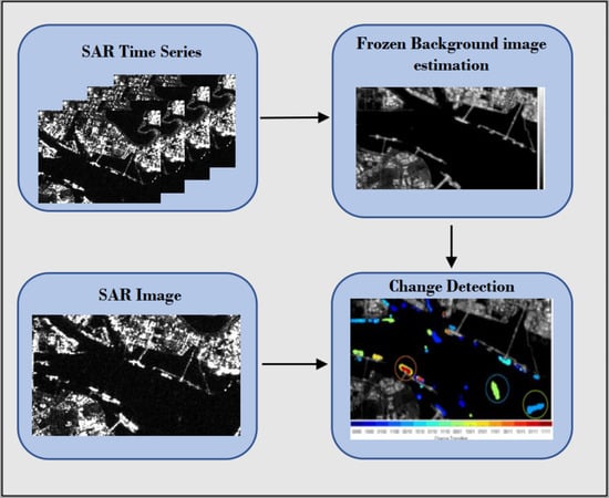
3. Frozen Background Reference Image from a Temporal Stack of Radar Images

The study aims to compute the FBR image consisting only of the signature of immovable objects and speckle noise. We want to obtain all the temporal pixels that are electromagnetically or statistically stable within the time series. This reference image is used afterward for change detection on a stack of SAR images. The resulting complex image is said to be a reference image because it aims to represent a target-free scene with only background pixels stable in time. The concept for such a reference image is presented in Figure 2. The proposed framework of change detection relies on a simple hypothesis. Within a SAR time-series, it is more likely that a given pixel stays temporally unoccupied by an ephemeral object; if not, it is considered as a background object.

3.1. Computation of the FBR Image

We define S as the matrix for a full polarization SAR image. We note i and j as the range and azimuth indices. For D acquisition dates, we note the temporal matrix $X=\left[S\right(1)\dots S(D\left)\right]$. The variation coefficient CV($X_{i,j}$) is then computed iteratively over each pixel of this temporal matrix in order to extract its stable behavior. At each iteration m, we obtain a new output matrix ${\tilde{X}}_{i,j}^m$ with $D^{\prime }<D$ dates consisting only of pixels representing stable temporal behavior. Figure 3 presents the diagram used to perform such a process.

At the end of the process, we obtain a cube with an inhomogeneous dimension in the time direction with only selected stable candidate pixels for each range and azimuth. We illustrate such results in the Figure 4. Since the stable candidate pixels of the time series have been chosen, we can assume that any random pixel of the list can be taken as a stable background pixel. This image can be computed differently depending on the situation. For instance, it is possible to create an FBR image with only random pixels of the remaining candidate pixels or by taking the mean of these remaining pixels.

3.2. CV Threshold Computation

As presented in Section 2.2, the theoretical variation coefficient depends only on L (the number equivalent of look) that can be estimated as proposed in [8]. It can be as well used directly according to the SAR acquisition for sentinel 1 GRD product L = 4.9. As discussed, the variance of the CV is a function of $\frac{1}{\sqrt{(}D)}$ with D being the number of dates in the time series. The threshold is then defined using the theoretical variation coefficient in Equation (2):

$${\mathsf{\Psi }}^m(i,j)=CV+\frac{\alpha }{\sqrt{D^m(i,j)}}$$

(3)

where $\alpha$ is a parameter to control the probability of false alarm (PFA) and $D^m(i,j)$ is the remaining number of stable dates for each range i and azimuth j at the iteration m. The threshold can be set independent of the number of the remaining images by choosing $\alpha =0$.

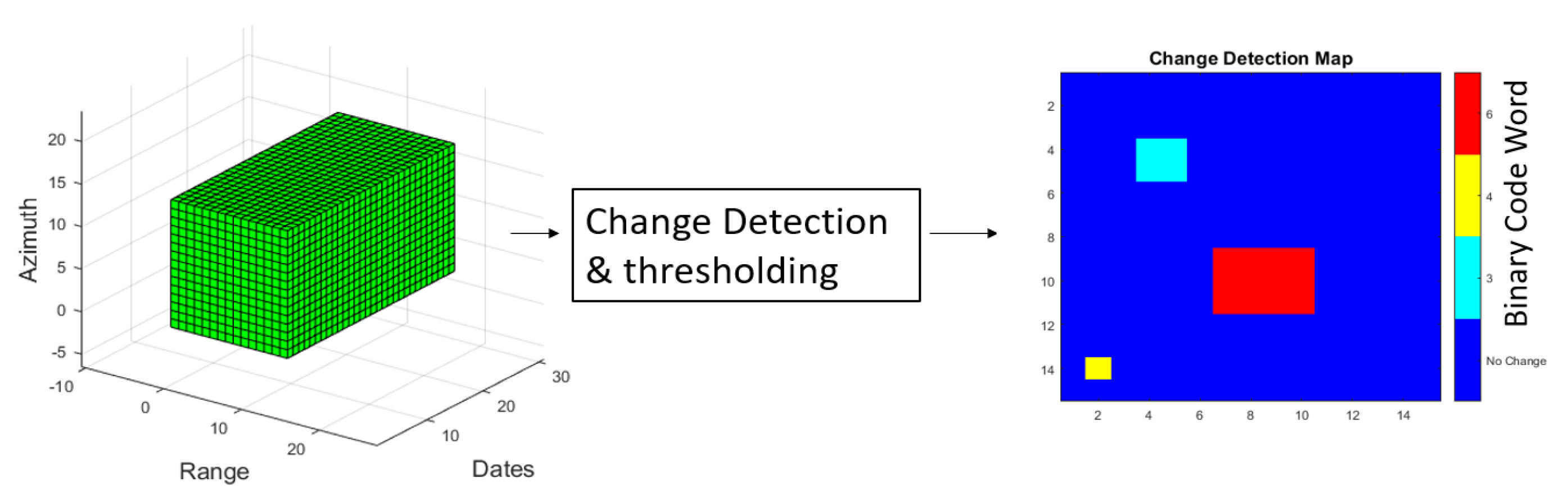
3.3. Strategies of Change Detection for Different Computation Modes of the FBR Image

Depending on the computation, it is possible to obtain the FBR image, whether from the coherent mean of each remaining candidate pixels or a single temporal random pixel for each azimuth and range.

3.3.1. Random Pixels

We chose first to select a random pixel from the list of temporal stable candidate pixels for each azimuth and range of the image. We obtained, therefore, our FBR image ${\tilde{X}}^{\left(RP\right)}$. Assuming that the statistics of speckle remained unchanged, in the space domain (range, azimuth) as well as in the time domain, we can adapt the different tests introduced in [2]. For classical change detection, we assume that the pixels of the FBR Image ${\tilde{X}}^{\left(RP\right)}$ and the Mission Image Y follow a multivariate zero-mean complex Gaussian distribution with ${\mathit{C}}_{\mathit{ref}}$ and ${\mathit{C}}_{\mathit{Y}}$ as the covariance matrices associated to vectors ${\tilde{X}}^{\left(RP\right)}$ and Y [2]. The test to be computed and compared with a threshold and can be written using the following equation:

$${\gamma }_{RP}=\frac{|{\mathit{C}}_{\mathit{ref}}{|}^N{\left|{\mathit{C}}_{\mathit{Y}}\right|}^N}{|\frac{1}{2}({\mathit{C}}_{\mathit{ref}}+{\mathit{C}}_{\mathit{Y}}){|}^{2N}}$$

(4)

where N is the number of samples within the averaging box to compute the covariance matrix, and $\left|\right|$ represents the determinant of the matrix.

3.3.2. Modified Process with Multi-Temporal Pixels

An alternative is to use the remaining pixels of the FBR image to build a modified process FBR image, ${\tilde{X}}^{\left(MP\right)}$. We consider that the modified sample covariance matrix ${\mathit{C}}_{\mathit{ref}}^{\mathit{MP}}$ has been computed on a different number of samples $N_c(i,j)$ that corresponds to the remaining number of pixel candidates for each azimuth and range:

$${\gamma }_{MP}(i,j)=\frac{|{\mathit{C}}_{\mathit{ref}}^{\mathit{MP}}{|}^{N_c(i,j)}{\left|{\mathit{C}}_{\mathit{Y}}\right|}^N}{{\left|\frac{N_c(i,j)}{N_c(i,j)+N}{\mathit{C}}_{\mathit{ref}}^{\mathit{MP}}+\frac{N}{N_c(i,j)+N}{\mathit{C}}_{\mathit{Y}})\right|}^{(N_c(i,j)+N)}}.$$

(5)

3.4. Advantages and Drawbacks of the Method

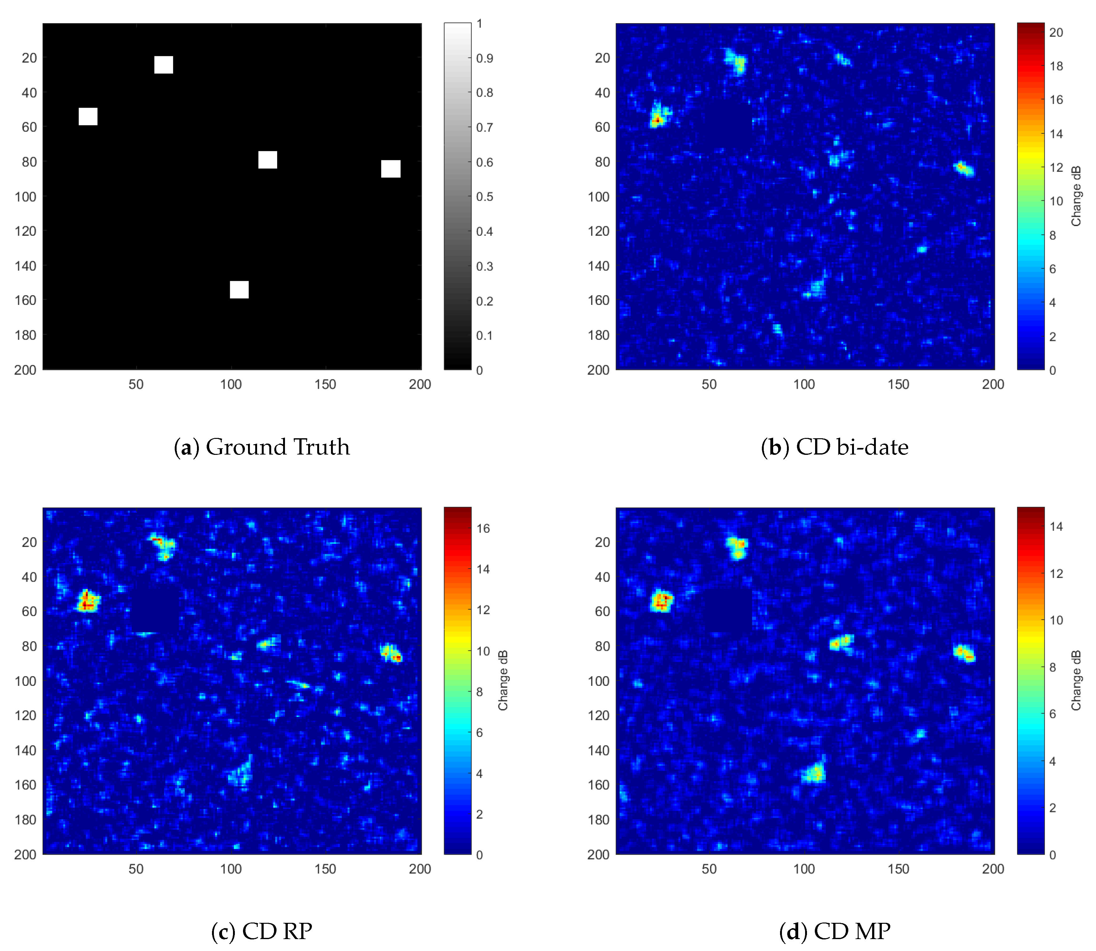
In the context of target detection in SAR images, this method can give a visualization of ephemeral objects detected at a given date. The CD output is not a relative change between two unknown dates but represents a change between an estimated temporal stationary background and an image with possible ephemeral objects. Once the FBR image is computed, it can be directly compared with new incoming images and included in automatic processing without computing the algorithm on the whole time-series. This study focuses on ephemeral target detection. In the case of a permanent change occurring in the time series, such as building construction or building destruction, the outcome would give a permanent change. This permanent change is unwanted and would end as a misinterpretation. However, it can be overcome by strategies of FBR update with a trigger on a consecutive established detection of changes.

4. Simulation

A simulated time series of SAR images is computed with a static object on the whole time series corresponding to a building (big red square in Figure 5). The settings for this simulation are presented in

Table 1. Simulation settings: with SNR (Signal-to-Noise ratio), RP (Random pixel), MP (Multi-temporal pxiels).

Simulation Parameters	Section 4.1	Section 4.2
Image Number	10	1, 3, 6, 9, 15, 20
Images size	200 × 200 pixels	200 × 200 pixels
Building size	20 × 20 pixels	20 × 20 pixels
Targets size	10 × 10 pixels	10 × 10 pixels
SNR building	13 dB	13 dB
SNR targets	3, 6, 13 dB	3 dB
Algorithms	Bi-date, RP, MP	Bi-date, RP, MP

. At a given date, five targets appear, as shown in Figure 5b with a target Signal-to-Noise ratio SNR = 6 dB. Several random target-free scenes with only the static object were generated. An example is shown in Figure 5a. The distribution of the noise is supposed to follow a zero-mean complex Gaussian distribution. From this time series of 10 simulated images, FBR scenes are computed both in RP (Random pixel) and MP (Multi-temporal pixels) modes, and Figure 5c,d present the two FBR images.

To estimate the impact of the process on the probability density functions of FBR images, we computed the histograms of both FBR images and a target-free image.

As we can see in Figure 6, histograms of RP FBR images and one random target-free scene of the stack have comparable behavior. On the contrary, as expected, the histogram of the MP FBR image is squeezed because the variance decreases with a factor $\sqrt{D}$, with D being the number of remaining stable dates.

FBR images were computed, and we will now present the behavior of the change detection results between images with target and the FBR images compared with classical bi-date change detection. The Table 1 presents the different settings used to evaluate the CD results in paragraph Section 4.1 and Section 4.2.

4.1. Impact of Target SNR

First, a set of 10 images was created. We aimed to evaluate the behavior of the detection approaches for different target SNRs. The raw output of change detection for the worst case of target SNR is presented in Figure 7, and the associated ROC (Receiver operating characteristic) curves for different configurations of the target SNR are plotted in Figure 8. The PD (detection probability) and PFA (probability of false alarm) are defined as follows: $PD=\frac{TP}{NT}$ and $PFA=\frac{FP}{NB}$ with TP as the number of pixels truly detected as a target, $NT$ as the number of ground truth pixels detected as a target, $FP$ as the number of pixels falsely detected as a target, and $NB$ as the number of pixels defined as background pixels.

As we can see in Figure 8, the CD from the RP computation of the FBR image gave a similar detection capability to the classical bi-date detection. Using the MP computation for the reference gave more improvement on change detection, especially when target SNR was low, as we can see in Figure 8e,f.

At a fixed PFA = ${10}^{-3}$, we can observe the associated probability of detection in different cases. When the SNR is sufficiently high (13 dB), results are in the same range of PD for the three different detectors: 0.75 for Bidate CD and ${\gamma }_{RP}$ and slightly higher for ${\gamma }_{MP}$ with 0.85. In the case of a lower SNR of 6 dB, the detection performances of CD-bidate and ${\gamma }_{RP}$ decreased drastically to 0.3, on the contrary, ${\gamma }_{MP}$ still gave a good PD of 0.7. Finally, in the case of a low SNR = 3 dB, The PD of the CD-bidate and ${\gamma }_{RP}$ decreased to 0.15. The probability of detection of ${\gamma }_{MP}$ was still higher but remained a poor detection probability of 0.4. The result is particularly of interest for targets hidden in high clutter, for example, in FoPen applications or urban areas. In the following part, we simulated targets with a constant SNR. The CD output will be investigated for different numbers of images within the time series using the MP method.

4.2. Impact of the Number of Available Dates

To evaluate the benefit of using several dates for the computation of the FBR scenes, several change maps were produced using the simulated ground truth with different amounts of images randomly chosen from the simulated SAR stack. The results are shown in Figure 9a,b. We can observe that the detection was improved when increasing the number of dates taken as a reference.

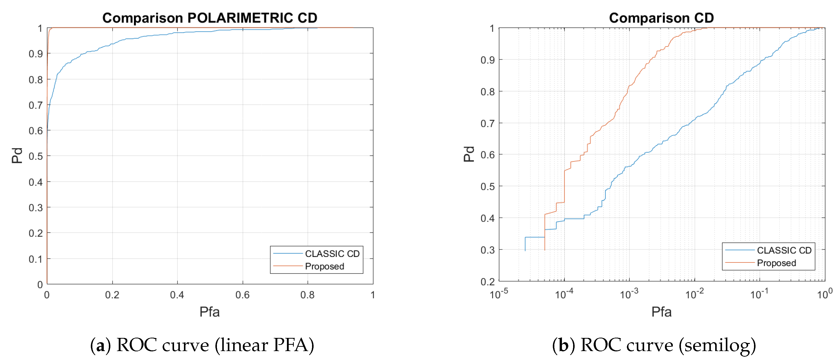
4.3. Polarimetric Case

In this part, we present the results with the framework used in the case of polarimetric data so that channels HH, HV, and VV (H stands for Horizontal and V for Vertical) will be gathered in one polarimetric vector. The process proposed in 3.1 was performed on each channel independently, and a new reference polarimetric vector was composed. We present the result in Figure 10.

From this simulation study, we can conclude on different aspects of the method. First, the choice of a random pixel RP within the candidate pixels from simulation gave comparable results to a typical bi-date detection. However, the interpretation of CD results was improved as only the ephemeral objects are seen in the resulting image. Considering the use of all remaining candidate pixels through the MP method, we can see that the detection capability was drastically better when the target SNR was decreasing. This property was a promising result for the detection of targets hidden in a high cluttered environment.

5. Results on Real SAR Data

As an illustration, a scene with boats (floating platform) on water was chosen to test our approach. A second, more complex example was selected in an industrial harbor area near Singapore.

5.1. Floating Platform over a Lake in the Area of San Francisco

This example focuses on floating platforms over sea surfaces that can have different configurations, as shown in Figure 11. The characteristics of the images used for the study are presented in

Table 2. UAVSAR (Uninhabited Aerial Vehicle Synthetic Aperture Radar) data acquisitions characteristics used for the study.

Technical Characteristics of the Sentinel Images
Acquisition Mode	PolSAR
Processing level	Single Look Complex (SLC)
Polarisation	(HH+HV+VH+VV)
Resolution	1.8 × 0.8 m
Wavelength	L-Band
Stack Name	SDelta_23518_01
Acquisition dates	June 2009 to June 2010
Location	https://www.google.com/maps/search/?api=1&query=38.052500001,-121.83250000

.

The scene under study is composed of 12 L-band fully polarimetric UAVSAR (Uninhabited Aerial Vehicle Synthetic Aperture Radar) images in the region around San Francisco. Figure 12a is the first radiometric HH image of the temporal stack, and Figure 12b,c are the FBR images obtained from our method using the RP and MP methods. The images are represented in gray levels from −30 to 0 dB.

As we can observe in this reference image, the targets were successfully removed. Figure 13a presents the results of the usual change detection between two dates of the stack. Red values on the image indicate that a significant change of amplitude occurred, whereas blue areas reflect areas with no changes.

Floating platforms were present at both dates, but not precisely in the same position; thus, the resulting image was difficult to interpret. In Figure 13b–e we plotted the results of change detection from the FBR images in RP and MP modes and the two dates that were used previously for the classical bi-date change detection. In both results, we can directly see a better quality for the image, and it is possible to more accurately identify the targets present at each date. In that case, the SNR of the boat was high; therefore, the results in RP and MP modes were similar as they are presented in the simulation of a high SNR target. This example shows that it is possible to use this method in the case of target detection, especially when it is necessary to know the number of targets present on one image without knowledge of the scene. As we can also notice, the signal to noise ratio was improved, and the targets were more easily identifiable.

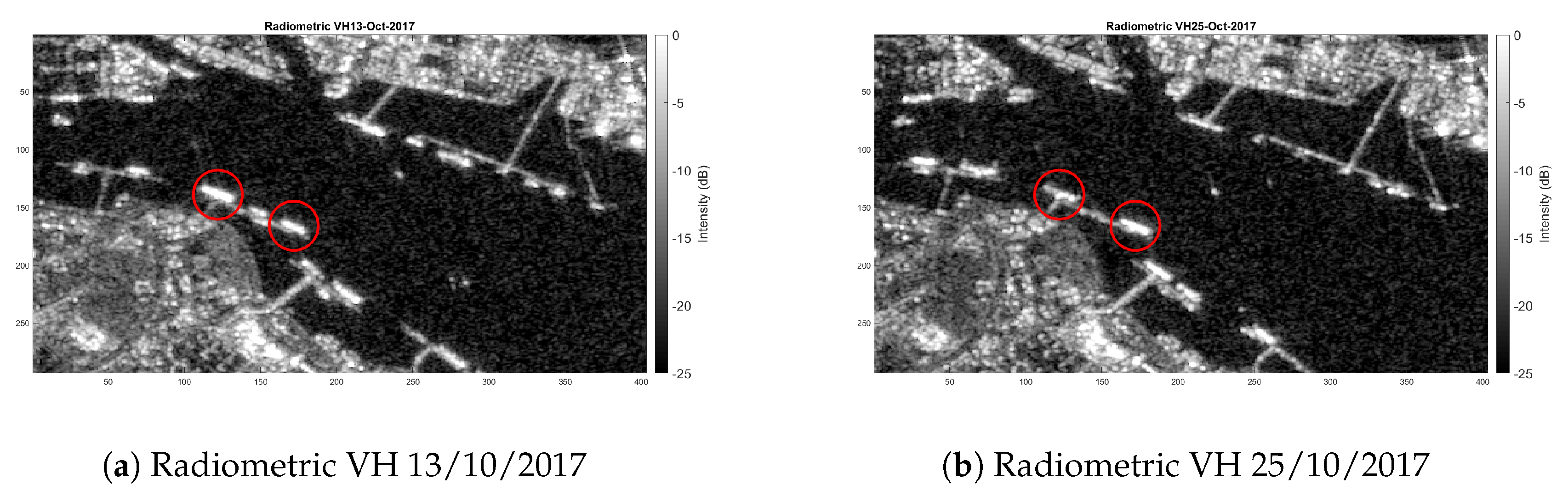
5.2. Singapore Region Study

A more complex area was chosen in Singapore in the industrial harbor of Jurong Island. Figure 14 shows the FBR image computed using 83 Sentinel GRD (Ground Range Detected) Images of Singapore projected on Google Earth in order to validate the reference scene. The characteristics of the Sentinel data used in this study can be found in

Table 3. Sentinel 1 data acquisition characteristics used for the study.

Technical Characteristics of the Sentinel Images
Acquisition mode	Interferometric Wide (IW) swath
Processing level	Level-1 Ground Range Detected
Polarisation	VV+VH
Resolution	10 × 10 m
Swath width	250 km
wavelength	C-Band
Relative orbit Number	171
Near Incidence Angle	30°
Far Incidence Angle	46°
Acquisition dates	From 3 Feb.2017 to 26 Dec. 2019
Location	http://maps.google.com/maps?q=1.294152,103.733984

. In addition, the Figure A2 represents the operations performed for each GRD image of the stack. The stack was afterward coregistrated according to the first image of the stack using the function <<Coregistration>> of SNAP (Sentinel Application Platform) software [9]. Since the environment is constituted of man-made structures, we chose to use SAR images with always the same configuration of observation, and thus the same orbit number. Indeed, most man-made structures cannnot be considered to possess an azimuthal symmetry and a subtle change in the observation angle can drastically affect their back-scattered signals. Using different orbits to compute the FBR image might corrupt the estimation of the stable background.

The study of harbors is a challenge in terms of target detection; indeed, metallic structures are associated with high scattering contributions. For instance, it is challenging to discriminate mooring quays and actual boats. Besides, the number of ships evolves from a date to another. Some ships can remain in the same position during several acquisitions, but also different ships can occupy the same pixels on consecutive acquisitions. This partial or full overlapping in time can produce misinterpretation in the CD results with classical methods. This example is a direct application of the FBR procedure to estimate a stable background within the observed scene and detect only ephemeral objects at each acquisition. Such information can be useful, for instance, if it is possible to link the number of ships parked in harbors and ports with the economic state of a region.

The FBR scene is presented using gray levels. Figure 15 also presents the zoom of the FBR scene in the area of interest. From left to right are shown the Google Maps image, then the Radiometric image with Google Maps in 50% transparency and finally, on the right, the FBR image. The FBR image matched well with the Google Earth ground truth, the metallic moorings gave strong radiometric signals and were visible on the reference image. The full-size FBR image computed using the HV channel can be found in Figure A1 in the Appendix A.

To study the number of images needed in this particular case to consider a stable background, we proposed the generation of 79 FBR images by successively incrementing the number of images on which the FBR image was calculated from 4 to 83. We then proposed to calculate ${\gamma }_{FBR}$ for the CD between each successive generated FBR image and defined the mean error as $\overline{ϵ}=\frac{1}{N_{range}{N}_{az}}{\sum }_{i=1}^{N_{range}}{\sum }_{j=1}^{N_{az}}{\gamma }_{FBR}(i,j)$ with $\overline{ϵ}$ as the mean error, $N_{range}$ and $N_{az}$ as the number of pixels in range and azimuth, respectively. As we can see from Figure 16, after 30 dates used to generate the FBR image, any new image added to compute the FBR image only slightly impacted the resulting FBR image.

5.2.1. Bi-Date Change Detection Analysis

We focused on the configuration of temporally superimposed targets, this time adjacent to a permanent scatterer (mooring quays).

In Figure 17, we can observe ships, circled in red, that share the same position during the two acquisitions and adjacent to mooring quays. We can notice from these images that most of the ships present in the scene are moored to the quays. In this configuration, the detection of boats is rendered difficult, contrary to the open sea case. The change detection was computed as previously in Section 5.1 with the two consecutive dates of Figure 17 for classical bi-date change detection and then separately with the computed FBR image.

From the classical bi-date change detection shown in Figure 18a,b, the boats were indeed not appearing in the detection map as there was time overlapping. Within the FBR CD maps, Figure 18c–f, it is possible to identify them more easily since the CD was operated from the FBR image which was a target free scene. The interpretation was, therefore, improved, and the CD map gave more consistent results when the user was interested in evaluating the ephemeral target content at a specific date.

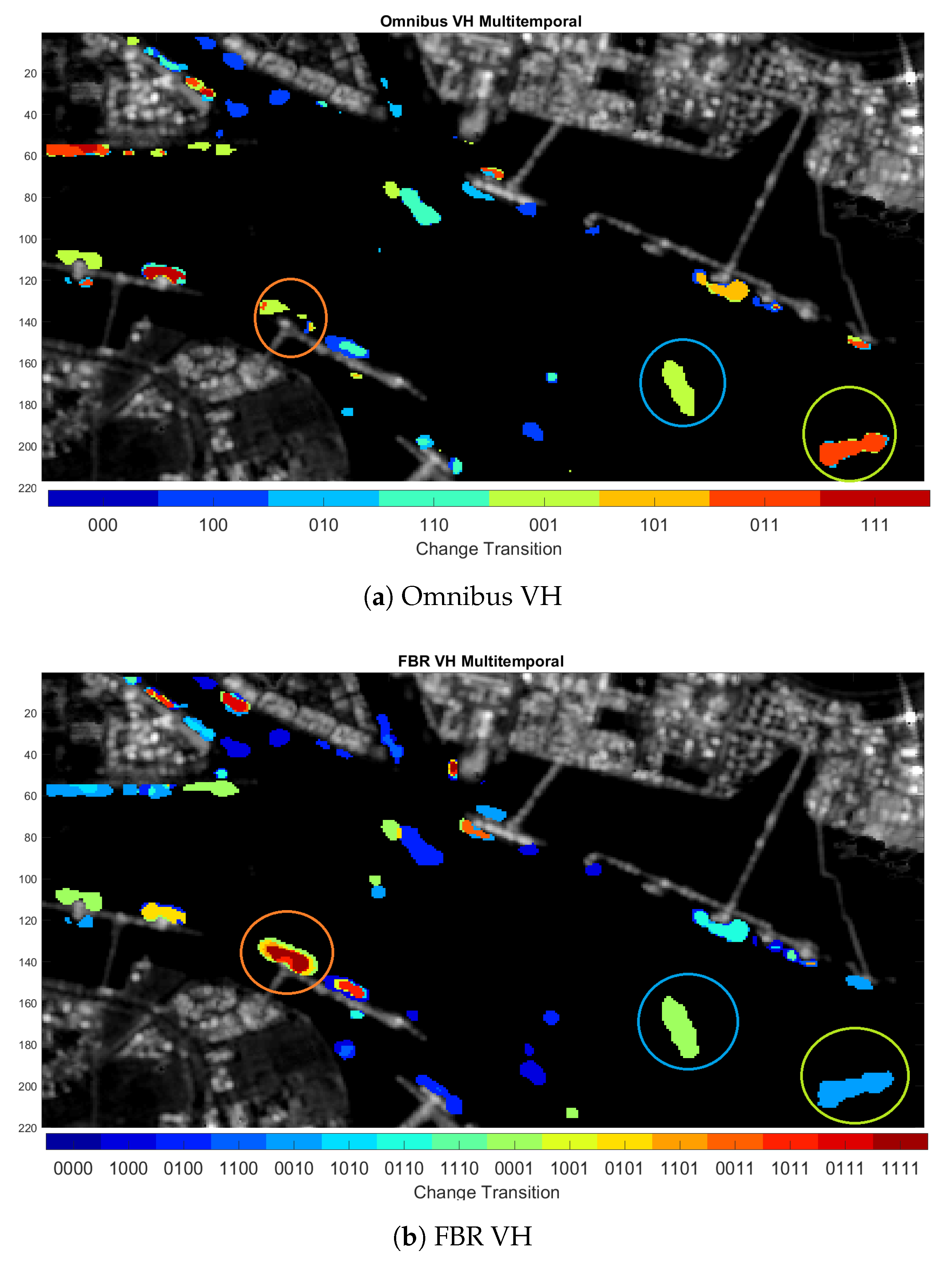
5.2.2. Multitemporal Change Detection Analysis

The classical Omnibus method sequentially performed a bi-date change detection so that we could obtain code-words relative to a specific sequence of changes. In the same way, we could obtain code-words comparing each image of the time series with the FBR image. For the sake of simplicity and ease of the interpretations, we presented the result for the HV channel on the first four images of the stack. These four images can be found in Figure A4. The results are presented in Figure 19a for the typical Omnibus procedure and in Figure 19b for the FBR change detection framework we proposed. For the result shown in Figure 19a, the obtained code-word corresponds to the transition between sequential bi-dates. Since four dates were chosen, three tests were performed sequentially to create the code-word $A_{1\to 2}^{\left(1\right)}{A}_{2\to 3}^{\left(2\right)}{A}_{3\to 4}^{\left(3\right)}$ where $A_{n\to n+1}^{\left(n\right)}$ corresponds to the binary outcome of the test between date n and n+1.

For the result shown in Figure 19b, the obtained code-word corresponded to the outcome of the test between our FBR image and the current scene. Since four dates were chosen, four tests were performed sequentially to create the code-word $B_{FBR\to 1}^{\left(1\right)}{B}_{FBR\to 2}^{\left(2\right)}{B}_{FBR\to 3}^{\left(3\right)}{B}_{FBR\to 4}^{\left(4\right)}$ where $B_{FBR\to n}^{\left(n\right)}$ corresponds to the binary outcome of the test between the FBR image and the date n. This outcome can be then interpreted as 0 if no target is present and 1 if a target is present.

We focused on the three different scenarios circled within Figure 19. The area circled in light green gave a code word “011” for the Omnibus test in Figure 19a since a boat appeared at date 3 and disappeared at date 4. The results of the FBR procedure in Figure 19b gave “0010” since the target was only present on date 3.

The area circled in blue gave a code-word “001” for the Omnibus test in Figure 19a since the boat appeared on date 4 and was not present on date 3. The results of the FBR procedure in Figure 19b gave “0001” since the target was only present on date 4.

The area circled in orange was a high attendance zone where ships were present for each acquisition from date 1 to date 4. The result with the Omnibus test was difficult to interpret due to the partial and total target overlapping between each acquisition. With the FBR procedure, the outcome is “1111” near the mooring quay since targets have been detected at each date. However, the size of targets may vary from acquisition to another, so different code-words are found around the center of detection. In general, the interpretation of such a map is not convenient due to the high number of possible combinations (maximum $2^{(D-1)}$ with D dates), and this remains a problem. The type of representation typically depends on the application.

The main advantage of the proposed method is that it is possible to retrieve the information relative to ephemeral targets at a specific date. For instance, if the amount of changes has been judged unusual, a direct CD image is available for the specific date improving the interpretation.

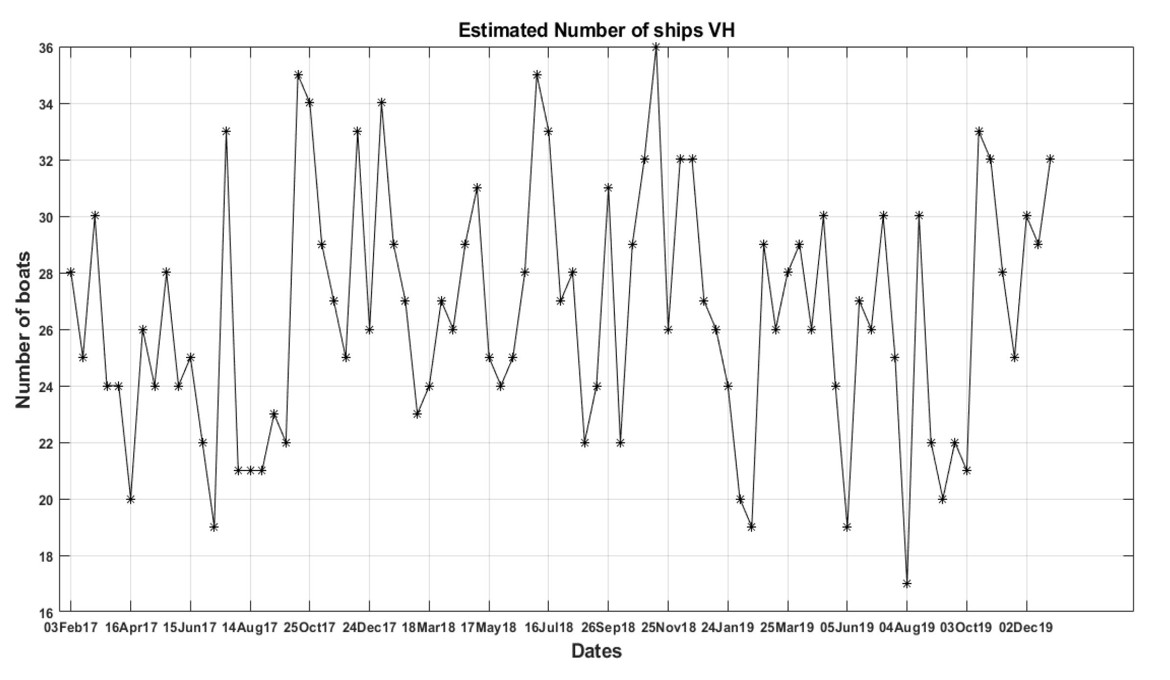
5.2.3. Ship Number Estimation within the Scene Using the FBR Procedure

We focus now on the estimation of the number of ships for each acquisition. First, a mask was defined to exclude possible changes coming from the land areas, as shown in annex Figure A3 in light blue. It is now possible to estimate the number of ships for each acquisition by using the FBR procedure and setting a threshold on the raw output CD for each acquisition. The change detection map can be superimposed with the reference image when the user is interested in a specific date to improve the interpretation, as shown in Figure 20b,d, and can evaluate the ship traffic for a given date.

The MATLAB function bwconncomp was used to determine the number of binary objects forming a group of pixels detected within the scene. The estimated ship number for each acquisition date is presented in Figure 21 for VH. To verify the consistency of the results, we proposed considering the dates where we detected the lowest and the highest number of ships. For these dates, we display in Figure 20 the radiometric images and the CD maps obtained from our FBR method.

These acquisitions corresponded to the 13 November 2018 as shown in Figure 20c for the highest attendance of 36 ships and 4 August 2019 for the lowest attendance in Figure 20a with 17 ships. As we can observe from the radiometric images visually, most of the quays were free of ships, and few ships were visible on the open sea for the acquisition of 4 August 2019. On the contrary, for the 13 November 2018, the number of ships moored to the quays and in the open sea appears to be significantly higher. The number of ships detected from the method was accurate according to the chosen radiometric images. However, it was not possible to verify on each image the number of boas with only SAR images. It would be interesting to evaluate the procedure on a dataset with ground truth (optical images for example) to characterize the method fully.

6. Discussion

The different results presented in this article demonstrated the advantages of the proposed method. We aimed to understand the impact of target SNR and the number of dates on the detection capability of such a framework. The method enabled comparable detection capabilities when the target SNR was sufficiently high (over 6 dB) and has an advantage to produce better results when the target SNR was below 6 dB.

In terms of interpretation, the FBR method was more suitable and consistent with reality as the change was not performed relatively between two dates but from an estimated stable scene. This was one significant advantage compared to the methods of multi-temporal CD in SAR images proposed in the literature. As shown through the different results, the FBR procedure was interesting when the purpose was to determine the number of ephemeral objects at a specific date. However, the computation of the FBR image can become a difficult task with a background subject to temporal periodical variation (agriculture conditions), or with an important background change (demolition of a quarter). These configurations have to be taken into account to improve the proposed method and implement it in a wider range of applications.

Further studies must be performed to understand the sensitivity of the FBR images with the SAR system parameters. For the specific case of the studied area, we could reach the stability of the computed FBR image after 30 dates with a temporal resolution of 2 weeks. This represents around a year of Sentinel 1 acquisitions. The proposed framework was also designed to consider future satellite missions that can offer a much higher temporal resolution.

In addition, this study was conducted only in a monopolarisation case. Additional studies must be performed on the polarimetric behavior of an FBR scene. The stability of a scene, and thus the number of dates required to achieve a good background estimation, might be highly dependent on the operating frequency of the sensor as well as the resolution due to the intrinsic physical phenomenons of the scene.

7. Conclusions

In this article, the concept of frozen background reference image based change detection was introduced for target detection. The simulations showed that the interpretation was improved as well as the detection capabilities for targets mixed with Gaussian noise in a SAR time-series. The use of several acquisitions improved the detection capabilities in the case of a low target SNR. An application on industrial harbor traffic monitoring was proposed using this method. In the future, testing on a dataset with known ground truth is needed to evaluate the performances of detection and extend it to a larger scale of applications. This concept can be applied in several configurations for target detection. The Sentinel data resolution here was suitable to detect ships. However, it would be interesting to test this method with a higher resolution in dense urban areas. The FBR image played a crucial role in making sure that the scene was empty and excluding possible misinterpretations. As shown in this article, this method enabled us to more easily interpret the CD map.

References

1. El-Darymli, K.; McGuire, P.; Power, D.; Moloney, C. Target detection in Synthetic Aperture Radar imagery: A State-of-the-Art Survey. J. Appl. Remote Sens. 2013, 7, 071598. [Google Scholar] [CrossRef] [Green Version]
2. Novak, L.M. Change detection for multi-polarization multi-pass SAR. Proc. SPIE 2005, 5808, 234–246. [Google Scholar] [CrossRef]
3. Conradsen, K.; Nielsen, A.A.; Schou, J.; Skriver, H. A test statistic in the complex Wishart distribution and its application to change detection in polarimetric SAR data. IEEE Trans. Geosci. Remote Sens. 2003, 41, 4–19. [Google Scholar] [CrossRef] [Green Version]
4. Koeniguer, E.C.; Nicolas, J.M. Change Detection in SAR Time-Series Based on the Coefficient of Variation. Available online: https://arxiv.org/pdf/1904.11335.pdf (accessed on 20 April 2020).
5. Davidson, M.; Chini, M.; Dierking, W.; Djavidnia, S.; Djavidnia, S.; Haarpaintner, J.; Hajduch, G.; Laurin, G.V.; Lavalle, M.; Martinez, C.L.; et al. Copernicus L-Band SAR Mission Requirements Document; Technical Report; European Space Agency (ESA-ESTEC, Netherlands): Noordwijk, The Netherlands, 2018; Available online: https://esamultimedia.esa.int/docs/EarthObservation/Copernicus_L-band_SAR_mission_ROSE-L_MRD_v2.0_issued.pdf (accessed on 25 April 2020).
6. Torres, R.; Lokas, S.; Moller, H.L.; Zink, M.; Simpson, D.M. The TerraSAR-L mission and system. In Proceedings of the 2004 IEEE International Geoscience and Remote Sensing Symposium, Anchorage, AK, USA, 20–24 September 2004; Volume 7, pp. 4519–4522. [Google Scholar]
7. Carotenuto, V.; De Maio, A.; Clemente, C.; Soraghan, J. Unstructured Versus Structured GLRT for Multipolarization SAR Change Detection. IEEE Geosci. Remote Sens. Lett. 2015, 12, 1665–1669. [Google Scholar] [CrossRef] [Green Version]
8. Anfinsen, S.N.; Doulgeris, A.P.; Eltoft, T. Estimation of the Equivalent Number of Looks in Polarimetric Synthetic Aperture Radar Imagery. IEEE Trans. Geosci. Remote Sens. 2009, 47, 3795–3809. [Google Scholar] [CrossRef]
9. Sentinel Application Platform (SNAP). Version 7.0.0. Available online: http://step.esa.int/main/toolboxes/snap/ (accessed on 20 April 2020).
Figure 1. Multi bi-date change detection.
Remotesensing 12 01720 g001
Figure 2. Frozen background reference (FBR) based change detection (CD) using Synthetic Aperture Radar (SAR) time-series.
Remotesensing 12 01720 g002
Figure 3. Candidate pixel selection within the time-series.
Remotesensing 12 01720 g003
Figure 4. Inhomogenous dimensions in time direction of candidate pixels.
Remotesensing 12 01720 g004
Figure 5. Simulated scenes and associated reference images.
Remotesensing 12 01720 g005
Figure 6. Histogram of radiometric scene, MP and RP FBR images.
Remotesensing 12 01720 g006
Figure 7. Example of the CD ground truth and change map for SNR = 3 dB.
Remotesensing 12 01720 g007
Figure 8. ROC curves for different target SNRs.
Remotesensing 12 01720 g008
Figure 9. ROC (Receiver Operating Characteristic) curves representing PD (probality of detection) and PFA (probabiblity of false alarm) for different amounts of images used to create the FBR scene.
Remotesensing 12 01720 g009
Figure 10. ROC (Receiver Operating Characteristic) curves for polarimetric vectors.
Remotesensing 12 01720 g010
Figure 11. Example of floating platforms over this lake, seen on Google Earth images.
Remotesensing 12 01720 g011
Figure 12. Radiometric UAVSAR image and MP and RP reference images.
Remotesensing 12 01720 g012
Figure 13. CD results for RP and MP modes.
Remotesensing 12 01720 g013
Figure 14. FBR image Projected on Google Maps (study area within the red rectangle).
Remotesensing 12 01720 g014
Figure 15. FBR image and area of interest: (a) Google Maps image, (b) Google Maps image and FBR image with 50% transparency, (c) FBR image projected on the Google Maps image.
Remotesensing 12 01720 g015
Figure 16. Mean error ϵ ¯ depending on the number of images used to compute the FBR image.
Remotesensing 12 01720 g016
Figure 17. Consecutive radiometric images for VH polarisation: (a) Radiometric VH 13 October 2017, (b) Radiometric VH 25 October 2017 (Sentinel 1 GRD data).
Remotesensing 12 01720 g017
Figure 18. Raw output CD comparison for the dates 13/10/2017 and 25/10/2017: (a) Classical Bidate VH, (b) Classical Bidate VV, (c) CD FBR for date 13/10/2017 VH, (d) CD FBR for date 13/10/2017 VV, (e) CD FBR for date 25/10/2017 VH, (f) CD FBR for date 25/10/2017 VH.
Remotesensing 12 01720 g018
Figure 19. (a) Four dates Omnibus change detection analysis, (b) CD FBR computation on the four first dates.
Remotesensing 12 01720 g019
Figure 20. Images of highest and lowest attendance detected with the FBR method: (a) Radiometric 4 August 2019, (b) CD FBR 4 August 2019, (c) Radiometric 13 November 2018 and (d) CD FBR 13 November 2018.
Remotesensing 12 01720 g020
Figure 21. Estimated number of ships per acquisition.
Remotesensing 12 01720 g021