Letter

Wishart-Based Adaptive Temporal Filtering of Polarimetric SAR Imagery

1
Formerly Jülich Research Center, 52425 Jülich, Germany
2
DTU Compute, Department of Applied Mathematics and Computer Science, Technical University of Denmark, 2800 Kongens Lyngby, Denmark
3
DTU Space, the National Space Institute, Technical University of Denmark, 2800 Kongens Lyngby, Denmark
*
Author to whom correspondence should be addressed.
Remote Sens. 2020, 12(15), 2454; https://doi.org/10.3390/rs12152454
Submission received: 28 June 2020 / Revised: 20 July 2020 / Accepted: 28 July 2020 / Published: 30 July 2020

Abstract

:
Temporal filtering for speckle reduction of polarimetric SARimages is described. The method is based on a sequential complex Wishart-based change detection algorithm which is applied to polarized SAR imagery, including the dual-polarization intensity data archived on the Google Earth Engine (GEE). Software for convenient application and analysis is presented. Results compare favorably with, and improve upon, standard spatial and temporal filters for speckle reduction.

Graphical Abstract

1. Introduction

A characteristic of SAR images, when compared to their visual/infrared counterparts, is the disconcerting “speckle” effect which sometimes makes visual interpretation very difficult. Speckle gives the appearance of random noise, but it is actually a deterministic consequence of the coherent nature of the radar signal. Although disadvantageous in some contexts, coherence effects in the received radar signal constitute the basis of SAR interferometry and its many applications. However, one is often concerned primarily with SAR intensity (as opposed to amplitude and phase) observations, for example, for target detection, image classification, or forest monitoring, where speckle is indeed a nuisance.
Many adaptive spatial filtering methods have been developed in the past, some of the most popular of which are described in [1,2,3,4,5,6,7,8]. In addition, temporal [9] and hybrid temporal [10] methods have been proposed for time series of SAR imagery. In this paper, we describe a straightforward adaptive temporal filter, which is essentially a by-product of a sequential change detection algorithm for times series of polarimetric SAR images [11,12,13]. In order to determine the so-called Löwner order (direction) of significant changes in the algorithm, it is necessary to keep a running average image whose pixels are updated whenever a change occurs. At the conclusion of this process, the running average is the temporally filtered version of the last image in the series. Pixels which have not changed, or which change only early in the sequence, are well averaged and exhibit little speckle. Those which change later will be less well despeckled. Since there is no convolution involved with a spatial kernel, there is no degradation of spatial resolution whatsoever. We refer to this procedure in the following as an adaptive temporal spatial filter (ATSF) and the despeckled result as the ATSF image. The method is especially useful if one is also performing a change detection study over many time points, in which case, the despeckling is a (free) by-product. The filter is unique, resolution preserving, and may be of interest for purposes other than simple visualization (speckle reduction), such as preprocessing for feature detection or for classification and segmentation by means of machine learning methods, which are insensitive to the equivalent number of looks (ENL), e.g., convolutional neural networks.

2. Theory

Complex Wishart-based change detection algorithms for bitemporal and multitemporal SAR images have been described in a series of publications [14,15,16,17,18], and applications to long time series of Sentinel-1 imagery archived on the Google Earth Engine (GEE) [19] are given in [13]. To briefly summarize the methodology, given a sequence of k SAR images in polarimetric matrix form, all characterized by the same ENL, the statistical null hypothesis Σ 1 = Σ 2 = = Σ k , where Σ j is the covariance matrix characterizing the complex Wishart probability distribution of an observed pixel in the jth image, is tested against all alternatives. This is referred to as the Q test in the cited papers. If this test is accepted, we are done: for this pixel there is no change over the time span t 1 to t k . If the test is rejected, the hypotheses
Σ 1 = Σ 2 against Σ 1 Σ 2 Σ 1 = Σ 2 = Σ 3 against Σ 1 = Σ 2 Σ 3 Σ 1 = Σ 2 = = Σ k 1 = Σ k against Σ 1 = Σ 2 = = Σ k 1 Σ k
are tested (called the R j tests [15]). In the event of rejection of the null hypothesis at any time point (significant change), the tests are restarted from that point for the image pixel concerned. See [15] for details. Subsequently, a direction measure for the observed significant changes is determined as follows: The covariance matrix prior to change is averaged over all preceding no-change images in the sequence and subtracted from the covariance matrix immediately after significant change. The Löwner order, i.e., the positive-, negative-, or in-definiteness of the difference matrix is then taken to be a measure of direction [11]. The running average image needed for the Löwner order constitutes an adaptive temporal filter on the last image in the sequence. Pixels which do not exhibit change over the full sequence are maximally averaged, and changed pixels are averaged over the period following the most recent change. In order to reduce the speckle for regions of very recent change, all averages for which the number of contributing pixels is below a threshold may be replaced by the output of an adaptive spatial filter applied to the original image. In our work, we chose the refined Lee spatial filter with 7 × 7 directional kernel [2,20], but any appropriate spatial filter can be used. It should be remarked that the only other free parameter involved in determining the ATSF is the (common) significance level chosen for the Q and R j tests. Of course, as the algorithm involves statistical testing, false negatives may result in changes being overlooked, depending on the significance level chosen.

3. Materials and Methods

Software for the sequential SAR change detection algorithm and for the adaptive temporal filter described in the preceding section is provided in Matlab (https://people.compute.dtu.dk/~{}alan/software.html) and in a Python implementation (https://github.com/mortcanty/EESARDocker) written specifically against the GEE API. The latter runs in a Docker container serving Jupyter notebooks to the user’s local browser, also see [13,20]. The precompiled Docker container can be pulled and run directly from Docker Hub and is platform independent. The filtered image is exported to the user’s Google Drive. Postprocessing Python routines for thresholding/substitution with the Lee or Gamma MAP filters are included in the container. Alternatively, refined Lee filter thresholding/substitution can be run directly within the GEE application. Long time series of archived Sentinel-1 images suitable for adaptive filtering are easily generated with the GEE, but time series from other platforms, such as RADARSAT-2, TerraSAR-X, etc., can be uploaded to the GEE platform and processed in the same way.

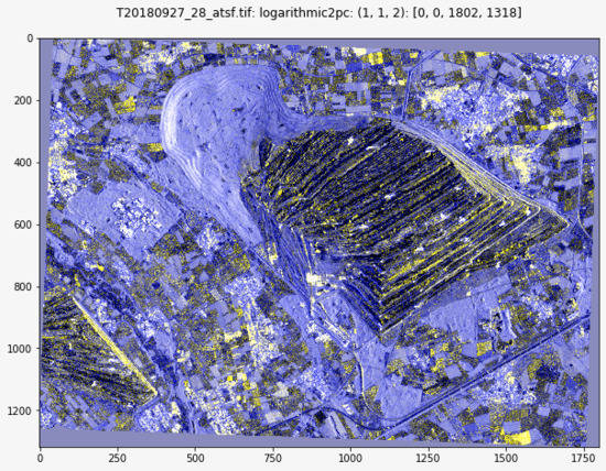
4. Results and Discussion

A Sentinel-1 image of an open-cast coal mine in Germany from 27 September 2018 is shown in Figure 1, together with the ATSF. A time series of 29 acquisitions terminating with the 27 September image was analyzed with the sequential omnibus algorithm, generating the ATSF as a side effect. As can be seen, the speckle is virtually absent from the filtered image, and land-cover boundaries and features are more easily discerned.
In Figure 2, the ATSF is compared with refined Lee [2], Gamma MAP [3], and Frost [4] spatial adaptive filters, as well as with the empirical mode decomposition (EMD) temporal filter [9] and an average over the full time series. The time average is essentially the Quegan filter [21] for uncorrelated images with the same numbers of looks and equal means.
The three spatially filtered images were produced with the Sentinel 1 Toolbox using default parameters. The EMD filtered image was calculated using the full 29-image time series in decibel (log) scale augmented with five additional images following the target date. The additional images were included in order to avoid edge effects in the empirical mode decomposition, as suggested in [9]. The Python bindings to the C-package libeemd [22] were used to program the method.
Only the Quegan filter is comparable in visual quality to the ATSF image, but being a simple time average, the earth moving machines at their locations on 27 September are no longer visible. This is also the case for the EMD filter, which otherwise has a good visual appearance. In this sense, the ATSF is, like the spatial filters but unlike the Quegan and EMD temporal filters, a despeckled version of the September 27 target image.
Figure 3 shows a subset of the reference image from 27 September with the Jülich Research Center and environs. The center itself and the forest surrounding it exhibit very little speckle after filtering (top right). However, speckle is still present in some of the nearby agricultural fields due to recent changes (harvesting). These areas also appear darker because of the lower radar cross-section in the harvested fields. The bottom left figure shows, per-pixel, the number of images used in forming the ATSF as a gray scale image, from black = 1 through to white = 29. The thresholded ATSF image (see Section 2) is shown bottom right for a threshold of 7. The speckle in the recently changed, harvested agricultural fields is now reduced by the Lee adaptive filter.
Figure 4 shows on the right, the ATSF result for a time series of 12 quad-pol RADARSAT-2 images from 2009 and 2010 over an agricultural/mixed forest area near Bonn, Germany. The ENL of the images in the series was 12, so that speckle is in any case reduced in the original image (left). However, the ATSF still improves the visual impression considerably.
Another example of the application of the ATSF filter is given in Figure 5. With its large scale structures (roads, runways, etc.), the image sequence will be used below to illustrate edge preservation/enhancement.
Evaluating and comparing speckle filters is particularly difficult because, apart from in simulations, there is no reference other than the original unfiltered image itself. Table 1 compares the mean bias criterion ( M B ) as a fidelity measure comparing various filtered images with the original image as suggested in [10], namely
M B = log μ 1 μ 2 μ 1 ,
where μ 1 and μ 2 are the mean intensities of the original and filtered images, respectively. Four adaptive spatial filters were applied using the ESA Sentinel-1 Toolbox with default parameters along with the EMD and Quegan filters. Larger values indicate better agreement with the original image. The Gamma MAP and Frost filters perform best with this metric on the chosen datasets, but the ATSF achieves acceptable results compared to the spatial filters (the EMD filter was not applied to the RadarSat-2 imagery due to the relatively short length of the time series).
The M B metric is marginal, that is, bands are compared separately. On the other hand, the average difference in spectral angle ( A D S A ) (see, e.g., [23]) allows for the comparison of the complete polarimetric images:
A D S A = arccos x 1 · x 2 | x 1 | | x 2 | ,
where x 1 and x 2 are observation vectors for the original and filtered images. Typical values are shown in Table 2. Here, the adaptive spatial filters slightly outperform the ATSF and EMD filters.
Not surprisingly, the ATSF outperforms the adaptive spatial filters at edge preservation and enhancement, since there is no spatial averaging taking place whatsoever. This can be seen clearly in Figure 6 where the Canny edge detector is applied to several spatial filters, to the EMD filter, and to the ATSF of the Frankfurt airport image in Figure 5. The EMD filter also performs better than the spatial filters but not as well as the ATSF.
Another means to compare speckle filters is on the basis of the ENL characterizing an image. The ENL describes the degree of averaging applied to the SAR measurements during data formation and postprocessing. The ENL of a speckle filter result is essentially the number of independent looks which would be needed to obtain the same degree of smoothing as that achieved by the filter itself, so that the range of ENL values within an image is an indirect measure of speckle reduction. Figure 7 shows histograms of the ENL values. These were estimated with a multivariate method described in [24]. A robust ENL estimate is extracted from the distribution of small sample estimates collected over the whole scene. Histograms of these small sample estimates collected within a 7 × 7 window passed over the scene are shown in the figure, in this case, for a heavily forested area in Germany exhibiting well-developed speckle. The upper-left histogram is for the target image without filtering and has a mode at about five equivalent looks, corresponding to the 5 × 1 (range × azimuth) multilooking carried out in the original processing. The upper-right hand histogram is for the ATSF using a time series of 29 images ending with the target image. It approximately compares to the refined Lee spatial filter with a 5 × 5 kernel (lower left).
Finally, the ratio of the original image intensities to those of the filtered image should ideally, because of the multiplicative noise assumption, be featureless noise [9]. This is largely the case for the refined Lee and Gamma MAP spatial filters (Figure 8). The ratios for the EMD and ATSF temporal filters show some land-use features. Note that the earth moving machines are absent in the ATSF ratio image, as they should be. A summarized comparison of the various speckle filters examined is given in Table 3.

5. Conclusions

The adaptive temporal speckle filter (ATSF) described here is a side effect of time series analysis with the sequential omnibus algorithm and is seen to be comparable to a conventional spatial filter with respect to the amount of smoothing achieved and fidelity to the original image, while at the same time exhibiting a much better performance at edge preservation and enhancement. It presupposes a sufficiently long and contiguous time series (in the order of 10 or more images) preceding the acquisition date of the target image, as well as a predominance of unchanged pixels over the series. The Python software described in Section 3 exploits the huge Sentinel-1 archive on the GEE to make the filter application simple and fast. The effect of recent changes in the time series can be mitigated by using a spatial filter for the corresponding pixels. In the worst case of predominating recent changes, the ATSF (in our software implementation) reduces to the refined Lee spatial filter.

Author Contributions

Conceptualization, M.J.C. and A.A.N.; Formal analysis, K.C. and A.A.N.; Funding acquisition, A.N.; Methodology, A.A.N., H.S. and K.C.; Software, M.J.C.; Supervision, A.N. and H.S.; Visualization, M.J.C.; Writing—original draft, M.J.C.; Writing—review & editing, M.J.C., A.A.N., H.S. and K.C. All authors have read and agreed to the published version of the manuscript.

Funding

This research received no external funding.

Conflicts of Interest

The authors declare no conflict of interest.

References

  1. Lee, J.S. Digital enhancement of noise filtering by use of local statistics. IEEE Trans. Pattern Anal. Mach. Intell. 1980, 165–168. [Google Scholar] [CrossRef] [Green Version]
  2. Lee, J.S.; Grunes, M.R.; de Grandi, G. Polarimetric SAR speckle filtering and its implication for classification. IEEE Trans. Geosci. Remote Sens. 1999, 37, 2363–2373. [Google Scholar]
  3. Oliver, C.; Quegan, S. Understanding Sythetic Aperture Radar Images; SciTech: West Perth, Australia, 2004. [Google Scholar]
  4. Frost, V.S.; Stiles, J.A.; Shanmugan, K.S.; Holtman, J.C. A model for radar images and its application to adaptive digital filtering of multiplicative noise. IEEE Trans. Pattern Anal. Mach. Intell. 1982, 4, 157–166. [Google Scholar] [CrossRef] [PubMed]
  5. Vasile, G.; Trouvé, E.; Lee, J.S.; Buzuloiu, V. Intensity-Driven-Adaptive-Neighborhood Technique for Polarimetric and Interferometric SAR Parameters Estimation. IEEE Trans. Geosci. Remote Sens. 2006, 44, 1609–1621. [Google Scholar] [CrossRef] [Green Version]
  6. Kuan, D.T.; Sawchuk, A.A.; Strand, T.C.; Chavel, P. Adaptive Noise Smoothing Filter for Images with Signal-Dependent Noise. IEEE Trans. Pattern Anal. Mach. Intell. 2009, 165–177. [Google Scholar] [CrossRef] [PubMed]
  7. Deledalle, C.A.; Denis, L.; Poggi, G.; Tupin, F.; Verdoliva, L. Exploiting patch similarity for SAR image processing: The nonlocal paradigm. IEEE Signal Process. Mag. 2014, 31, 69–78. [Google Scholar] [CrossRef]
  8. Deledalle, C.; Denis, L.; Tupin, F.; Reigber, A.; Jäger, M. NL-SAR: A Unified Nonlocal Framework for Resolution-Preserving (Pol)(In)SAR Denoising. IEEE Trans. Geosci. Remote Sens. 2015, 53, 2021–2038. [Google Scholar] [CrossRef] [Green Version]
  9. Cremer, F.; Urbazaev, M.; Berger, C.; Mahecha, M.D.; Schmullius, C.; Thiel, C. An Image Transform Based on Temporal Decomposition. IEEE Geosci. Remote Sens. Lett. 2018, 15, 537–541. [Google Scholar] [CrossRef] [Green Version]
  10. Yuan, J.; Lv, X.; Li, R. A Speckle Filtering Method Based on Hypothesis Testing for Time-Series SAR Images. Remote Sens. 2018, 10, 1383. [Google Scholar] [CrossRef] [Green Version]
  11. Nielsen, A.A.; Skriver, H.; Conradsen, K. The Loewner Order and Direction of Detected Change in Sentinel-1 and Radarsat-2 Data. IEEE Geosci. Remote Sens. Lett. (Early Access June 2019) 2020, 17, 242–246. [Google Scholar] [CrossRef] [Green Version]
  12. Nielsen, A.A. Fast matrix based computation of eigenvalues and the Loewner order in PolSAR data. IEEE Geosci. Remote Sens. Lett. (Early Access) 2019, 1–5. [Google Scholar] [CrossRef]
  13. Canty, M.J.; Nielsen, A.A.; Skriver, H.; Conradsen, K. Statistical Analysis of Changes in Sentinel-1 Time Series on the Google Earth Engine. Remote Sens. 2019, 12, 46. [Google Scholar] [CrossRef] [Green Version]
  14. Conradsen, K.; Nielsen, A.A.; Schou, J.; Skriver, H. A test statistic in the complex Wishart distribution and its application to change detection in polarimetric SAR data. IEEE Trans. Geosci. Remote Sens. 2003, 41, 4–19. [Google Scholar] [CrossRef] [Green Version]
  15. Conradsen, K.; Nielsen, A.A.; Skriver, H. Determining the points of change in time series of polarimetric SAR data. IEEE Trans. Geosci. Remote Sens. 2016, 54, 3007–3024. [Google Scholar] [CrossRef] [Green Version]
  16. Nielsen, A.A.; Conradsen, K.; Skriver, H.; Canty, M.J. Visualization of and software for omnibus test based change detected in a time series of polarimetric SAR data. Can. J. Remote Sens. 2017, 43, 582–592. [Google Scholar] [CrossRef]
  17. Conradsen, K.; Nielsen, A.A.; Skriver, H. Omnibus change detection in block diagonal covariance matrix PolSAR data from Sentinel-1 and Radarsat-2. In preparation.
  18. Akbari, V.; Anfinsen, S.N.; Doulgeris, A.P.; Eltoft, T.; Moser, G.; Serpico, S.B. Polarimetric SAR change detection with the complex Hotelling-Lawley trace statistic. IEEE Trans. Geosci. Remote Sens. 2016, 54, 3953–3966. [Google Scholar] [CrossRef] [Green Version]
  19. Gorelick, N.; Hancher, M.; Dixon, M.; Ilyushchenko, S.; Tau, D.; Moore, R. Google Earth Engine: Planetary-scale geospatial analysis for everyone. Remote Sens. Environ. 2017, 202, 18–27. [Google Scholar] [CrossRef]
  20. Canty, M.J. Image Analysis, Classification, and Change Detection in Remote Sensing, With Algorithms for ENVI/IDL and Python, 4th ed.; Taylor and Francis: Boca Raton, FL, USA, 2019. [Google Scholar]
  21. Quegan, S.; Yu, J.J. Filtering of multichannel SAR images. IEEE Trans. Geosci. Remote Sens. 2001, 39, 2373–2379. [Google Scholar] [CrossRef]
  22. Luukko, P.; Helske, J.; Räsänen, E. Introducing libeemd: A program package for performing the ensemble empirical mode decomposition. Comput. Stat. 2015, 31, 545–557. [Google Scholar] [CrossRef] [Green Version]
  23. Yuhas, R.; Goetz, A.; Boardman, J. Discrimination among semi-arid landscape endmembers using the Spectral Angle Mapper (SAM) algorithm. In JPL, Summaries of the Third Annual JPL Airborne Geoscience Workshop. Volume 1: AVIRIS Workshop; NASA: Washington, DC, USA, 1992; pp. 147–149. [Google Scholar]
  24. Anfinsen, S.; Doulgeris, A.; Eltoft, T. Estimation of the equivalent number of looks in polarimetric synthetic aperture radar imagery. IEEE Trans. Geosci. Remote Sens. 2009, 47, 3795–3809. [Google Scholar] [CrossRef]
Figure 1. Top: RGB composite ( R = | S v v | 2 , G = | S v v | 2 , B = | S v h | 2 ) of a polarimetric Sentinel-1 SAR image acquired 27 Sept 2018 over the Hambach open-cast mine near Jülich, Germany. The bright features in the mine pit are very large mobile excavators and back fillers. Bottom: The adaptive temporal speckle filter (ATSF).
Remotesensing 12 02454 g001
Figure 2. Comparison of six spatial and temporal speckle filters: Refined Lee (top left), Gamma MAP (top right), Frost (center left), empirical mode decomposition (EMD) (center right), Quegan (bottom left), and ATSF (bottom right) for a spatial subset of the reference image, | S v v | 2 band only. Note that the earth moving machines are absent in both the Quegan and EMD filters.
Remotesensing 12 02454 g002
Figure 3. Comparison of the original image (top left) and ATSF (top right) for a small spatial subset of the reference image of Figure 1. Bottom left: the number of images used in forming the ATSF, black = 1, white = 29. Bottom right: the thresholded ATSF.
Remotesensing 12 02454 g003
Figure 4. Comparison of a RADARSAT-2 quad-polarized image acquired over an area southwest of Bonn, Germany on 11 Oct 2010 (left) with the ATSF derived from a sequence of 12 images from 25 May 2009 through to 11 Oct 2010 (right). The images are in the Pauli representation ( R = | S h h S v v | 2 , G = | S h v | 2 , B = | S h h + S v v | 2 ). RADARSAT-2 Data and Products ©MacDonald, Dettwiler and Associates Ltd. (2009–2010) — All Rights Reserved. RADARSAT is an official trademark of the Canadian Space Agency.
Remotesensing 12 02454 g004
Figure 5. The Frankfurt International Airport. Left: A Sentinel-1 scene acquired on 27 October 2018 taken from the Google Earth Engine (GEE) archive. Right: The result of applying the ATSF to a series of 33 images beginning 6 April and ending with the 27 October image.
Remotesensing 12 02454 g005
Figure 6. Illustrating edge preservation. From left to right, top to bottom: a spacial subset of the airport image for 27 October; canny edges for the refined Lee filter; for the Gamma MAP filter; for the Frost filter; for the EMD filter; and for the ATSF.
Remotesensing 12 02454 g006
Figure 7. Histograms of the equivalent number of looks (ENL) for a Sentinel-1 scene over a wooded area in Germany; (upper left): for the target image acquired 26 September 2018; (upper right): for the ATSF using a time series of 29 images beginning 5 April and ending 26 September 2018; (lower left): for the refined Lee filter of the target image with a 5 × 5 kernel; (lower right): for the the refined Lee filter with a 7 × 7 kernel.
Remotesensing 12 02454 g007
Figure 8. RGB composite ratios ( R = G = | S v v | 2 / | S ^ v v | 2 , B = | S v h | 2 / | S ^ v h | 2 ) of the target image to the refined Lee filter (upper left), the Gamma MAP filter (upper right), the EMD filter (lower left), and the ATSF (lower right) for the same spatial subset as Figure 2.
Remotesensing 12 02454 g008
Table 1. Comparison of mean bias values, best results in boldface.
Scene (Platform)BandLee [2]Gamma [3]Frost [4]IDAN [5]EMD [9]Quegan [21]ATSF
Hambach (S1) | S v v | 2 2.523.494.522.121.53−0.043.33
| S v h | 2 2.773.274.552.251.520.003.06
Bonn (RS2) | S h h | 2 3.044.404.341.86 2.882.77
| S h v | 2 2.304.733.601.12 2.332.58
| S v v | 2 3.144.314.651.90 2.042.21
Frankfurt (S1) | S v v | 2 1.422.703.010.912.47−0.072.64
| S v h | 2 1.792.953.411.343.41−0.02.02
Table 2. Comparison of mean spectral angle differences in degrees, best results in boldface.
Scene (Platform)Lee [2]Gamma [3]Frost [4]IDAN [5]EMD [9]Quegan [21]ATSF
Hambach (S1)2.802.252.573.976.31129.84.44
Bonn (RS2)5.263.615.987.86 10.3810.13
Frankfurt (S1)3.232.853.104.858.01134.37.27
Table 3. Qualitative comparison of despeckling methods.
FilterFidelity 1 ResolutionRemarks
Spatial 2 GoodModerate
QueganPoorGoodRecent details averaged away
EMDModerateGoodRecent details averaged away
ATSFModerateGoodRequires time series
1 MB, ADSA, ratio; 2 Lee, Gamma, Frost, IDAN.

